An Integrated Building Energy Model in MATLAB

Abstract

This paper discusses the development of an Integrated Building Energy Model (IBEM) in MATLAB (R2024b) for a university campus building. In the general context of the development of integrated energy district models to guide the evolution and planning of smart energy grids for increased efficiency, resilience, and sustainability, this work describes in detail the development and use of an IBEM for a university campus building featuring a heat pump-based heating/cooling system and PV generation. The IBEM seamlessly integrates thermal and electrical aspects into a complete physical description of the energy performance of a smart building, thus distinguishing itself from co-simulation approaches in which different specialized tools are applied to the two aspects and connected at the level of data exchange. Also, the model, thanks to its physical, white-box nature, can be instanced repeatedly within the comprehensive electrical micro-grid model in which it belongs, with a straightforward change of case-specific parameter settings. The model incorporates a heat pump-based heating/cooling system and photovoltaic generation. The model’s components, including load modeling, heating/cooling system simulation, and heat pump implementation are described in detail. Simulation results illustrate the building’s detailed power consumption and thermal behavior throughout a sample year. Since the building model (along with the whole campus micro-grid model) is implemented in the MATLAB Simulink environment, it is fully portable and exploitable within a large, world-wide user community, including researchers, utility companies, and educational institutions. This aspect is particularly relevant considering that most studies in the literature employ co-simulation environments involving multiple simulation software, which increases the framework’s complexity and presents challenges in models’ synchronization and validation.

1. Introduction

The integration of buildings as active components of smart electric grids—particularly in the micro-grid context—is a process in rapid acceleration for environmental as well as economic reasons [1,2,3]. The penetration of Distributed Energy Resources (DERs)—in this context, chiefly photovoltaic (PV) power generation—coupled with Battery Energy Storage Systems (BESSs), and the electrification of heating via heat pumps, are rapidly changing the role of buildings from pure and relatively simple electric loads into more complicated entities with the possibility of energy self-sufficiency (at least for limited stretches of time) and active contributions to grid management with injections of excess power production and sharing of energy storage capabilities [2,3,4,5,6]. In the evolution of urban environments along the Smart City path, smart energy grids and micro-grids (MGs) are and increasingly will be essential components, and buildings will be key players in the process [7,8].

The growing complexity of the energy identity and role of buildings calls for a new level of attention to the modeling of their energy footprints, both passive (consumption) and active (generation) [9,10]. Historically, building models have evolved in the direction of increasing environmental and sustainability awareness (from the Intelligent Building to the Smart Building, to the Green Building, and finally to the Zero Energy Building), as well as in that of enhanced inward and outward functionalities and services (the Grid-interactive Efficient Building) [11].

On top of that, the trend toward complete electrification of building heating/cooling systems requires that electrical and thermal energy models are integrated in a unified comprehensive approach [12], traditionally focusing each on its specific domain and using different tools and modeling approaches.

The general context in which this work belongs is that of the development of integrated energy district models to guide the evolution and planning of smart energy grids for increased efficiency, resilience, and sustainability. A remarkable example is given by [13], which takes into consideration the energy demand of a whole neighborhood, with the main objective of developing and deploying a monitoring plan to be coupled with a model for the simulation of energy performance. A detailed breakdown of the energy paths and the good match between measured and simulated data were shown. Generally speaking, district-scale and urban-scale energy models have been the subject of extensive research activity at least since the early 2000s: see for example [14] for a comprehensive review touching the aspects of climate modeling, building energy demand, energy infrastructure modeling, building thermal performance simulation, and transportation modeling. Our recent activity in particular has resulted in the creation of a complete electrical model of the University of Parma South Campus (UPSC) [15,16] to be ultimately coupled with previously developed models of the thermal energy grid [17,18].

Several papers and literature reviews have been published in the past few years on topics connected with smart building energy performance modeling and Building Energy Management System development (BEMS), a few representative examples of which are reviewed hereafter.

In [19] the focus is on building thermal simulation and optimization of Heating, Ventilation Air Conditioning System (HVAC) operation. HVAC optimization and thermal simulation—the latter carried out using a lumped element thermal model based on the equivalent electric circuit approach—are performed by two separate software tools.

The aspect of electrical energy consumption on the other hand is tackled by Moya et al. [20], as applied to a smart building with PV generation, electric energy storage, and Electric Vehicle (EV) facilities, with the goal of minimizing the energy supplied by the power grid and, consequently, the energy cost.

Other studies have considered both aspects, i.e., thermal and electrical, in their building energy models. In [21], for instance, the BEMS features two power loops, the thermal one and the electrical one, separate except in that they are both connected to a Combined Heat and Power (CHP) fuel cell, the goal being minimization of energy consumption and building automation. A co-simulation approach, i.e., the use of two independent but coupled software tools, is also presented in [22]: here the tools are the EnergyPlus^® engine for building-level energy modeling and a Modelica library for the electrical distribution system. This approach makes it possible to exploit the specific strength of each tool, thus offering accurate system modeling on both accounts, but requires taking care of tool coupling and data exchange, here leveraging the Functional Mock-up Interface (FMI) approach. Model validation was successful, albeit limited to a very simple testbed. The relevant literature on the co-simulation of buildings and smart energy systems in general is reviewed with a taxonomic approach in [23].

In this context, this work describes in detail the development and use of an Integrated Building Energy Model (IBEM) for a university campus building featuring a heat pump-based heating/cooling system, PV generation, and BESS. The IBEM combines the dynamic thermal model with the electric grid model, providing a flexible tool for analyzing and designing smart energy buildings. The main features that characterize this work with respect to the scenario outlined above are the following:

-

The model seamlessly integrates thermal and electrical aspects into a complete, physical description of the energy performance of a smart building;

-

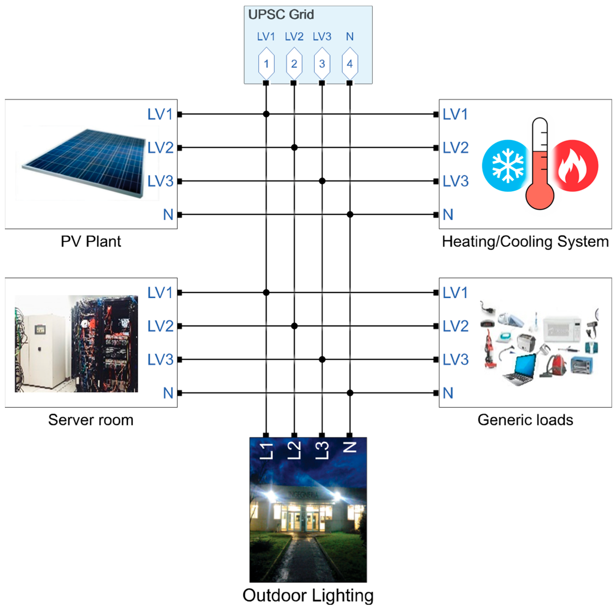
The building model is inserted into a comprehensive electrical model of a micro-grid (namely, that of the University of Parma South Campus); given its standard smart building features of grid connection, PV rooftop generation, heat pump-based conditioning system, blueprint-based thermal exchange parameters, and generic load consumption description, the model can be instanced repeatedly within the micro-grid model with case-specific parameter settings;

-

Unlike other available models based on a data-driven approach, ours is based on physical/analytical descriptions of the components, which makes it easily adaptable and scalable and provides it with predictive capabilities in the planning phase;

-

the whole model (IBEM and micro-grid) is implemented in the MATLAB Simulink environment, thus being fully portable and exploitable within the very wide community of MATLAB users, including researchers, utility companies, educational institutions (e.g., the University of Parma provides free access to MATLAB to all of its students via a Campus Agreement License); this aspect is particularly relevant considering that most studies in the literature employ co-simulation environments involving multiple simulation software, which increases the framework’s complexity [22] and presents challenges in models’ synchronization and validation [23].

The main goal of the present work is therefore the development of a MATLAB Simulink IBEM model based on a physical description of the relevant components, including PV generation, heat pump-based conditioning system, and thermal and electric loads, to be seamlessly integrated into our campus microgrid model; since it is based on an actual campus building, the IBEM can be experimentally validated and be adapted to describe new smart/green buildings thus helping the future development of the campus microgrid.

The structure of the paper is the following: Section 2 deals with the modeling approach and briefly describes the campus MG model in which the IBEM is inserted; Section 3 describes the IBEM in detail, while examples of simulation results are illustrated in Section 4; finally, Section 5 draws conclusions and outlines future developments.

2. Modeling Approach and Campus Micro-Grid Model

The UPSC MG model [15,16] was built in MATLAB Simulink using the Simscape Electrical Specialized Power Systems library to study and guide campus evolution in the direction of a smart energy district. For the sake of reducing the computational overhead of the calculation of economic and environmental sustainability figures over long periods of time, we adopted a constant-frequency discrete-time three-phase phasor-domain simulation [24]. The UPSC grid model, connected to a voltage source representing the national utility grid at the Point of Common Coupling (PCC), features a transformation cabinet at each node, transferring power from medium-voltage to low-voltage utilities, physical descriptions of the cables with per unit length values of resistance, inductance, and capacitance, and specific in-house-developed blocks modeling PV generation facilities (with Maximum Power Point Tracking), BESSs, electric vehicle charging stations, and a variety of loads including classrooms, scientific laboratories, offices, sport facilities, canteens and cafeterias; building and street outdoor lighting is also modeled. Full details and a schematic diagram of the UPSC MG can be found in [16].

3. Integrated Building Energy Model

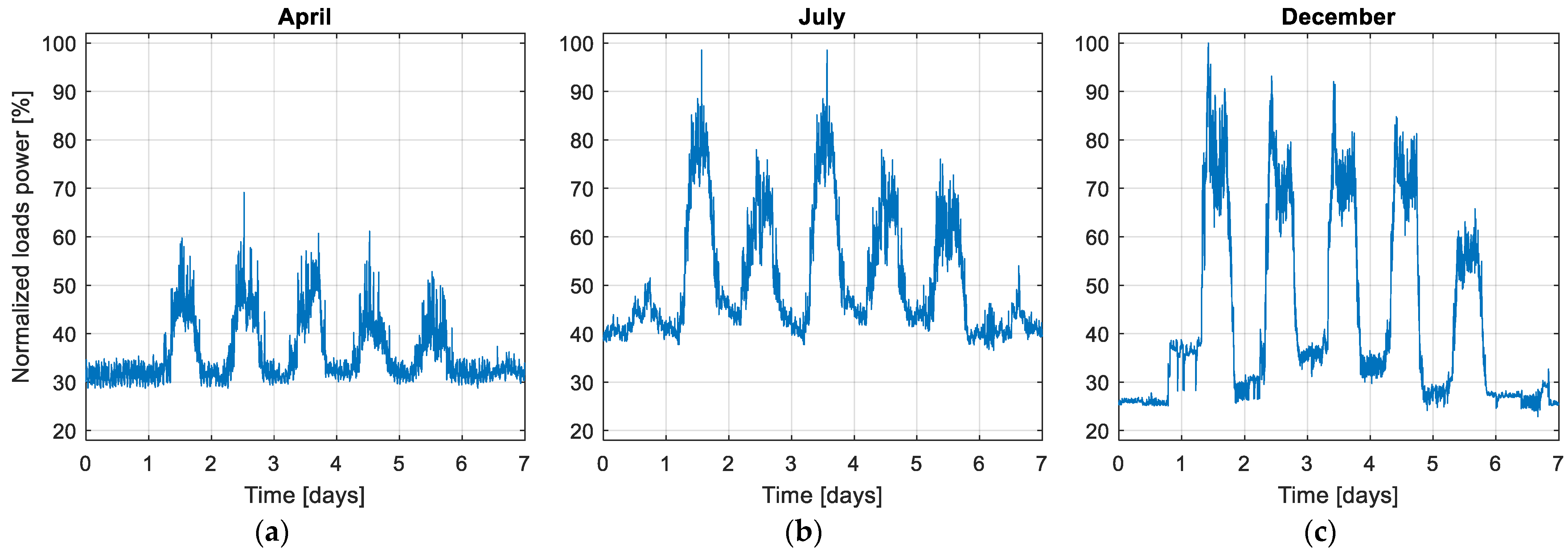
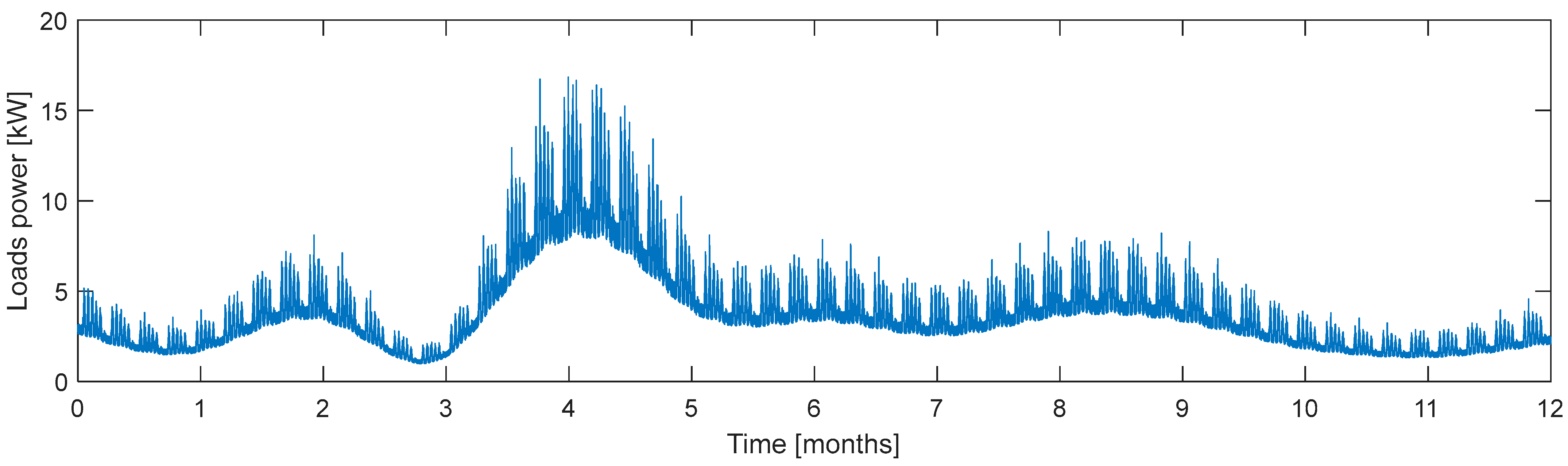
In this section we provide a detailed description of the VisLab building, which is one of the most recently built facilities in the UPSC. The building hosts a spinoff company working in the field of autonomous driving and computer vision, and features offices, laboratories (generic loads), and a server room. Unlike the other campus buildings, it is equipped with its own heat pump heating/cooling system, which makes it independent of the central campus heating/cooling system. In addition, the building features a 27 kW_p PV rooftop plant.

Figure 1 shows a schematic block diagram of the IBEM of the VisLab building, as implemented in MATLAB Simulink. The three-phase plus neutral AC lines of the campus electric grid are connected to the heat pump-based heating/cooling system, the loads (generic electric loads, the server room, and outdoor lighting), and the PV plant.

3.1. Load Modeling

Loads are modeled considering weekly power consumption profiles. Due to the limited deployment of the planned smart metering network we had to depend on data from legacy meters that record monthly consumption for selected buildings.

To address this limitation, we choose to consider typical weekly consumption profiles for offices and research laboratories obtained from measurement campaigns performed on a few selected UPSC buildings during different seasonal periods (April, July, and December) with 10 s resolution. These load profiles were then scaled based on the annual consumption trend (derived from the monthly data recorder on the VisLab building) to obtain a realistic overall load profile.

Figure 2 shows normalized weekly power profiles recorded from representative office and research laboratory facilities in the UPSC framework. These profiles are extended and integrated with monthly consumption trends to obtain the annual consumption profile illustrated in Figure 3.

Additional details about the modeling of loads and outdoor lighting power consumption can be found in [16].

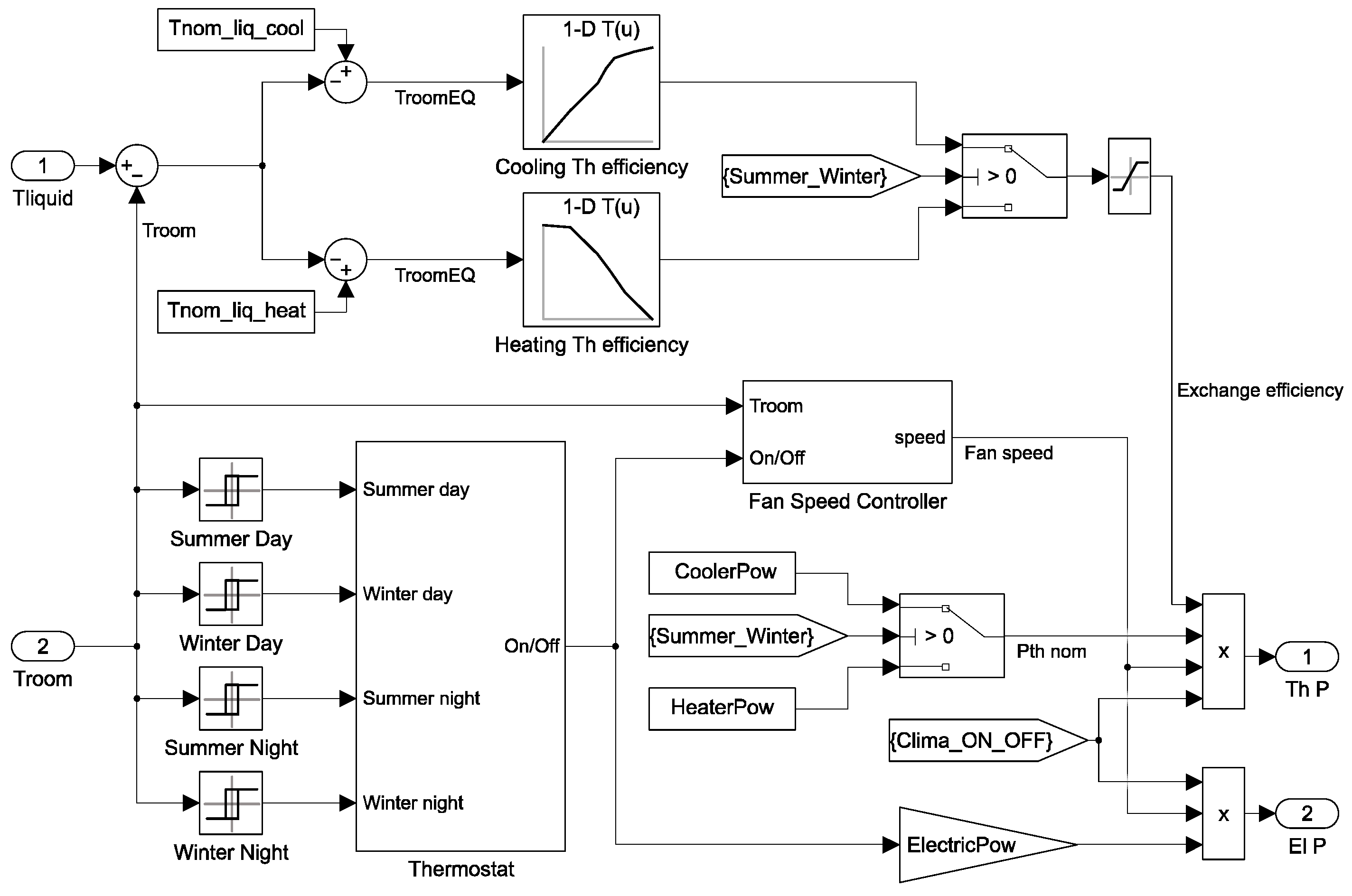
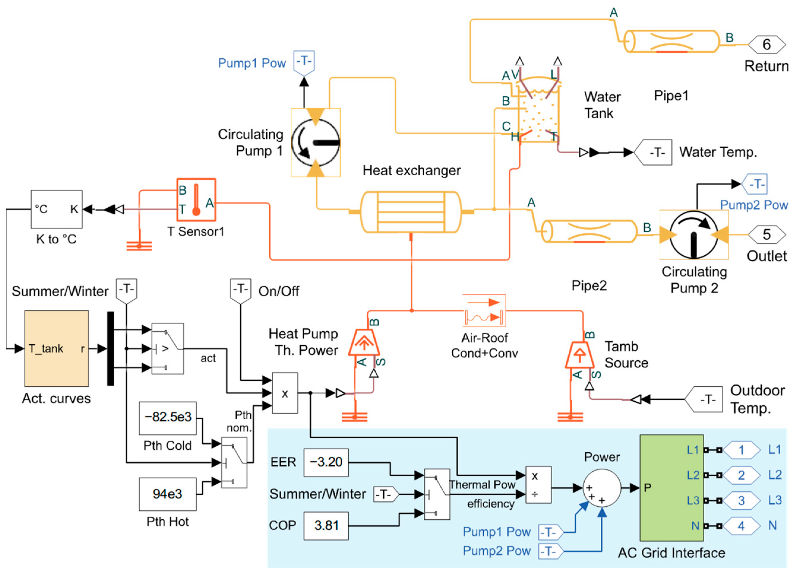
3.2. Building Heating/Cooling System Modeling

The integration of thermal and electrical energy aspects into a single model is going to receive more and more attention in the literature due to the increasing diffusion of heat pump systems, often fed by rooftop PV [25,26]. This subsection shows an example of a combined electrical/thermal model.

In order to reduce the model’s complexity, we combined all the rooms into a single building Air Thermal Mass. Similarly, the roof, walls, and windows are each represented by a single thermal mass. Figure 4 shows the Simulink implementation, where the thermal masses describing the roof, walls, and windows are connected on one side to the indoor air thermal mass and on the other side to the external atmosphere. The heat conduction and convection coefficients serve as input parameters regulating the heat flow on either side. The outdoor air temperature comes from a regional dataset of measured climate data.

The conductive and convective heat transfers are modeled by means of the library elements Conductive Heat Transfer and Convective Heat Transfer implementing, respectively, the Fourier and Newton laws in the MATLAB Simscape environment.

In

Table 1. Main parameters of the thermal network representing the building.

Parameter	Roof	Walls and Floor	Windows	Internal Volume
Heat transfer coefficient [W·m−2·K−1]	12	24	25	-
Thermal conductivity [W·m−1·K−1]	0.038	0.038	0.78	-
Area [m2]	770	800	60	-
Thickness [m]	0.2	0.2	0.01	-
Mass of the air [kg]	4925	307,200	1620	9475
Specific heat [J·K−1·kg−1]	835	835	840	1005

we summarize the main parameters of the thermal network representing the building. They are derived from the building architectural project according to the UNI Italian standards UNI 10077-1 [27] (regarding the transmittance of window components), UNI 10351 [28] (regarding the thermo-physical properties of construction materials), and UNI 10355 [29] (regarding the thermal resistance of the hollow core concrete slab area).

The heating or cooling action performed by the fan coil units is modeled by means of a controlled thermal Power Source that transfers heat from the convector coil to the indoor air mass according to the control signal Fan Coil Thermal Power. The convector coil is a pipe wherein flows the thermal fluid coming from the heat pump, with a thermal mass representing its thermal capacitance (bottom right of Figure 4).

The Fan Coil Thermal Power is computed by the Thermostat and Fan Speed Controller subsystem, the implementation of which is shown in Figure 5. The power value is obtained from the nominal heating (HeaterPow) or cooling (CoolerPow) capabilities of the fan coil, according to the season of operation—whether it is summer for cooling or winter for heating. This value is then reduced by applying two factors. The first one is the cooling/heating thermal efficiency, the second one is the normalized fan speed.

During midseasons, the fan coil stays off. However, in summer and winter, the fan is activated by a hysteresis thermostat (see Figure 5) that has the four different temperature set points shown in

Table 2. Normal and quiet modes’ temperature hysteresis thresholds applied in the Thermostat and Fan Speed Controller subsystem.

		Season
		Summer	Winter
Mode	Normal	22 ÷ 23 °C	20 ÷ 21 °C
	Quiet	26 ÷ 28 °C	13 ÷ 14 °C

, established on the basis of user comfort. These set points depend on the season and working hours. The system is designed to operate in the normal mode during working days and hours, while also offering a quiet mode. The quiet mode serves as a compromise between energy savings and the need to maintain the temperature within acceptable bounds.

When the fan coil is active, its speed depends on the difference between the room temperature and the thermostat set-point, as detailed in

Table 3. Fan speed as a function of the difference between the room temperature and the temperature set point of the thermostat controller.

ΔT = Troom − Tset	Fan Speed Level
ΔT ≤ 0.5 °C	L1 (30% of max speed)
0.5 °C < ΔT ≤ 1.5 °C	L2 (70% of max speed)
ΔT > 1.5 °C	L3 (max speed)

(in quiet mode the speed is L1).

The fan state (on/off, speed) is combined with the heat exchange efficiencies shown in Figure 6 to yield the Fan Coil Thermal Power. The equivalent room temperature on the horizontal axes of the charts in Figure 6 is not the actual room temperature but an equivalent value (Troom_EQ in Figure 5) that accounts for the variations of both room and fluid temperatures. As shown in the top left corner of Figure 5, in order to obtain the equivalent room temperature, we compute the difference between the actual liquid temperature and the reference value chosen by the fan coil manufacturer when measuring the heat exchange efficiency curves. This approach accounts for the varying behavior due to changes in liquid temperature. The computed equivalent room temperature value is finally fed as input to the efficiency curves of the fan coil, shown in Figure 6. This efficiency represents the heating/cooling capability of the fan coil based on the temperature of the environment in which it operates and is defined to be 1 at nominal room temperature, namely 20 °C in heating mode and 27 °C in cooling mode. The resulting behavior in the heating case in Figure 6 (top) shows that efficiency decreases as the actual room temperature increases and/or as the fluid temperature decreases, while the opposite happens in the cooling case.

The algorithm governing the operation of the fan coil unit model (Thermostat and Fan Speed Controller, Figure 4) is summarized by the following set of equations:

$$P_{th}=a·c_s·P_{t{h}_{nom}}·f\left(T_{roo{m}_{eq}}\right)$$

(1)

$$T_{roo{m}_{eq}}=T_{room}·\left(T_{liquid}·T_{liqui{d}_{ref}}\right)$$

(2)

$$P_{el}=b·c_s·P_{e{l}_{nom}}$$

(3)

$$a=\left\{\begin{array}{r}1, s=\mathrm{L}3\\ 0.7, s=\mathrm{L}2\\ 0.3, s=\mathrm{L}1\\ 0.05, s=\mathrm{L}0\end{array}\right.\hspace{1em}b=\left\{\begin{array}{r}1, s=\mathrm{L}3\\ 0.7, s=\mathrm{L}2\\ 0.3, s=\mathrm{L}1\\ 0, s=\mathrm{L}0\end{array}\right.$$

(4)

with

$P_{th}$	computed thermal power in watts provided by the fan coil to the indoor air mass.
$a$	fan thermal exchange capability (non-zero even when off, due to coil-to-air heat exchange).
$c_s$	binary variable indicating the activation state of the conditioning system (when zero, it means that the recirculating liquid is also stopped).
$P_{t{h}_{nom}}$	nominal thermal power in watts of a fan coil unit (different when heating or cooling).
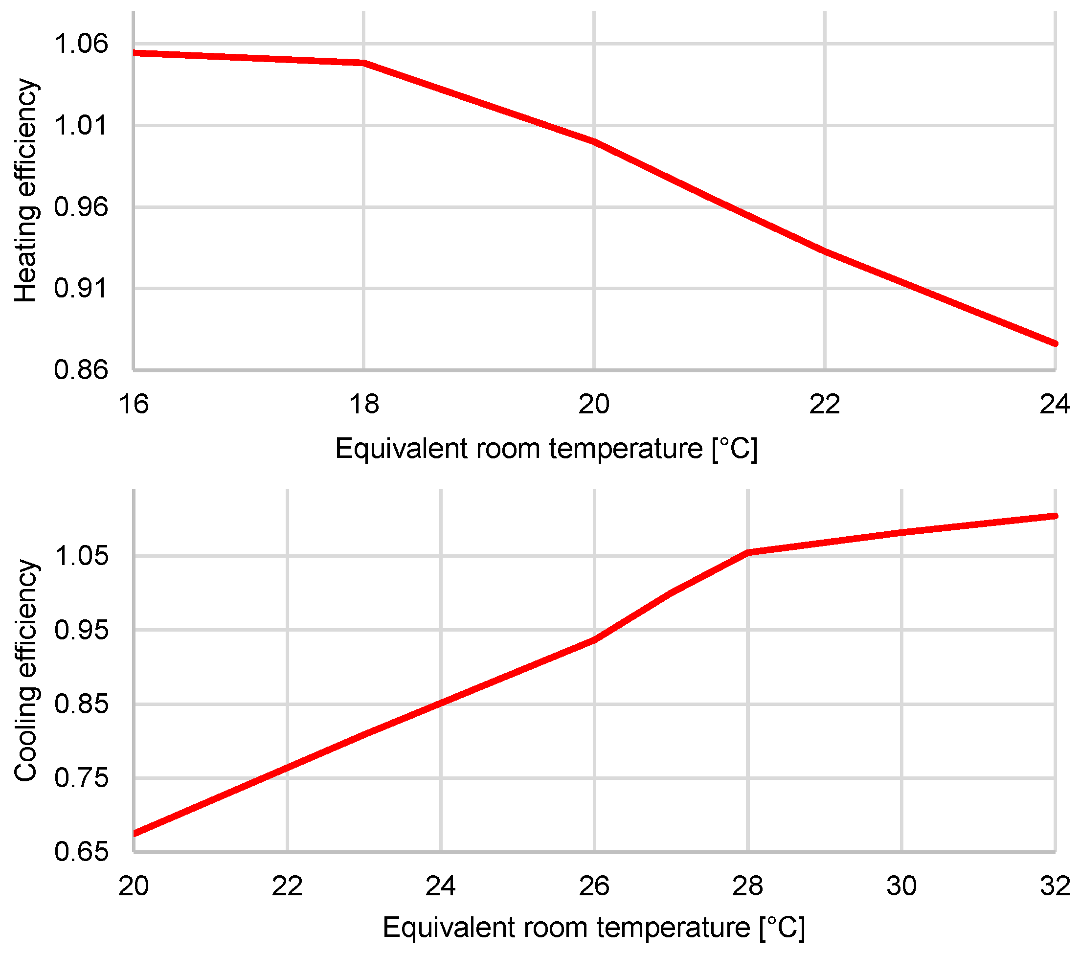
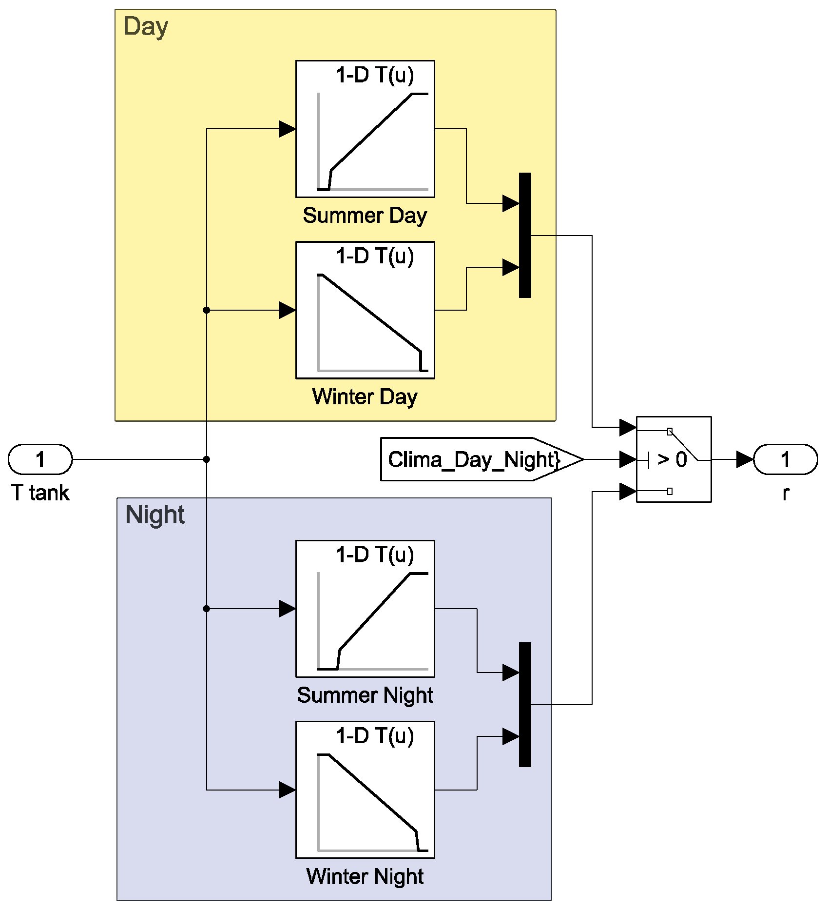
$f\left(•\right)$	non-linear efficiency/room temperature function of a fan coil unit (see Figure 6).
$T_{roo{m}_{eq}}$	computed equivalent room temperature in degrees Celsius.
$T_{room}$	temperature of the air inside the building in degrees Celsius.
$T_{liquid}$	temperature of the liquid inside the coil in degrees Celsius.
$T_{liqui{d}_{ref}}$	reference temperature of the liquid inside the coil (50 °C when heating, 10 °C when cooling).
$P_{el}$	computed amount of electrical power absorbed by the fan coil unit in watts.
$b$	like $a$, but applied to the electrical power absorbed by the unit.
$P_{e{l}_{nom}}$	nominal electrical power rating (in watts) of a unit.
$s$	fan speed setting (Table 3, L0 means that the fan is off).

The electrical power consumed by the fan coil is computed according to the speed of the fan and is absorbed from the campus grid by means of the Power to AC Grid Interface block (Figure 4).

We coupled the building subsystem model (Figure 4) with the heat pump unit subsystem model (Figure 7), which features the following:

• A pair of pipes implementing a lumped model of the thermal liquid circuit.
• A water tank, which is the thermal storage unit of the system.
• Two recirculation pumps.
• A heat exchanger, whereby the thermal power generated by the heat pump is transferred to the thermal liquid.
• A controlled thermal power source connected to the heat exchanger, representing the thermal pump heating action.
• A temperature source for outdoor temperature reference.

The model implemented in Figure 7 consists of two thermal liquid circuits, each with its own Circulating Pump. Circulating Pump 1 pumps water from the tank through a heat exchanger where the water is heated up or cooled down by the heat pump (Power Source), before flowing back into the tank. The heat exchanger is also coupled with the ambient temperature (Tamb Source) to emulate the system thermal losses. The second circuit, driven by Circulating Pump 2, pumps water from the tank through the pipeline that supplies the fan coil unit. The pumps are modeled by means of the Fixed Displacement Pump block from the Simscape library, supplied by an Angular Velocity Source and set at the desired rotating speed. The amount of thermal power provided to the water by the heat pump is computed by the Act. Curves block (Figure 8) and it is proportional to the difference between the water temperature set-point and the actual value of the temperature of the liquid in the tank. The control logic uses different temperature set-point ranges depending on the time of day and on the working days calendar, as shown in

Table 4. Water temperature range thresholds employed in the control of the heat pump unit.

		Season
		Summer	Winter
Mode	Normal	10 ÷ 18 °C	40 ÷ 50 °C
	Quiet	16 ÷ 20 °C	38 ÷ 42 °C

.

The electrical consumption of the heat pump is computed by applying the Energy Efficiency Ratio (EER) and Coefficient of Performance (COP) to the value of generated thermal power, according to the operating mode of the system (cooling or heating). The electrical power value is finally absorbed from the campus grid (AC Grid Interface block in Figure 7).

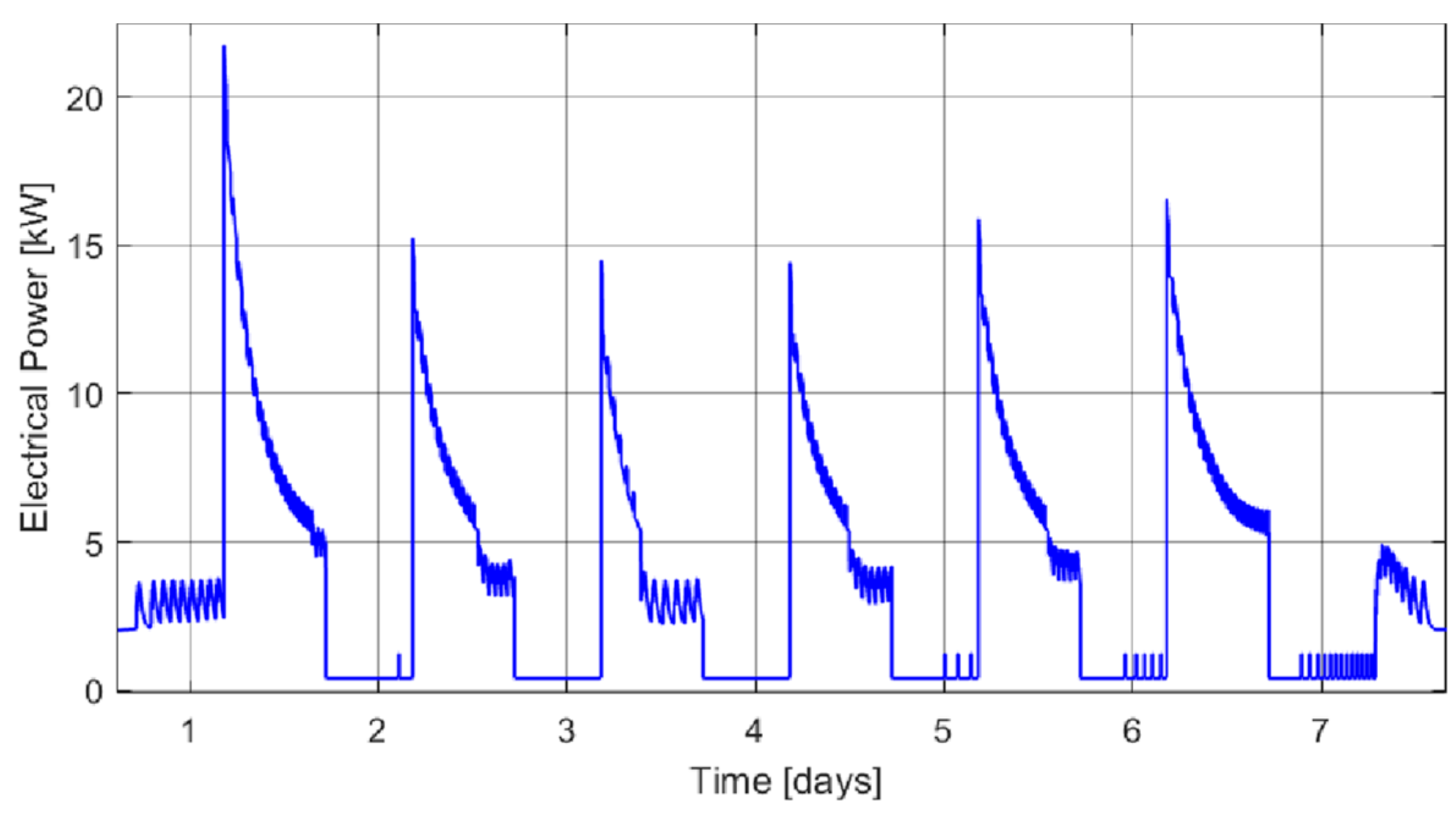
4. Simulation Results

The time dependence of the electrical power consumption of the heating/cooling system displayed in Figure 9 for a sample week in January shows the daily early morning peaks due to the heating pump restoring the liquid to Normal conditions after the nighttime rest, and the intra-day oscillations due to the on-off and step-speed regulation of the fan coil units. The total electrical energy consumption for the air conditioning is about 11 MWh during the first part of the year (heating mode), 5 MWh during the summer period (cooling mode), and 7 MWh during the final part of the year (heating mode), with a global annual consumption of about 23 MWh. Figure 10a shows the details of the power consumption of the conditioning system of the building during an entire sample year, while Figure 10b shows how the temperature of the vector liquid and the amount of thermal power provided by the heat pump to the liquid vary during different periods of the year.

The monthly electrical energy budget for the simulated building is presented in Figure 11. In Figure 11a, we compare the consumption of the air conditioning system (blue circles), the electrical loads (green circles), and the energy production from the PV system (orange squares). It is clear that the photovoltaic production is insufficient to meet the total load demand. However, on average, PV production can satisfy the energy demand of the heat pump air conditioning system over the entire year. In fact, the total photovoltaic production amounts to 28.5 MWh, while the consumption by the air conditioning system is 23.6 MWh.

In

Table 5. Sensitivity of the heating/cooling model to variations in the thermal network parameters.

Heat Transfer Coefficient	Thermal Conductivity	COP	EER	Electrical Energy (Eel)	ΔEel [%]
Table 1	Table 1	3.81	3.20	23.65 MWh/year
+10%	Table 1	3.81	3.20	24.38 MWh/year	+3.1%
Table 1	+10%	3.81	3.20	24.12 MWh/year	+2.0%
+10%	+10%	3.81	3.20	24.89 MWh/year	+5.2%
Table 1	Table 1	+10%	+10%	21.83 MWh/year	−7.68%
+10%	Table 1	+10%	+10%	22.50 MWh/year	−4.83%
Table 1	+10%	+10%	+10%	22.26 MWh/year	−5.86%
+10%	+10%	+10%	+10%	22.97 MWh/year	−2.86%
Table 1	Table 1	−10%	−10%	25.87 MWh/year	+9.38%
+10%	Table 1	−10%	−10%	26.67 MWh/year	+12.78%
Table 1	+10%	−10%	−10%	26.38 MWh/year	+11.56%
+10%	+10%	−10%	−10%	27.23 MWh/year	+15.13%

we show an example of sensitivity analysis where we evaluate how sensitive the electrical power output of the model (E_el) is to variations in key parameters of the building thermal network, namely the heat transfer coefficients, the thermal conductivities and the COP/EER coefficients. Starting from the blueprint specifications for the VisLab building, we varied the parameters by ±10%.

In Figure 11b, we delve into a more detailed balance of the energy dynamics. Here, the focus is on the produced PV energy (orange circles), the total consumption of all loads including the air conditioning (green circles), and the net energy flowing into the PPC from the UPSC grid into the building (blue diamonds); the latter is further broken down into two components: the energy absorbed from the UPSC grid (red circles) and that injected into the UPSC grid (black circles). This detailed breakdown helps us to understand the interaction between the building’s energy consumption, its internal energy production, and its reliance on the UPSC grid. Figure 12 provides a comprehensive annual overview of the electrical breakdown. The PV generation presents a load-matching index of 28.4%, covering the whole air conditioning system energy demand, which represents 23.5% of the total electrical loads. Finally, Figure 13 shows the estimated CO₂ emissions based on the monthly consumption of energy absorbed from the UPSC grid. We considered two scenarios: without PV generation by the VisLab building (Figure 13, orange circles) and with PV generation (Figure 13, blue circles). The emission factor $\left[{\displaystyle \frac{g_{C{O}_2}}{kWh}}\right]$ is calculated using data from the geographical region where the UPSC is located [30] and adjusted according to the amount of renewable energy self-produced within the UPSC. The estimate shows that, on an annual basis, the presence of internal generation from renewable sources can reduce the building’s energy carbon footprint by approximately 47%.

Figure 14 and Figure 15 present comparisons between simulation results and real-world data. Currently, we only have access to monthly data from legacy metering devices, lacking granular field data. Figure 14 compares the simulated PV energy production with actual production on both a monthly and annual basis. Figure 15, on the other hand, contrasts the measured and simulated net electrical energy exchange between the Vislab building and the UPSC grid. In both cases, we observe a good match between the cumulative annual energy shares. Model error metrics corresponding with the data in Figure 14 and Figure 15 (month-by-month relative errors and overall year-round RMSE) are reported in

Table 6. Model error metrics for monthly PV energy production and net building electrical energy consumption.

Month	Error
	PV Energy (Figure 14)	Energy Consumption (Figure 15)
1	8.2%	5.8%
2	10%	14%
3	18%	11%
4	32%	13%
5	35%	1.3%
6	6.6%	17%
7	19%	21%
8	24%	3.8%
9	5.3%	12%
10	9.0%	13%
11	3.8%	1.6%
12	34%	3.7%
RMSE	547 kWh	603 kWh

. It is important to note that the climatic and environmental data (namely, solar irradiance, ambient temperature, wind direction, and speed) used as input for the model are not derived from on-site measurements, but from averaged climatic databases corresponding to the geographical area in which the UPSC is located [31].

The methodology we adopted allows for easy adaptation of the building model to various specific cases. This is due to its standardized smart building features, including grid connectivity, rooftop photovoltaic generation, a heat pump-based climate control system, blueprint-derived thermal network, and a generalized load consumption profile, all of which can be tailored through simple adjustments to case-specific parameters. This means that once the case study is defined, the model can be fully customized by adjusting the numerous available parameters. For example, PV generation can be configured based on specific technology and local climatic and weather data; inverter efficiency curves can also be included, and so on. On the other hand, the building model is fully parameterized both in terms of electrical loads and thermal network (e.g., building thermal exchange coefficients, heating unit thermal efficacy, heat pump COP and EER, etc.). Furthermore, by integrating climate-responsive parameters and load behavior, the model can be recalibrated to accommodate different environmental conditions and energy demands.

Moreover, the proposed model is well-suited for exploring new energy scenarios at both building and district levels, taking into account the gradual introduction and planning of new components (e.g., RES, BESS, etc.). For instance, in [32] the authors demonstrate how the model can be used to optimize the planning of maintenance interventions on PV systems in order to identify the right balance between costs and benefits, while in [16] we study the introduction of PV and BESS, starting from a legacy grid scenario. These applications highlight the versatility of the simulation framework in supporting energy planning, grid integration, and policy development.

A few limitations of our approach—at least as far as the present stage of the research is concerned—are finally worth pointing out here.

-

The use of the constant-frequency discrete-time three-phase phasor-domain approach allowed us to keep the computational overhead within bounds compatible with the calculation of economic and environmental sustainability figures over long periods of time. On the other hand, this simplification prevents the electrical campus model from accounting for AC frequency variation due to changes in power consumption or generation and other non-steady-state phenomena. This is clearly a limitation as far as the simulation of the interaction between the building and the campus micro-grid is concerned.

-

Another significant limitation at the present stage of this activity is the lack of a pervasive metering network able to provide the model with building-specific power data taken at short time intervals. The deployment of metering units has just recently started and it is expected that consistent data collection will start being available in the coming months. This will provide us with the necessary information for evaluating the model’s accuracy and, if necessary, improving it.

-

It is also worth mentioning that we did not set out to develop a Building Energy Management System, so no optimization algorithm is presently included for energy efficiency or cost minimization.

5. Conclusions

In this work, we presented an Integrated Building Energy Modeling (IBEM) approach, developed in the MATLAB environment, to simulate a building that is a representative example of the current trends towards sustainability (increasing electrification and localized energy production by rooftop PV). The model seamlessly integrates dynamic thermal and electrical behaviors by including the heating/cooling system model, photovoltaic generation, and electrical loads into a complete, physical description of the energy performance of a smart building, and is part of the comprehensive MATLAB Simulink electrical model of the University of Parma South Campus micro-grid.

The key results of this work can therefore be summarized as follows:

-

We have developed a MATLAB Simulink IBEM model based on a physical description of all the relevant components, and seamlessly integrated it into our campus micro-grid model;

-

The physical, white-box approach we followed makes it straightforward to apply the building model to different specific instances, given its standard smart building features of grid connection, PV rooftop generation, heat pump-based conditioning system, blueprint-based thermal exchange parameters, and generic load consumption description, with a simple change of case-specific parameter settings;

-

The fact that the whole model (IBEM and micro-grid) is implemented in the MATLAB Simulink environment makes it fully portable and exploitable within the very wide community of MATLAB users, including researchers, utility companies, and educational institutions.

We used the model to obtain a number of simulations describing the detailed energy performance of the building over a whole year, showing its usefulness in the building design and energy assessment phases. The results confirm that the model effectively meets the initial objectives of performing detailed scenario simulations on a monthly and annual timescale providing data about energy behavior, enabling empirical comparisons, and demonstrating strong potential for real-world deployment. Although complete experimental validation is at the present stage hindered by limited availability of field metering data, the comparison between the available experimental data and simulations is encouraging.

Thanks to the adopted approach, while the model is developed and validated within the context of a specific building and climate, its core principles and architecture offer a high degree of adaptability. The modular nature the framework—encompassing energy generation, storage, distribution, and loads—allows for customization to suit various building types. Thus, with appropriate adjustments, it holds significant potential for broader application across diverse contexts and scenarios.

We believe, therefore, the model to represent a useful and effective tool to guide the design of smart/green buildings and plan their construction and integration in campus grids. Practical uses of the model include the design of building energy infrastructure, planning of its evolution and upgrades based on evolving economic and regulatory trends, and the possible contributions of smart/green buildings to surrounding grids. Furthermore, the use of the MATLAB environment can make it a widely available and effective educational tool.

-

Future developments of this activity will follow these directions, in chronological order:

-

The IBEM will be enhanced by the introduction of a BESS;

-

The model validation will increasingly rely on field data coming from a metering network currently under deployment;

-

Algorithms will be introduced to maximize energy efficiency and minimize costs and carbon emissions.

References

1. Cao, J.; Spulbar, C.; Eti, S.; Horobet, A.; Yüksel, S.; Dinçer, H. Innovative Approaches to Green Digital Twin Technologies of Sustainable Smart Cities Using a Novel Hybrid Decision-Making System. J. Innov. Knowl. 2025, 10, 100651. [Google Scholar] [CrossRef]
2. Wang, Y.; Wang, Y.; Ni, J.; Zhang, H. Integration of Smart Buildings with High Penetration of Storage Systems in Isolated 100% Renewable Microgrids. J. Energy Storage 2025, 105, 114633. [Google Scholar] [CrossRef]
3. Kılkış, B.; Çağlar, M.; Şengül, M. Energy Benefits of Heat Pipe Technology for Achieving 100% Renewable Heating and Cooling for Fifth-Generation, Low-Temperature District Heating Systems. Energies 2021, 14, 5398. [Google Scholar] [CrossRef]
4. Herrando, M.; Ramos, A. Photovoltaic-Thermal (PV-T) Systems for Combined Cooling, Heating and Power in Buildings: A Review. Energies 2022, 15, 3021. [Google Scholar] [CrossRef]
5. Zhang, S.; Ocłoń, P.; Klemeš, J.J.; Michorczyk, P.; Pielichowska, K.; Pielichowski, K. Renewable Energy Systems for Building Heating, Cooling and Electricity Production with Thermal Energy Storage. Renew. Sustain. Energy Rev. 2022, 165, 112560. [Google Scholar] [CrossRef]
6. Stamatellos, G.; Zogou, O.; Stamatelos, A. Interaction of a House’s Rooftop PV System with an Electric Vehicle’s Battery Storage and Air Source Heat Pump. Solar 2022, 2, 186–214. [Google Scholar] [CrossRef]
7. Rojek, I.; Mikołajewski, D.; Galas, K.; Piszcz, A. Advanced Deep Learning Algorithms for Energy Optimization of Smart Cities. Energies 2025, 18, 407. [Google Scholar] [CrossRef]
8. Muse, L.P.; Routray, S.; Oleinikova, I. Smart Grids for Smart Cities. IEEE Smart Grid Bulletin 2022. [Google Scholar]
9. Brown, A.; Foley, A.; Laverty, D.; McLoone, S.; Keatley, P. Heating and Cooling Networks: A Comprehensive Review of Modelling Approaches to Map Future Directions. Energy 2022, 261, 125060. [Google Scholar] [CrossRef]
10. Olympios, A.V.; Kourougianni, F.; Arsalis, A.; Papanastasiou, P.; Pantaleo, A.M.; Markides, C.N.; Georghiou, G.E. A Holistic Framework for the Optimal Design and Operation of Electricity, Heating, Cooling and Hydrogen Technologies in Buildings. Appl. Energy 2024, 370, 123612. [Google Scholar] [CrossRef]
11. Bayasgalan, A.; Park, Y.S.; Koh, S.B.; Son, S.-Y. Comprehensive Review of Building Energy Management Models: Grid-Interactive Efficient Building Perspective. Energies 2024, 17, 4794. [Google Scholar] [CrossRef]
12. Hoseinpoori, P.; Olympios, A.V.; Markides, C.N.; Woods, J.; Shah, N. A Whole-System Approach for Quantifying the Value of Smart Electrification for Decarbonising Heating in Buildings. Energy Convers. Manag. 2022, 268, 115952. [Google Scholar] [CrossRef]
13. Causone, F.; Scoccia, R.; Pelle, M.; Colombo, P.; Motta, M.; Ferroni, S. Neighborhood Energy Modeling and Monitoring: A Case Study. Energies 2021, 14, 3716. [Google Scholar] [CrossRef]
14. Sola, A.; Corchero, C.; Salom, J.; Sanmarti, M. Simulation Tools to Build Urban-Scale Energy Models: A Review. Energies 2018, 11, 3269. [Google Scholar] [CrossRef]
15. Simonazzi, M.; Delmonte, N.; Cova, P.; Ferrari, G.; Zanichelli, F.; Menozzi, R. Modeling of a University Campus Micro-Grid for Optimal Planning of Renewable Generation and Storage Deployment. In Proceedings of the 2021 IEEE International Smart Cities Conference (ISC2), Manchester, UK, 7–10 September 2021; IEEE: Piscataway, NJ, USA, 2021; pp. 1–7. [Google Scholar]
16. Simonazzi, M.; Delmonte, N.; Cova, P.; Menozzi, R. Models for MATLAB Simulation of a University Campus Micro-Grid. Energies 2023, 16, 5884. [Google Scholar] [CrossRef]
17. Gambarotta, A.; Morini, M.; Rossi, M.; Stonfer, M. A Library for the Simulation of Smart Energy Systems: The Case of the Campus of the University of Parma. Energy Procedia 2017, 105, 1776–1781. [Google Scholar] [CrossRef]
18. De Lorenzi, A.; Gambarotta, A.; Morini, M.; Rossi, M.; Saletti, C. Setup and Testing of Smart Controllers for Small-Scale District Heating Networks: An Integrated Framework. Energy 2020, 205, 118054. [Google Scholar] [CrossRef]
19. Bianco, G.; Bracco, S.; Delfino, F.; Gambelli, L.; Robba, M.; Rossi, M. A Building Energy Management System Based on an Equivalent Electric Circuit Model. Energies 2020, 13, 1689. [Google Scholar] [CrossRef]
20. Moya, F.; Torres-Moreno, J.; Álvarez, J. Optimal Model for Energy Management Strategy in Smart Building with Energy Storage Systems and Electric Vehicles. Energies 2020, 13, 3605. [Google Scholar] [CrossRef]
21. Khan, M.H.; Asar, A.U.; Ullah, N.; Albogamy, F.R.; Rafique, M.K. Modeling and Optimization of Smart Building Energy Management System Considering Both Electrical and Thermal Load. Energies 2022, 15, 574. [Google Scholar] [CrossRef]
22. Frank, S.; Ball, B.; Gerber, D.L.; Cu, K.; Othee, A.; Shackelford, J.; Ghatpande, O.; Brown, R.; Cale, J. Advances in the Co-Simulation of Detailed Electrical and Whole-Building Energy Performance. Energies 2023, 16, 6284. [Google Scholar] [CrossRef]
23. Alfalouji, Q.; Schranz, T.; Falay, B.; Wilfling, S.; Exenberger, J.; Mattausch, T.; Gomes, C.; Schweiger, G. Co-Simulation for Buildings and Smart Energy Systems—A Taxonomic Review. Simul. Model. Pr. Theory 2023, 126, 102770. [Google Scholar] [CrossRef]
24. Introducing the Phasor Simulation Method. Available online: https://it.mathworks.com/help/physmod/sps/powersys/ug/introducing-the-phasor-simulation-method.html (accessed on 1 August 2022).
25. Song, Y.; Peskova, M.; Rolando, D.; Zucker, G.; Madani, H. Estimating Electric Power Consumption of In-Situ Residential Heat Pump Systems: A Data-Driven Approach. Appl. Energy 2023, 352, 121971. [Google Scholar] [CrossRef]
26. Akbarzadeh, S.; Sefidgar, Z.; Sadegh Valipour, M.; Elmegaard, B.; Arabkoohsar, A. A Comprehensive Review of Research and Applied Studies on Bifunctional Heat Pumps Supplying Heating and Cooling. Appl. Therm. Eng. 2024, 257, 124280. [Google Scholar] [CrossRef]
27. UNI 10077-1; Thermal Performance of Windows, Doors and Shutters—Calculation of Thermal Transmittance. UNI (Italian National Standards Body): Milan, Italy, 2018.
28. UNI 10351; Building Materials—Thermo-Hygrometric Proprieties—Procedure for Determining the Design Values. UNI (Italian National Standards Body): Milan, Italy, 2021.
29. UNI 10355; Chemical Analysis of Ferrous Materials—Inductively Coupled Plasma Optical Emission Spectrometric Analysis of Unalloyed and Low Alloyed Steels—Determination of Si, Mn, P, Cu, Ni, Cr, Mo and Sn, Following Dissolution with Nitric and Sulphuric Acids [Routine Method]. UNI (Italian National Standards Body): Milan, Italy, 2013.
30. The Global Electricity Data Platform. Available online: https://app.electricitymaps.com/zone/IT-NO/72h/hourly (accessed on 14 February 2025).
31. ARPAE Emilia Romagna Dext3r. Available online: https://simc.arpae.it/dext3r/ (accessed on 18 June 2024).
32. Simonazzi, M.; Chiorboli, G.; Cova, P.; Menozzi, R.; Santoro, D.; Sapienza, S.; Sciancalepore, C.; Sozzi, G.; Delmonte, N. Smart Soiling Sensor for PV Modules. Microelectron. Reliab. 2020, 114, 113789. [Google Scholar] [CrossRef]
Figure 1. Building implementation in Simulink.
Energies 18 02948 g001
Figure 2. Normalized weekly power patterns recorded from representative office and research laboratory facilities in (a) a typical week in April (midseason), (b) a typical week in July (summer), and (c) a typical week in December (winter).
Energies 18 02948 g002
Figure 3. Annual consumption profile of the VisLab building obtained by extending and integrating the normalized weekly profiles with monthly consumption trends.
Energies 18 02948 g003
Figure 4. Thermal model of the VisLab building.
Energies 18 02948 g004
Figure 5. Thermostat and Fan Speed Controller subsystem implementation in Simulink model.
Energies 18 02948 g005
Figure 6. Fan coil heat exchange efficiency curves as a function of the equivalent room air temperature for heating (nominal temperature: 20 °C) (top), and cooling (nominal temperature: 27 °C) (bottom). The efficiency is defined to be 1 at the nominal temperature. Data from the manufacturer data sheet.
Energies 18 02948 g006
Figure 7. Model of the heat pump unit with the water tank, the heat exchanger and the circulating pumps. Physical ports 5 and 6 correspond to the same ports in Figure 4: the liquid circulates from the heat pump outlet to the fan coil inlet, then it returns into the water tank.
Energies 18 02948 g007
Figure 8. Details of the implementation of the Act. Curves block (Figure 7).
Energies 18 02948 g008
Figure 9. Power consumption of the air conditioning system of the VisLab building for a week in January.
Energies 18 02948 g009
Figure 10. Example of simulation showing (a) the electrical consumption of the heating/cooling system during an entire year and (b) the temperature of the vector liquid and the amount of thermal power provided by the heat pump to the liquid during different periods of the year.
Energies 18 02948 g010aEnergies 18 02948 g010b
Figure 11. Electrical energy budget for the simulated building: (a) comparison between air conditioning system consumption (blue), electrical loads (green) and PV energy production (orange); (b) detailed balance between produced PV energy (orange), total loads consumption including air conditioning (green) and energy exchange with the UPSC grid (blue); the latter is further split between the energy absorbed from the UPSC grid (red) and that injected into the UPSC grid (black).
Energies 18 02948 g011
Figure 12. Total annual electrical energy breakdown. The PV shows a load-matching index of about 28.4%.
Energies 18 02948 g012
Figure 13. Estimated monthly CO2 emitted by the VisLab building, considering two different scenarios: with (blue) and without (orange) PV rooftop generation. The right axis shows the unit area CO2 emissions.
Energies 18 02948 g013
Figure 14. Comparison of monthly (a) and annual (b) PV energy production results with on-field-measured data.
Energies 18 02948 g014
Figure 15. Comparison of measured and simulated monthly (a) and annual (b) net electrical energy exchange with the UPSC grid.
Energies 18 02948 g015