Investigation of Frequency Response Sharing-Induced Power Oscillations in VSC-HVDC Systems for Asynchronous Interconnection

Abstract

Low-frequency power oscillations (LFPOs) may occur in voltage source converter-based high-voltage direct current (VSC-HVDC) systems when providing frequency support to asynchronously interconnected power grids. This phenomenon has been observed in the LUXI back-to-back (BTB) VSC-HVDC project in China and results from insufficient damping, which may threaten the stability of the overall power system. To better understand and address this problem, this study investigates the root causes of LFPOs and evaluates how different parts of the system affect damping. A combined approach using small-signal modeling and the damping torque method is developed to analyze the damping behavior of DC power in VSC-HVDC systems. Results show that LFPOs are caused by the interaction between VSC-based frequency control and the dynamic response of synchronous generators (SGs). The turbine and governor systems in SGs help stabilize the system by providing positive damping, whereas the DC voltage-controlled VSC station introduces negative damping. The findings are supported by detailed simulations using a modified IEEE 39-bus test system, demonstrating the effectiveness of the proposed analysis method.

1. Introduction

VSC-HVDC systems are considered a flexible and economical solution for long-distance energy transmission [1]. Due to their decoupling capability, synchronous AC grids can be interconnected or isolated through VSC-HVDC systems. This approach offers two key benefits: (1) it eliminates power angle stability issues in large-scale synchronous AC grids, as demonstrated by the separation of the Southern China Power Grid in 2016 [2]; (2) it enhances connectivity between regional AC grids, such as the interconnection between different regional grids in Europe through HVDC systems [3].

Although asynchronous interconnection through VSC-HVDC can limit faults within the disturbed AC grid and prevent fault propagation between connected AC grids, it also introduces a new challenge in the frequency stability of asynchronously interconnected systems [4]. This is because there is no inertia connection, and the constant power model used by VSC-HVDCs restricts the inherent power support between AC grids [5]. Furthermore, with the increasing penetration of renewable energy generators, which inherently have poor frequency control capabilities, and the replacement of traditional synchronous generators, asynchronously interconnected systems exhibit characteristics of low inertia and limited frequency regulation reserves. As a result, power disturbances can lead to larger frequency deviations.

The sharing of frequency response reserves through VSC-HVDC systems has been identified as an effective approach to improving the frequency stability of asynchronously interconnected systems [6,7]. Numerous studies have investigated the design of ancillary frequency controllers for VSC-HVDC systems. The most direct method involves adding a frequency–power (f–P) droop control to the active power control of the VSC-HVDC, adjusting the active power reference value in response to the frequency deviation of the AC grids to provide primary frequency support [8,9,10]. The f–P droop control is easy to implement, highly robust, and has therefore been widely used in practical engineering applications [5]. To avoid the influence of communication link interruptions, a communication-free frequency control method based on frequency–DC voltage (f–V_dc) droop control has been developed [11]. This f–V_dc droop-based frequency deviation information transmission method has also been extended to wind farm-connected VSC-HVDC systems, providing frequency support to the onshore grid [12,13]. In scenarios involving multi-area asynchronous AC grids connected via MTDC systems, a fuzzy logic-based adaptive loop control was proposed in [8] to avoid conflicting actions among VSC stations during frequency control. Similarly, a dual adaptive nonlinear droop control strategy was introduced to enable MTDC systems to provide variable frequency support based on the level of frequency deviation [14].

In recent years, complex control theory and artificial intelligence-based methods have also been investigated. A perturbation-observed-based control scheme was proposed for VSC-HVDC systems to eliminate frequency events in the receiving-end AC system [15]. However, the frequency response of the sending-end AC system was neglected, which is unreasonable in practical situations where both the sending- and receiving-end AC systems have similar equivalent inertia and frequency response reserves. In [16], a machine learning-based frequency control method was proposed that adjusts the DC power of HVDC systems by detecting the level of frequency disturbance through a multivariate random forest regression algorithm.

Since the auxiliary frequency control module changes the stability characteristics of VSC-HVDCs and subsequently affects the overall stability of asynchronously interconnected systems, the stability analysis of VSC-HVDC systems has been widely investigated. The most common approach is to establish a state-space model for the HVDC system and then assess the relationship between the critical oscillation model and the frequency control parameters [17,18,19]. In [20,21], the positive damping contribution to interarea oscillations from HVDC frequency control has been analyzed. In recent years, sub-/super-synchronous frequency oscillations in offshore wind farm-connected HVDC systems have been reported and thoroughly analyzed [12]. It has been concluded that these oscillations are caused by the interaction between the wind generator converter and the AC current control of the HVDC system.

At the same time, POD methods have been widely researched. In [20,22], the frequency control of HVDC systems has been shown to improve the damping of inter-area oscillations in synchronous grids. To suppress inter-area oscillations, a coordinated POD method based on the joint control of active and reactive power in VSC-HVDC systems was proposed in [23]. In [24,25], a coordinated POD method was developed for offshore WFs connected via HVDC systems. In [26], a supplementary control loop was incorporated into the reactive power control loop of VSC-HVDC systems to enhance damping performance under low-inertia operating conditions.

However, the existing literature does not address the DC power oscillations induced by frequency-response sharing control in HVDC systems. In this study, we report an LFPO observed in the practical LUXI BTB HVDC system in China. From the perspective of system operating scenarios and influencing factors, this frequency-response sharing-induced LFPO differs from the DC power oscillations caused by DC voltage oscillations [26] and sub-/super-synchronous frequency oscillations, which typically occur in renewable energy generator-connected HVDC systems. A detailed analysis of this LFPO, based on state-space modeling and the damping torque method, will be presented in Section 4.

The main contributions of this study are summarized as follows:

(1)

A state-space model of the asynchronously interconnected system, incorporating the effects of frequency control in the VSC-HVDC system, is developed. The developed model serves as the foundation for analyzing the damping characteristics of low-frequency power oscillations LFPOs.

(2)

The nature of the LFPO observed in practical HVDC systems originates from the interaction between the frequency controller and the machine dynamic of SGs. The parameters of the frequency control are identified as the primary influencing factors. In addition, the damping contributions from both the turbine and governor of SGs and the DC voltage-controlled VSC station are examined.

The rest of the paper is organized as follows. A detailed report of the LFPO observed in the LUXI BTB HVDC system is presented in Section 2. A state-space model of asynchronously interconnected systems is established in Section 3. Based on the damping torque method, the nature of this LFPO is revealed, and the damping effects from the governor and turbine of SGs, as well as the DC voltage-controlled VSC, are assessed in Section 4. In Section 5, the analysis results are validated through model analysis and EMT simulation. Finally, conclusions and insights derived from this LFPO are summarized in Section 6.

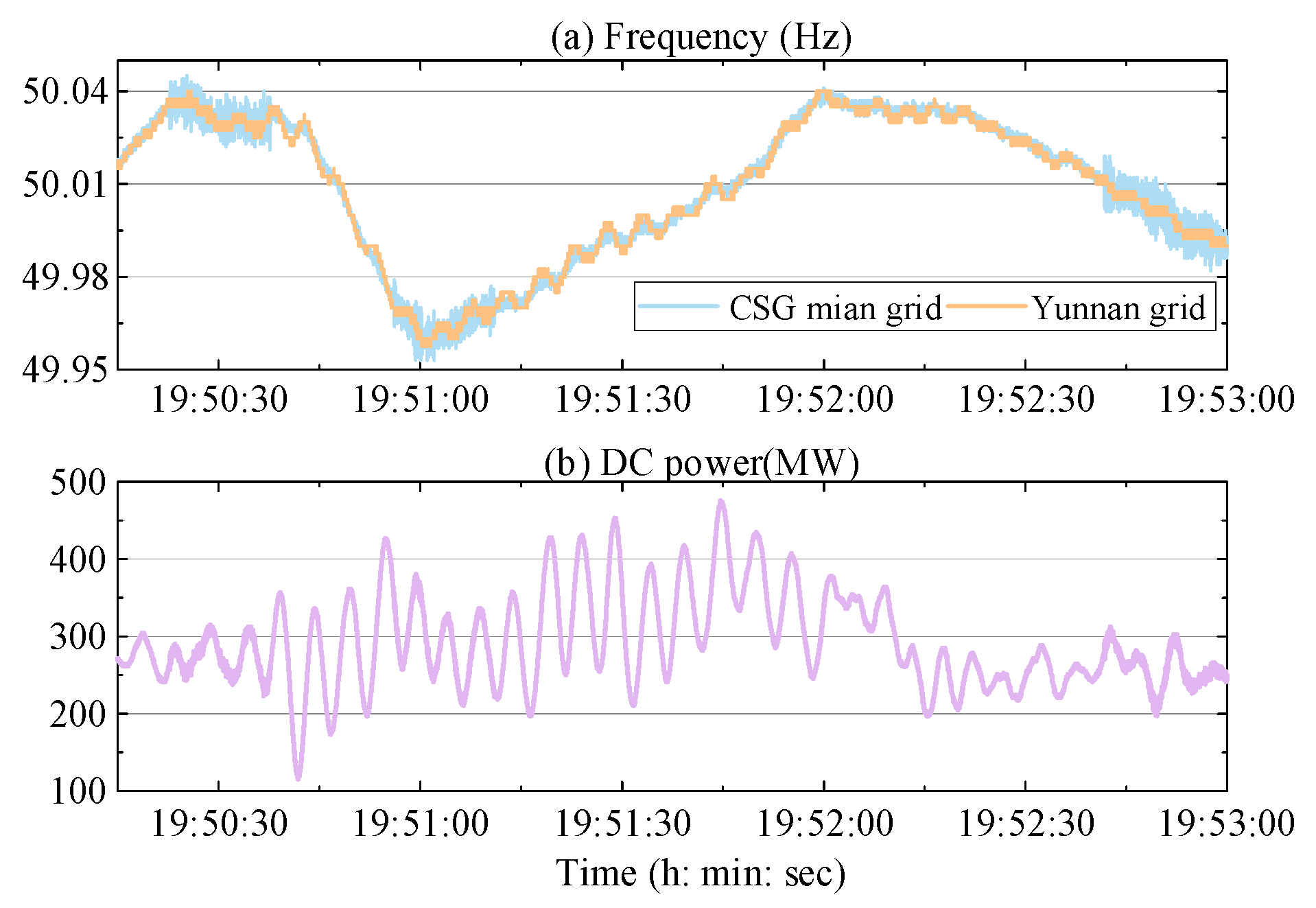
2. LFPO Report

Since the HVDC system operating in constant power mode hinders frequency response reserve sharing between connected asynchronous AC grids, the frequency stability of the Yunnan grid has deteriorated following its asynchronous interconnection from the CSG main grid. The geographical relationship between the Yunnan grid and the CSG main grid is illustrated in Figure 1.

To improve the frequency stability of the Yunnan grid, the co-frequency control, as illustrated in Figure 2, was proposed and incorporated into the active power control loop of the LUXI BTB VSC-HVDC system. This enables real-time frequency response sharing between the Yunnan grid and the CSG main grid. The corresponding mathematical formulation of the co-frequency control will be presented in Section 3.3.

As shown in Figure 3, after the activation of the co-frequency control, the frequencies of the asynchronously interconnected systems are regulated to coincide through the DC power adjustment of the LUXI BTB VSC-HVDC system. However, in certain operational scenarios, a 0.25 Hz low-frequency oscillation has been observed in the DC power of the LUXI BTB VSC-HVDC system, as illustrated in Figure 4. Specifically, Figure 4a shows that during the oscillation period, the frequencies of the asynchronously interconnected systems remain synchronized, while Figure 4b reveals the presence of low-frequency oscillations in the DC power.

Furthermore, as shown in Figure 4a, the frequency deviation of the Yunnan grid and the CSG main grid remains within approximately ±0.04 Hz during the occurrence of the LFPO. This is slightly larger than the frequency deadband of the governors of synchronous generators (SGs) in the CSG main grid (±0.033 Hz), indicating that the governors and turbines of SGs also contribute to the LFPO. Therefore, the damping effect of the governors and turbines on the LFPO should be evaluated. In the next section, a state-space model of the asynchronously interconnected system will be developed, and the damping contribution from each component will be quantitatively determined.

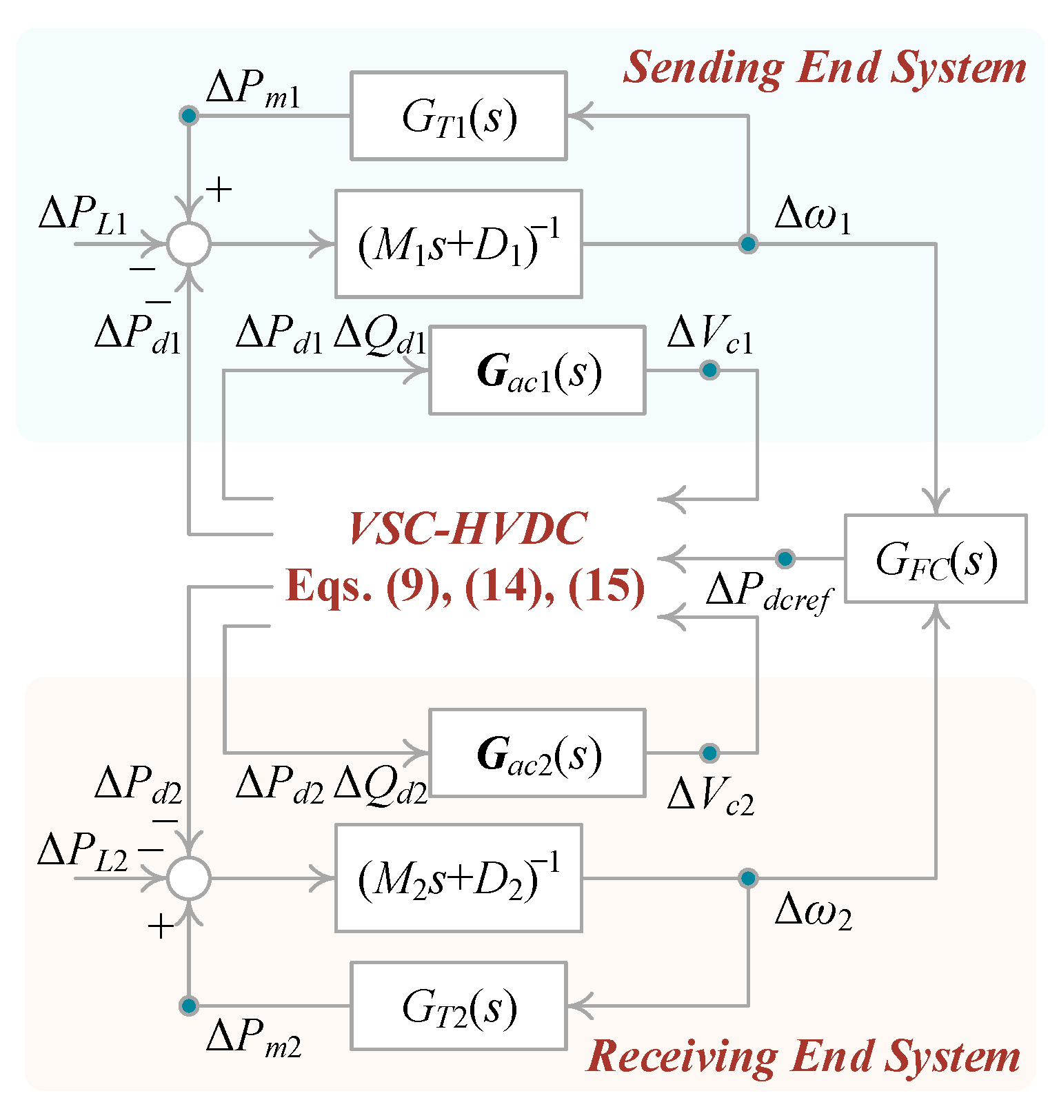
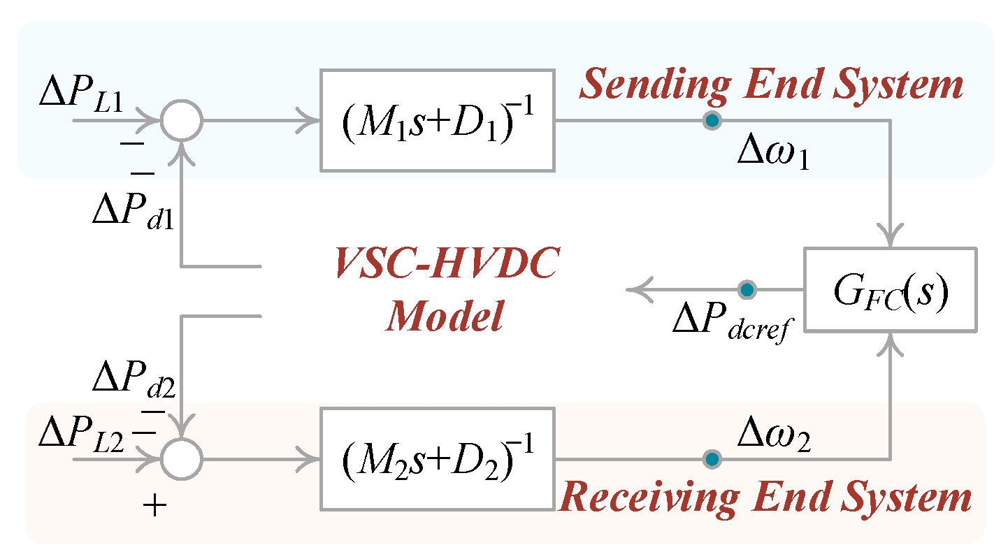
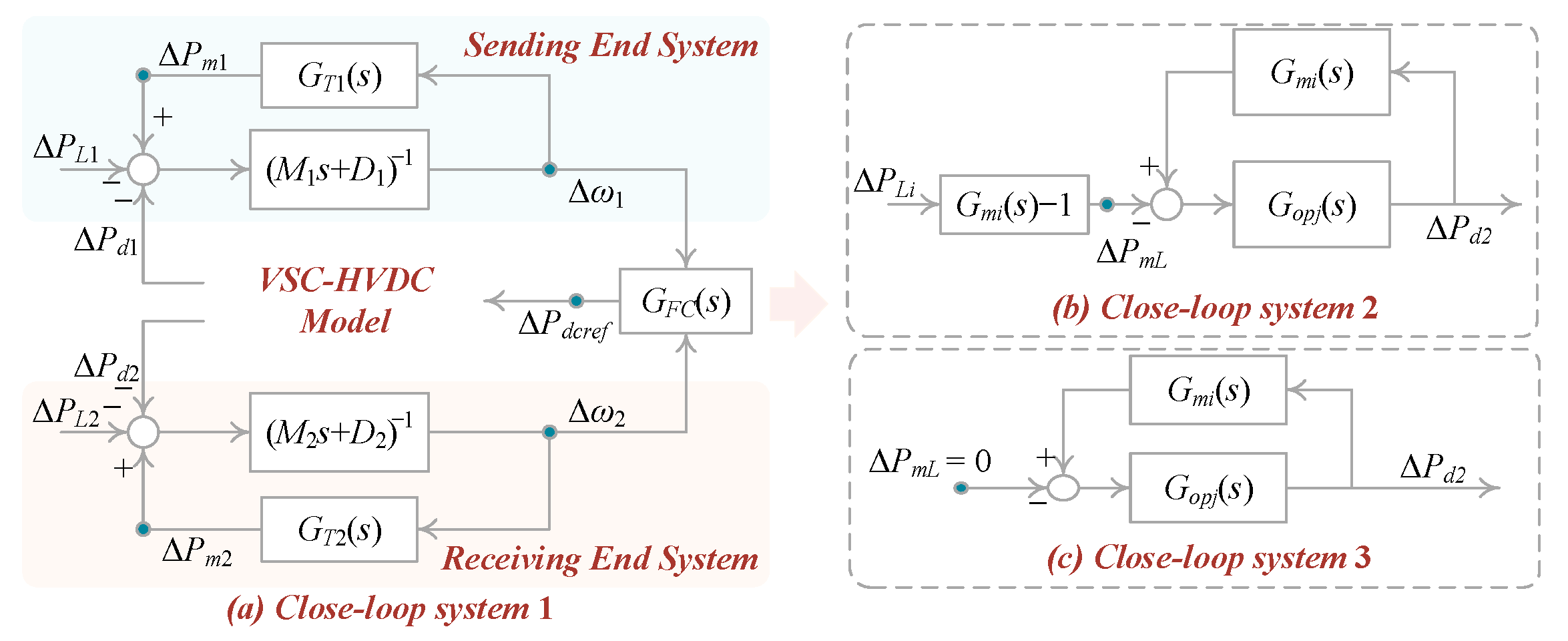
3. System Modeling

In this section, a state-space model of asynchronously interconnected systems incorporating the co-frequency control is established. To facilitate modeling with relative ease, the following assumptions are made:

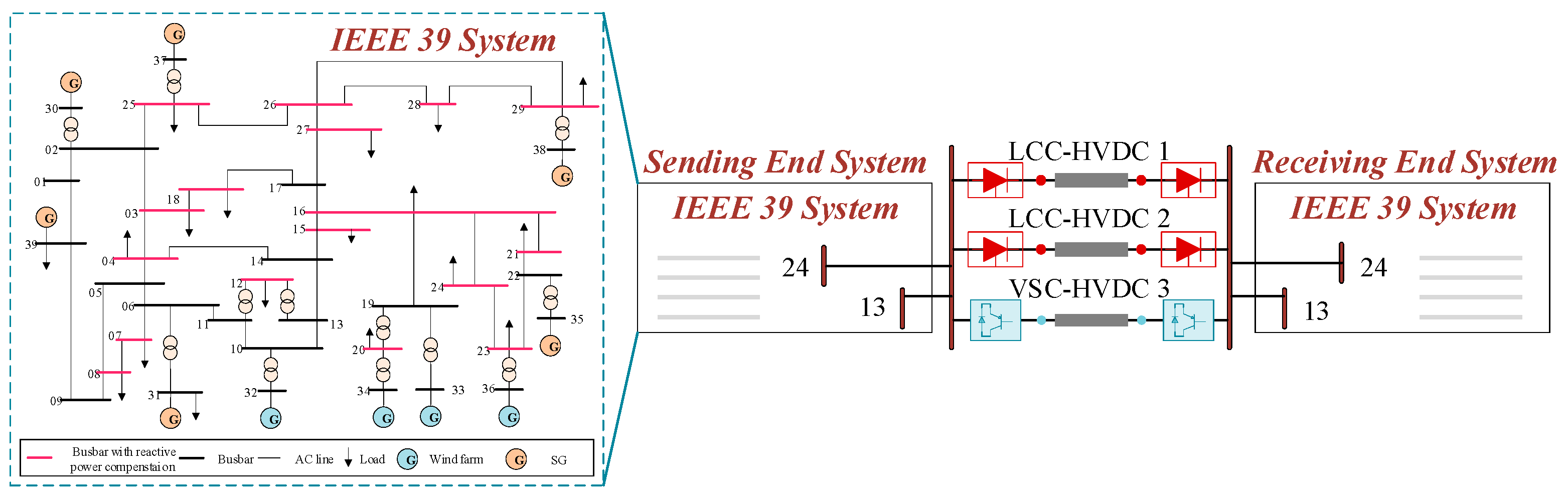
• Two asynchronous grids, i.e., the Yunnan grid and the CSG main grid, are equivalently represented by two SGs, and the AC transmission lines are assumed to be purely inductive.
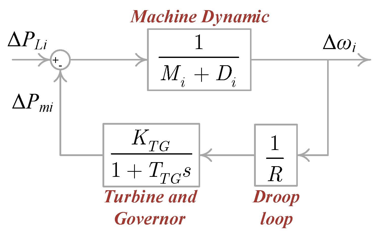
• The damping effects of the machine field circuit, AVR, and PSS are lumped into the damping coefficients D_i.
• The AC voltage at the machine terminal of the SGs is assumed to remain constant, and the frequency response of the SG is only determined by the swing equation, governor, and turbine [26].
• The parallel LCC-HVDC systems are equivalently modeled as constant power loads since these LCC-HVDC systems operate in constant power mode.
• The VSC station is assumed to be lossless, and the inner current control loop is ideal, i.e., i_drefi = i_di.

Based on the above assumptions, the asynchronously interconnected systems illustrated in Figure 1 can be represented as the simplified system shown in Figure 5.

Referring to Figure 5, assuming that the direction of the PCC voltage V_ci is aligned with the d-axis of the VSC d–q coordinate system, i.e., V_cdi = V_ci and V_cqi = 0, the active and reactive power output by the VSCs can be expressed as follows:

$$\left\{\begin{array}{l}{P}_{di}=V_{dci}{I}_{dci}=V_{ci}{i}_{di}\\ Q_{di}=-V_{ci}{i}_{qi}\end{array}\right.,\hspace{1em}i\in \left\{1,2\right\}$$

(1)

where i_di and i_qi are the d–q components of the AC current i_abc, respectively.

For DC side, the dynamics of the DC voltage can be expressed as follows:

$$C_i{\displaystyle \frac{d{V}_{dci}}{dt}}=I_{in1}-{\displaystyle \frac{P_{dci}}{V_{dci}}}$$

(2)

By linearizing (1) and (2), the following can be obtained:

$$\left\{\begin{array}{l}\Delta P_{di}=V_{ci0}\Delta i_{di}+\Delta V_{ci}{i}_{di0}\\ \Delta Q_{di}=-V_{ci0}\Delta i_{qi}-\Delta V_{ci}{i}_{qi0}\end{array}\right.$$

(3)

$$C_i{\displaystyle \frac{d\Delta V_{dci}}{dt}}=\Delta I_{ini}-{\displaystyle \frac{V_{ci0}\Delta i_{di}}{V_{dci0}}}-{\displaystyle \frac{\Delta V_{ci}{i}_{di0}}{V_{dci0}}}+{\displaystyle \frac{I_{dci0}\Delta V_{dci}}{V_{dci0}}}$$

(4)

3.1. Modeling of DC Voltage Controlled-VSC 1

Referring to Figure 5a, the incremental value of the output AC current of VSC 1 can be expressed as follows:

$$\left\{\begin{array}{l}\Delta i_{d1}=\Delta i_{dref1}=(K_{pd1}+K_{id1}{s}^{-1})(\Delta V_{dc1}-\Delta V_{dcref})\\ \Delta i_{q1}=\Delta i_{qref1}=(K_{pq1}+K_{iq1}{s}^{-1})(\Delta Q_{d1}-\Delta Q_{ref1})\end{array}\right.$$

(5)

Typically, the DC voltage reference value V_dcref, the active power reference value P_ref2, and the reactive power reference value Q_refi are set as constant values, resulting in ΔV_dcref = 0 and ΔQ_refi = 0. Defining a state variable Δx₁ = ΔQ_d1/s, the following differential equations can be obtained:

$$\left\{\begin{array}{l}{\displaystyle \frac{d\Delta i_{d1}}{dt}}=K_{pd1}{\displaystyle \frac{d\Delta V_{dc1}}{dt}}+K_{id1}\Delta V_{dc1}\\ (1+V_{c10}{K}_{pq1}){\displaystyle \frac{d\Delta x_1}{dt}}=-V_{c10}{K}_{iq1}\Delta x_1-\Delta V_{c1}{i}_{q10}\end{array}\right.$$

(6)

Combining (4) and (6), the state-space model of the VSC 1 subsystem can be obtained as follows (refer to Appendix A for details):

$$\left\{\begin{array}{l}\Delta {\dot{x}}_{vsc1}=A_{vsc1}\Delta x_{vsc1}+B_{vsc1}\Delta u_{vsc1}\\ \Delta s_{vsc1}=C_{vsc1}\Delta x_{vsc1}+D_{vsc1}\Delta u_{vsc1}\end{array}\right.$$

(7)

where

$$\left\{\begin{array}{l}\Delta x_{vsc1}={\left[\begin{array}{ccc}\Delta i_{d1}& \Delta x_1& \Delta V_{dc1}\end{array}\right]}^T\\ \Delta u_{vsc1}={\left[\begin{array}{cc}\Delta V_{c1}& \Delta I_{in1}\end{array}\right]}^T\\ \Delta s_{vsc1}={\left[\begin{array}{ccc}\Delta P_{d1}& \Delta Q_{d1}& \Delta V_{dc1}\end{array}\right]}^T\end{array}\right.$$

(8)

Based on (7), the open-loop transfer function of the VSC 1 can be obtained as follows [27] (refer to Appendix A for details):

$$\Delta s_{vsc1}=G_{vsc1}(s)\Delta u_{vsc1}=\left[C_{vsc1}{(sI-A_{vsc1})}^{-1}{B}_{vsc1}-D_{vsc1}\right]\Delta u_{vsc1}$$

(9)

3.2. Modeling of Active Power Controlled-VSC 2

Referring to Figure 5b, the incremental value of the output AC current of VSC 2 can be expressed as follows:

$$\left\{\begin{array}{l}\Delta i_{d2}=\Delta i_{dref2}=(K_{pd2}+K_{id2}{s}^{-1})(\Delta P_{dcref}-\Delta P_{dc2})\\ \Delta i_{q2}=\Delta i_{qref2}=(K_{pq2}+K_{iq2}{s}^{-1})(\Delta Q_2-\Delta Q_{ref2})\end{array}\right.$$

(10)

where ΔP_dcref is the incremental active power reference value generated by the co-frequency control and will be presented in the next subsection.

Similarly, the two state variables are defined as Δx₁ = (ΔP_dcref − ΔP_d2)/s and Δx₂ = ΔQ_d2/s. To reduce the number of variables applied, Δx₁ is reused, but this does not affect the system modeling results. The following differential equations can be obtained:

$$\left\{\begin{array}{l}(1+V_{c20}{K}_{pd2}){\displaystyle \frac{d\Delta x_1}{dt}}=-V_{c20}{K}_{id2}\Delta x_1+\Delta P_{dref}-\Delta V_{c2}{i}_{d20}\\ (1+V_{c20}{K}_{pq2}){\displaystyle \frac{d\Delta x_2}{dt}}=-V_{c20}{K}_{iq2}\Delta x_2-\Delta V_{c2}{i}_{q20}\end{array}\right.$$

(11)

Combining (4) and (11), the state-space model of the VSC 2 subsystem can be obtained as follows (refer to Appendix A for details):

$$\left\{\begin{array}{l}\Delta {\dot{x}}_{vsc2}=A_{vsc2}\Delta x_{vsc2}+B_{vsc2}\Delta u_{vsc2}\\ \Delta s_{vsc2}=C_{vsc2}\Delta x_{vsc2}+D_{vsc2}\Delta u_{vsc2}\end{array}\right.$$

(12)

where

$$\left\{\begin{array}{l}\Delta x_{vsc2}={\left[\begin{array}{ccc}\Delta x_1& \Delta x_2& \Delta V_{dc1}\end{array}\right]}^T\\ \Delta u_{vsc2}={\left[\begin{array}{ccc}\Delta P_{dcref}& \Delta V_{c2}& \Delta I_{in2}\end{array}\right]}^T\\ \Delta s_{vsc2}={\left[\begin{array}{ccc}\Delta P_{d2}& \Delta Q_{d2}& \Delta V_{dc2}\end{array}\right]}^T\end{array}\right.$$

(13)

Based on (13), the open-loop transfer function of the VSC 2 can be obtained as follows (refer to Appendix A for details):

$$\Delta s_{vsc2}=G_{vsc2}(s)\Delta u_{vsc2}=\left[C_{vsc2}{(sI-A_{vsc2})}^{-1}{B}_{vsc2}-D_{vsc2}\right]\Delta u_{vsc2}$$

(14)

At the electromechanical time scale, the influence of the equivalent inductance and capacitance of the DC network can be disregarded. Since the LUXI VSC-HVDC is a BTB HVDC system, the mathematical relationship of the DC network can be expressed as follows:

$$\left[\begin{array}{c}\Delta I_{in1}\\ \Delta I_{in2}\end{array}\right]=\left[\begin{array}{cc}-{\displaystyle \frac{1}{R_{dc}}}& {\displaystyle \frac{1}{R_{dc}}}\\ {\displaystyle \frac{1}{R_{dc}}}& -{\displaystyle \frac{1}{R_{dc}}}\end{array}\right]\left[\begin{array}{c}\Delta V_{dc1}\\ \Delta V_{dc2}\end{array}\right]$$

(15)

3.3. Modeling of Asynchronous AC Gird

The transfer function of the frequency–power response of SG can be obtained from Figure 6 as follows [28]:

$$(M_{i}s+D_i+G_{Ti}(s))\Delta {\omega }_i=-\Delta P_{Li}$$

(16)

where ΔP_Li is the difference between mechanical and electrical power. $G_{Ti}={\displaystyle \frac{1}{R}}.{\displaystyle \frac{K_{TG}}{1+T_{TG}s}}$, R is the droop constant, K_TG is the governor constant, and T_TG is the re-heater time constant.

Referring to Figure 2, the incremental active power ΔP_dcref can be expressed as follows:

$$\Delta P_{dcref}=G_{FC}(s)(\Delta {\omega }_1-\Delta {\omega }_2)=(K_{pdc}+K_{idc}{s}^{-1})(\Delta {\omega }_1-\Delta {\omega }_2)$$

(17)

For the AC side, the dynamics of the PCC voltage V_ci in the d–q coordinate system can be expressed as follows:

$$L_i{\displaystyle \frac{d}{dt}}\left[\begin{array}{l}{i}_{di}\\ i_{qi}\end{array}\right]=\left[\begin{array}{l}{V}_{cdi}\\ V_{cqi}\end{array}\right]-\left[\begin{array}{l}{V}_{di}\\ V_{qi}\end{array}\right]-{\omega }_s{L}_i\left[\begin{array}{l}-i_{qi}\\ i_{di}\end{array}\right]$$

(18)

where L_i is the equivalent inductance of the AC transmission line, and ꞷ_s is rated angular frequency (376.99 rad/s or 314.16 rad/s). By substituting (1) into (18) and expressing it in incremental form, the following relationship is obtained:

$$L_i{\displaystyle \frac{d}{dt}}\left[\begin{array}{l}\Delta i_{di}\\ \Delta i_{qi}\end{array}\right]=\left[\begin{array}{l}{\displaystyle \frac{\Delta P_{di}}{i_{di0}}}+{\displaystyle \frac{V_{ci0}\Delta i_{di}}{i_{di0}}}\\ {\displaystyle \frac{-\Delta Q_{di}}{i_{qi0}}}+{\displaystyle \frac{V_{ci0}\Delta i_{qi}}{i_{qi0}}}\end{array}\right]-{\omega }_s{L}_i\left[\begin{array}{c}-\Delta i_{qi}\\ \Delta i_{di}\end{array}\right]$$

(19)

By selecting the state variable $\Delta x_{aci}={[\begin{array}{cc}\Delta i_{di}& \Delta i_{qi}\end{array}]}^T$, input variable $\Delta u_{aci}={[\begin{array}{cc}\Delta P_{di}& \Delta Q_{qi}\end{array}]}^T$, and output variable ΔV_ci, the state-space equation for the AC voltage can be obtained as follows (refer to Appendix A for details):

$$\left\{\begin{array}{l}\Delta {\dot{x}}_{aci}=A_{aci}\Delta x_{aci}+B_{aci}\Delta u_{aci}\\ \Delta V_{ci}=C_{aci}\Delta x_{aci}+D_{aci}\Delta u_{aci}\end{array}\right.$$

(20)

Based on (20), the following transfer function can be obtained:

$$\Delta V_{ci}=G_{aci}(s)\Delta u_{aci}=\left[C_{aci}{(sI-A_{aci})}^{-1}{B}_{aci}-D_{aci}\right]\Delta u_{aci}$$

(21)

As a result, the closed-loop model of the asynchronously interconnected systems, incorporating the VSC-HVDC system with co-frequency control, can be developed based on Equations (9), (14), (16), and (21), as shown in Figure 7.

Based on the developed closed-loop model, the damping analysis of the LFPO will be shown in the next section. Through this analysis, the damping contribution of each component is determined, and the nature of the LFPO is revealed.

4. Damping Analysis

In this section, the frequency response sharing-induced LFPO mode is first identified under ideal prerequisites. It is found that this LFPO is caused by the interaction between the co-frequency control and the machine dynamics of SGs. Next, the damping contributions from other system components-including the DC voltage-controlled VSC 1, the governor and turbine of the SGs, and the SCR of asynchronous AC grids-are independently analyzed using the damping torque method.

4.1. The Nature of the LFPO Mode

Without considering the dynamics of the governor and turbine, and assuming the PCC voltage remains constant (i.e., ΔV_ci = 0) and the VSC-HVDC system is ideal (i.e., ΔP_d1 = −ΔP_d2), the closed-loop model shown in Figure 7 can be simplified as illustrated in Figure 8. Under the above ideal prerequisites, the transfer function of the VSC-HVDC can be simplified and expressed as follows:

$$\Delta P_{d2}=-\Delta P_{d1}={\displaystyle \frac{V_{c20}{K}_{pd2}s+V_{c20}{K}_{id2}}{(1+V_{c20}{K}_{pd2})s+V_{c20}{K}_{id2}}}\Delta P_{dcref}$$

(22)

From (22), it can be observed that the output active power of VSC 2, ΔP_d2, exhibits a first-order response with respect to ΔP_dcref. Since $V_{c20}{K}_{pd2}\gg 1$, the active power response of the VSC 2 can be approximated as ΔP_d2 = ΔP_dcref.

Based on Figure 8, the following mathematical equations can be obtained:

$$\left\{\begin{array}{l}{\displaystyle \frac{d\Delta {\omega }_1}{dt}}={\displaystyle \frac{1}{M_1}}\left(-\Delta P_{L1}-\Delta P_{d1}-D_1\Delta {\omega }_1\right)\\ {\displaystyle \frac{d\Delta {\omega }_2}{dt}}={\displaystyle \frac{1}{M_2}}\left(-\Delta P_{L2}-\Delta P_{d2}-D_2\Delta {\omega }_2\right)\end{array}\right.$$

(23)

$$\Delta P_{d2}=\Delta P_{dcref}=(K_{pdc}+K_{idc}{s}^{-1})\Delta {\omega }_{12}$$

(24)

where $\Delta {\omega }_{12}=\Delta {\omega }_1-\Delta {\omega }_2$. By mathematical transformation, (23) can be rewritten as

$${\displaystyle \frac{d\Delta {\omega }_{12}}{dt}}=-\Delta P_{L12}-M_{12}\Delta P_{d2}-D_{12}\Delta {\omega }_{12}$$

(25)

where

$$\Delta P_{L12}={\displaystyle \frac{\Delta P_{L1}}{M_1}}-{\displaystyle \frac{\Delta P_{L2}}{M_2}}, M_{12}={\displaystyle \frac{1}{M_1}}+{\displaystyle \frac{1}{M_2}}, D_{12}={\displaystyle \frac{D_1}{M_1}}+{\displaystyle \frac{D_2}{M_2}}$$

(26)

Combining (24) and (25), the open-loop transfer function of ΔP_d2 is as follows:

$$\Delta P_{d2}={\displaystyle \frac{K_{pdc}s+K_{idc}}{s^2+(K_{pdc}{M}_{12}+D_{12})s+K_{idc}{M}_{12}}}\Delta P_{L12}$$

(27)

Assuming that ${\lambda }_{m0}=-{\epsilon }_{m0}\pm j{\omega }_{m0}$ is the LFPO mode, it can be calculated from (27) as follows:

$$\begin{array}{l}{\epsilon }_{m0}={\displaystyle \frac{K_{pdc}{M}_{12}+D_{12}}{2}}\\ {\omega }_{m0}={\displaystyle \frac{\sqrt{4K_{idc}{M}_{12}-{(K_{pdc}{M}_{12}+D_{12})}^2}}{2}}\end{array}$$

(28)

From (28), the following conclusions can be made:

(1)

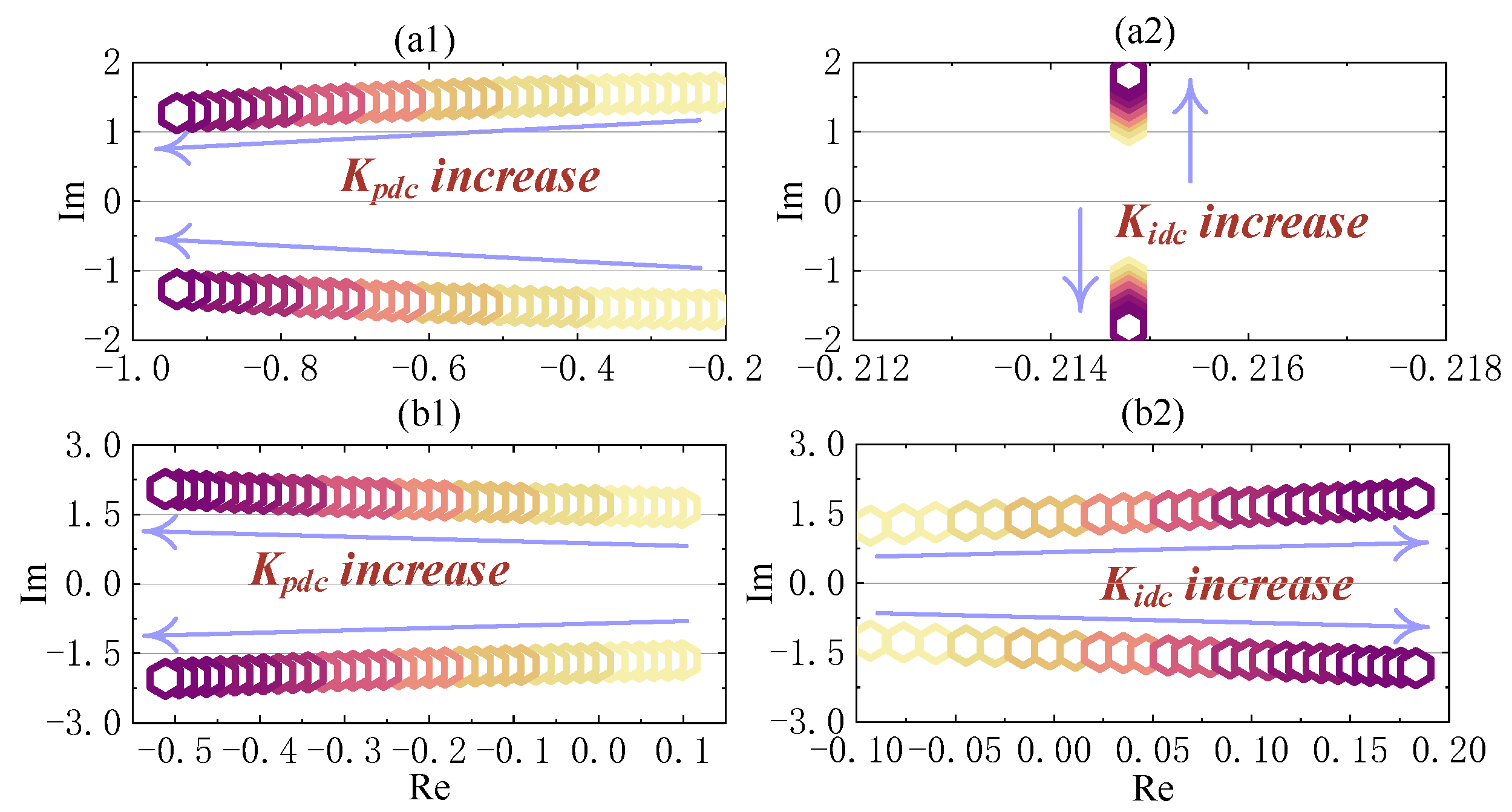
The damping coefficient ${\epsilon }_{m0}$ and angular frequency ${\omega }_{m0}$ of the LFPO mode are determined by the equivalent inertia and damping coefficients of the asynchronously interconnected systems, as well as the proportional and integral gains of the co-frequency control. Since these parameters are related to the SGs at both ends of the AC systems and the co-frequency controller, it can be concluded that this frequency response sharing-induced LFPO is caused by the interaction between the swing dynamics of the SGs and the co-frequency control.

(2)

The damping coefficient of the LFPO mode is positively related to the proportional coefficient K_pdc, and the angular frequency of this mode is positively related to the integral coefficient K_idc. Therefore, by properly increasing K_pdc while decreasing K_idc, the damping ratio of the LFPO model can be effectively improved.

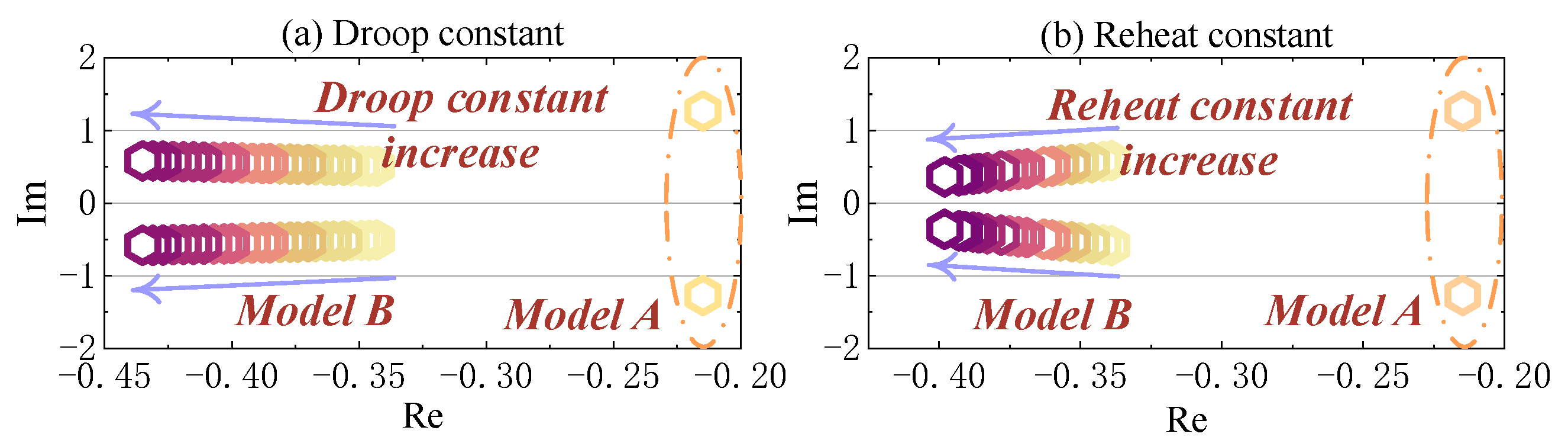
4.2. The Damping Contribution from the Governor and Turbine

Based on the analysis in Section 4.1 and considering the dynamics of the governor and turbine, the closed-loop model shown in Figure 8 can be expanded, as illustrated in Figure 9a. Referring to Figure 9a, ΔP_d2 can be expressed as follows:

$$\begin{array}{l}\Delta P_{d2}={\displaystyle \frac{(K_{pdc}s+K_{idc})\left[(M_{j}s+D_j)(\Delta P_{mi}-\Delta P_{Li})\right]}{s^2+(K_{pdc}{M}_{12}+D_{12})s+K_{idc}{M}_{12}}},i\ne j\in \{1,2\}\\ =G_{opj}(s)(\Delta P_{mi}-\Delta P_{Li})\end{array}$$

(29)

Compared with (27), it is found that $G_{opj}(s)$ denotes the LFPO mode. In addition, ΔP_mi can be expressed as follows:

$$\Delta P_{mi}={\displaystyle \frac{-G_{Ti}(s)(\Delta P_{Li}+\Delta P_{di})}{(M_{i}s+D_i-G_{Ti}(s))}}=G_{mi}(s)(\Delta P_{Li}-\Delta P_{di})$$

(30)

by substituting (30) into (29), the following can be obtained:

$$\Delta P_{d2}=G_{opj}(s)(G_{mi}(s)-1)\Delta P_{Li}-G_{opj}(s)G_{mi}(s)\Delta P_{di}$$

(31)

Based on (31), the closed-loop system shown in Figure 9a can be modified as shown in Figure 9b. From Figure 9b, it can be observed that the effect of the governor and turbine can be classified into two aspects: (1) changing the form of the active power disturbance ΔP_Li; (2) introducing a negative feedback loop $G_{mi}(s)$, thereby affecting the LFPO mode.

To assess the influence of the governor and turbine on the LFPO mode, the closed-loop system shown in Figure 9b can be simplified, as illustrated in Figure 9c. Equation (31) can then be rewritten as follows:

$$\Delta P_{d2}=G_{opj}(s)\Delta P_{mL}-G_{opj}(s)G_{mi}(s)\Delta P_{di}$$

(32)

Assuming that the active power disturbance occurs in the receiving-end system, the characteristic equation of the LFPO can be derived as follows:

$$(s^2+(K_{pdc}{M}_{12}+D_{12})s+K_{idc}{M}_{12}+G_{res1}(s))\Delta P_{d2}=0$$

(33)

where $G_{res1}(s)=(K_{pdc}s+K_{idc})G_{m2}(s)$. Based on the damping torque method, at an angular frequency ꞷ_m, the residue term $G_{res1}(s)$ can be decomposed into two real values, which are proportional to $s\Delta P_{d2}$ and $\Delta P_{d2}$, as follows [29]:

$$G_{res1}(j{\omega }_m)=G_{d1}s+G_{s1}$$

(34)

where

$$G_{d1}=\mathrm{IM}\left[G_{res1}(j{\omega }_m)\right],G_{s1}=\mathrm{Re}\left[G_{res1}(j{\omega }_m)\right]/{\omega }_m$$

(35)

As a result, the LFPO mode ${\lambda }_{m1}=-{\epsilon }_{m1}\pm j{\omega }_{m1}$, considering the damping effect of the turbine and governor, can be calculated as follows:

$$\begin{array}{l}{\epsilon }_{m1}={\displaystyle \frac{K_{pdc}{M}_{12}+D_{12}+G_{d1}}{2}}\\ {\omega }_{m1}={\displaystyle \frac{\sqrt{4(K_{idc}{M}_{12}+G_{s1})-{(K_{pdc}{M}_{12}+D_{12}+G_{d1})}^2}}{2}}\end{array}$$

(36)

From (36), it can be observed that the damping contribution from the governor and turbine can be assessed by calculating the values of G_d1 and G_s1. If G_d1 > 0 and G_s1 < 1, the damping contribution of the governor and turbine is positive. Numerical calculations to determine the values of G_d1 and G_s1 will be shown in Section 5.2, where it will be revealed that the governor and turbine consistently provide a positive damping effect.

4.3. The Damping Contribution from the VSC 1

Based on the analysis in Section 4.1 and considering the dynamics of the VSC 1, the closed-loop model shown in Figure 9 can be expanded, as illustrated in Figure 10a. Referring to Figure 10a, $\Delta P_{d1}$ and $\Delta P_{d2}$ can be derived as follows:

$$\left\{\begin{array}{l}\Delta P_{d1}={\displaystyle \frac{G_{vsc1}^{12}(s)}{1-G_{vsc1}^{11}(s)G_{ac1}(s)}}\Delta I_{in1}=G_{v1}(s)\Delta I_{in1}\\ \Delta P_{d2}={\displaystyle \frac{G_{vsc2}^{11}(s)}{1-G_{vsc2}^{12}(s)G_{ac2}(s)}}\Delta P_{dcref}=G_{v2}(s)\Delta P_{dcref}\end{array}\right.$$

(37)

and the relationship between $\Delta P_{d1}$ and $\Delta P_{d2}$ can be expressed as follows:

$$\Delta P_{d1}={\displaystyle \frac{G_{v1}(s)G_2(s)}{R_{dc}+G_1(s)+G_{vsc2}^{33}(s)}}\Delta P_{d2}=G_v(s)\Delta P_{d2}$$

(38)

Based on (37) and (38), the closed-loop system shown in Figure 10a can be modified into the form shown in Figure 10b. Furthermore, the closed-loop system in Figure 10b can be aggregated into a single-input, single-output (SISO) system, as depicted in Figure 11.

Referring to Figure 11, the characteristic equation of $\Delta P_{d2}$ can be derived as follows:

$$(s^2+(K_{pdc}{M}_{12}+D_{12})s+K_{idc}{M}_{12}+G_{res2}(s))\Delta P_{d2}=0$$

(39)

where

$$G_{res2}(s)=(K_{pdc}s+K_{idc})(G_{fd1}(s)+G_{fd2}(s))$$

(40)

Similarly, based on the damping torque method, Equation (39) can be rewritten as follows:

$$(s^2+(K_{pdc}{M}_{12}+D_{12}+G_{d2})s+K_{idc}{M}_{12}+G_{s2})\Delta P_{d2}=0$$

(41)

where

$$G_{d2}=\mathrm{IM}\left[G_{res2}(j{\omega }_m)\right],G_{s2}=\mathrm{Re}\left[G_{res2}(j{\omega }_m)\right]/{\omega }_m$$

(42)

As a result, the LFPO mode ${\lambda }_{m2}=-{\epsilon }_{m2}\pm j{\omega }_{m2}$ can be calculated as follows:

$$\begin{array}{l}{\epsilon }_{m2}={\displaystyle \frac{K_{pdc}{M}_{12}+D_{12}+G_{d2}}{2}}\\ {\omega }_{m2}={\displaystyle \frac{\sqrt{4(K_{idc}{M}_{12}+G_{s2})-{(K_{pdc}{M}_{12}+D_{12}+G_{d2})}^2}}{2}}\end{array}$$

(43)

From (43), it can be observed that the damping contribution from the VSC 1 and reactive power control of VSCs can be assessed by calculating the values of G_d2 and G_s2. Numerical calculations to assess the values of G_d2 and G_s2 will be shown in Section 5.2.

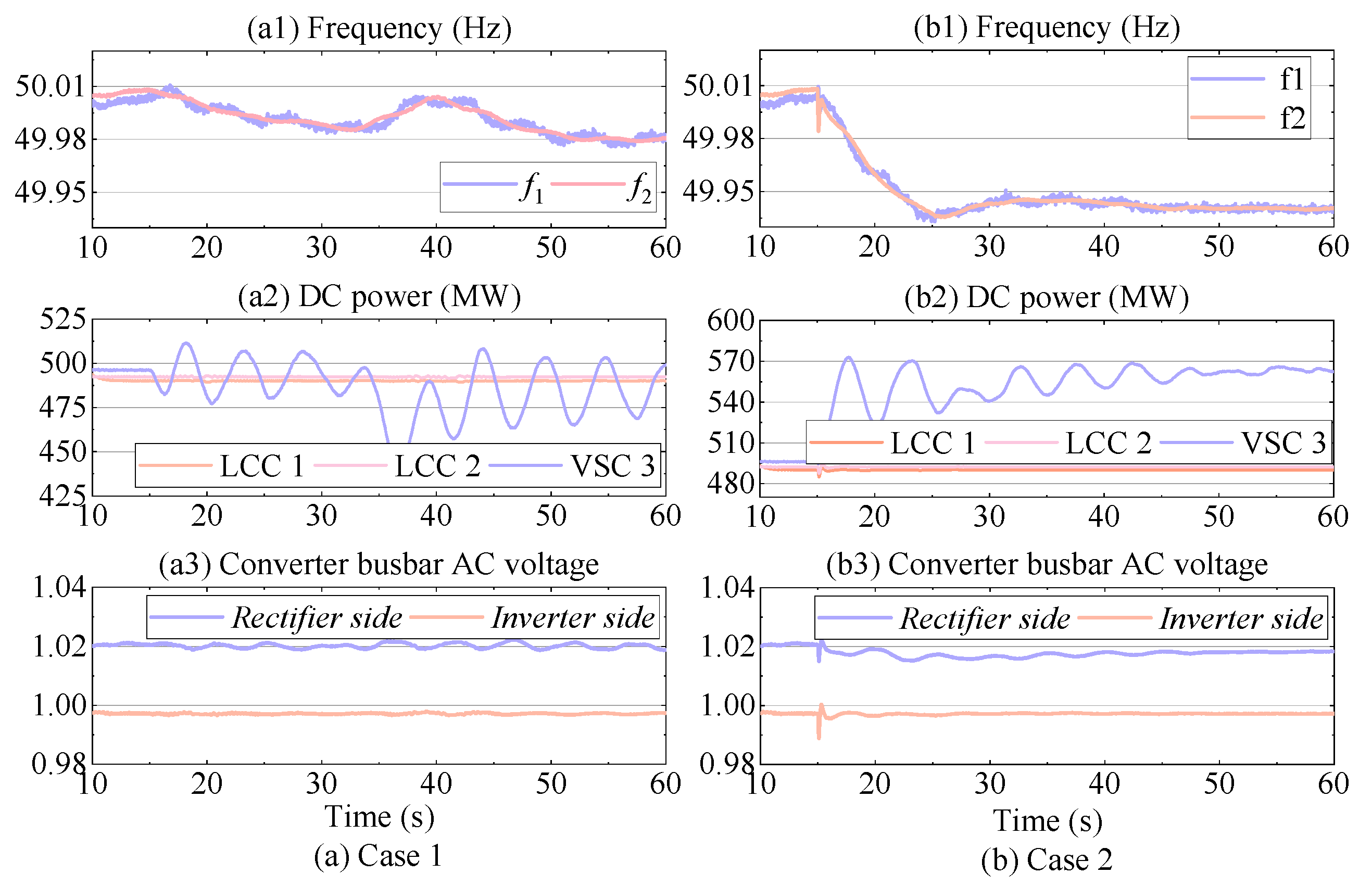
5. Simulation Validation

In this section, an asynchronously interconnected test system is developed using PSCAD/EMTDC V5.0, and the phenomenon of LFPO is successfully reproduced. The effectiveness of the closed-loop model, as shown in Figure 8, is then validated by comparing its results with those of the EMT model. Based on extensive numerical calculations and EMT simulations, the damping contributions from the governor and turbine, as well as the DC voltage-controlled VSC, are identified.

5.1. LFPO Replication

The test system used in this study is modified from the IEEE 39-bus test system to validate the effectiveness of the developed closed-loop system shown in Figure 8, as well as the analysis conclusions. Based on the topology presented in Figure 12, the EMT simulation model used in this study is constructed in PSCAD. To verify the correctness of the EMT model, two simulation cases are conducted to replicate the DC power oscillation phenomenon observed in a real HVDC project. The parameters of the test system are presented in the Appendix A.

In Case 1, the output active power of the WFs is set to change continuously, causing variations in the frequencies of asynchronously interconnected systems. The co-frequency control is implemented in VSC-HVDC link 3 and activated at t = 15.0 s.

In Case 2, a 150 MW step load increase at Bus 19 of the receiving-end system is simulated at t = 15 s. The co-frequency control is implemented in VSC-HVDC link 3 and activated at t = 15.0 s.

Figure 13 shows the simulation results of the test system presented in Figure 12. The left column (Figure 13(a1–a3)) presents the results for Case 1, while the right column (Figure 13(b1–b3)) shows the results for Case 2. As illustrated in Figure 13(a1,b1), once the co-frequency control is activated, the VSC-HVDC system flexibly adjusts the DC power to synchronize the frequencies of the two asynchronous grids. Meanwhile, the DC power of the LCC-HVDC links remains unchanged, as shown in Figure 13(a2,b2). The LFPO is successfully reproduced in Figure 13(a2,b2), exhibiting an oscillation frequency of approximately 0.25 Hz, which is consistent with the oscillation observed in the LUXI BTB VSC-HVDC system.

Furthermore, as displayed in Figure 13(a3,b3), the simulation results closely match the recorded waveforms in Figure 4. This consistency confirms that the test system developed in this study accurately captures the dynamics of the LUXI BTB HVDC system, making it a reliable platform for validating the analysis conclusions.

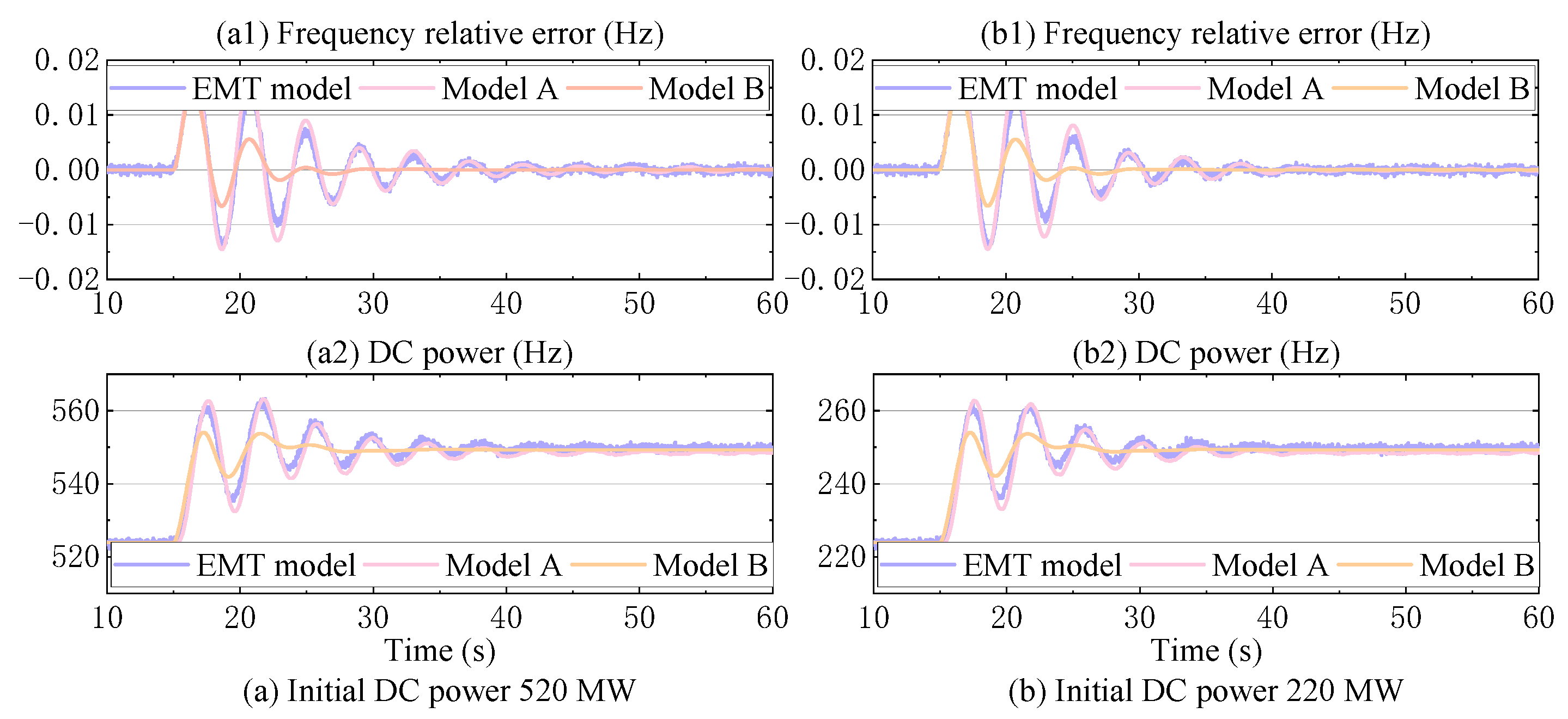
5.2. Model Validation and Parameters Effect Analysis

To verify the accuracy of the developed model in Figure 8, the calculation results of the frequency relative error and DC power from the closed-loop model are compared with the EMT simulation results. Figure 14 displays the comparison of the frequency relative error and DC power under two different initial DC power levels. The closed-loop models in Figure 8 and Figure 9 are used for comparison with the EMT model. In Figure 14, the closed-loop model in Figure 8 is labeled as Model A, while the one in Figure 9 is labeled as Model B.

As illustrated in Figure 14, the calculation results of Model A closely align with the EMT model simulation outcomes, confirming the accuracy of the closed-loop model presented in Figure 8. In contrast, Model B exhibits enhanced damping of the DC power, suggesting that the remaining system components introduce a negative damping effect on the LFPO mode. Consequently, the subsequent section evaluates the damping contributions of the turbine and governor, VSC 1, and grid strength. The analysis reveals that, while the turbine and governor continue to provide a positive damping effect, VSC 1 introduces a negative damping influence.

Given that the co-frequency control parameters (i.e., K_pdc and K_idc) have been identified as the primary factors influencing the LFPO mode, a comprehensive eigenvalue analysis is performed for both Model A and Model B under various co-frequency control parameter settings. This analysis aims to provide deeper insights into the impact of K_pdc and K_idc on system stability and oscillation characteristics. The corresponding eigenvalue loci are presented in Figure 15. In Figure 15, K_pdc varies from 300 to 750 with an increment of 10 while K_idc is set to 600, and K_idc varies from 200 to 500 with an increment of 10, with K_pdc set to 150.

As shown in Figure 15(a1,b1), with an increase in K_pdc, the LFPO modes in both Model A and Model B shift towards the left side of the complex plane. This observation is consistent with the analytical conclusion that increasing K_pdc enhances the damping ratio of the LFPO mode. In contrast, in Figure 15(a2,b2), as K_idc increases, the angular frequency of the LFPO mode in Model A increases, and the mode shifts towards the right side of the complex plane. Both trends indicate that increasing K_idc leads to a reduction in the damping ratio of the LFPO mode.

Moreover, to evaluate the impact of the initial DC power level, the corresponding eigenvalue loci are presented in Figure 16. In this figure, the initial DC power Pdc20 varies from −800 MW to 800 MW in increments of 100 MW. As shown in Figure 16, the LFPO mode in Model A remains unaffected by changes in P_dc20, whereas the LFPO mode in Model B is slightly influenced. These results suggest that the initial DC power level is not a critical influencing factor for the LFPO mode.

5.3. Damping Analysis Validation

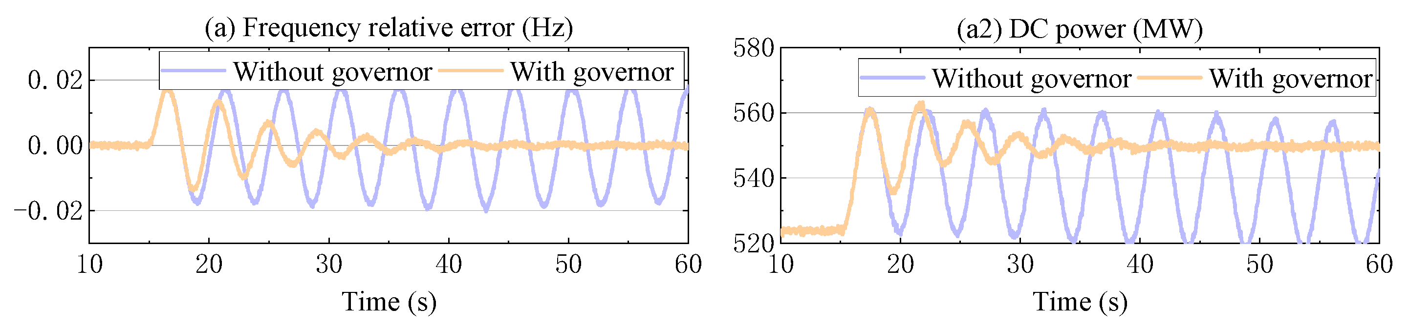
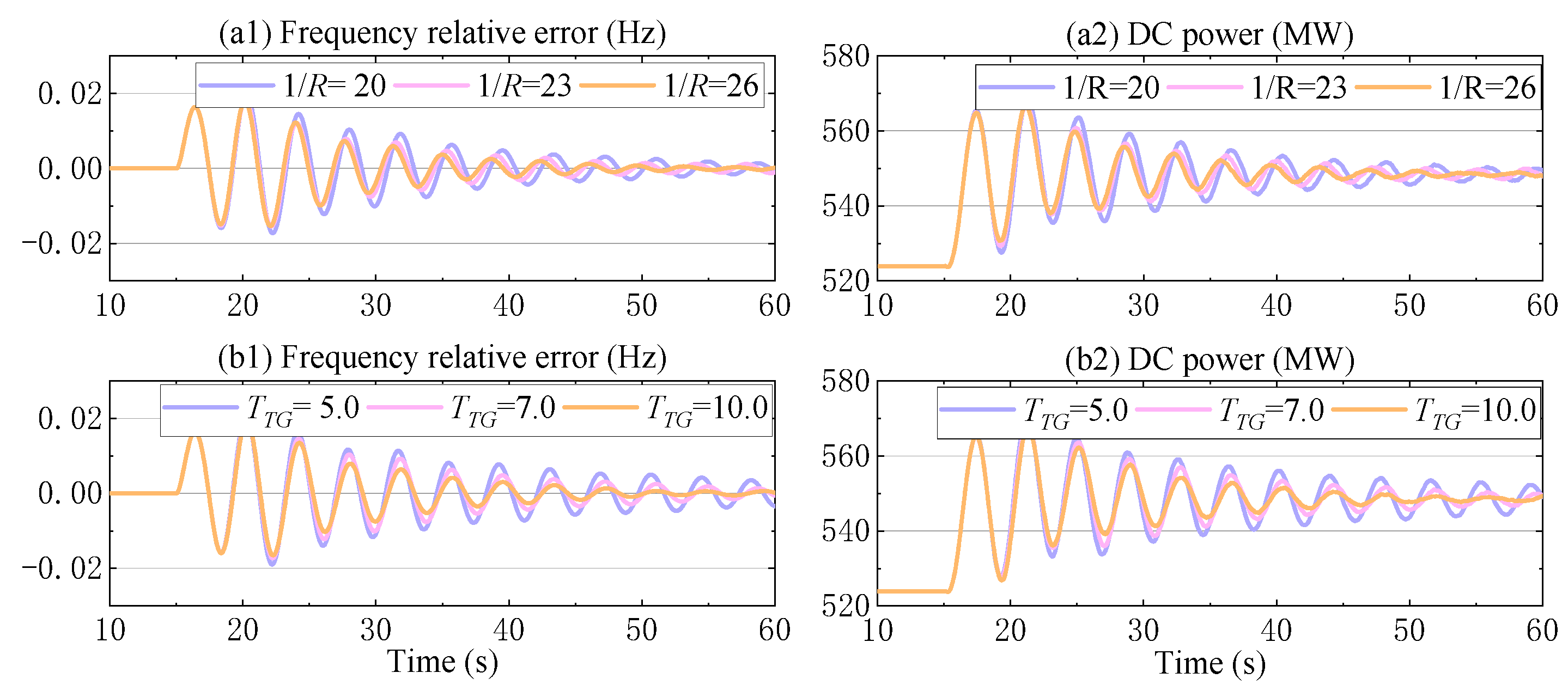
5.3.1. Damping Effect of Turbine and Governor

To assessing the damping contribution from the turbine and governor, the dynamics of the HVDC system are disregarded (i.e., $\Delta P_{dcref}=\Delta P_{d2}=-\Delta P_{d1}$), and the AC voltage at each busbars are assumed to be constant (i.e., $\Delta V_i=\Delta V_{ci}=0$). Based on the model shown in Figure 10a, mode analysis was first conducted. The complex eigenvalues of the DC power oscillation mode in the closed-loop system, as depicted in Figure 9 (Model A) and Figure 10 (Model B), are calculated and presented in Figure 17. In Figure 17, the parameter 1/R varies from 20 to 25 in increments of 0.2, and T_TG varies from 5 to 9 in increments of 0.2, with K_pdc and K_idc fixed at 300 and 1200, respectively.

As shown in Figure 17, the LFPO mode in Model B exhibits better damping characteristics compared to that in Model A, indicating that the governor and turbine contribute a positive damping effect. Moreover, as the droop constant (1/R) and the reheat time constant increase, the positive damping contribution of the governor and turbine becomes more pronounced.

The positive damping contribution of the turbine and governor to the LFPO mode is further verified through frequency sweep analysis. Based on (38), the frequency sweeping results of G_d1 and G_d2 over the frequency range from ω_min = 1.0 rad/s to ω_max = 4.0 rad/s are calculated and presented in Figure 18. As shown in Figure 18, under different values of 1/R and T_TG, G_d1 consistently remains greater than zero, while G_s1 remains less than zero, which is consistent with the results shown in Figure 17.

To validate the analysis, EMT simulations were conducted. Firstly, two scenarios were compared: SGs with and without the governor and turbine. In the scenario without the governor and turbine, the machine torque of the SGs remained unchanged after an active power disturbance is applied. The simulation results for the frequency relative error and DC power are presented in Figure 19. As shown in the figure, the DC power oscillation exhibits improved damping when the turbine and governor are activated, thereby validating the analysis presented in Figure 17 and Figure 18.

Next, the effect of governor and turbine parameters is validated through simulation. In this case, the droop constant and the reheat time constant are varied for comparison, and the corresponding simulation results are presented in Figure 20. As shown in Figure 20(a1,a2), increasing the droop constant leads to a slight improvement in the damping of the DC power oscillation. Similarly, as shown in Figure 20(b1,b2), increasing the reheat time constant also enhances the damping of the DC power oscillation.

5.3.2. Damping Effect of the VSC 1

To assess the damping contribution from the VSC 1, the dynamics of the governor and turbine were neglected. Based on the model shown in Figure 9 and Figure 11, a mode analysis was first conducted. The complex eigenvalues of the LFPO mode in the closed-loop system, as depicted in Figure 9 (Model A) and Figure 11 (Model B), were calculated and presented in Figure 21. In Figure 21, the SCR of the RE and SE AC systems varies from 2.0 to 5.0 in increments of 0.1, respectively. In this case, K_pdc and K_idc were set to 300 and 1200, respectively.

As shown in Figure 21, the LFPO mode in Model A exhibits better damping characteristics than that in Model B, indicating that VSC1 introduces a negative damping effect on the LFPO mode. This negative damping is influenced by the SCRs of both the SE and RE AC systems. As the SCRs increase, the LFPO mode in Model B shifts further to the left in the complex plane, approaching the location of the mode in Model A. This behavior is expected, as a higher SCR leads to a stiffer AC system, resulting in reduced voltage fluctuations at the PCC and, consequently, a weaker influence from AC voltage disturbances.

The positive damping contribution of the VSC 1 to the LFPO mode is further verified through a frequency sweep analysis. Based on (A8), the frequency sweeping results of G_d2 and G_s2 over the frequency range from ω_min = 1.0 rad/s to ω_max = 4.0 rad/s are calculated and presented in Figure 22. As shown in Figure 22, under varying SCR values, G_d2 remains negative while G_s2 remains positive across the frequency range, which is consistent with the modal analysis results shown in Figure 21.

To validate the analytical results, EMT simulations were carried out. Two simulation scenarios were considered: (1) the SCR of the SE AC system was varied while the SCR of the RE AC system was fixed at 5.0; (2) the SCR of the RE AC system was varied while the SCR of the SE AC system was fixed at 5.0. The corresponding simulation results are presented in Figure 23.

As shown in Figure 23(a1,a2), as the SCR of the SE AC system increases, the damping of the DC power oscillation is enhanced. This observation is consistent with the modal analysis and frequency sweep results. A similar dynamic behavior is observed in Figure 23(b1,b2), where an increase in the SCR of the RE AC system also leads to improved damping of the DC power oscillation.

5.4. Discussion

Based on the developed closed-loop model, the root cause of the observed LFPO was first identified. The interaction between the co-frequency controller and the dynamic behavior of SGs is determined to be the underlying mechanism of the LFPO, with K_pdc and K_idc identified as the primary influencing factors.

Under appropriate assumptions and by applying the damping torque method, it is found that the governor and turbine consistently contribute positive damping to the LFPO mode, whereas VSC 1 introduces a negative damping effect. Moreover, the DC power oscillation can be effectively mitigated by optimizing the parameters of the co-frequency controller. In addition, supplementary damping control strategies can be incorporated to further enhance the damping of DC power oscillations. This will be explored as part of the future work of this study.

In practical HVDC engineering, the co-frequency control parameters (e.g., K_pdc and K_idc) tuning process is typically carried out based on the following four steps:

• Determine the system operating conditions, including the equivalent system inertia, damping coefficient, short-circuit ratio (SCR), and HVDC system parameters.
• Predefine the desired damping ratio of the DC power oscillation mode, typically within the range of 0.3 to 0.7, to balance control responsiveness and system stability performance.
• Calculate the feasible range of control parameters based on Equations (28), (36), and (43), such that the resulting damping ratio of the DC power oscillation mode falls within the predefined range.
• Verify the calculated control parameters through time-domain simulations to ensure that the system response meets the expected performance criteria.

6. Conclusions

In this paper, a new type of LFPO, observed in a practical HVDC project in the China Southern Power Grid, is reported and successfully replicated through EMT simulations. By combining the damping torque method with a developed small-signal model, the root cause of the LFPO is identified as the interaction between the co-frequency controller of the VSC-HVDC system and the machine dynamics of SGs in the AC grid. The proportional and integral gains of the co-frequency controller are determined to be the primary influencing factors. It is shown that appropriately increasing K_pdc and decreasing K_idc can effectively enhance the damping ratio of the LFPO mode.

Moreover, the governor and turbine of SGs are found to consistently provide a positive damping contribution to the LFPO mode. This positive contribution is positively correlated with both the droop constant and the reheat time constant. In contrast, the DC voltage-controlled VSC (VSC1) consistently contributes negative damping to the LFPO mode, and this negative contribution becomes more pronounced as the SCR of the connected AC systems decreases. Furthermore, the magnitude of the negative damping contribution from VSC1 is observed to exceed the positive damping provided by the governor and turbine. Given that HVDC systems play a vital role in maintaining frequency stability in asynchronously interconnected systems, this study provides valuable insights for enhancing the functional capabilities of HVDC systems in grid-support applications.

References

- Li, Y.; Tang, G.; An, T.; Pang, H.; Wang, P.; Yang, J.; Wu, Y.; He, Z. Power Compensation Control for Interconnection of Weak Power Systems by VSC-HVDC. IEEE Trans. Power Deliv. 2017, 32, 1964–1974. [Google Scholar]
- Zhou, B.; Rao, H.; Wu, W.; Wang, T.; Hong, C.; Huang, D.; Yao, W.; Su, X.; Mao, T. Principle and Application of Asynchronous Operation of China Southern Power Grid. IEEE J. Emerg. Sel. Top. Power Electron. 2018, 6, 1032–1040. [Google Scholar]
- de Haan, J.E.; Concha, C.E.; Gibescu, M.; van Putten, J.; Doorman, G.L.; Kling, W.L. Stabilising system frequency using HVDC between the Continental European, Nordic, and Great Britain systems. Sustain. Energy Grids Netw. 2016, 5, 125–134. [Google Scholar]
- Obradovic, D.; Dijokas, M.; Misyris, G.S.; Weckesser, T.; Van Cutsem, T. Frequency Dynamics of the Northern European AC/DC Power System: A Look-Ahead Study. IEEE Trans. Power Syst. 2022, 37, 4661–4672. [Google Scholar] [CrossRef]
- Rao, H.; Wu, W.; Mao, T.; Zhou, B.; Hong, C.; Liu, Y.; Wu, X. Frequency control at the power sending side for HVDC asynchronous interconnections between Yunnan power grid and the rest of CSG. CSEE J. Power Energy Syst. 2020, 7, 105–113. [Google Scholar]
- Yan, K.; Li, G.; Zhang, R.; Xu, Y.; Jiang, T.; Li, X. Frequency Control and Optimal Operation of Low-Inertia Power Systems with HVDC and Renewable Energy: A Review. IEEE Trans. Power Syst. 2024, 39, 4279–4295. [Google Scholar]
- Misyris, G.S.; Tosatto, A.; Chatzivasileiadis, S.; Weckesser, T. Zero-Inertia Offshore Grids: N-1 Security and Active Power Sharing. IEEE Trans. Power Syst. 2022, 37, 2052–2062. [Google Scholar]
- Shifa, F.A.; Moursi, M.S.E.; Khadkikar, V. Fuzzy-Adaptive Droop Gain Selection for Enhanced Frequency Support and DC Voltage Regulation in MTDC System. IEEE Trans. Power Syst. 2024, 40, 2310–2323. [Google Scholar]
- Zhu, J.; Shen, Z.; Yu, L.; Bu, S.; Li, X.; Chung, C.Y.; Booth, C.D.; Jia, H.; Wang, C. Bilateral Inertia and Damping Emulation Control Scheme of VSC-HVDC Transmission Systems for Asynchronous Grid Interconnections. IEEE Trans. Power Syst. 2023, 38, 4281–4292. [Google Scholar]
- Sun, K.; Li, K.J.; Pan, J.; Xiao, H.; Liu, Y. Frequency Response Reserves Sharing through VSC-HVDC for Interconnections. In Proceedings of the 2019 IEEE Power Energy Society General Meeting (PESGM), Atlanta, GA, USA, 4–8 August 2019; IEEE: New York, NY, USA, 2019. [Google Scholar]
- Zhu, J.; Wang, X.; Zhao, J.; Yu, L.; Li, S.; Li, Y.; Guerrero, J.M.; Wang, C. Inertia Emulation and Fast Frequency-Droop Control Strategy of a Point-to-Point VSC-HVdc Transmission System for Asynchronous Grid Interconnection. IEEE Trans. Power Electron. 2022, 37, 6530–6543. [Google Scholar]
- Lee, D.; Jang, G. Sub-Synchronous Oscillation Constrained Communication-Free Grid Frequency Control of Offshore Wind Farm Linked HVDC System. IEEE Trans. Power Syst. 2024, 39, 4397–4408. [Google Scholar]
- Kabsha, M.M.; Rather, Z.H. A New Control Scheme for Fast Frequency Support from HVDC Connected Offshore Wind Farm in Low-Inertia System. IEEE Trans. Sustain. Energy. 2020, 11, 1829–1837. [Google Scholar] [CrossRef]
- Shadabi, H.; Kamwa, I. Dual Adaptive Nonlinear Droop Control of VSC-MTDC System for Improved Transient Stability and Provision of Primary Frequency Support. IEEE Access 2021, 9, 76806–76815. [Google Scholar]
- Wang, W.; Cao, Y.; Jiang, L.; Chen, C.; Li, Y.; Li, S.; Shi, X. A Perturbation Observer-Based Fast Frequency Support for Low-Inertia Power Grids Through VSC-HVDC Systems. IEEE Trans. Power Syst. 2024, 39, 2461–2474. [Google Scholar]
- Sun, K.; Xiao, H.; Liu, S.; Liu, Y. Machine learning-based fast frequency response control for a VSC-HVDC system. CSEE J. Power Energy Syst. 2020, 7, 688–697. [Google Scholar]
- Pan, R.; Yang, Y.; Yang, J.; Liu, D. Enhanced grid forming control for MMC-HVDC with DC power and voltage regulation. Electr. Power Syst. Res. 2024, 229, 110166. [Google Scholar]
- Lee, G.-S.; Kwon, D.-H.; Kim, Y.-K.; Moon, S.-I. A New Communication-Free Grid Frequency and AC Voltage Control of Hybrid LCC-VSC-HVDC Systems for Offshore Wind Farm Integration. IEEE Trans. Power Syst. 2023, 38, 1309–1321. [Google Scholar]
- Shao, B.; Zhao, S.; Gao, B.; Yang, Y.; Blaabjerg, F. Adequacy of the Single-Generator Equivalent Model for Stability Analysis in Wind Farms with VSC-HVDC Systems. IEEE Trans. Energy Convers. 2021, 36, 907–918. [Google Scholar]
- Harnefors, L.; Johansson, N.; Zhang, L. Impact on Interarea Modes of Fast HVDC Primary Frequency Control. IEEE Trans. Power Syst. 2016, 32, 1350–1358. [Google Scholar]
- Li, Z.; Xue, Y.; Chen, M.; Swanson, A.; Yang, C.; Li, J. Analysis of the Impact of HVDC Frequency Control Parameters on HVDC Power Oscillation and Interarea Oscillation. In Proceedings of the 2024 International Conference on HVDC (HVDC), Urumqi, China, 8–9 August 2024. [Google Scholar]
- Harnefors, L.; Johansson, N.; Zhang, L.; Berggren, B. Interarea Oscillation Damping Using Active-Power Modulation of Multiterminal HVDC Transmissions. IEEE Trans. Power Syst. 2014, 29, 2529–2538. [Google Scholar] [CrossRef]
- Renedo, J.; Garcia-Cerrada, A.; Rouco, L.; Sigrist, L. Coordinated Design of Supplementary Controllers in VSC-HVDC Multi-Terminal Systems to Damp Electromechanical Oscillations. IEEE Trans. Power Syst. 2021, 36, 712–721. [Google Scholar]
- Zhang, Z.; Zhao, X. Coordinated Power Oscillation Damping from a VSC-HVDC Grid Integrated with Offshore Wind Farms: Using Capacitors Energy. IEEE Trans. Sustain. Energy 2023, 14, 751–762. [Google Scholar]
- Pipelzadeh, Y.; Chaudhuri, N.R.; Chaudhuri, B.; Green, T.C. Coordinated Control of Offshore Wind Farm and Onshore HVDC Converter for Effective Power Oscillation Damping. IEEE Trans. Power Syst. 2017, 32, 1860–1872. [Google Scholar] [CrossRef]
- Guo, C.; Xu, L.; Yang, S.; Jiang, W. A Supplementary Damping Control for MMC-HVDC System to Mitigate the Low-Frequency Oscillation Under Low Inertia Condition. IEEE Trans. Power Deliv. 2023, 38, 287–298. [Google Scholar]
- Fu, Q.; Du, W.; Wang, H.; Ma, X.; Xiao, X. DC Voltage Oscillation Stability Analysis of DC-Voltage-Droop-Controlled Multiterminal DC Distribution System Using Reduced-Order Modal Calculation. IEEE Trans. Smart Grid 2022, 13, 4327–4339. [Google Scholar]
- Sajadi, A.; Kenyon, R.W.; Hodge, B.-M. Synchronization in electric power networks with inherent heterogeneity up to 100% inverter-based renewable generation. Nat. Commun. 2022, 13, 2490. [Google Scholar] [CrossRef]
- Fu, Q.; Du, W.; Wang, H.; Ren, B.; Xiao, X. Small-Signal Stability Analysis of a VSC-MTDC System for Investigating DC Voltage Oscillation. IEEE Trans. Power Syst. 2021, 36, 5081–5091. [Google Scholar]
Disclaimer/Publisher’s Note: The statements, opinions and data contained in all publications are solely those of the individual author(s) and contributor(s) and not of MDPI and/or the editor(s). MDPI and/or the editor(s) disclaim responsibility for any injury to people or property resulting from any ideas, methods, instructions or products referred to in the content. |
© 2025 by the authors. Licensee MDPI, Basel, Switzerland. This article is an open access article distributed under the terms and conditions of the Creative Commons Attribution (CC BY) license (https://creativecommons.org/licenses/by/4.0/).
Share and Cite
Wang, K.; Zhou, C.; Chen, Y.; Guo, Y.; Fan, Z.; Li, Z. Investigation of Frequency Response Sharing-Induced Power Oscillations in VSC-HVDC Systems for Asynchronous Interconnection. Energies 2025, 18, 2928. https://doi.org/10.3390/en18112928
Wang K, Zhou C, Chen Y, Guo Y, Fan Z, Li Z. Investigation of Frequency Response Sharing-Induced Power Oscillations in VSC-HVDC Systems for Asynchronous Interconnection. Energies. 2025; 18(11):2928. https://doi.org/10.3390/en18112928
Chicago/Turabian StyleWang, Ke, Chunguang Zhou, Yiping Chen, Yan Guo, Zhantao Fan, and Zhixuan Li. 2025. "Investigation of Frequency Response Sharing-Induced Power Oscillations in VSC-HVDC Systems for Asynchronous Interconnection" Energies 18, no. 11: 2928. https://doi.org/10.3390/en18112928
APA StyleWang, K., Zhou, C., Chen, Y., Guo, Y., Fan, Z., & Li, Z. (2025). Investigation of Frequency Response Sharing-Induced Power Oscillations in VSC-HVDC Systems for Asynchronous Interconnection. Energies, 18(11), 2928. https://doi.org/10.3390/en18112928