A Two-Stage Planning Method for Rural Photovoltaic Inspection Path Planning Based on the Crested Porcupine Algorithm

Abstract

Photovoltaic (PV) energy has become a pillar of clean energy in rural areas. However, its extensive deployment in regions with geographically dispersed locations and limited road conditions has made efficient inspection a significant challenge. To address these issues, this study proposes a multi-regional PV inspection path planning method based on the crested porcupine optimization (CPO) algorithm. This method first employs a hybrid optimization framework combining a genetic algorithm, Simulated Annealing, and Fuzzy C-Means Clustering (GASA-FCM) to divide PV power stations into multiple regions, adapting to their dispersed distribution characteristics. Subsequently, the CPO algorithm is used to calculate obstacle-avoidance paths, replacing the Euclidean distance in the traditional Traveling Salesman Problem (TSP) with adaptive rural road constraint conditions to better cope with the geographical complexity in real-world scenarios. The simulation results verify the advantages of this method, achieving significantly shorter path lengths, higher computational efficiency, and stronger stability compared to the traditional solutions, thereby improving the efficiency of rural PV inspection. Moreover, the proposed framework not only provides a practical inspection strategy for rural PV systems but also offers a solution to the Multiple-Depot Multiple Traveling Salesmen Problem (MDMTSP) under constrained conditions, expanding its application scope in similar scenarios.

1. Introduction

With the progressive implementation of the “peak carbon dioxide emissions” and “carbon neutrality” goals, the proportion of clean energy in the energy mix has significantly increased. Among these developments, distributed PV power generation has experienced rapid growth in rural China [1,2]. The newly installed PV capacity for rural households in China has reached 25.25 GW, accounting for approximately 49.39% of the total new PV installations [3]. This expansion indicates that residential PV systems in rural areas have emerged as a substantial driver for renewable energy development.

However, given the generally remote geographical locations and inconvenient transportation in rural areas [4], this to some extent increases the difficulty and cost of maintaining PV systems. Therefore, it is particularly necessary to establish a comprehensive and effective PV inspection regime. Meanwhile, compared to the centralized distribution of urban PV installations, rural PV systems exhibit notable dispersion characteristics, spanning extensive geographical areas. This distribution pattern poses significant challenges to conventional inspection approaches. The traditional inspection methods are constrained by high labor and time costs, coupled with low efficiency, rendering them inadequate for managing the widespread and numerous rural PV installations. Innovative inspection strategies are urgently required to improve management efficiency. The conventional inspection route planning problem can be categorized as the TSP and its various extensions [5,6]. Researchers have conducted extensive studies on the classical TSP model.

Ref. [7] proposes a hybrid genetic algorithm (GA) and ant colony optimization (ACO) approach to address the TSP. This method enhances global search capabilities by introducing a GA to replace the pheromone reset mechanism, thereby overcoming the limitation of traditional ACO that often converges to local optima. Ref. [8] presents a Discrete Lion Swarm Optimization (DLSO) algorithm, which employs discrete encoding, ordered crossover operators, and C2-opt local search to strengthen both global and local optimization capacities for effective TSP solutions. Ref. [9] introduces an improved sparrow search algorithm (GGSC-SSA) that integrates greedy initialization, genetic crossover–mutation operations, and dynamic adaptive weighting mechanisms. By incorporating sine–cosine search strategies, this algorithm enhances the global search capabilities and effectively resolves the issues of premature convergence and slow convergence speed observed in the conventional SSA when solving the TSP. Ref. [10] proposes an approximate Ising machine based on improved parallel annealing, utilizing half-precision floating-point arithmetic, linear momentum scaling, and truncated low-bit adders. Combined with buffered energy unit solution filtering, this approach optimizes local field accumulation and self-interaction units to efficiently solve the TSP. Ref. [11] develops a Slime Mold–Ant Colony Fusion Algorithm (SMACFA) that employs the slime mold algorithm to filter high-quality path segments as fixed points for embedded ACO. By integrating path flow–distance constraints and fixed selection mechanisms, this method reduces the number of random search points, thereby improving solution efficiency and stability for the TSP.

Given the widespread and scattered distribution of rural PV power stations, the Multiple Traveling Salesmen Problem (MTSP) strategy demonstrates significant advantages over the conventional single-TSP inspection approach. The latter involves a single inspector departing from a starting point, visiting all the stations sequentially, and returning to the origin [12,13]. By contrast, the MTSP-based solution assigns multiple inspectors to independently follow optimized routes for inspecting PV stations within designated regions. This approach not only reduces the overall inspection time but also improves efficiency and coverage, thereby adapting to the actual distribution characteristics of rural PV power stations more effectively.

The dFA-Step method proposed in Ref. [14] balances global exploration and local exploitation for the MTSP through a discrete stepping mechanism and preference threshold strategy. Ref. [15] introduces the Iterative Two-Stage Heuristic Algorithm (ITSHA) for solving the MTSP, which generates initial solutions using FCM and increases solution diversity with a stochastic greedy function. The improvement phase employs a Variable Neighborhood Search (VNS) strategy optimized by a candidate set to refine the solutions. Ref. [16] presents a hybrid algorithm combining ACO and Artificial Bee Colony (ABC), denoted as AC–ABC. This method adopts a novel tensor representation to optimize the Multi-Depot MTSP, demonstrating strong robustness. Ref. [17] proposes an Improved Bee Algorithm (BA) incorporating a novel local search operator SBESTSO, which addresses MTSP challenges effectively. Ref. [18] develops a deep reinforcement learning algorithm based on a Graph-Weighted Multi-Pointer Network (GWMPN) to solve a multi-objective TSP. The algorithm integrates problem instances and weight vectors through a graph-weighted encoder to construct robust representations, while a multi-pointer decoder enhances feature interaction diversity, generating solutions in a single forward pass.

The existing research on the TSP primarily focuses on improving intelligent algorithms and optimization objectives, often simplifying pairwise city distance calculations while overlooking the impact of environmental obstacles on real-world distances between points [19,20,21]. To address this gap, this paper proposes a hybrid algorithm combining GASA and FCM to solve the MDMTSP. Specifically, the algorithm first decomposes the MDMTSP into independent TSP subproblems using FCM. Subsequently, when tackling each decomposed TSP, we introduce the CPO algorithm to compute and obtain obstacle-avoiding paths between stations. This approach replaces the straight-line distances in the traditional TSP distance matrix with obstacle-aware distances, which serve as the foundation for path optimization. Compared to traditional swarm intelligence algorithms such as Particle Swarm Optimization (PSO), the sparrow search algorithm (SSA), and the Grey Wolf Optimizer (GWO), CPO exhibits stronger advantages in terms of global search capabilities, convergence speed, avoidance of local optima, and maintenance of population diversity. The CPO algorithm proposes a novel cyclic population reduction technique that dynamically optimizes the population size during the adjustment process, thereby promoting population diversity, effectively preventing premature convergence, and enhancing the algorithm’s exploration and exploitation capabilities. Furthermore, by simulating the natural defensive behaviors of crested porcupines, the CPO algorithm provides a robust mechanism for both global and local searches, making it suitable for solving complex path planning problems with environmental obstacles. Consequently, in this study, the CPO algorithm is utilized to calculate obstacle-avoiding paths between stations and construct a more realistic path distance matrix. Finally, based on this distance matrix, we determine the globally shortest paths for each TSP.

2. Multi-Regional PV Inspection Planning Model

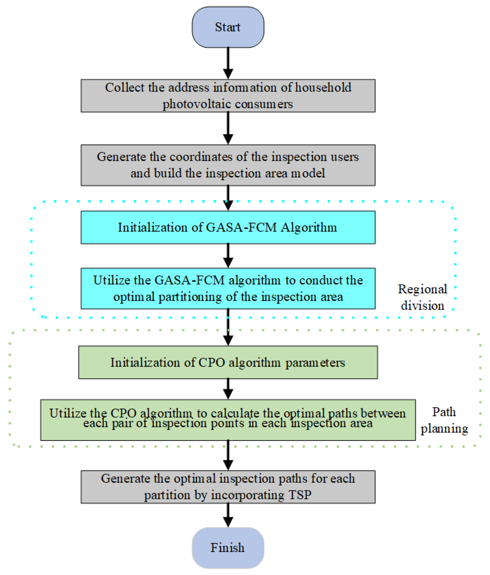
2.1. Overall Process

First, gather the address information of residential PV users to pinpoint and define the target area. Next, generate the coordinates for the inspection users and establish the inspection area model to furnish foundational data for subsequent algorithm implementations.

Upon completing the data gathering and model development, the algorithm initialization phase commences. Specifically, the GASA-FCM algorithm is initialized to establish the initial conditions and parameter configurations for the subsequent regional partitioning. Leveraging this, the GASA-FCM algorithm is employed to optimally partition the inspection area, ensuring a logical division of the target area to streamline subsequent path planning.

Subsequently, the parameters for the CPO algorithm are initialized to furnish the requisite parameter settings for the path planning algorithm. Building on this, the CPO algorithm is deployed to compute the optimal paths between inspection points within each inspection sub-region, ascertaining the most efficient travel routes between inspection points in each sub-region through the application of this algorithm.

Ultimately, the derived optimal paths are integrated into the TSP framework to generate the optimal inspection paths for each sub-region. The comprehensive process flowchart is illustrated in Figure 1.

2.2. Regional Division Model Based on the GASA-FCM Algorithm

To address the issue of dispersed PV users that cannot be easily centralized, this paper proposes a hybrid algorithm combining GASA and FCM, referred to as GASA-FCM. This method integrates the global search capability of the GA and the local search capability of Simulated Annealing (SA) to overcome the tendency of the traditional FCM algorithm to fall into local optima. The GASA-FCM algorithm reduces the dependence on initial clustering centers for household PV users, increases the diversity of classification, and intuitively represents the clustering effect of each data point.

In the GASA-FCM algorithm, regional clustering of household PV users is determined through FCM and optimization using GASA. Specifically, FCM processes the household PV user dataset, determines the minimum objective function, and updates the membership matrix and clustering centers. The clustering principle is as follows:

Fuzzy C-Means Clustering

(1) Determination of the Household PV User Dataset

The FCM algorithm classifies the dataset of household PV users based on the membership degree u of each household. First, the dataset X of household PV users is defined, where each data point represents the PV-related characteristics of a household. The calculation formula is as follows:

$$\mathit{X}=\left[{\mathit{X}}_1,{\mathit{X}}_2,\dots ,{\mathit{X}}_i,\dots ,{\mathit{X}}_n\right]$$

(1)

After determining the household PV dataset, it is necessary to set the constraints on the number of categories to ensure the reasonableness of the clustering, and the calculation formula is shown below:

$$2\le m\le n$$

(2)

After setting the constraint condition for the number of household PV categories, the dataset Y for each category of household PV users is determined, and the calculation formula is as follows:

$$Y=\left[Y_1,Y_2,···,Y_j,···,Y_m\right]$$

(3)

(2) Determination of the Minimum Objective Function for Household PV

After determining the dataset Y for each category of household PV users, the number of cluster centers is selected, and the positions of the cluster centers are initialized randomly. Subsequently, the distance from each data point representing a household PV user to the cluster centers is determined, with the calculation formula as follows:

$$d_{ij}={∥X_i-C_j∥}_2\sqrt{\sum _{l=1}^g{\left(X_{il}-C_{jl}\right)}^2}$$

(4)

In the formula, $d_{ij}$ represents the distance from the i-th data point of a PV user to the j-th cluster center and is the number of feature parameters in Y. After determining the distance from each data point representing a household PV user to the cluster centers, the membership degree of each data point to the household PV category Y needs to be calculated. Specifically, data points closer to the cluster center will have a higher membership degree, while those farther away will have a lower membership degree, with the calculation formula as follows:

$$u_{ij}={\displaystyle \frac{d_{ij}^{-\frac{2}{b-1}}}{{\displaystyle \sum _{l=1}^m}{d}_{ij}^{-\frac{2}{b-1}}}}$$

(5)

where $u_{ij}$ is the membership degree of the i-th data point of a PV user to the j-th cluster, and b is the membership weight factor, which describes the degree to which a PV user belongs to a specific cluster.

After obtaining the expressions for distance and membership degree, the clustering process is further quantified by defining an objective function. The objective function $JB$ is minimized to achieve better clustering performance for household PV users. The calculation formula is as follows:

$$Jb=min\left(\sum _{i=1}^n\sum _{j=1}^m{u}_{ij}^b{d}_{ij}^2\right)$$

(6)

where n is the total number of household PV data points, and c is the number of cluster centers.

(3) Updating the Membership Matrix and Cluster Centers

After calculating the minimum objective function, the membership matrix $C_j$ needs to be updated. The matrix $C_j$ can be calculated using the current membership degrees $u_{ij}$, simultaneously updating the center of clustering for each category to be closer to the center of the distribution of data points for that category with the calculation formula as follows:

$$C_j=\sum _{i=1}^n{\displaystyle \frac{u_{ij}^b}{{\displaystyle \sum _{i=1}^n}{u}_{ij}^b}}$$

(7)

The updated cluster center for each cluster C is represented as follows:

$$C=\left[C_1,C_2,···,C_j,···,C_m\right]$$

(8)

During the update process, the solution to Equation (7) is obtained using the Lagrange method, and the result is as follows:

$$E_q={\displaystyle \frac{{\displaystyle \sum _{j=1}^m}{u}_{ij}^e{X}_j}{{\displaystyle \sum _{j=1}^m}{u}_{ij}^e}}$$

(9)

where e is the weighting exponent, a membership factor that determines the fuzziness between clusters. A larger e value results in less distinct boundaries between clusters.

(4) Objective Function Optimization

After establishing the FCM algorithm model, the clustering of household PV users may fall into local optima instead of achieving global optimality. Therefore, the GASA-FCM algorithm is introduced to leverage the global search capability of the GA and enhance the local search capability of SA. This approach better addresses the issue of local optima in FCM.

First, the fitness function is constructed for assessing the quality of the clustering results and is calculated as follows:

$$g\left(x\right)={\displaystyle \frac{1}{Jb}}$$

(10)

A uniformly distributed random number $\epsilon$ in the interval [0, 1] is generated. If $\epsilon <P$, the new solution is accepted; otherwise, it is rejected. The probability selection function is related to the new and current values of the fitness function as well as the current temperature. In this way, new clustering results can be dynamically accepted or rejected during the optimization process. The probability selection function is calculated as follows:

$$P=\left\{\begin{array}{cc}{e}^{{\displaystyle \frac{g\left(x\right)-g\left(x^{\prime }\right)}{T}}}& g\left(x^{\prime }\right)<g\left(x\right)\\ 1& g\left(x^{\prime }\right)\ge g\left(x\right)\end{array}\right.$$

(11)

where $g\left(x^{\prime }\right)$ is the new value of the fitness function, $g\left(x\right)$ is the current value of the fitness function, and $T_{\phi }$ is the current temperature.

After establishing the fitness and probability selection functions, in order to control the convergence rate of the optimization process, it is necessary to control the temperature reduction, so it is necessary to establish the cooling function, which is calculated as follows:

$$\begin{array}{cc}{T}_{\phi +1}=r{T}_{\phi }& r\in \left(0,1\right)\end{array}$$

(12)

where $g_{max}$ is the initial temperature.

Finally, the algorithm terminates under certain conditions. The maximum number of iterations $g_{max}$ and the minimum temperature $T_{\mathrm{I}}$ are set as constraints to end the loop, When the maximum number of iterations is reached or the temperature is reduced to the lowest temperature, the optimization process ends and the final clustering result is obtained, calculated as follows:

$$\left\{\begin{array}{c}{g}_{\mathrm{en}}>g_{max}\\ T_{\mathrm{c}}<T_{\mathrm{I}}\end{array}\right.$$

(13)

2.3. Clustering Validity Evaluation Metrics

Clustering validity evaluation metrics are standards for measuring the performance of clustering algorithms, used to assess the accuracy and reliability of clustering results. Among these, the silhouette coefficient evaluates clustering effectiveness by combining cohesion and separation. Its value ranges from −1 to 1, with higher values indicating better clustering performance.

Silhouette Coefficient

The silhouette coefficient $s\left(i\right)$ for a PV user point i is calculated as follows:

$$s\left(i\right)={\displaystyle \frac{b\left(i\right)-a\left(i\right)}{max\left\{a\left(i\right)-b\left(i\right)\right\}}}$$

(14)

where $X_i$ represents the cohesion, and b(i) represents the separation. If the silhouette coefficient $s\left(i\right)$ approaches 1, it indicates that point i is very similar to other points within its cluster and dissimilar to points in other clusters, suggesting good clustering performance. If it approaches −1, point i may be incorrectly assigned to its cluster and should be considered for reassignment. If it approaches 0, point i is likely on the boundary between two clusters.

2.4. Path Planning Algorithm Model

After identifying the optimal distribution regions, it is necessary to determine the optimal inspection paths between PV users via an algorithm. The optimal inspection path should minimize inspection time and follow the shortest possible route. The CPO is distinguished by its short computation time, short path length, and a reduced number of path points, which make it suitable for rapidly planning the optimal path between two points. Consequently, the CPO algorithm is employed to ascertain the optimal inspection paths between inspection points.

In the CPO algorithm, the solutions for the optimal inspection paths are updated by simulating the four defensive behaviors of the crested porcupine (CP). These behaviors are categorized into four stages: the first, second, third, and fourth defense stages. The first two stages constitute the exploration phases, whereas the last two stages are the exploitation phases.

2.4.1. Initialization

The initialization process of the CPO algorithm is similar to other algorithms based on meta-heuristic populations. CPO also starts the search process from an initial set of individuals, which are generated according to Equation (15), which contains the number of individuals, lower and upper bounds on the range of the search patrol paths, and a randomly generated vector. The initial population consists of the positions of the individual solutions, represented as a matrix form, where each row represents a solution and each column represents a dimension of the solution.

$$\begin{array}{cc}\overrightarrow{X{X}_i}=\overrightarrow{L}+\overrightarrow{r}\left(\overrightarrow{U}-\overrightarrow{L}\right)& i=1,2,···,N^{\prime }\end{array}$$

(15)

where $N^{\prime }$ represents the number of individuals (population size), $\overrightarrow{X{X}_i}$ is the i-th candidate solution in the search space, $\overrightarrow{L}$ and $\overrightarrow{U}$ are the lower and upper bounds of the inspection path range, respectively, and $\overrightarrow{r}$ is a randomly generated vector between 0 and 1. The initial population is represented as follows:

$$XX=\left[\begin{array}{c}X{X}_1\\ X{X}_2\\ ⋮\\ X{X}_i\\ ⋮\\ X{X}_{N^{\prime }}\end{array}\right]=\left[\begin{array}{cccccc}x{x}_{1,1}& x{x}_{1,2}& \dots & x{x}_{1,j}& \dots & x{x}_{1,d}\\ x{x}_{2,1}& x{x}_{2,2}& \dots & x{x}_{2,j}& \dots & x{x}_{2,d}\\ ⋮& ⋮& ⋮& ⋮& ⋮& ⋮\\ x{x}_{i,1}& x{x}_{i,2}& \dots & x{x}_{i,j}& \dots & x{x}_{i,d}\\ ⋮& ⋮& ⋮& \dots & ⋮& ⋮\\ x{x}_{N^{\prime },1}& x{x}_{N^{\prime },2}& \dots & x{x}_{N^{\prime },j}& \dots & x{x}_{N^{\prime },d}\end{array}\right]$$

(16)

where $x{x}_{i,j}$ denotes the j-th position of the i-th solution, and D represents the dimensionality of the problem.

2.4.2. Cyclic Population Reduction Technique

The cyclic population reduction (CPR) technique is a novel method proposed in the CPO algorithm. This strategy involves periodically removing some individuals from the population to accelerate convergence and then reintroducing them to enhance diversity and avoid local minima, which could prevent finding the optimal inspection path. The process is determined by a cyclic variable T, which specifies the number of times this operation is performed during optimization. The mathematical model for cyclically reducing the population size is as follows:

$$N=N_{min}+\left(N^{\prime }-N_{min}\right)\left(1-\left({\displaystyle \frac{t\%\frac{T_{max}}{T}}{\frac{T_{max}}{T}}}\right)\right)$$

(17)

where T is the variable used to determine the number of cycles, t is the current iteration, $Tmax$ is the maximum number of iterations, % denotes the modulo operator (remainder), and $N_{min}$ is the minimum number of individuals in the newly generated population.

2.4.3. Exploration Phase

(1) First Defense Stage

The algorithm updates the position of an individual based on the optimal inspection path solution for the current iteration number and a randomly generated vector. The random vectors are generated based on a normal distribution and take values between 0 and 1. In this way, the individual can move in a larger range in the search space, increasing the diversity of the search and facilitating the discovery of new potential optimal solutions.

$$\overrightarrow{x{x}_i^{t+1}}=\overrightarrow{x{x}_i^t}+{\tau }_1\left|2{\tau }_2\overrightarrow{x{x}_{CP}^t}-\overrightarrow{y_i^t}\right|$$

(18)

where $\overrightarrow{x{x}_{CP}^t}$ is the optimal inspection path solution at iteration t.$\overrightarrow{y_i^t}$ is the vector generated between the i-th individual and a randomly selected individual from the population at iteration t, ${\tau }_1$ is a random number based on a normal distribution, and ${\tau }_2$ is a random value between 0 and 1. The mathematical formula for generating $\overrightarrow{y_i^t}$ is as follows:

$$\overrightarrow{y_i^t}={\displaystyle \frac{\overrightarrow{x_i^t}+\overrightarrow{x_r^t}}{2}}$$

(19)

where r is a random number between $[1,N]$.

(2) Second Defense Stage

The second defense phase is updated in a way that involves two random integers and a randomly generated binary vector. In this way, the positions of the individuals are adjusted according to other randomly selected individuals, further expanding the search range and enhancing the global search capability of the algorithm. This randomness helps to prevent the algorithm from falling into a local optimum prematurely and improves the probability of finding a globally optimal solution. The updated solution rule is as follows:

$$\overrightarrow{x{x}_i^{t+1}}=\left(1-\overrightarrow{U_1}\right)\overrightarrow{x{x}_i^t}+\overrightarrow{U_1}\left(\overrightarrow{y}+{\tau }_3\left(\overrightarrow{x{x}_{r1}^t}-\overrightarrow{x{x}_{r2}^t}\right)\right)$$

(20)

where $r_1$ and $r_2$ are two random integers between 1 and N, ${\tau }_3$ is a randomly generated number between 0 and 1, and $\overrightarrow{U_1}$ is a binary vector.

2.4.4. Development Phase

(1) Third Defense StageAn individual’s position update is affected by several factors, including the random number, parameters controlling the search direction, defense factors, and odor diffusion factors. Together, these parameters determine the direction and step size of the individual’s movement in the search space. In this way, the algorithm can perform a detailed search in the vicinity of the discovered potential optimal solution and improve the accuracy of the solution. Among them, the formulas for the defense factor and odor diffusion factor take into account the value of the individual’s objective function, the number of iterations, and the randomly generated vectors, enabling the algorithm to dynamically adjust the search strategy according to the current search state. The updated solution rule is as follows:

$$\overrightarrow{x{x}_i^{t+1}}=\left(1-\overrightarrow{U_1}\right)\times \overrightarrow{x{x}_i^t}+\overrightarrow{U_1}\times \left(\overrightarrow{x{x}_i^t}+S_i^t\times \left(\overrightarrow{x{x}_{r2}^t}-\overrightarrow{x{x}_{r3}^t}\right)-{\tau }_3\times \overrightarrow{\delta }\times {\gamma }_t\times S_i^t\right)$$

(21)

where $r_3$ is a random number within [1,N], $\delta$ is a parameter controlling the search direction defined by Equation (22), $\overrightarrow{x{x}_i^t}$ is the position of the i-th individual at the t-th iteration, ${\gamma }_t$ is the defense factor defined by Equation (23), ${\tau }_3$ is a random value within the interval [0, 1], and $S_i^t$ is the odor diffusion factor defined by Equation (24).

$$\overrightarrow{\delta }=\left\{\begin{array}{cc}1& \overrightarrow{rand}\le 0.5\\ -1& \overrightarrow{rand}>0.5\end{array}\right.$$

(22)

$${\gamma }_t=2\times rand\times {\left(1-{\displaystyle \frac{t}{t_{max}}}\right)}^{{\displaystyle \frac{t}{t_{max}}}}$$

(23)

$$S_t^i=exp\left({\displaystyle \frac{f\left(x_t^i\right)}{{\displaystyle \sum _{k=1}^N}f\left(x_t^k\right)+\epsilon }}\right)$$

(24)

In these formulas, $f\left(x_t^i\right)$ represents the objective function value of the i-th individual at the t-th iteration. The term $\epsilon$ is a very small value to avoid division by zero. $\overrightarrow{rand}$ is a randomly generated vector between 0 and 1, while $\overrightarrow{rand}$ is also a randomly generated variable between 0 and 1. N denotes the population size, t is the current iteration, and $t_{max}$ is the maximum number of iterations.

(2) Fourth Defense Stage

The updating approach involves variables that determine the speed of convergence, random values, and parameters that affect the average strength of the predator. Together, these factors determine the convergence speed and stability of an individual during the search process. In this way, the algorithm can ensure the convergence speed while avoiding premature convergence to a local optimal solution. Among them, the updating formulas for parameters such as the mass, objective function value, and speed of the individual take into account randomly generated vectors and variables, which enables the algorithm to dynamically adjust the state of the individual during the search process to improve the search efficiency and quality of the solution. The updated solution rule is as follows:

$$\overrightarrow{x{x}_i^{t+1}}=\overrightarrow{x{x}_{CP}^t}+\left(\alpha \left(1-{\tau }_4\right)+{\tau }_4\right)\left(\delta \overrightarrow{x{x}_{CP}^t}-\overrightarrow{x{x}_i^t}\right)-{\tau }_5\delta {\gamma }_t\overrightarrow{F_i^t}$$

(25)

where $\alpha$ is a variable that determines the convergence rate, ${\tau }_4$ and ${\tau }_5$ are random values in the interval [0, 1], and $\overrightarrow{F_i^t}$ is the average force affecting the i-th predator’s CP, provided by the inelastic collision law and defined by Equation (26).

$$\overrightarrow{F_i^t}=\overrightarrow{{\tau }_6}{m}_i\left(\overrightarrow{v_i^{t+1}}-\overrightarrow{v_i^t}\right)$$

(26)

$$m_i={\displaystyle \frac{f\left(\overrightarrow{x_i^k}\right)}{e^{{\displaystyle \sum _{k=1}^N}f\left(\overrightarrow{x_k^t}\right)+\epsilon }}}$$

(27)

$$\overrightarrow{v_i^t}=\overrightarrow{x_i^t}$$

(28)

$$\overrightarrow{v_i^{t+1}}=\overrightarrow{x{x}_r^t}$$

(29)

In these formulas, $m_i$ denotes the mass of the i-th individual at iteration t,$f\left(·\right)$ represents the objective function, $\overrightarrow{v_i^{t+1}}$ is the final velocity of the i-th individual at iteration t + 1, $\overrightarrow{v_i^t}$ is the initial velocity of the i-th individual at iteration t, and ${\tau }_6$ is a randomly generated vector between 0 and 1.

3. Simulation Results and Analysis

The simulation experiments include clustering analysis experiments and path planning experiments. The laboratory platform configuration is as follows: Intel i7-11800H processor(Intel Corporation, Santa Clara, California, USA), 16 GB of memory(Samsung, Seoul, Republic of Korea), Windows 11 operating system, and MATLAB 2022a as the simulation software.

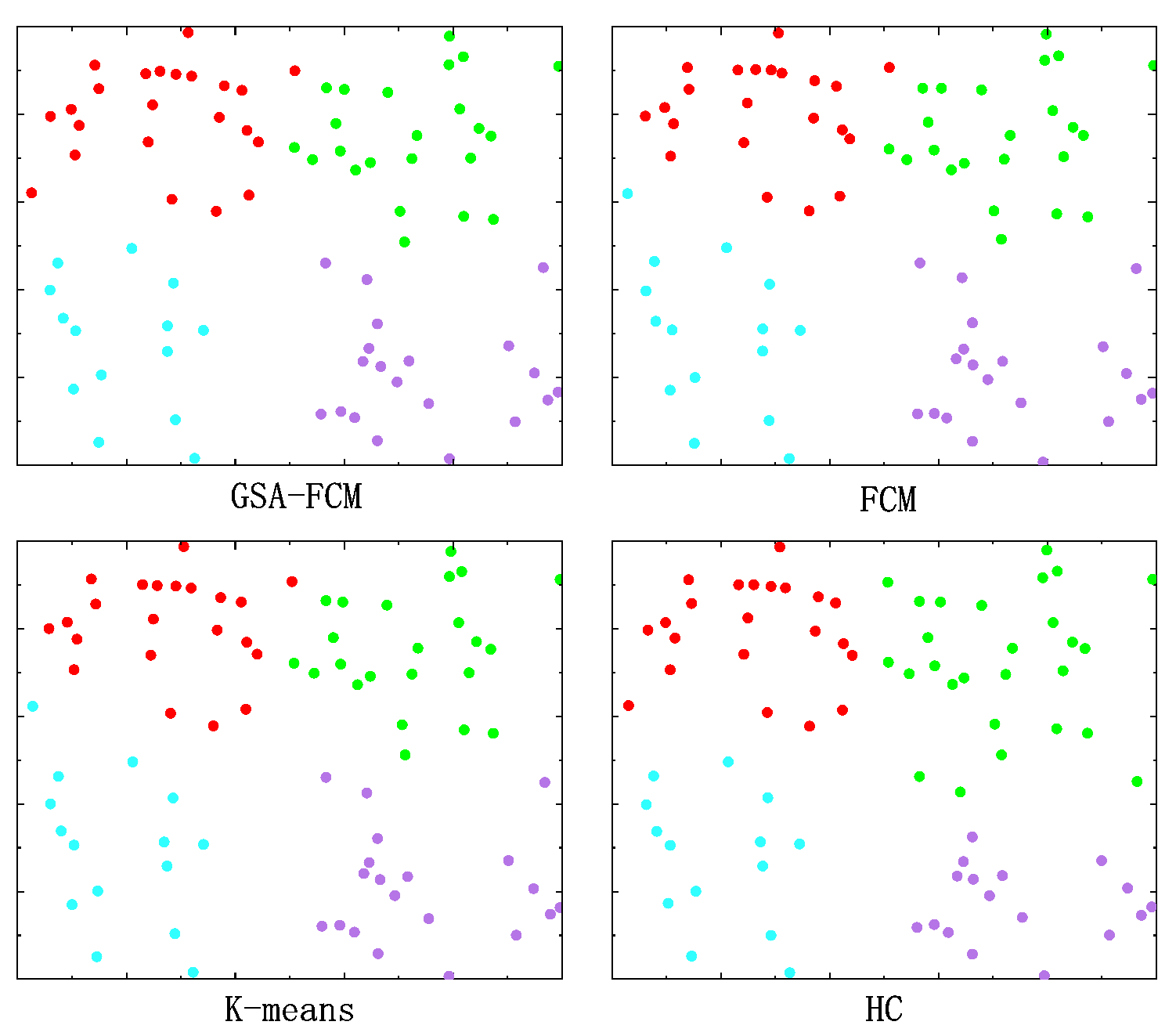
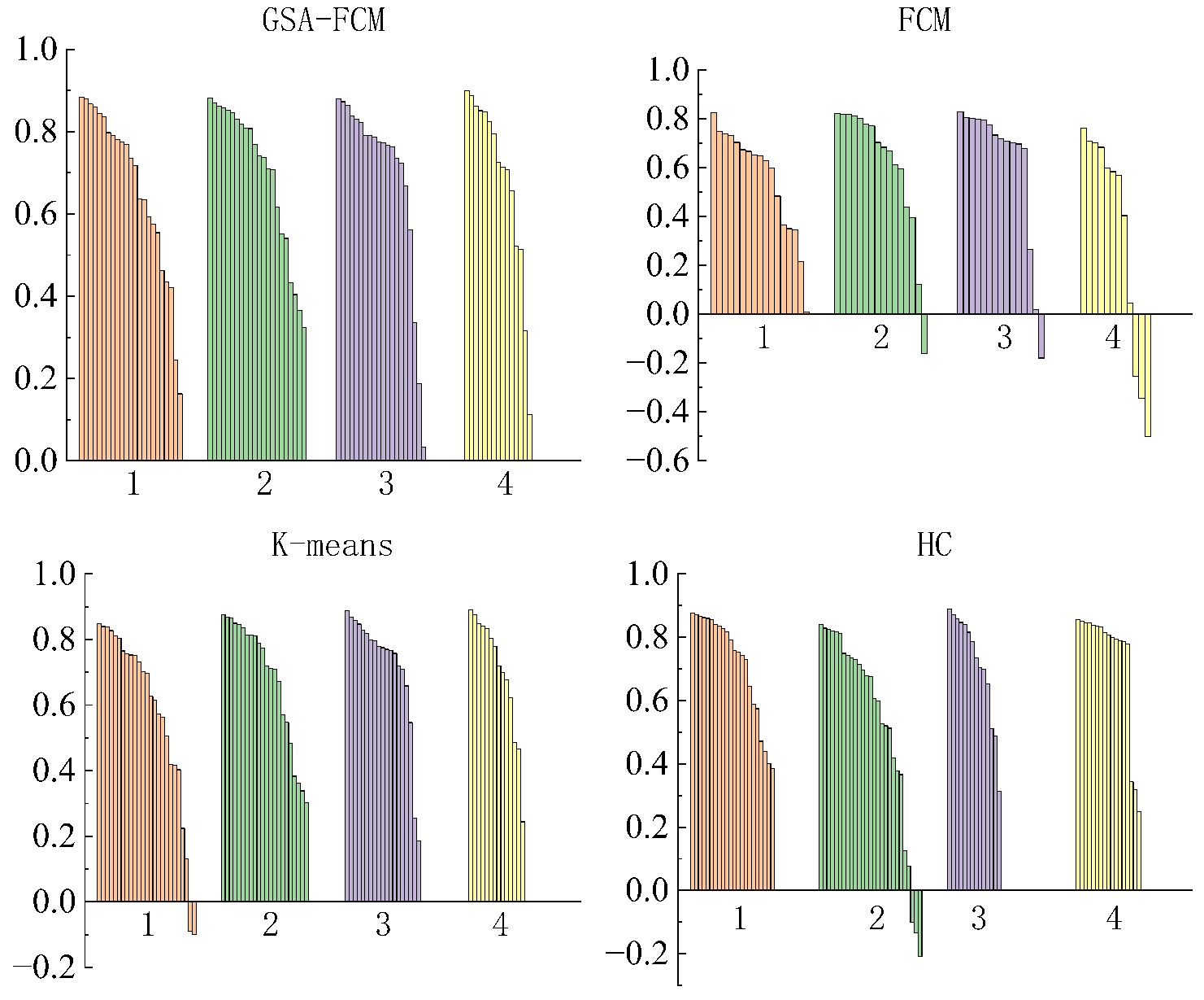
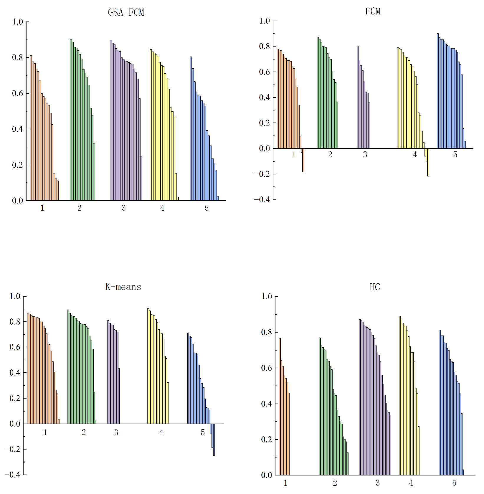
3.1. Clustering Algorithm Simulation Experiments

In all the experiments conducted in this section, the clustering quality is evaluated using the metric defined in Equation (14). The GASA-FCM algorithm proposed in this paper is compared with the FCM algorithm, K-means algorithm, and HC algorithm.

To obtain meaningful results, the data used in this section are all sourced from real datasets obtained through field surveys.

Table 1. Data sources.

Dataset	Number of Data Points	Data	Feature Type
BLERSSI	6611	6	Integer

lists the datasets used in the experiments, which are primarily sourced from the UCI Machine Learning Repository.

First, the clustering results of the four algorithms are visually obtained using MATLAB. For ease of verification, the number of cluster centers is set to four, and the total number of samples is 80. The figures from left to right represent the clustering results of GASA-FCM, FCM, K-means, and HC, respectively.

Comparison of Average Silhouette Values of Four Clustering Algorithms

Figure 2 shows a comparison of the results of the four clustering algorithms, and the dots of the same color represent the same clustering area.Figure 3 and Figure 4 illustrate the average silhouette values of the four algorithms when the number of clusters is set to four and five, respectively. In this subsection, the average silhouette value is employed to assess the clustering performance. When the number of clusters is four, the average silhouette values of GASA-FCM, FCM, K-means, and HC are 0.682671, 0.61261, 0.659822, and 0.6717, respectively. The average silhouette value of GASA-FCM is 11.43% higher than that of FCM, 3.5% higher than that of K-means, and 1.3% higher than that of HC. When the number of clusters is five, the average silhouette value of GASA-FCM is 7.5% higher than that of FCM, 1.1% higher than that of K-means, and 2.6% higher than that of HC.

Table 2. Comparison of average silhouette values of four algorithms.

Number of Clusters	GASA-FCM	FCM	k-Means	HC
4	0.682671	0.61261	0.659822	0.6717
5	0.621103	0.577799	0.614267	0.605279

clearly demonstrates that the average silhouette value of the GASA-FCM algorithm remains the highest among the four algorithms. This is attributed to the fact that the GASA-FCM algorithm optimizes the initial cluster centers by integrating GA and SA. The optimized cluster centers are subsequently assigned to FCM, thereby circumventing the randomness of the initial values. During the execution of the algorithm, the cluster centers are continuously updated, leading to more stable and accurate clustering results and consequently higher average silhouette values.

3.2. Path Planning Simulation Experiments

To validate the superiority of the CPO algorithm in identifying the optimal path within a static environment, this paper conducts a comparison between the CPO algorithm and other algorithms through computer-based simulation experiments.

In the simulation environment, the SSA, PSO, GWO, and CPO algorithms are employed for path planning on 20 × 20 and 40 × 40 grid maps. Each algorithm is executed independently 20 times. The average path length, average number of path points, average runtime, the shortest path among the 20 runs, and the path standard deviation are compared to assess the performance.In

Table 3. Algorithm comparison scenarios.

Scenario	Simulation Environment	SSA	PSO	GWO	CPO
1.1	20 × 20	√
1.2	20 × 20		√
1.3	20 × 20			√
1.4	20 × 20				√
2.1	40 × 40	√
2.2	40 × 40		√
2.3	40 × 40			√
2.4	40 × 40				√

, we conducted a series of algorithm comparison scenarios under different simulation environments. The performance of SSA, PSO, GWO, and CPO algorithms was evaluated in various settings, including different grid sizes of the simulation environment.

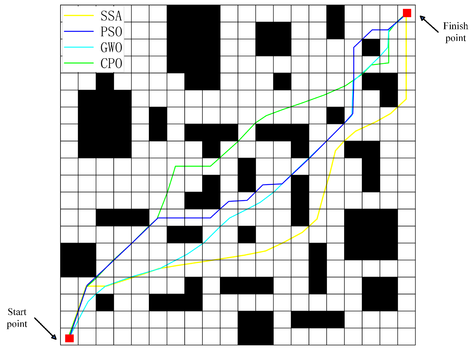
3.2.1. The 20 × 20 Simulation Environment

To thoroughly investigate the path planning performance of the CPO algorithm in small-scale environments, we first conducted simulation experiments on a 20 × 20 grid map. By comparing the CPO algorithm with several other mainstream path planning algorithms (such as the SSA, PSO, and GWO) under the same environmental conditions, we aimed to preliminarily evaluate the advantages of the CPO algorithm in terms of solution efficiency, path length, and stability. The following section will present and analyze the results of this simulation experiment in detail.

The comparative data derived from the simulation experiments are presented in

Table 4. Comparison of simulation results for 20 × 20 grid.

Scenario	Algorithm	Average Path Length	Average Path Points	Average Runtime (s)	Shortest Path	Path Standard Deviation
1.1	SSA	30.08012	16.95	2.968242	28.605	0.92838
1.2	PSO	29.63031	17.85	1.889432	27.5668	1.118081
1.3	GWO	29.49351	16.6	1.301083	27.9007	0.714452
1.4	CPO	29.22382	16.5	1.163811	28.4865	0.372128

, and the 20 × 20 random grid simulation map is depicted in Figure 5. As indicated in Table 4, the CPO algorithm attains near-optimal average path length and a minimal number of path points, demonstrating its capability in planning shorter paths with fewer path points. The average runtime of the CPO algorithm is merely 1.16 s, which is significantly shorter than the SSA’s 2.97 s and PSO’s 1.89 s, and also shorter than the GWO’s 1.30 s. This illustrates that the CPO algorithm holds a substantial advantage in terms of solving efficiency, enabling it to rapidly identify near-optimal solutions. The path standard deviation of the CPO algorithm is only 0.37, which is considerably lower than that of the other algorithms, indicating a high level of stability across multiple runs. Overall, the CPO algorithm exhibits marginally superior performance compared to the other three algorithms in terms of average path length and runtime. Although it only marginally surpasses the SSA regarding shortest path length, it significantly outperforms the other algorithms in terms of path standard deviation. This suggests that the CPO algorithm possesses high computational efficiency and stability in simple maps with optimal path lengths. In conclusion, within the 20 × 20 grid map, the CPO algorithm demonstrates favorable performance in path length, runtime, and stability, thereby proving its superiority in path planning within small-scale environments.

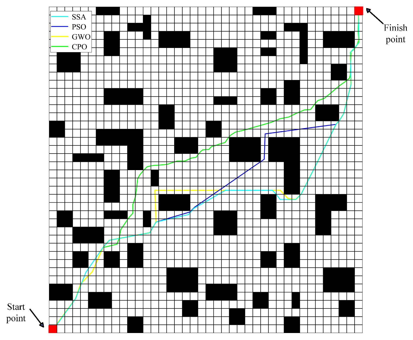
3.2.2. The 40 × 40 Simulation Environment

To further validate the path planning capability of the CPO algorithm in more complex and larger-scale environments, we subsequently conducted simulation experiments on a 40 × 40 grid map. By comparing and analyzing the performance of the CPO algorithm with other algorithms, such as the SSA, PSO, and GWO, under the same complex environmental conditions, we aim to comprehensively assess the effectiveness and stability of the CPO algorithm when addressing large-scale, high-complexity path planning problems. The following section will present and analyze in detail the specific results of this simulation experiment.

The comparative data obtained from the simulation experiments are presented in

Table 5. Comparison of simulation results for 40 × 40 grid.

Scenario	Algorithm	Average Path Length	Average Path Points	Average Runtime (s)	Shortest Path	Path Standard Deviation
2.1	SSA	62.19886	22.6	12.94032	58.6576	2.440526
2.2	PSO	63.21584	22.3	7.37224	57.0243	4.447651
2.3	GWO	62.59868	21.05	7.378058	59.0857	2.285714
2.4	CPO	61.15182	21.65	5.879644	58.9176	0.953437

, and the 40 × 40 random grid simulation map is depicted in Figure 6. As indicated by Table 5, the CPO algorithm exhibits favorable performance in terms of average path length, with a value of only 61.15, representing a reduction compared to the other algorithms. This implies that, even in a more complex environment, the CPO algorithm is still capable of planning shorter paths. Furthermore, the average number of path points is relatively small, which further substantiates its effectiveness. The average runtime of the CPO algorithm is 5.88 s, which is significantly shorter than the SSA’s 12.94 s, PSO’s 7.37 s, and the GWO’s 7.38 s. This demonstrates that, in a larger-scale environment, the CPO algorithm still maintains a high level of solving efficiency and can rapidly identify near-optimal solutions. Although the path standard deviation of the CPO algorithm has increased on the 40 × 40 grid map, it remains at a low value (0.95), indicating good stability. This means that the CPO algorithm can still sustain consistent performance in more complex environments.

In summary, on the 40 × 40 grid map, the CPO algorithm also demonstrates favorable performance in terms of path length, runtime, and stability, thereby verifying its superiority in path planning within larger-scale environments.

Considering the simulation results of both the 20 × 20 and 40 × 40 grid maps, the CPO algorithm demonstrates excellent path planning performance across different scales. Whether in the smaller 20 × 20 grid map or the larger 40 × 40 grid map, the CPO algorithm consistently maintains shorter path lengths, faster solving speeds, and higher stability. This indicates that the CPO algorithm has good versatility across different scales. Compared with other algorithms (the SSA, PSO, and the GWO), the CPO algorithm shows significant advantages in path length, runtime, and stability, especially in solving efficiency and stability.

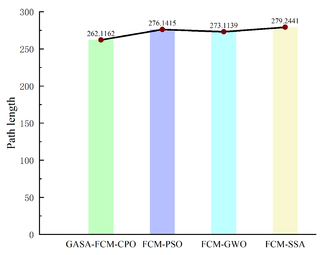
3.3. Comprehensive Simulation Experiments

To assess the effectiveness of the proposed method in addressing the MTSP, this paper randomly generates 28 inspection points on a 40 × 40 random grid map. It then compares the proposed algorithm with the FCM-PSO, FCM-GWO, and FCM-SSA algorithms to validate its effectiveness. Figure 7 illustrates the comparison of the four algorithms in solving the multi-start multi-traveler problem with four travelers on the map. As depicted in the figure, the proposed algorithm yields shorter path lengths compared to the other three algorithms. Figure 8 displays the solution results of the MTSP problem obtained using the proposed algorithm on the map.

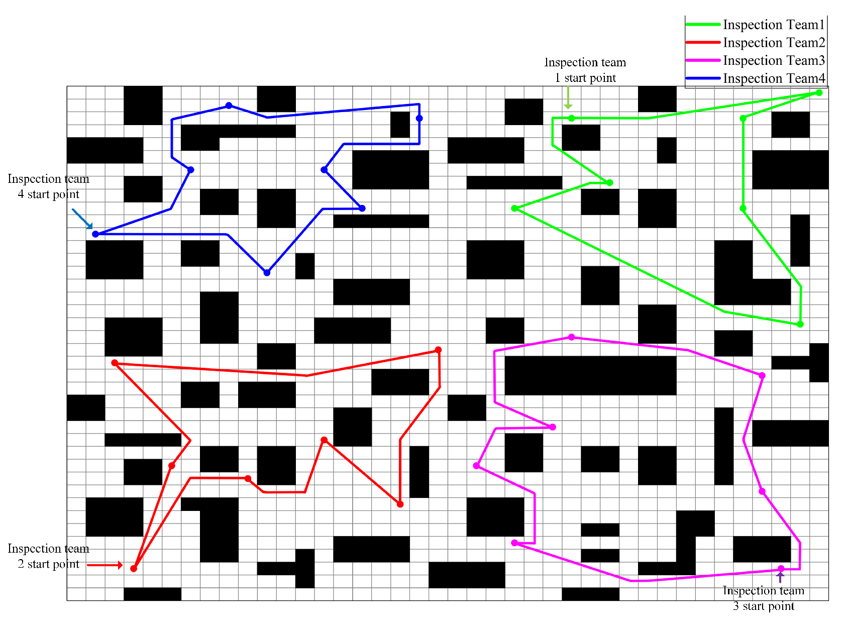
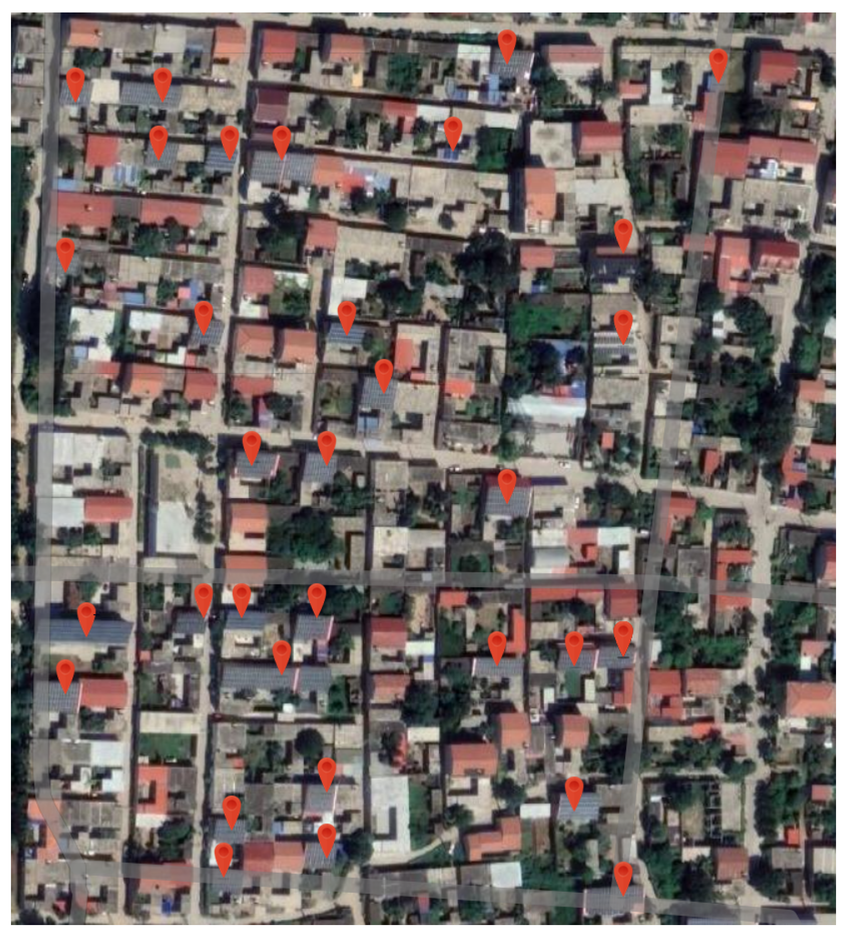
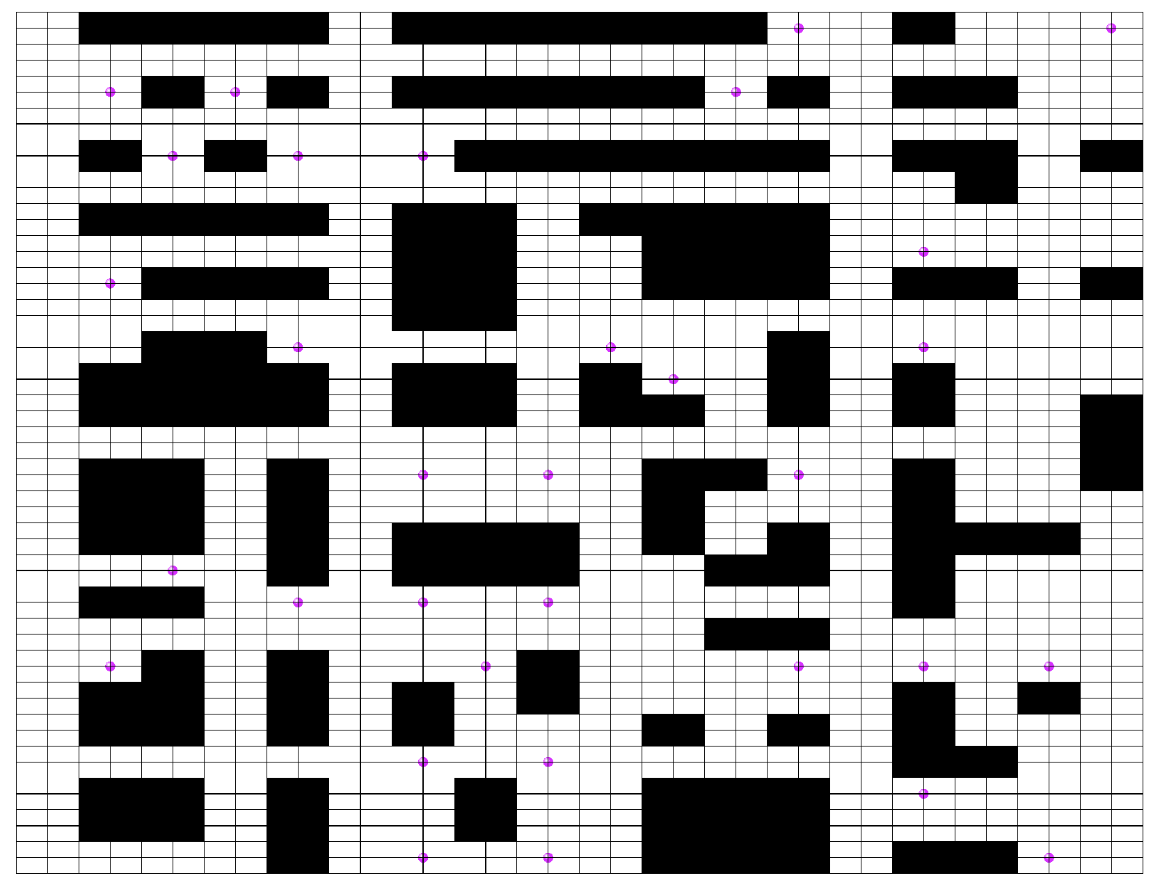
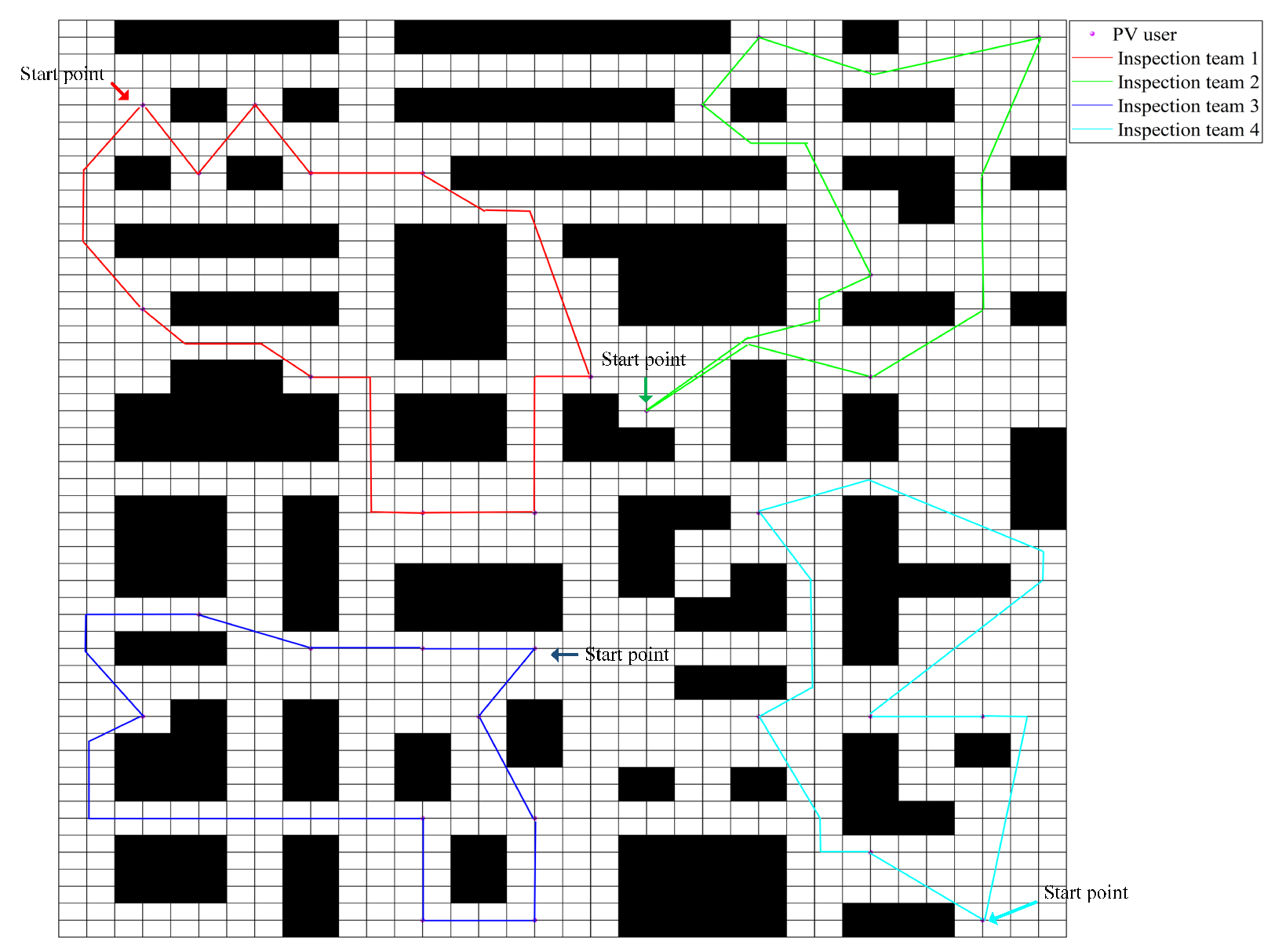
3.4. Practical Case Study

In order to verify the effectiveness of the rural multi-area PV inspection path planning method based on the CPO algorithm proposed in this paper in practical applications, in this study, 32 distributed PV power stations within the county area of West Two Rivers Village, Zhang Duangu Town, Wuji County, Hebei Province, are selected as research objects. These power stations are distributed in rural areas, the geographic location data are obtained by the BeiDou positioning system, and the geographic grid is constructed by combining with the DEM elevation model, which provides data support for path planning.

Based on the BeiDou Navigation Satellite System (BDS) positioning data of the 32 distributed PV sites in the county area of West Two Rivers Village, Zhang Duangu Town, Wuji County, Hebei Province, as shown in Figure 9, the corresponding grid map is obtained through analog conversion, as shown in Figure 10. In the grid map, the white areas represent the roads, the black areas represent the obstacles, and the purple points represent the locations of the PV equipment requiring inspection. Subsequently, the path planning method based on the CPO algorithm is used for inspection path planning, as shown in Figure 11, where the lines of different colors represent the inspection paths of the four inspection teams, and the purple point represents the location of the PV user (PV equipment that needs to be inspected).

From Figure 11, the CPO algorithm successfully plans inspection paths for multiple inspection teams, which are able to cover all the PV devices, and the algorithm takes into account the obstacle constraints in the grid map during the planning process by introducing the obstacle avoidance distance mechanism. Compared with the traditional manual inspection, the total mileage is shortened by 38.7%, from 217.4 km to 133.2 km, and the path smoothness is improved by 52.3%, which verifies the engineering applicability of the method in complex rural terrain. In addition, the CPO algorithm shows a high degree of stability and adaptability in real scenarios and is able to quickly find the optimal or near-optimal inspection paths, demonstrating advantages in terms of path length, running time, and stability.

4. Conclusions

The PV inspection planning problem has a strong practical application background and theoretical research value. It is also a pressing pain point and challenge that needs to be addressed in the operation and maintenance of rural PV systems at present.

This paper proposes a rural multi-region PV inspection path planning method based on the CPO algorithm, which combines clustering techniques with path planning algorithms to solve the MTSP. Firstly, the GASA-FCM algorithm is used for region division, and its superior clustering performance compared to other algorithms is verified through the silhouette coefficient metric. After division, considering the actual situation in rural areas, the obstacle-avoidance distance between two points is used to replace the traditional Euclidean distance.

The experimental results show that the CPO algorithm outperforms other algorithms (such as the SSA, PSO, and GWO) in calculating obstacle-avoidance paths, exhibiting the characteristics of shorter path lengths, stronger stability, and higher adaptability. Finally, through comprehensive simulation experiments and real-world case studies, the feasibility of the proposed algorithm in solving the MTSP is verified.

References

1. Tong, L.; Geng, Y.; Zhang, Y.; Zhang, Y.; Wang, H. Testing the effectiveness of deploying distributed photovoltaic power systems in residential buildings: Evidence from rural China. Environ. Impact Assess. Rev. 2024, 104, 107300. [Google Scholar] [CrossRef]
2. Zhu, T.; Chang, X.; Zhu, F.; Shen, Y.; Zhu, L.; Xu, C. Empirical study on sustainable energy development goals: Analysis of rural roof distributed photovoltaic systems in Jiangsu, China. Phys. Chem. Earth 2024, 136, 103711–103720. [Google Scholar] [CrossRef]
3. Su, X.; Liu, P.; Mei, Y.; Chen, J. The role of rural cooperatives in the development of rural household photovoltaics: An evolutionary game study. Energy Econ. 2023, 126, 106962. [Google Scholar] [CrossRef]
4. Li, W.; Zou, Y.; Yang, H.; Fu, X.; Li, Z. Two stage stochastic Energy scheduling for multi energy rural microgrids with irrigation systems and biomass fermentation. Energy Econ. 2025, 16, 1075–1087. [Google Scholar] [CrossRef]
5. Cheikhrouhou, O.; Khoufi, I. A comprehensive survey on the Multiple Traveling Salesman Problem: Applications, approaches and taxonomy. Comput. Sci. Rev. 2021, 4, 100369–100380. [Google Scholar] [CrossRef]
6. Li, X.; Chen, Y.; Chen, Z.; Huang, Z. Coverage path planning of bridge inspection with Unmanned aerial vehicle. Eng. Appl. Artif. Intell. 2025, 156, 111253. [Google Scholar] [CrossRef]
7. Thongpiem, J.; Punkong, N.; Ratanavilisagul, C.; Kosolsombat, S. Hybrid Genetic Algorithm and Ant Colony Algorithm for Solving Travelling Salesman Problem. In Proceedings of the 2024 IEEE 9th International Conference on Computational Intelligence and Applications (ICCIA), Haikou, China, 9–11 August 2024. [Google Scholar]
8. Daoqing, Z.; Mingyan, J. Parallel discrete lion swarm optimization algorithm for solving traveling salesman problem. J. Syst. Eng. Electron. 2020, 31, 751–760. [Google Scholar] [CrossRef]
9. Wu, C.; Fu, S.; Pei, J.; Dong, Z. A novel sparrow search algorithm for the traveling salesman problem. IEEE Access 2021, 9, 153456–153471. [Google Scholar] [CrossRef]
10. Tao, Q.; Zhang, T.; Han, J. An approximate parallel annealing Ising machine for solving traveling salesman problems. IEEE Embed. Syst. Lett. 2023, 15, 226–229. [Google Scholar] [CrossRef]
11. Liu, M.; Li, Y.; Li, A.; Huo, Q.; Zhang, N.; Qu, N.; Zhu, M.; Chen, L. A slime mold-ant colony fusion algorithm for solving traveling salesman problem. IEEE Access 2020, 8, 202508–202521. [Google Scholar] [CrossRef]
12. Kerschke, P.; Kotthoff, L.; Bossek, J.; Hoos, H.H.; Trautmann, H. Leveraging TSP solver complementarity through machine learning. Evol. Comput. 2018, 26, 597–620. [Google Scholar] [CrossRef] [PubMed]
13. Arslan, H.; Manguoglu, M. A parallel bio-inspired shortest path algorithm. Computing 2019, 101, 969–988. [Google Scholar] [CrossRef]
14. Nand, R.; Chaudhary, K.; Sharma, B. Single depot multiple travelling salesman problem solved with preference-based step ahead firefly algorithm. IEEE Access 2024, 12, 26655–26666. [Google Scholar] [CrossRef]
15. Zheng, J.; Hong, Y.; Xu, W.; Li, W.; Chen, Y. An effective iterated two-stage heuristic algorithm for the multiple Traveling Salesmen Problem. Comput. Oper. Res. 2022, 143, 105772. [Google Scholar] [CrossRef]
16. Tong, M.; Peng, Z.; Wang, Q. A hybrid artificial bee colony algorithm with high robustness for the multiple traveling salesman problem with multiple depots. Expert Syst. Appl. 2025, 260, 125446. [Google Scholar] [CrossRef]
17. Hamza, A.; Darwish, A.H.; Rihawi, O. A new local search for the bees algorithm to optimize multiple traveling salesman problem. Intell. Syst. Appl. 2023, 18, 200242. [Google Scholar] [CrossRef]
18. Cunha, C.B.; Massarotto, D.F.; Fornazza, S.L.; Mendes, A.B. An ALNS metaheuristic for the family multiple traveling salesman problem. Comput. Oper. Res. 2024, 169, 106750. [Google Scholar] [CrossRef]
19. Tong, S.; Qu, H.; Xue, J. K-DSA for the multiple traveling salesman problem. J. Syst. Eng. Electron. 2023, 34, 1614–1625. [Google Scholar] [CrossRef]
20. Sanyal, S.; Roy, K. Neuro-ising: Accelerating large-scale traveling salesman problems via graph neural network guided localized ising solvers. IEEE Trans. Comput. Aided Des. Integr. Circuits Syst. 2022, 41, 5408–5420. [Google Scholar] [CrossRef]
21. Yang, Z.; Nai, W.; Li, D.; Liu, L.; Chen, Z. A Mixed Generative Adversarial Imitation Learning Based Vehicle Path Planning Algorithm. IEEE Access 2024, in press. [CrossRef]
Figure 1. Overall process flowchart.
Energies 18 02909 g001
Figure 2. Clustering results of four algorithms.
Energies 18 02909 g002
Figure 3. Comparison of household PV inspection areas divided into 4 clusters.
Energies 18 02909 g003
Figure 4. Comparison of household PV inspection areas divided into 5 clusters.
Energies 18 02909 g004
Figure 5. Simulation results of 20 × 20 random grid.
Energies 18 02909 g005
Figure 6. Simulation results of 40 × 40 random grid.
Energies 18 02909 g006
Figure 7. Comparison of the proposed algorithm with other algorithms.
Energies 18 02909 g007
Figure 8. Solution results of the proposed algorithm.
Energies 18 02909 g008
Figure 9. BeiDou positioning data map.
Energies 18 02909 g009
Figure 10. Simulation grid diagram.
Energies 18 02909 g010
Figure 11. Inspection route map.
Energies 18 02909 g011