Generalized Predictive Control of Doubly Fed Variable-Speed Pumped Storage Unit

Abstract

With the increasing penetration of renewable energy, doubly-fed variable speed pumped storage units (DFVSPSUs) are playing an increasingly critical role in grid frequency regulation. However, traditional PI control struggles to address the control challenges posed by the strong nonlinearity of the units and abrupt operational condition changes. This paper proposes an improved β-incremental generalized predictive controller (β-GPC), which achieves precise rotor-side current control through instantaneous linearization combined with parameter identification featuring a forgetting factor. Simulation results demonstrate that under different power command step changes, the traditional PI controller requires up to approximately 0.48 s to reach a steady state while exhibiting a certain degree of oscillations. In contrast, the enhanced β-GPC controller can stabilize the unit in just 0.2 s without any overshoot or subsequent oscillations. It is evident that the proposed controller delivers a superior regulation performance, characterized by a shorter settling time, reduced overshoot, and minimized oscillations.

1. Introduction

The integration of vast amounts of new energy into existing power grids highlights the critical role of doubly fed variable-speed pumped storage units (DFVSPSUs). As an effective means of absorbing this new energy, DFVSPSUs are crucial in the context of a highly penetrative new power grid. A DFVSPSU exhibits a significant adjustable capacity and favorable economic benefits. However, it faces several challenges—most notably, rapid variations in multiple operating conditions that substantially increase control system complexity compared to conventional hydroelectric units. Within the new power system, variable-speed pumped storage units perform critical tasks, such as peak regulation, frequency regulation, and emergency backup. The variable speed pumping and storage unit has the ability to quickly respond to the demand of the power grid, and can always maintain the optimal speed at any head and load, and maintain the optimal efficiency, which plays an important role in the stable operation of the power system. Kougias emphasized the potential of variable speed units in enhancing system flexibility and reliability [1]; Iliev conducted a systematic analysis of variable speed operation of Francis turbines [2]; Valavi demonstrated the critical role of variable speed units in power system frequency regulation and stability [3]. Therefore, the high reliability of DFVSPSUs is essential for ensuring the secure and stable operation of modern power systems.

From a technical perspective, the machine-side converter of the DFVSPSU utilizes stator flux-oriented vector control, while the grid-side converter applies voltage oriented vector control. In the doubly fed induction generator (DFIG) control system, the stator is directly connected to the power grid. Meanwhile, the rotor is connected to the grid via a bidirectional converter, which, in turn, controls the stator of the DFIG to provide both active and reactive power to the grid. The strong coupling and nonlinearity found within the DFIG control system are a significant hurdle. Therefore, conventional proportional integral (PI) controllers exhibit limitations during operational condition transitions. For instance, in doubly-fed induction generator (DFIG) systems, PI controllers demonstrate prolonged settling times [4]; in wind power applications, they show significant overshoot issues [5]; and when dealing with nonlinear dynamic characteristics, PI controllers present notable deficiencies, particularly under rapid load variation conditions, where their regulation performance deteriorates markedly due to time-varying system parameters [6]. Such behaviors fall short of a fast response and high-penetration operational requirements of the pumped storage unit within new high-permeability grids. Furthermore, existing solutions fail to address the adaptation problem between time-variation and linear control laws [7]. Therefore, there is a pressing need to explore more advanced control strategies for the DFVSPSU.

In recent years, various advanced control methods have been incorporated into the control systems of water turbines and pumped storage units. For example, the adaptive fuzzy PID control, fractional-order PID control and hybrid algorithm optimization, sliding mode control and trajectory tracking, neural network and predictive control combination, and nonlinear generalized predictive control methods have been incorporated [8,9,10,11,12]. Fang and Chen showed that as a hydraulic turbine is a nonlinear and time-varying minimum phase system, although the PID governor is simple to control, there are many problems, such as a large overshoot, long adjustment time, and a large error index. At the same time, the PID controller is more dependent on the unit operating conditions, and when the unit is faced with a wide range of operating conditions, it is difficult to determine the parameters to meet the needs of the unit [13]. Because the PID controller is mainly determined by the past and present operation of the unit, it cannot predict the operation of the unit at the next moment. In view of this shortcoming, many advanced control algorithms have been introduced into the hydraulic turbine governor, such as fuzzy PID control; fractional order PID control; sliding mode control; adaptive control; and generalized predictive control. Zhou applied the advanced fuzzy PID control to the hydraulic turbine and realized the online adjustment of the controller parameters, so as to achieve the purpose of optimizing the control effect [14]. Xiong and Shi proposed a fractional order PID (FOPID) double objective function control system using the mixed algorithm (BP-FOA). Simulation and case analysis show that the hydraulic turbine governor optimized by the mixed algorithm has certain improvements in its regulation performance and robustness [15]. Fu and Zhang designed a dynamic sliding mode controller for a hydraulic turbine regulation system based on the sliding mode control method, and then optimized the designed controller parameters by particle swarm optimization and the Gray Wolf hybrid optimization algorithm (PSOGWO). The simulation results show that the designed dynamic sliding mode controller not only improves the control performance of the turbine regulation system and reduces the convergence time of trajectory tracking, but it also significantly reduces the buffeting effect of the sliding mode control and the error of trajectory tracking [16]. Nidhal Ben Khedher proposed a fuzzy logic-based statistical quality control method that integrates fuzzy linguistic variables into control charts to develop a comprehensive fuzzy process efficiency index evaluating mean, target value, and variance. When applied to water meter production in Ha’il, Saudi Arabia, the method (efficiency index < 1) demonstrated more accurate identification of suboptimal production conditions compared to traditional approaches, and was further benchmarked against machine learning techniques [17]. Fathi Troudi Five photovoltaic system MPPT control methods were compared, as follows: the perturbation observation method (PO), the conductance increment method (INC), the artificial neural network method (ANN), the neural network method based on open circuit voltage (FVCO), and the neural network method based on a short circuit current (FCC) to optimize the maximum power output under different environmental conditions [18]. This paper mainly studies the problem of generalized predictive control. Chen and Zhou proposed a new power grid load prediction method based on a BP artificial neural network to improve generalized predictive control. The combined prediction model effectively combines the advantages of the two algorithms and makes up for the shortcomings of generalized prediction in nonlinear system control [19]. Xiao and Liu combined generalized predictive control and signal compensation to propose a nonlinear generalized predictive control method driven by compensation signals. The proposed method loosens the previous condition that the unknown nonlinear term is globally bounded to the Lipschitz condition, and it proves the stability and convergence of the closed-loop system [20]. Song and Ran proposed a frequency control strategy for the hydro turbine system based on generalized predictive control (GPC), on the basis of automatic generation control. The simulation results show that GPC applied to the hydro turbine regulation system can achieve a good output response, effectively solving the frequency regulation problem of the power system, and enhancing the robustness of the system [21]. Chen and Liu designed the double models, a real-time feedback linearization module, and a nonlinear characteristic compensator; proposed a generalized predictive control strategy combining these modules (GPC-DM-RFLM-NCC); and built the HTRS simulation platform, which consists of GPC, double models, a real-time feedback linearization module, and a nonlinear characteristic compensator. The applicability, reliability, and excellent robustness of the proposed GPC-DM-RFLM-NCC are verified by the real data of a hydropower station [22]. The growing prominence of doubly-fed variable-speed pumped storage units (DFVSPSUs) in modern power systems necessitates the development of advanced control strategies to ensure stable operation. However, current research faces several critical challenges, which are as follows: (1) predictive control applications in DFVSPSUs remain relatively underexplored; (2) conventional generalized predictive control (GPC) requires high model precision and is prone to parameter drift under the strong nonlinear operating conditions of DFVSPSUs; (3) in variable-speed operation, rotor-side current coupling effects significantly degrade control performance, inducing steady-state errors in traditional predictive control methods.

This study proposes an improved β-incremental generalized predictive control (β-GPC) strategy for doubly-fed variable-speed pumped storage units (DFVSPSUs). The approach employs an instantaneous linearization modeling method combined with a recursive least squares parameter identification algorithm incorporating a forgetting factor, and effectively addressing stability control challenges under strong disturbance conditions. The research objectives are to (1) significantly reduce the stabilization time and (2) completely eliminate overshoot and oscillations during dynamic response processes. The results demonstrate that the proposed control strategy exhibits remarkable advantages in terms of settling time, robustness, and control precision.

2. Mathematical Model of Governing System of DFVSPSU

2.1. Mathematical Model of Pump Turbine

In this research, the modeling of the pump turbine is based on the complete characteristic curve model. Utilizing a set of two-dimensional curves, where unit parameters N₁₁-Q₁₁ and N₁₁-M₁₁ serve as the horizontal and vertical coordinates, respectively, we establish both a comprehensive flow characteristic curve and a torque characteristic curve model.

Direct interpolation cannot be calculated directly, owing to the pronounced “S” region and the multiple value phenomenon in the complete characteristic curve. However, the formula adopted by the logarithmic projection method is both continuous and differentiable. In addition to addressing the multiple value problem, the proposed approach also ensures the continuity of the original characteristics. In this study, the logarithmic projection method is used, which converts points on the characteristic curve to be represented in terms of a “relative unit value”. The full characteristic curve after logarithmic projection is shown in Figure 1 [23], as follows:

2.2. Mathematical Model of Water Diversion System

In this paper, combined with the actual situation of a domestic pumped storage power station, the water diversion system can adopt an approximate elastic water hammer model, as follows:

$$G\left(s\right)={\displaystyle \frac{-T_{\mathrm{w}}s}{0.125T_{\mathrm{r}}^2{s}^2+f{T}_{\mathrm{r}}s+1}}$$

(1)

where T_w represents the time constant of the water flow inertia; T_r denotes the reflection time constant of the water hammer pressure wave; and f signifies the loss coefficient of the water head. s represents the Laplace operator, defined as the complex frequency variable s = σ + jω, where σ is the real part, denoting the damping coefficient; ω is the imaginary part, representing the angular frequency.

The water diversion system adopts the transfer function model, whose input is q, which represents the relative value of flow deviation. The output is h, indicating the relative value of the head deviation. The flow direction of the turbine working condition and the pump working condition are opposite, the flow rate of the turbine working condition is positive, and q is positive when the flow increases. The flow rate of the pump is negative, and q is positive when the flow decreases.

2.3. Mathematical Model of Servo System

In this paper, the servo system adopts the nonlinear model of the servo system, and its linear factors mainly include the servomotor speed limit, position limit, governor position saturation limit, and suppression of the governor, as depicted in Figure 2.

Its corresponding transfer function can be written as follows:

$$G_1\left(s\right)={\displaystyle \frac{Y_{\left(s\right)}}{U_{\left(s\right)}}}={\displaystyle \frac{1}{\left(1+T_{yB}s\right)T_{y}s+1}}$$

(2)

where δ represents valve stroke; T_yB represents the response time constant of auxiliary relay; T_y stands for relay response time constant; δ_max, δ_min represent the upper and lower limits of valve stroke; and y_max, y_min represent the upper and lower limits of relay travel.

2.4. Mathematical Model of DFIG

DFIG is characterized by its high-order, multi-variable nature, strong coupling, and significant nonlinearity. The strong coupling and nonlinearity are mainly reflected in the voltage equation, with pronounced cross-coupling terms resulting from coordinate transformation. Typically, the dynamic model is established in the dq0 frame via the Park transformation, which mainly includes the voltage equation, flux linkage equation, electromagnetic torque equation, and motion equation. The specific formula is as follows:

(1)

Stator and rotor voltage equation

$$\left\{\begin{array}{c}{v}_{\mathrm{ds}}=R_{\mathrm{s}}{i}_{\mathrm{ds}}+{\displaystyle \frac{d}{dt}}{\phi }_{\mathrm{ds}}-{\omega }_1{\phi }_{\mathrm{qs}}\\ v_{\mathrm{qs}}=R_{\mathrm{s}}{i}_{\mathrm{qs}}+{\displaystyle \frac{d}{dt}}{\phi }_{\mathrm{qs}}+{\omega }_1{\phi }_{\mathrm{ds}}\end{array}\right.$$

(3)

$$\left\{\begin{array}{c}{v}_{\mathrm{dr}}=R_{\mathrm{r}}{i}_{\mathrm{dr}}+{\displaystyle \frac{d}{dt}}{\phi }_{\mathrm{dr}}-\left({\omega }_1-{\omega }_{\mathrm{e}}\right){\phi }_{\mathrm{qr}}\\ v_{\mathrm{qr}}=R_{\mathrm{r}}{i}_{\mathrm{qr}}+{\displaystyle \frac{d}{dt}}{\phi }_{\mathrm{qr}}+\left({\omega }_1-{\omega }_{\mathrm{e}}\right){\phi }_{\mathrm{dr}}\end{array}\right.$$

(4)

where v_ds, v_qs, v_dr, and v_qr represent the d- and q-axis components of the stator and rotor voltages; φ_ds, φ_qs, φ_dr, and φ_qr represent the d- and q-axis components of the stator and rotor flux linkage; i_ds, i_qs, i_ds, and i_qs represent the d- and q-axis components of the stator and rotor currents; ω₁ symbolizes the synchronous electrical angular velocity; ω_e signifies the electrical angular velocity; and R_s and R_r represent the generator stator resistance and rotor resistance.

(2)

Stator and rotor flux linkage equation

$$\left\{\begin{array}{c}{\phi }_{\mathrm{ds}}=L_{\mathrm{s}}{i}_{\mathrm{ds}}+L_{\mathrm{m}}{i}_{\mathrm{dr}}\\ {\phi }_{\mathrm{qs}}=L_{\mathrm{s}}{i}_{\mathrm{qs}}+L_{\mathrm{m}}{i}_{\mathrm{qr}}\end{array}\right.$$

(5)

$$\left\{\begin{array}{c}{\phi }_{\mathrm{dr}}=L_{\mathrm{m}}{i}_{\mathrm{ds}}+L_{\mathrm{r}}{i}_{\mathrm{dr}}\\ {\phi }_{\mathrm{qr}}=L_{\mathrm{m}}{i}_{\mathrm{qs}}+L_r{i}_{\mathrm{qr}}\end{array}\right.$$

(6)

where L_m represents the mutual inductance between the stator and rotor windings; L_s represents the self-inductance of the stator winding; and L_r represents the self-inductance of the rotor winding.

(3)

Torque equation

$$T_{\mathrm{e}}=1.5n_{\mathrm{p}}\left({\phi }_{\mathrm{ds}}{i}_{\mathrm{qs}}-{\phi }_{\mathrm{qs}}{i}_{\mathrm{ds}}\right)$$

(7)

where n_p indicates the number of pole pairs, and T_e denotes the electromagnetic torque.

(4)

Motion equation

$$T_{\mathrm{e}}-T_{\mathrm{L}}={\displaystyle \frac{J}{n_{\mathrm{p}}}}{\displaystyle \frac{d{\omega }_{\mathrm{r}}}{dt}}$$

(8)

where T_L refers to the mechanical torque of the prime mover; ω_r denotes the speed of the prime mover; and J represents the moment of inertia of the unit.

2.5. Mathematical Model of Converter

The rotor windings of the doubly-fed motor are connected to the power grid through converters, which are mainly divided into machine-side converters and net-side converters. The main control goal of the converter is to realize the decoupling control of active power and reactive power. The main control objective of the grid-side converter is to ensure there is a stable DC bus voltage [24]. This paper mainly studies the mathematical model of the grid-side converter, and the detailed circuit diagram is shown in Figure 3.

The mathematical model of the grid-side converter and DC bus is as follows:

$$\left\{\begin{array}{l}{v}_{\mathrm{d}}=R{i}_{\mathrm{dg}}+L{\displaystyle \frac{d{i}_{\mathrm{dg}}}{dt}}-{\omega }_{1}L{i}_{\mathrm{qg}}+v_{\mathrm{dg}}\hfill \\ v_{\mathrm{q}}=R{i}_{\mathrm{qg}}+L{\displaystyle \frac{d{i}_{\mathrm{qg}}}{dt}}+{\omega }_{1}L{i}_{\mathrm{qg}}+v_{\mathrm{qg}}\hfill \\ C{v}_{\mathrm{DC}}{\displaystyle \frac{d{v}_{\mathrm{DC}}}{dt}}=i_{\mathrm{g}}-i_r\hfill \end{array}\right.$$

(9)

In the dq coordinate system, the active power and reactive power are expressed as follows:

$$\begin{array}{l}P=1.5\left(v_{\mathrm{dg}}{i}_{\mathrm{dg}}+v_{\mathrm{qg}}{i}_{\mathrm{qg}}\right)\hfill \\ Q=1.5\left(v_{\mathrm{qg}}{i}_{\mathrm{dg}}-v_{\mathrm{dg}}{i}_{\mathrm{qg}}\right)\hfill \end{array}$$

(10)

In the figure above and the formula, v_a, v_b, and v_c represent the three-phase voltage of the grid-side converter; v_d and v_q represent the d and q axis components of grid voltage in the two-phase rotating coordinate system; v_dg and v_qg represent the d and q axis components of the grid side converter voltage in the two-phase rotating coordinate system; v_dc indicates DC bus voltage; L and R represent the filter inductance and the parasitic resistance in the inductance on the AC side; i_ga, i_gb and i_gc represent the three-phase current of the grid side converter; i_dg and i_qg represent the d and q axis currents in the two-phase rotating coordinate system of the grid-side converter; and i_g and i_r indicate the current flowing to the converter on the grid side and the current flowing to the converter on the rotor side.

In this study, the power control method was used to control the doubly-fed variable speed pumped storage unit. The control block diagram of the doubly-fed variable speed pumped storage unit based on the power master control method is illustrated in Figure 4.

3. Design of the Nonlinear GPC Algorithm

The GPC algorithm is proposed based on the controlled auto-regressive integrated moving-average (CARIMA) model. The algorithm primarily encompasses three components, which are as follows: the predictive model, feedback correction, and rolling optimization. For a strongly nonlinear system, it is imperative to choose a suitable nonlinear predictive control scheme that aligns with the characteristics of the model. This paper integrates three key technologies: instantaneous linearization [25], rolling optimization [26], and forgetting factor identification [27] to construct a generalized predictive control scheme that is suitable for the strong nonlinear characteristics of DFVSPSU. The fundamental idea of this method involves linearizing the nonlinear model at each sampling point of the system. This is performed while the original nonlinear model is employed for both model prediction and system feedback correction. Subsequently, a rolling optimization is executed on the linearized system.

3.1. Predictive Model

The GPC controller proposed in this paper uses the CARIMA model to describe the controlled object, as follows:

$$A(z^{-1})y(k)=z^{-d}B(z^{-1})u(k) +C(z^{-1})\ast \xi (k)/\Delta$$

(11)

where y(k), u(k), and ζ(k) represent the input, output, and white noise of the system, and $\Delta$ represents the differential operator.

$$\left\{\begin{array}{l}A(z^{-1})=1+a_1{z}^{-1}+a_2{z}^{-2}+\dots +a_{{\mathrm{n}}_{\mathrm{a}}}{z}^{-{\mathrm{n}}_{\mathrm{a}}}\\ B(z^{-1})=1+b_1{z}^{-1}+b_2{z}^{-2}+\dots +b_{{\mathrm{n}}_{\mathrm{b}}}{z}^{-{\mathrm{n}}_{\mathrm{b}}}\\ C(z^{-1})=1+c_1{z}^{-1}+c_2{z}^{-2}+\dots +c_{{\mathrm{n}}_{\mathrm{c}}}{z}^{-{\mathrm{n}}_{\mathrm{c}}}\end{array}\right.$$

(12)

Assuming that the pure delay time of the system is d = 1, the predictive control model is expressed as follows:

$$A(z^{-1})y(k)=z^{-1}B(z^{-1})u(k)+C(z^{-1})\xi (k)/\Delta$$

(13)

If the pure delay time of the system is d > 1, the first d−1 term in the above polynomial B(z⁻¹) is zero. This means that the control input u(t) has no direct effect on the system output y(t) for the first d−1 time steps, and it does not take effect until d time steps later, increasing the computational complexity of the controller. Furthermore, Equation (10) can be simplified as follows:

$$\overline{A}(z^{-1})y(k)=z^{-1}B(z^{-1})\Delta u(k)+C(z^{-1})\xi (k)$$

(14)

3.2. Multistep Prediction Output

To calculate the smallest j-step optimal predictive output, a multistep Diophantine equation is introduced as a solution, as follows:

$$\left\{\begin{array}{l}C(z^{-1})=\overline{A}(z^{-1})+E_{\mathrm{j}}(z^{-1})+z^{-\mathrm{j}}{G}_{\mathrm{j}}(z^{-1})\\ F_{\mathrm{j}}(z^{-1})=B(z^{-1})E_{\mathrm{j}}(z^{-1})\end{array}\right.$$

(15)

where

$$\left\{\begin{array}{l}E(z^{-1})=1+e_{\mathrm{j},1}{z}^{-1}+\dots +e_{{\mathrm{j},\mathrm{n}}_{\mathrm{a}}}{z}^{{-\mathrm{n}}_{\mathrm{ej}}}\\ G(z^{-1})=g_{\mathrm{j},0}+g_{\mathrm{j},0}{z}^{-1}+\dots +g_{\mathrm{j},\mathrm{gj}}{z}^{{-\mathrm{n}}_{\mathrm{gj}}}\\ F(z^{-1})=f_{\mathrm{j},0}+f_{\mathrm{j},0}{z}^{-1}+\dots +f_{\mathrm{j},\mathrm{f}j}{z}^{{-\mathrm{n}}_{\mathrm{fj}}}\\ \mathrm{deg}{E}_{\mathrm{j}}=j-1,\mathrm{deg}{G}_{\mathrm{j}}=n_{\mathrm{a}},\mathrm{deg}{F}_{\mathrm{j}}=n_{\mathrm{b}}+j-1\end{array}\right.$$

(16)

Through the derivation of the formula, the future output of the system can be expressed as follows:

$$Y=F_1\Delta U+F_2\Delta U(k-j)+GY(k)+E\xi$$

(17)

where,

• $Y={\left[y(k+N_1), y(k+N_1+1), \dots , y(k+N_2)\right]}^T$ indicates the future predicted output;
• $\Delta U={\left[\Delta u(k), \Delta u(k+N_1), \dots , y(k+N_u-1)\right]}^T$ represents the current and future control increment vector;
• $\Delta U(k-j)={\left[\Delta u(k-1), \Delta u(k-2), \dots , y(k-N_{\mathrm{b}})\right]}^T$ represents the current control increment vector;
• $Y(k)={\left[y(k), y(k-1), \dots , y(k-N_{\mathrm{a}})\right]}^T$ represents the current and past actual output; and $\xi ={\left[\xi (k+1), \xi (k+2), \dots , y(k+N_2)\right]}^T$ represents the future white noise vector.

$$F_1=\left[\begin{array}{ccccccc}{f}_{N_1,N_1-1}& f_{N_1,N_1-2}& \dots & f_{N_1,0}& 0& \dots & 0\\ f_{N_1+1,N_1}& f_{N_1+1,N_1-1}& \dots & f_{N_1+1,1}& \dots & \dots & 0\\ \dots & ⋮& ⋮& ⋮& ⋮& ⋮& f_{N_u,0}\\ f_{N_2+1,N_2-1}& f_{N_2+1,N_2-2}& \dots & \dots & \dots & \dots & f_{N_2,N_u}\end{array}\right]$$

$$F_2={\left[\begin{array}{cccc}{f}_{N_1,N_1}& f_{N_1,N_1+1}& \dots & f_{N_1,n_{\mathrm{b}+}{N}_1-1}\\ f_{N_1+1,N_1+1}& f_{N_1+1,N_1+2`}& \dots & f_{N_1+1,n_{\mathrm{b}}+N_1}\\ ⋮& ⋮& ⋮& ⋮\\ f_{N_2,N_2}& f_{N_2,N_2+1}& \dots & f_{N_2,N_2+n_{\mathrm{b}}-1}\end{array}\right]}_{(N_2-N_1+1)\times n_{\mathrm{b}}}$$

$$G={\left[\begin{array}{cccc}{g}_{1,0}& g_{1,1}& \dots & g_{1,n_{\mathrm{a}}}\\ g_{2,0}& g_{2,1}& \dots & g_{2,n_{\mathrm{a}}}\\ ⋮& ⋮& ⋮& ⋮\\ g_{N_2,0}& g_{N_2,1}& \dots & g_{N_2,n_{\mathrm{a}}}\end{array}\right]}_{N_2\times (n_{\mathrm{a}}+1)}E={\left[\begin{array}{cccc}1& 0& \dots & 0\\ e_{2,1}& 1& \dots & 0\\ ⋮& ⋮& ⋮& ⋮\\ e_{N_2,N_2-1}& e_{N_2,N_2-2}& \dots & e\end{array}\right]}_{N_2\times N_2}$$

3.3. Obtaining of Performance Index Function and Control Law

Common performance index functions can be represented by the following equation:

$$J=\left\{{\displaystyle \sum _{j=N_1}^{N_2}{\left[y(k+j)-y_{\mathrm{r}}(k+j)\right]}^2+{\displaystyle \sum _{j=1}^{N_{\mathrm{u}}}\left[\gamma \Delta u(k+j-1{)}^2\right]}}\right\}$$

(18)

where y(k + j) and y_r(k + j) represent the actual output and expected output of the system at time k + j in the future; N₁ indicates the minimum output length; N₂ indicates the maximum output length, which is the predicted length; N_u signifies the control length; and γ denotes the control weighting coefficient.

Equation (17) can be expressed in matrix form, as follows:

$$J=\left\{{\displaystyle \sum _{j=N_1}^{N_2}{\left[y(k+j)-y_{\mathrm{r}}(k+j)\right]}^2+{\displaystyle \sum _{j=1}^{N_{\mathrm{u}}}\left[\gamma \Delta u(k+j-1{)}^2\right]}}\right\}$$

(19)

where $\Gamma =diag({\gamma }_1, {\gamma }_2, \dots , {\gamma }_{N_{\mathrm{u}}})$ is the coefficient matrix.

The GPC increment vector is obtained using ${\displaystyle \frac{\delta J}{\delta \Delta U}}=0$, as follows:

$$\Delta U(k)={(F_1^{\mathrm{T}}{F}_1+\Gamma )}^{-1}{F}_1^{\mathrm{T}} \times \left[Y_r-F_2\Delta U(k-J)-GY(k)\right]$$

(20)

Accordingly, the control quantity at the current moment is

$$\begin{array}{l}u(k)=u(k-1)+\Delta u(k)\\ =u(k-1)+\left[1, 0, \dots , 0\right]\Delta u(k)\\ ={(F_1^{\mathrm{T}}{F}_1+\Gamma )}^{-1}{F}_1^{\mathrm{T}}\left[Y_r-F_2\Delta U(k-J)-GY(k)\right]\end{array}$$

(21)

3.4. System Identification and Algorithm Improvement

(1)

System parameter identification

The employed instantaneous linearization model requires online parameter identification at each sampling moment to implement the adaptive GPC algorithm. To assure the efficiency of the controller, the least squares method is used with a rapid computational speed for online parameter identification. The basic principle of the least squares parameter identification algorithm is to find the best parameter estimate by minimizing the sum of squares of errors. When the generalized predictive control algorithm adopts the transient linearization scheme to control the nonlinear system and when the model of the controlled system is disturbed or the system is time-varying, the parameters of the model need to be identified in real time to achieve accurate control of the system. The instantaneous linearization scheme proposed in this paper also needs to identify the parameters of the system within each sampling time. The common recursive least squares method is often applied to systems with constant parameters. For systems with time-varying parameters, with the increasing control time, the “data saturation pheno-menon” may occur, resulting in parameter identification failure [28]. In this paper, the recursive least squares identification with forgetting factor (FFRLS) is applied to the data with time-varying weighting coefficients. λ is the forgetting factor, and its value is between 0 and 1. This method is also called the exponential forgetting method, and it can deal with the time-varying system of parameters well [29].

$$\begin{array}{l}\Delta y(k)=\left[1-A(z^{-1})\right]\Delta y(k)+B(z^{-1}) \ast \Delta u(k-1)+ \xi (k) \\ ={\phi }^{\mathrm{T}}(k)\theta +\xi (k)\end{array}$$

(22)

where

$$\left\{\begin{array}{l}\theta ={\left[a_1,\dots ,a_{{\mathrm{n}}_{\mathrm{a}}},b_1,\dots ,b_{{\mathrm{n}}_{\mathrm{b}}}\right]}^T\\ \phi (k)={\left[\begin{array}{l}-\Delta y(k-1),\dots ,-\Delta y(k-n_{\mathrm{a}}),\Delta u(k-1),\\ \dots ,\Delta u(k-n_{\mathrm{b}}-1)\end{array}\right]}^T\end{array}\right.$$

(23)

where $\phi (k)$ represents the past input and output sequence; θ symbolizes the generation identification parameter. The recursive least squares method is adopted with the forgetting factor to identify the parameters online, that is,

$$\left\{\begin{array}{l}\widehat{\theta }=\widehat{\theta }(k-1)+K(k)\left[\Delta y(k)-{\phi }^{\mathrm{T}}(k)\widehat{\theta }(k-1)\right]\\ K(k)={\displaystyle \frac{P(k-1)\phi (k)}{\lambda +{\phi }^{\mathrm{T}}(k)P(k-1)\phi (k)}}\\ P(k)={\displaystyle \frac{1}{\lambda }}\left[I-K(k){\phi }^{\mathrm{T}}(k)\right]P(k-1)\end{array}\right.$$

(24)

The forgetting factor (λ) plays a crucial role in parameter identification based on the least squares method; its value directly affects the dynamic response, noise resistance, and accuracy of parameter estimation. The function of the forgetting factor λ is to exponentially weight historical data. The closer λ is to 1, the stronger the algorithm’s memory of historical data becomes, but it may slow down the tracking speed of time-varying parameters; the smaller λ is, the more sensitive the algorithm becomes to the latest data, but it may lead to unstable parameter estimates due to noise interference. In generalized predictive control (GPC), λ is typically chosen between 0.95 and 0.995 to balance the rapidity and robustness of parameter tracking.

(2)

Algorithm improvement

Generally, the GPC algorithm is applied to approximately linear models. When the instantaneous linearization scheme is adopted, it is suitable for small fluctuations, and it is essential that the control system avoids sudden state changes. Hence, when the system encounters strong interference, the disparity between the model and reality amplifies. Moreover, the traditional GPC algorithm can result in accumulated errors, jeopardizing the stability of the system, particularly when faced with modeling errors and large prediction intervals.

In this study, the control increment derived from GPC is multiplied by a factor of β to serve as the real increment for the controller. This flexibility improves the stability of the closed-loop system. When a gain mismatch exists, the stability of the closed-loop system is only guaranteed by the β factor, making it analogous to the traditional integral factor that is straightforward to calibrate. Greater stability and robustness are acquired by trading off the suboptimality of the controller, resulting in a superior control performance [30]. In contrast to the traditional GPC controller, an adjustable control quantity β is added to increase the stability of the system. The appropriate value of β can be obtained according to the equivalent transfer function analysis.

For incremental generalized predictive control, the stability of the closed-loop system can be analyzed through its internal model structure. The internal model structure of generalized predictive control is shown in the Figure 5:

Assuming n_a = n, n_b = n−1, and β = 1, the transfer function of the controller is

$$G_{\mathrm{c}}(z^{-1})=\beta (d_s-\mu ){\displaystyle \frac{A(z^{-1})}{A_{\mathrm{c}}(z^{-1})}}$$

(25)

In the formula, $d^{\mathrm{T}}=\left[d_1, d_2, \dots , d_{\mathrm{N}}\right]=\left[1, 0, \dots , 0\right]{(F_1^{\mathrm{T}}{F}_1+\Gamma )}^{-1}{F}_1^{\mathrm{T}}\left[Y_r-F_2\Delta U(k-J)-GY(k)\right]$A_c(z⁻¹) is the characteristic polynomial of the controller.

Theorem 1.

Holds: For an open-loop stable object, when the model matches and 1 is not a transmission zero, as long as the parameters of GPC are selected to satisfy,

$$(d_s-\mu )\ne 0$$

(26)

There always exists β $\in$ R, such that the closed-loop system is stable [31].

Theorem 2.

For an open-loop stable object with only gain mismatch, that is,

$$G_{\mathrm{P}}(z^{-1})=(1+\eta )G_{\mathrm{M}}(z^{-1})$$

(27)

When η > −1, when the system does not use 1 as the transmission zero and satisfies (27), there exists β $\in$ R, such that the closed-loop system is stable [32].

The stability of a closed-loop system can be analyzed and be proven to primarily depend on the dynamic characteristics of an open-loop system, meaning the control effect may not be as good as imagined. The addition of the β control enhances system stability, with a wide range of values that can effectively overcome instability caused by increasing other parameters. Therefore, β can be regarded as a stability-robustness factor, performing well regardless of whether the system is mismatched or not. At this time, the control volume can be expressed as follows:

$$\begin{array}{l}u(k)=u(k-1)+\beta \Delta u(k)\\ =u(k-1)+\left[1, 0, \dots , 0\right]\beta \Delta u(k)\\ ={(F_1^{\mathrm{T}}{F}_1+\Gamma )}^{-1}{F}_1^{\mathrm{T}}\left[Y_r-F_2\Delta U(k-J)-GY(k)\right]\end{array}$$

(28)

In summary, the specific implementation steps of the improved β-GPC algorithm can be given as follows:

(1)

Set initial values $\widehat{\theta }(0)$ and P(0) and controller parameters, such as N₁, N₂, and N_u; control weighting matrix Γ; forgetting factor λ; and other coefficients.

(2)

Sample the current actual output y(k) and the reference trajectory output y_r(k + j).

(3)

Use Equation (22) to estimate the object parameters $\widehat{\theta }$ in real-time online, that is, $\widehat{A}$ and $\widehat{B}$.

(4)

Solve the Diophantine Equation (14) to obtain E_j, F_j, and G_j.

(5)

Construct vectors Y_r, Y(k), and ΔU(k − j) and matrices F₁, F₂, and G.

(6)

Use Equation (23) to calculate and implement U(k).

(7)

Return to 2); at this time, K—K + 1, continue to cycle.

The relevant parameters of the generalized predictive control algorithm design are selected as follows:

Minimum prediction time domain N₁: When the delay d of the controlled object is known, in principle, N₁ ≥ d is taken. Generally, N₁ = d, which can minimize the dimension of the matrix in the predictive control solution process and reduce the calculation amount. When d is unknown or time varying, N₁ = 1 [33] is usually used.

Maximum prediction time domain N₂: The value of N₂ should include all of the processes of the system dynamic response to satisfy the rolling optimization theory. Therefore, it is always greater than n_b. When the value is small, the speed is good, but the stability and robustness are poor. When the value is larger, the stability and robustness are good, but the dynamic response time is longer. A moderate value should be selected as the actual value, so that the closed-loop system has a better control performance.

Control length N_u: The value of N_u must satisfy N₁ ≥ N_u. When the controlled system is simple and stable, the value of N_u is usually one, and for more complex and unstable systems, the value is often the sum of the number of unstable poles and underdamped poles. Generally, the smaller the value, the poorer the tracing performance.

Weighted constant γ: The main function of γ is to limit the change in the control increment to a large extent, thereby reducing the impact on the stability of the system; furthermore, increasing the value can strengthen the control of the system. The γ value is generally zero or a smaller value begins to increase, which can be determined when the system is stable [34].

Amnesia factor λ: In principle, the value of the amnesia factor is between 0 and 1, but it is usually between 0.9 and 1. When the value is 1, the algorithm becomes a simple least squares identification method.

4. Application of GPC in DFVSPSU

The DFIG is a high-order, multi-variable system typified by its nonlinearity and strong coupling. Thus, conventional control methods often struggle to achieve the expected control effect. However, vector control technology offers a solution by stream lining the coupling relationship among the variables inside the generator, making the control process more straightforward. In theory, vector control enables the alternating current induction motor to achieve the control characteristics of the synchronous motor in several aspects. In this study, the machine-side converter applies flux-oriented vector control, while the grid-side converter applies voltage-oriented vector control. Specifically, the machine-side vector control ensures that the d axis controls the active power of the stator, and the q axis controls the reactive power of the stator, both operating independently. Conversely, in the grid-side vector control strategy, the q axis is used for DC bus voltage regulation [35], and the d axis is responsible for grid-side reactive power control [36]. The control accuracy of this coordinate allocation scheme has been verified [37].

The machine-side vector control method for DFVSPSU can be segmented into the following two main categories: the outer power loop and the inner current loop. The conventional strategy deploys PI control loops for both, culminating in a cascaded double PI closed-loop control system. Given the parameter variations and unexpected load disturbances, traditional methods often falter in maintaining an efficient DFIG control. Moreover, the traditional PI control method has obvious limitations, mainly manifested in the torque fluctuation [38], difficult parameter setting [39], and complex setting process [40].

This study employs nonlinear generalized predictive control (NGPC) for the current inner-loop regulation of the rotor-side converter in doubly-fed induction generators (DFIGs), replacing the conventional PI control scheme, in order to mitigate the adverse effects stemming from the inherent nonlinearity of the doubly-fed hydroelectric unit. The primary objective is to improve the responsiveness of the system to grid commands. Accordingly, experiments were conducted within the operational confines of hydraulic turbines, with a specific focus on active power transitions. The overarching strategy of the power master control method is depicted in Figure 6.

The difference between P_ref and the actual active power is obtained by a PI controller and q-axis current reference i_qrref. The reference value i_drref of the d-axis current is obtained by a PI controller from Q_sref and the actual reference value. The difference between the reference current value and the actual feedback value passes through the controller to obtain the corresponding voltage component. The voltage component plus the voltage compensation values Δv_qr and Δv_dr are used to obtain the reference voltage v_drref and v_qrref of the rotor side d and q axis. v_drref and v_qrref are converted by 2r/2s to obtain v_αrref and v_βrref, and then the converter switch signal is obtained by SVPWM, which can complete the control of the converter on the machine side.

The power outer loop transformation equation is

$$\left\{\begin{array}{l}{i}_{\mathrm{qrref}}={\displaystyle \frac{L_{\mathrm{s}}}{L_{\mathrm{m}}}}(k_{\mathrm{P}1}+{\displaystyle \frac{k_{\mathrm{I}1}}{s}})({\mathrm{P}}_{\mathrm{ref}}-P)\hfill \\ i_{\mathrm{drref}}={\displaystyle \frac{L_{\mathrm{s}}}{L_{\mathrm{m}}}}(k_{\mathrm{P}3}+{\displaystyle \frac{k_{\mathrm{I}3}}{s}})(Q_{\mathrm{ref}}-Q)-{\displaystyle \frac{{\phi }_1}{L_{\mathrm{m}}}}\hfill \end{array}\right.$$

(29)

The current inner loop transformation equation is

$$\left\{\begin{array}{l}{v}_{\mathrm{qrref}}=(k_{\mathrm{P}2}+{\displaystyle \frac{k_{\mathrm{I}2}}{s}})(i_{\mathrm{qrref}}-i_{\mathrm{qr}})+\Delta v_{\mathrm{dr}}\hfill \\ v_{\mathrm{drref}}=(k_{\mathrm{P}4}+{\displaystyle \frac{k_{\mathrm{I}4}}{s}})(i_{\mathrm{drr} \mathrm{ef}}-i_{\mathrm{dr}})+\Delta v_{\mathrm{qr}}\hfill \end{array}\right.$$

(30)

4.1. Design of GPC Controller for Inner Current Loop of DFVSPSU

(1)

Control strategy design of inner current loop

The stator flux-oriented vector control method, utilized by the machine-side converter of the DFIG, simplifies the control system. The method facilitates the decoupled control of the current. In the dq frame, the d-axis is synchronized with the stator flux linkage, where

$$\begin{array}{l}{\phi }_{\mathrm{ds}}={\phi }_{\mathrm{s}};{\phi }_{\mathrm{qs}}=0;\\ v_{\mathrm{ds}}=0;v_{\mathrm{qs}}=-u_1\end{array}$$

(31)

From Equations (4), (6) and (24), it can be obtained that

$$i_{\mathrm{ds}}={\displaystyle \frac{{\phi }_{\mathrm{s}}}{L_{\mathrm{s}}}}-{\displaystyle \frac{L_{\mathrm{m}}}{L_{\mathrm{s}}}}{i}_{\mathrm{dr}}; i_{\mathrm{qs}}=-{\displaystyle \frac{L_{\mathrm{m}}}{L_{\mathrm{s}}}}{i}_{\mathrm{qr}}$$

(32)

$$\left\{\begin{array}{l}{v}_{\mathrm{dr}}=R_{\mathrm{r}}{i}_{\mathrm{dr}}+\delta L_{\mathrm{r}}{\displaystyle \frac{d{i}_{\mathrm{dr}}}{dt}}-({\omega }_1-{\omega }_{\mathrm{r}})\delta L_{\mathrm{r}}{i}_{\mathrm{qr}}\\ v_{\mathrm{qr}}=R_{\mathrm{r}}{i}_{\mathrm{qr}}+\delta L_{\mathrm{r}}{\displaystyle \frac{d{i}_{\mathrm{qr}}}{dt}}+({\omega }_1-{\omega }_{\mathrm{r}})(\delta L_{\mathrm{r}}{i}_{\mathrm{dr}}+{\displaystyle \frac{L_{\mathrm{m}}}{L_{\mathrm{s}}}}{\phi }_{\mathrm{s}})\end{array}\right.$$

(33)

where $\delta =1-{\displaystyle \frac{L_{\mathrm{m}}^2}{L_{\mathrm{r}}{L}_{\mathrm{s}}}}$ represents the total flux leakage coefficient.

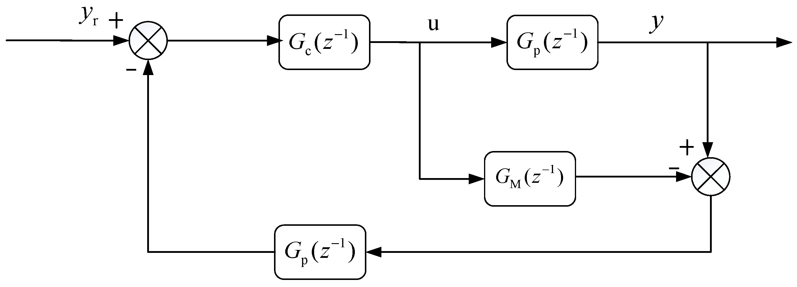
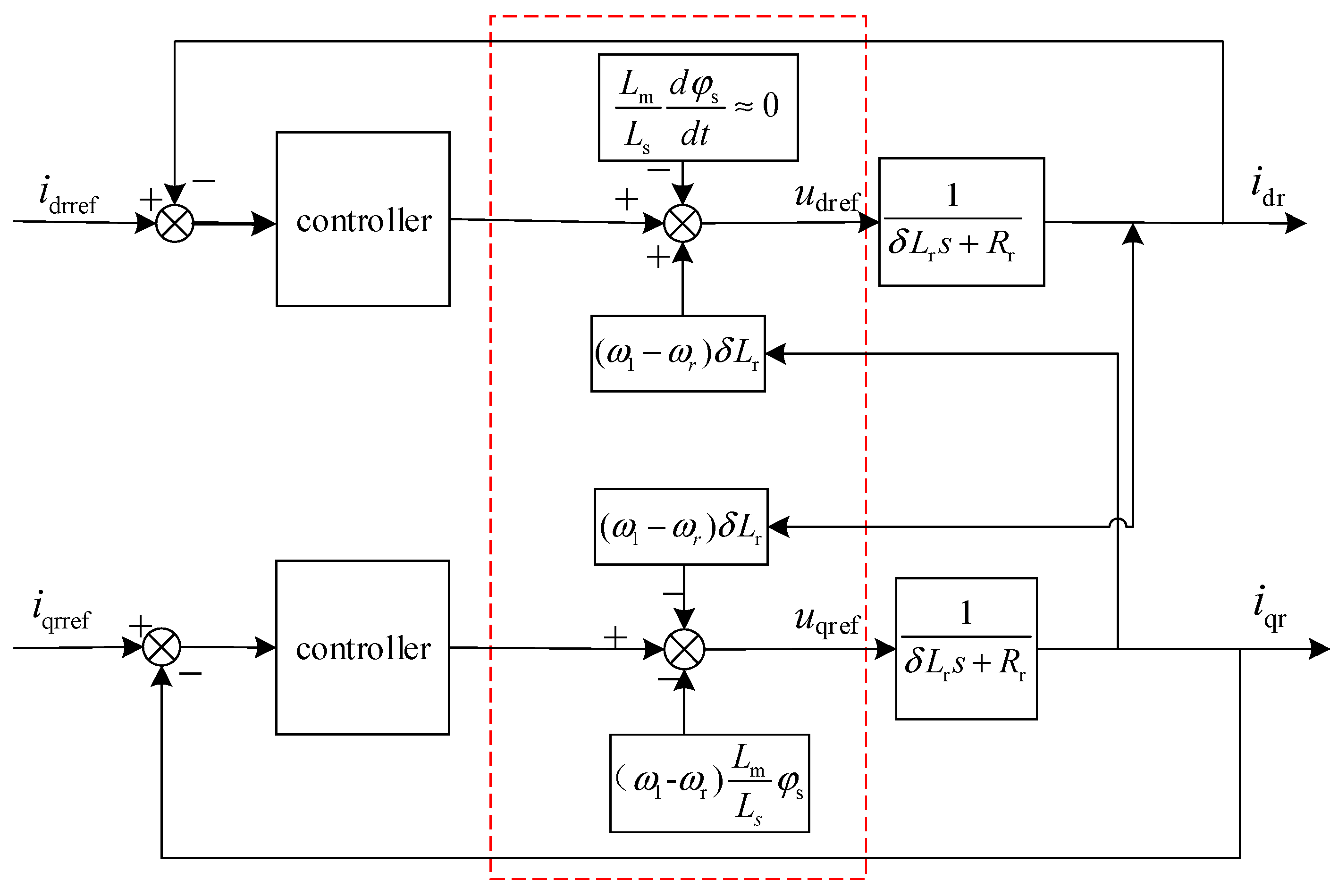
A significant observation is that there exists pronounced cross-coupling and interference between the transfer functions governing the rotor current control. These are primarily caused by the transformation among different frames. However, these cross-coupling and interference terms can be considered as disturbances. The controller compensates for these disturbances, as illustrated in Figure 7.

$$\left\{\begin{array}{l}\Delta v_{\mathrm{qr}}=({\omega }_1-{\omega }_{\mathrm{r}})\left(\delta L_r{i}_{\mathrm{dr}}+{\displaystyle \frac{L_{\mathrm{m}}}{L_{\mathrm{s}}}}{\phi }_{\mathrm{s}}\right)\hfill \\ \Delta v_{\mathrm{dr}}={\displaystyle \frac{L_{\mathrm{m}}}{L_{\mathrm{s}}}}{\displaystyle \frac{d{\phi }_{\mathrm{s}}}{dt}}-({\omega }_1-{\omega }_{\mathrm{r}})\delta L_r{i}_{\mathrm{qr}}\hfill \end{array}\right.$$

(34)

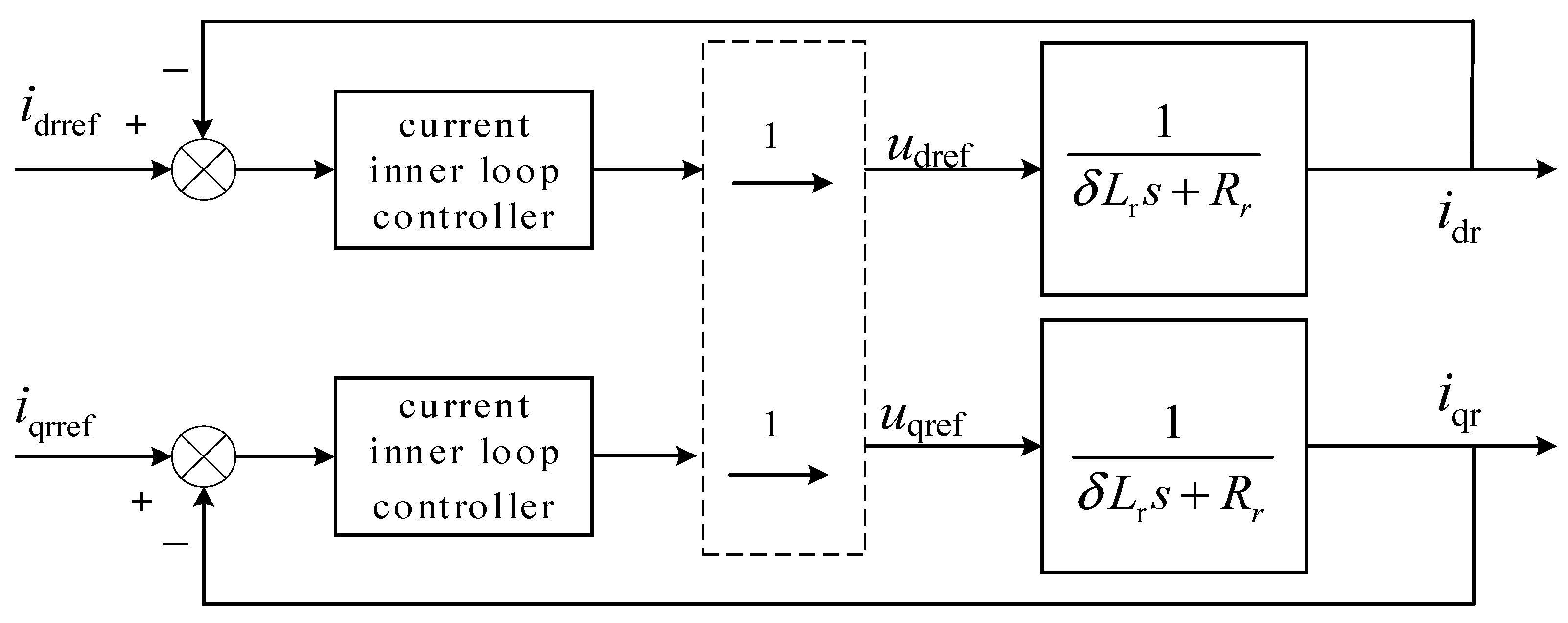
Ignoring the hysteresis generated by the controller, the disturbance term and cross-coupling inherent in the generator model, along with the feed-forward voltage compensation term, can effectively negate each other. Consequently, they can be represented by a straight line with a transfer function of one, further streamlining the structure of the control system. Figure 8 depicts the simplified block diagram depicting rotor current control.

To achieve the desired control characteristics, it is crucial to accurately obtain various parameters. Derivative terms exist in Equation (30). Several systems directly omit this part to avoid disturbances caused by derivatives, potentially failing to achieve full compensation. However, because of the connection between the stator side of the DFIG and the grid, the stator excitation current can be considered constant in a steady state. Thus, the derivative term can be approximated as zero, avoiding scenarios wherein the term does not offer full compensation.

It can be expressed as a transfer function with voltage and current as the input and output, respectively.

$$\begin{array}{l}{G}_d(s)=G_q(s)={\displaystyle \frac{1}{\delta L_{r}s+R_r}}\\ G(s)={\displaystyle \frac{K_c}{S+a_c}}\end{array}$$

(35)

where

$$K_c={\displaystyle \frac{1}{\delta L_r}}a={\displaystyle \frac{R_r}{\delta L_r}}\delta ={\displaystyle \frac{1-L_M^2}{L_r{L}_s}}$$

The GPC CARIMA model of DFIG can be expressed as follows:

$$(1+a{z}^{-1})\Delta i_r(k)=b\Delta u_q(k-1)+c\xi (k)$$

(36)

where ξ(k) represents the noise of the system. According to Equation (8), we obtain

$$\begin{array}{l}A(z^{-1})=(1+a{z}^{-1})\Delta =1+(a-1)z^{-1}-a{z}^{-2}\\ B(z^{-1})=b{z}^{-1} \end{array}$$

(37)

where $b={\displaystyle \frac{K}{\psi }}(1-e^{-\psi T})$, $\psi ={\displaystyle \frac{R_{\mathrm{r}}}{\delta L_{\mathrm{r}}}}$.

(2)

Simulation Verification and Analysis

To validate the effectiveness of the proposed controller, a simulation model of the DFVSPSU was developed in the simulation software, grounded in the control method and model. The designed nonlinear GPC controller was implemented for excitation control on the rotor side of the DFIG. Simulations were performed under different operating conditions. In comparing the control results of the traditional controller to those of the GPC controller, the viability of the designed controller is evident. The parameters for both the PI controller and the GPC controller were optimized using the GA intelligent algorithm by drawing upon actual operational data from a pumped storage power station in China. The parameters are listed in

Table 1. Parameters of the doubly fed motor.

Rated Power/MW	Rated Speed/(r/min)	Rs/pu	Rr/pu	Lm/pu	Ls/pu	Lr/pu	2H/s
300	428.6	0.023	0.016	2.9	3.08	3.06	9.64

,

Table 2. PI controller parameters.

Parameter	Active Power	Reactive Power
KP	3.8	5.4
KI	45	40

and

Table 3. GPC controller parameters.

N1	N2	Nu	λ	α	β
1	5	2	0.987	0.7	0.15

, and α and β are obtained by optimization.

In addition, in order to set the optimal parameters of PID, the objective function is defined as follows:

J = 80 × overshoot + ITAE. (J = A × overshoot + B × ITAE)

where overshoot is the overshoot percentage of the system response, which directly affects the stability. ITAE (integral time absolute error) measures the cumulative error of dynamic system regulation and reflects speed and accuracy.

In this study, the weight of overshoot (A = 80) is much higher than ITAE (B = 1) because the core goal of the paper is to improve the dynamic response and avoid overshoot and oscillation.

Where λ denotes the forgetting factor. In principle, the value of the forgetting factor ranges from 0 to 1, but it is mostly between 0.9 and 1, which can effectively cope with the time-varying system of parameters [29]. When the value is one, the algorithm becomes a simple least squares identification method.

β is an incremental factor, and the control increment is multiplied by a beta factor at every moment solved by the usual generalized predictive control algorithm, adding an adjustable control quantity β, which can be adjusted to increase the stability of the system.

α is the output flexibility coefficient, the value of which is between 0 and 1, which has a great influence on the stability of the closed-loop system. In general, the smaller the value of α, the faster the system reaches the set value, but it is easy to overshoot and cause system instability. Although the system stability is good, the response time is too long; therefore, the response speed should be considered, while the system stability should be compatible.

(1)

10% power disturbance

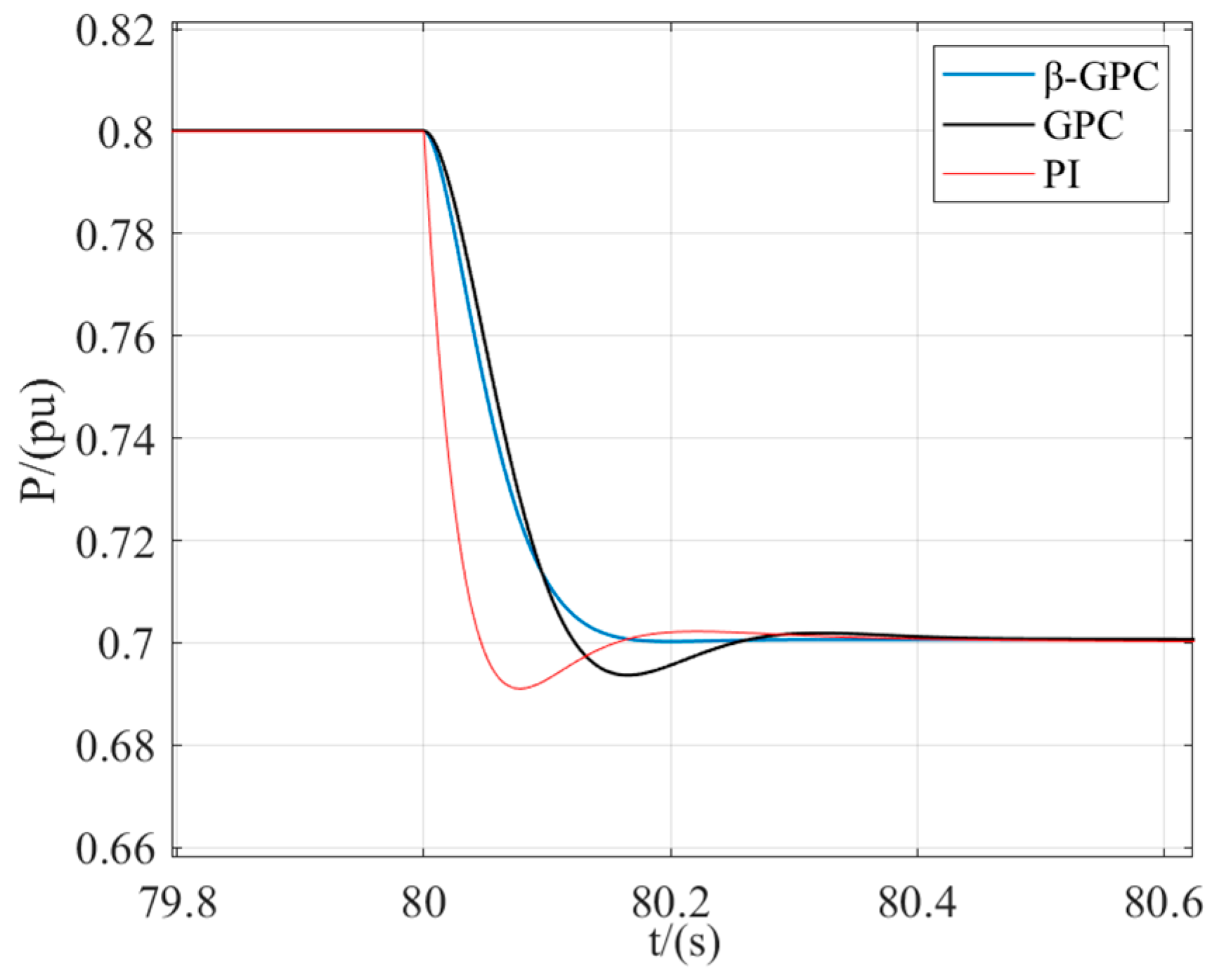
Initially, the simulation conditions were set with the following parameters: the power of the DFVSPSU at 0.8 pu, the head at 1.0 pu, the speed measures at 0.955 pu, and the generator operates with an efficiency of 96.1%. After 80 s, the reference power changes from 0.8 pu to 0.7 pu.

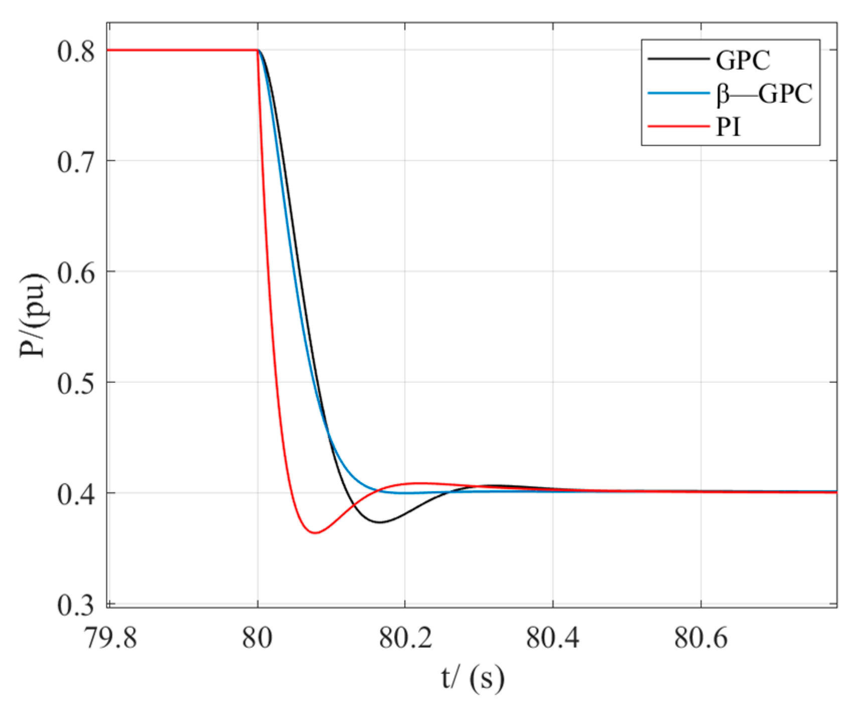
Figure 9 illustrates the operations of the DFSPUS under a 10% power disturbance with different control strategies. The conventional PI controller requires 0.46 s to stabilize, with an overshoot of 9.2% and a single oscillation. However, the traditional GPC controller stabilizes in 0.34 s and reduces the overshoot to 6.1%. In contrast, the improved GPC controller drastically shortens the settling time to 0.2 s, and it does not exhibit any overshoot or oscillations.

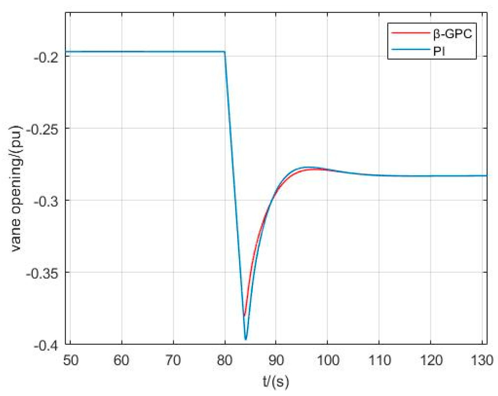
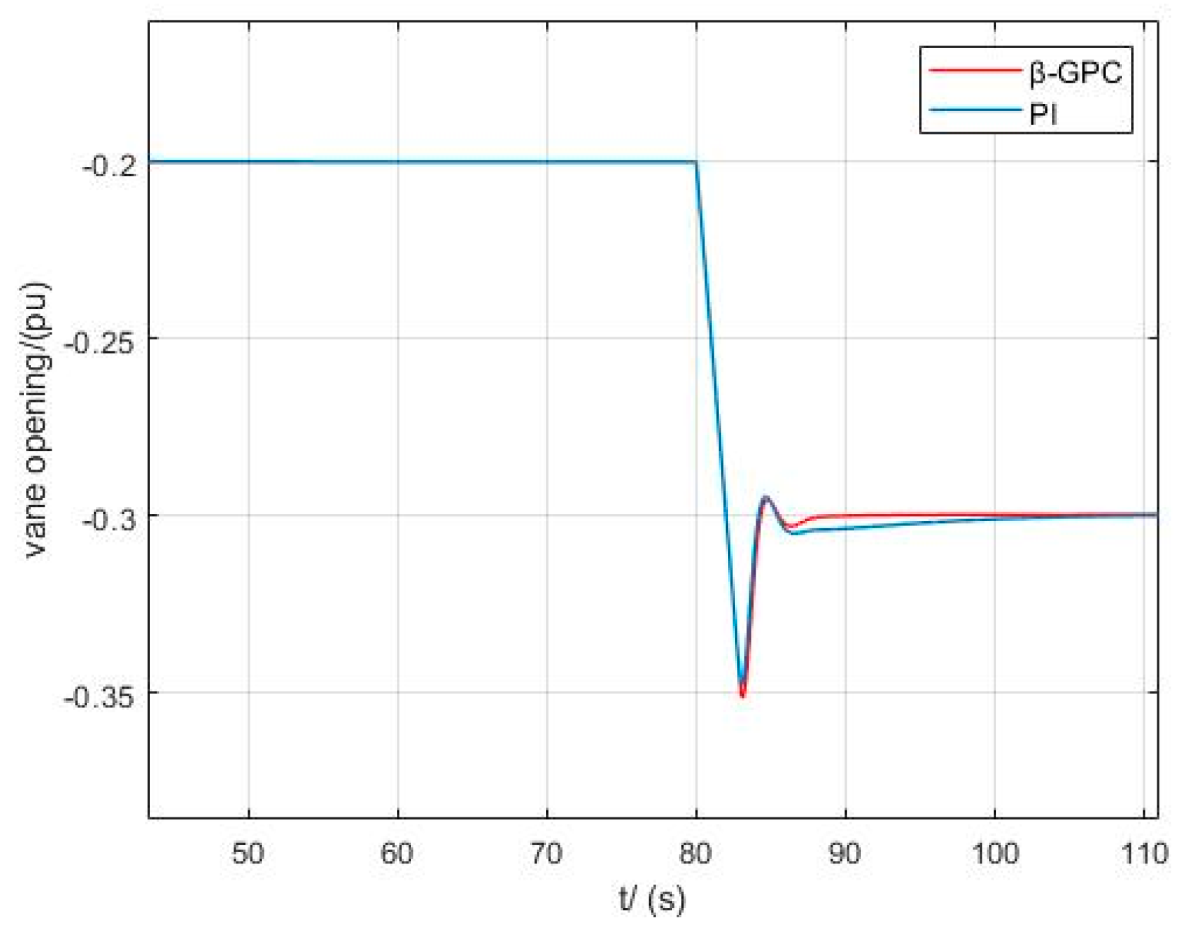
Figure 10 shows the variation of guide vane opening with different control strategies under 10% power interference. Both the traditional PI control and β-GPC control require 28 s to reach stability, but the β-GPC control has advantages over the traditional PI control in terms of overshoot.

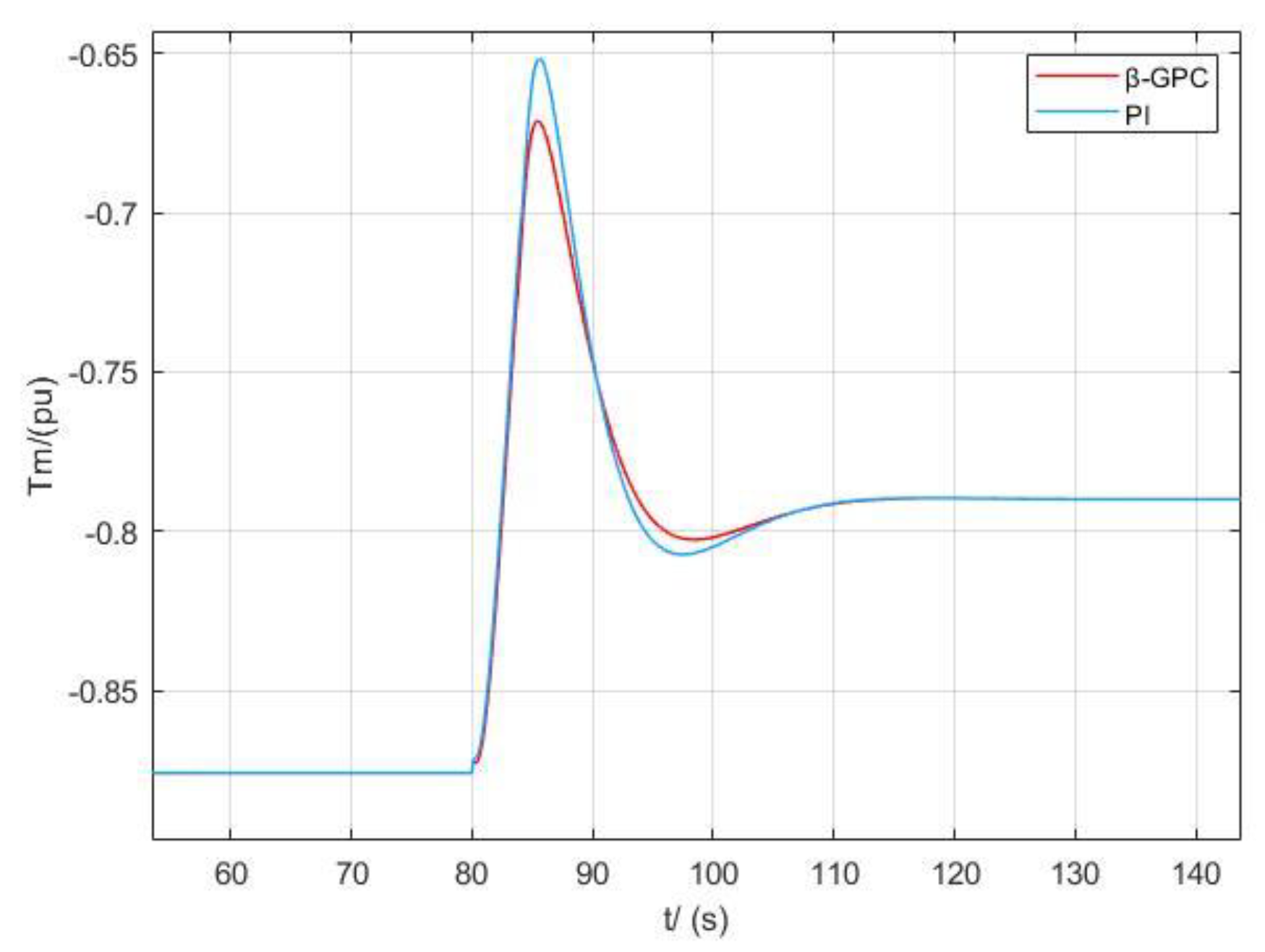
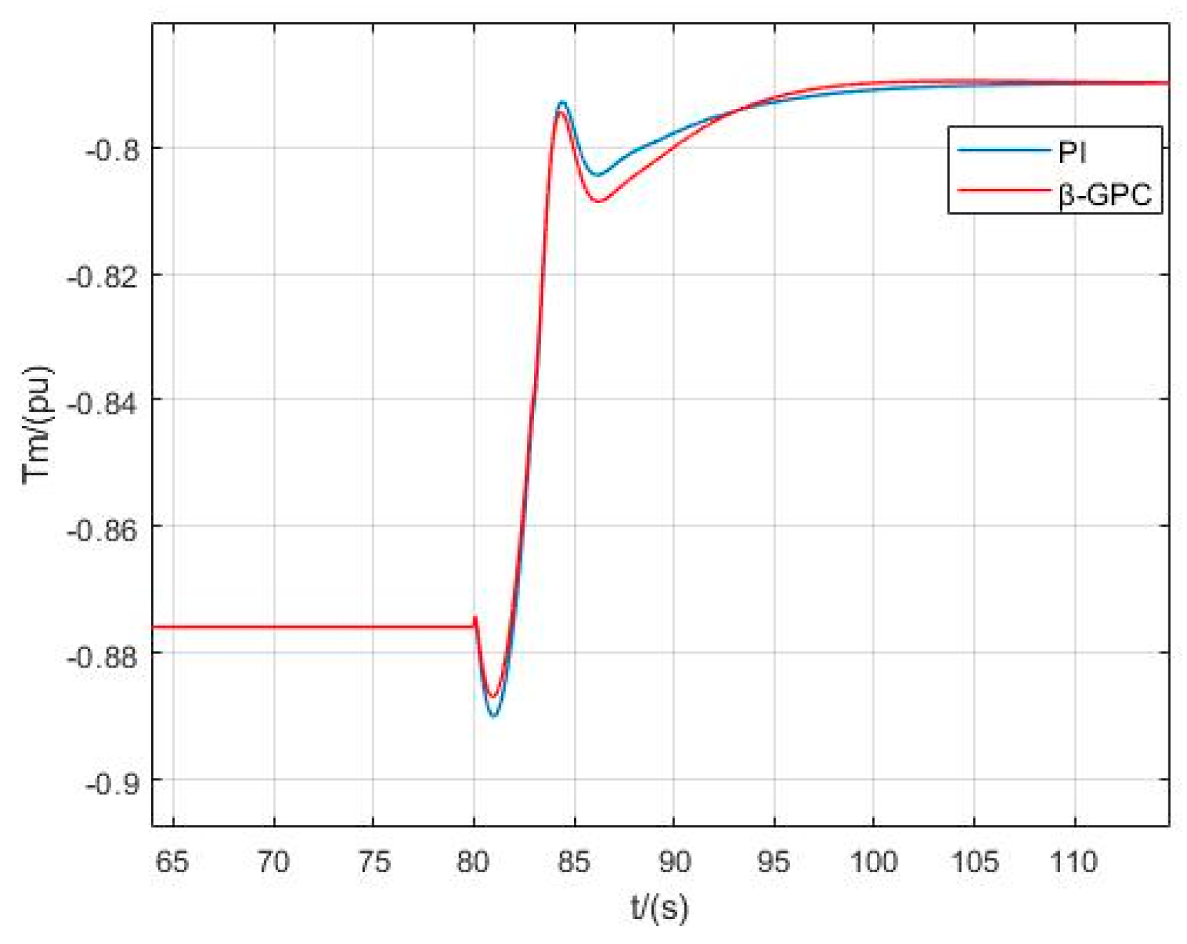
Figure 11 shows the change in the torque of different control strategies under 10% power interference. Both the traditional PI control and the β-GPC control require 35 s to stabilize, but the β-GPC control has advantages over the traditional PI control in terms of overshoot.

Figure 12 presents a comparison of the q-axis current error values, indicating that the improved GPC controller outperforms in terms of control effects. It offers a shorter settling time and fewer oscillations than the traditional PI controller.

(2)

40% power disturbance

The initial simulation conditions are established with the following parameters: the output of the DFVSPSU is 0.8 pu, the head stands at 1.0 pu, the speed measures at 0.955 pu, and the generator has an efficiency of 96.1%. At 80 s, the power reference value steps from 0.8 pu to 0.4 pu.

Figure 13 presents the operations of DFSPUS using different control strategies under a 40% power disturbance. It can be seen that β-GPC control strategy is significantly better than PI controller and traditional GPC controller in terms of stability time and overshoot.

According to the values of the objective function J in

Table 4. Performance comparison of different controllers for adjustment.

	Overshoot (%)	Settling Time (s)	Oscillations	ITAE	J
PI (10%)	9.2	0.46	1	335.2476	1071.2476
GPC (10%)	6.1	0.34	1	333.9506	821.9506
β-GPC (10%)	0	0.2	0	327.8672	327.8672
PI (40%)	9.1	0.48	1	73.9330	801.933
GPC (40%)	6.6	0.38	1	744.6889	1272.6889
β-GPC (10%)	0	0.18	0	744.0486	744.0486

, it can be seen that under 10% and 40% power disturbance conditions, the control performance of the β-GPC controller is significantly better than that of the traditional PI and GPC controllers. Specifically, β-GPC achieves the lowest J value across all test conditions, which fully demonstrates its superior overall performance in overshoot suppression and dynamic error optimization, achieving an optimal balance between control accuracy and response speed.

In the aforementioned simulation verification, we compared the performance of traditional PI controllers, GPC controllers, and the improved β-GPC controller under different power disturbances. The results demonstrate that the improved β-GPC controller outperforms conventional controllers in terms of settling time, overshoot, and oscillation frequency. These performance enhancements are not only reflected in the dynamic response of the system, but also have significant implications for mechanical stress and converter losses in actual operation.

During the operation of doubly-fed induction generators (DFIGs), adjusting the rotor excitation through converters to achieve variable-speed operation is critical. However, during rapid power regulation (such as grid frequency modulation demands), the instantaneous imbalance between electromagnetic torque and mechanical torque exacerbates fluctuations. Particularly under low-load conditions, hydraulic instabilities in the turbine flow passage—such as vortices and flow separation—can induce random torque pulsations. These pulsations are transmitted to the DFIG rotor through the runner-shaft system, generating alternating torsional stress. When the pulsation frequency approaches the natural frequency of the shaft, torsional resonance may occur, amplifying stress amplitudes by three to five times. Furthermore, during variable-speed processes, torque fluctuations are transmitted to the generator set through couplings, subjecting bearings to asymmetric loads. Long-term torque fluctuations can lead to fatigue crack propagation in critical components such as shafts and blades.

Additionally, the stator current amplitude of DFIGs varies significantly with load changes, and the IGBT switching losses exhibit a quadratic relationship with the current. Harmonics in the motor current can also interact with the switching frequency of IGBTs in the converter, triggering high-frequency oscillatory currents. High-frequency components near the IGBT switching frequency increase the current rate of change (di/dt), thereby significantly raising switching losses. Therefore, precise control of motor current is essential for reducing converter switching losses.

The improved β-GPC controller effectively mitigates torque fluctuations and current errors through precise torque control and current tracking. This not only enhances the dynamic response performance of the system, but also significantly reduces mechanical stress and switching losses. Specifically, accurate torque control minimizes asymmetric loads on shafts and bearings, preventing torsional resonance, while precise current control reduces IGBT switching losses, improving overall system efficiency and reliability.

4.2. GPC Controller Design for Outer Speed Loop of DFVSPSU

Based on current research for the control strategy of DFVSPSU, the speed master control approach exists in addition to the power master control method. The speed master control approach involves controlling speed via the excitation control system while managing power through the guide vane governing the system.

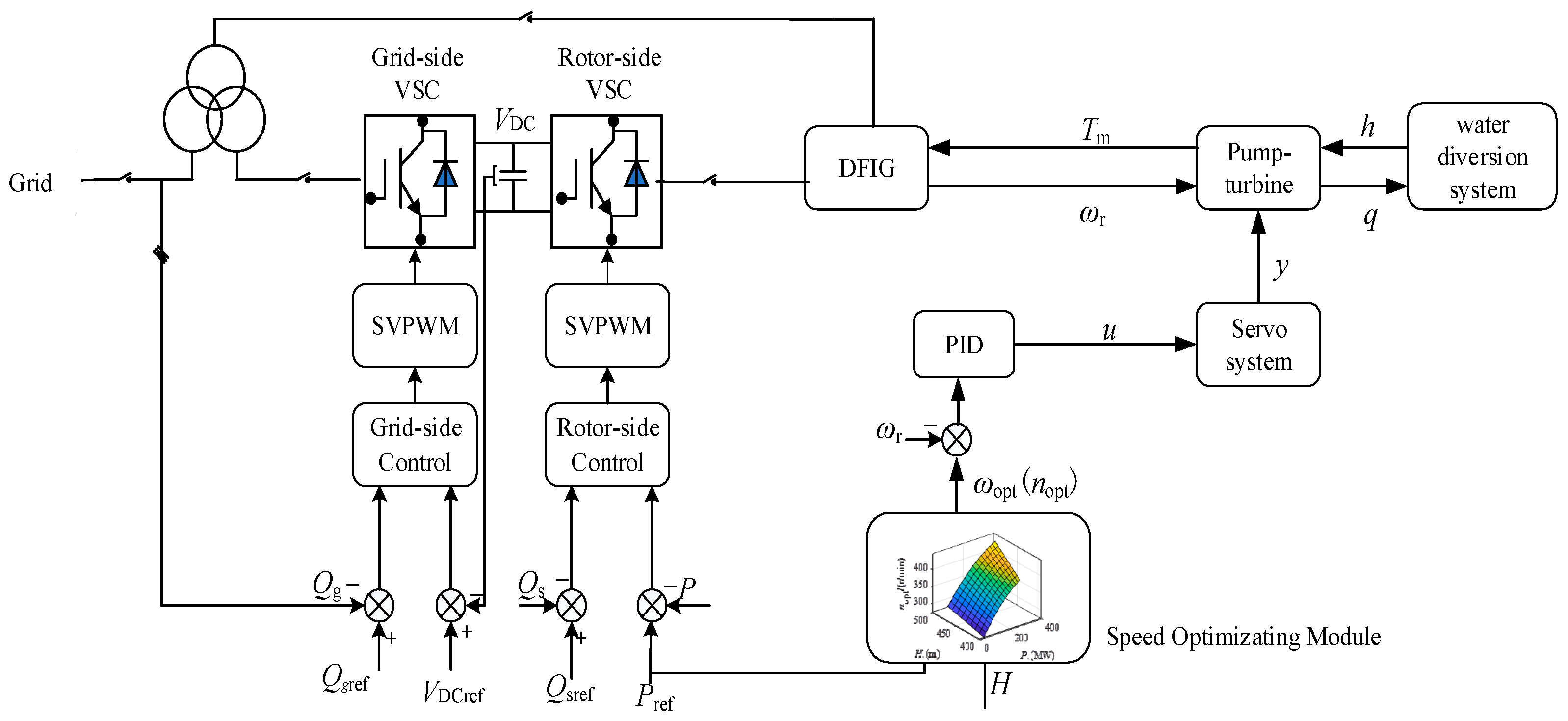
Within this method, any change in the power reference value prompts the optimal speed generator to determine the optimal speed that correlates with optimal efficiency. It is determined using the comprehensive characteristic curve of the pump turbine and the given reference power. The speed of the unit is swiftly adjusted to match the optimal speed reference via excitation control. A notable advantage of the speed master control method is its ability to fine-tune the load regulation of the DFVSPSU. This ensures the pump turbine consistently operates at its highest hydraulic efficiency, improving the overall efficiency of the pumped storage system. Meanwhile, the guide vane governing the system makes adjustments to stabilize the unit’s power around the set reference power. The control strategy for the speed master control method is depicted in Figure 14.

The difference between ω_erf and the actual feedback value is obtained by the PI controller to obtain the rotor side Q-axis current reference value i_qrref, and then it is compared to the actual feedback value; through the second PI controller and the voltage compensation term Δv_dr, the rotor side voltage reference value v_qrref is finally obtained. In the control process of rotor side reactive power, the difference between Q_ref and the actual feedback value is obtained by the PI controller to obtain the rotor side D-axis current reference value i_drref, and then compared to the actual feedback value, through the second PI controller and the voltage compensation term Δv_qr, finally obtaining the rotor side voltage reference value of v_drref. v_qrref and v_drref are transformed by 2r/2s to obtain v_αrref and v_βrref, and then the converter switch signal is obtained by SVPWM.

The power outer loop transformation equation is

$$\left\{\begin{array}{l}{i}_{\mathrm{qrref}}={\displaystyle \frac{L_{\mathrm{s}}}{L_{\mathrm{m}}}}(k_{\mathrm{P}1}+{\displaystyle \frac{k_{\mathrm{I}1}}{s}})({\omega }_{\mathrm{ref}}-\omega )\hfill \\ i_{\mathrm{drref}}={\displaystyle \frac{L_{\mathrm{s}}}{L_{\mathrm{m}}}}(k_{\mathrm{P}3}+{\displaystyle \frac{k_{\mathrm{I}3}}{s}})(Q_{\mathrm{ref}}-Q)-{\displaystyle \frac{{\phi }_1}{L_{\mathrm{m}}}}\hfill \end{array}\right.$$

(38)

The current inner loop transformation equation is

$$\left\{\begin{array}{l}{v}_{\mathrm{qrref}}=(k_{\mathrm{P}2}+{\displaystyle \frac{k_{\mathrm{I}2}}{s}})(i_{\mathrm{qrref}}-i_{\mathrm{qr}})+\Delta v_{\mathrm{dr}}\hfill \\ v_{\mathrm{drref}}=(k_{\mathrm{P}4}+{\displaystyle \frac{k_{\mathrm{I}4}}{s}})(i_{\mathrm{drref}}-i_{\mathrm{dr}})+\Delta v_{\mathrm{qr}}\hfill \end{array}\right.$$

(39)

(1)

Control Strategy Design of Outer Speed Loop

When considering the friction coefficient of DFVSPSU, the motion equation is

$$T_{\mathrm{e}}-T_{\mathrm{L}}-B_{\mathrm{m}}{\omega }_{\mathrm{r}}={\displaystyle \frac{J}{n_{\mathrm{p}}}}{\displaystyle \frac{d{\omega }_{\mathrm{r}}}{dt}}$$

(40)

where T_L denotes the mechanical torque of the prime mover, ω_r symbolizes the speed of the prime mover, J signifies the rotational inertia of the unit, and B_m denotes the viscous friction coefficient. When adopting the control strategy with i_d = 0,

$$T_{\mathrm{e}}=1.5n_{\mathrm{p}}\left({\phi }_{\mathrm{ds}}{i}_{\mathrm{qs}}-{\phi }_{\mathrm{qs}}{i}_{\mathrm{ds}}\right)$$

(41)

$$T_{\mathrm{e}}=K{i}_{\mathrm{q}}$$

(42)

Thus, when the mechanical torque is zero, the model obtained by taking the Laplace change on both sides of the equation is

$$(K{i}_{\mathrm{q}}-B_{\mathrm{m}}{\omega }_{\mathrm{r}})/J={\displaystyle \frac{d{\omega }_{\mathrm{r}}}{dt}}$$

(43)

$$G(s)={\displaystyle \frac{K}{Js+B}}$$

(44)

Here, the input and output are the speed and current, respectively, after adding zero-order hold. Z-transform is used to obtain the following

$$G(z)={\displaystyle \frac{b{z}^{-1}}{1+a{z}^{-1}}}$$

(45)

Here, $a=-e^{-TB/J}$ $b=k(1-e^{-TB/J})/J$.

The load torque is regarded as the system disturbance, and then it is added into the equation, and the CARIMA model is constructed as follows:

$$(1+a{z}^{-1})\Delta {\omega }_r(k)=b\Delta {\mathrm{i}}_q(k-1)+c{T}_L(k)\Delta$$

(46)

Hence, the performance index function is

$$J=E\left\{{\left[{\omega }_r-{\omega }_0\right]}^T\left[{\omega }_r-{\omega }_0\right]+\Delta i_q^T\Gamma \Delta i_q\right\}$$

(47)

where ω_r denotes the actual speed and ω₀ is the reference speed. Accordingly, the control quantity is

$$\begin{array}{l}{i}_q(k)=i_q(k-1)+\Delta i_q(k)\\ {=\mathrm{i}}_q(k-1)+\left[1,0,\dots ,0\right]\Delta i_q(k)\end{array}$$

(48)

Thus, the desired CARIMA model and the GPC controller are designed.

(2)

Simulation Verification and Analysis

In the speed master control method, the parameters of the unit involved are the same as those presented in Table 1, and the parameters of different controllers are optimized using the GA intelligent algorithm. The controller parameters are detailed in

Table 5. PI controller parameters.

Parameter	Active Power	Reactive Power
KP	20	20
KI	18	12

and

Table 6. GPC controller parameters.

N1	N2	Nu	λ	α	β
1	8	4	0.976	0.8	0.76

, and α and β are obtained by optimization.

(1)

10% Power Disturbance

The initial simulation conditions are established with the following parameters: the output of the DFVSPSU is 0.8 pu, the head is 1.0 pu, speed is 0.9551 pu, and the generator efficiency is 96.1%. At 80 s, the power reference value steps from 0.8 pu to 0.7 pu.

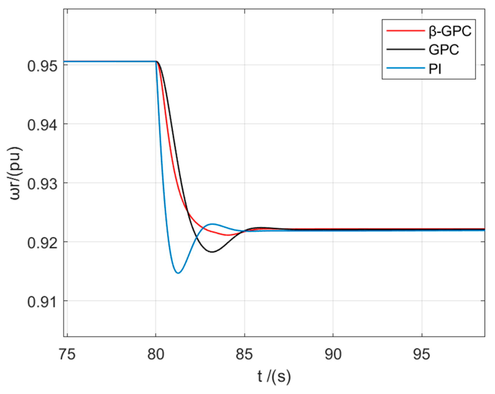
Figure 15 shows the operation of DFVSPSU with different control strategies under 10% power disturbance. The traditional PI controller brings the DFVSPSU to a steady state in 8.48 s, exhibiting an overshoot of 22.4%, and then it undergoes two oscillations. When utilizing the traditional GPC controller, there is a reduction in the settling time of the speed to 7.08 s, and the overshoot decreases to 13.7%. In comparison, the improved GPC controller further decreases the response time by 3.19 s and achieves stabilization without any overshoot or oscillation.

Figure 16 shows the variation of guide vane opening (0.8–0.7) with different control strategies under 10% power interference. The traditional PI control needs 23 s to achieve stability, and the β-GPC control only needs 9 s to achieve stability. There is little difference between the two methods in the performance of overshoot.

Figure 17 shows the change in the torque of different control strategies under 10% power interference. Both the traditional PI control and β-GPC control require 27 s to achieve stability, but the β-GPC control has advantages over traditional PI control in terms of overshoot.

(2)

40% Power Disturbance

At the initial moment, the output of the DFVSPSU is 0.8 pu, the head is 1.0 pu, speed is 0.9551 pu, and the generator efficiency is 96.1%. At 80 s, the power reference value steps from 0.8 pu to 0.4 pu.

Figure 18 shows the operation of DFVSPSU under different control strategies with 40% power disturbance. It can be seen that β-GPC control strategy is significantly better than PI controller and traditional GPC controller in terms of stability time and overshoot.

Table 7. Performance comparison of different controllers when adjusting.

	Overshoot (%)	Settling Time (s)	Oscillations	ITAE	J
PI (10%)	22.4	8.48	2	290.4264	2082.4264
GPC (10%)	13.7	7.08	1	571.6804	1667.6804
β-GPC (10%)	3.2	3.9	0	659.0790	915.079
PI (40%)	24.6	15.2	2.5	2303.1512	4271.1512
GPC (40%)	19.8	14.5	1	2327.1073	3911.1073
β-GPC (40%)	0	4.9	0	2466.4382	2466.4382

compares the regulation performance of PI controllers, GPC controllers, and β-GPC controllers under different power disturbance conditions. The numerical values based on the objective function J show that the β-GPC controller demonstrates significant advantages, as follows: under 10% and 40% power disturbances, its J value is significantly lower than those of traditional PI and GPC controllers. These data fully validate the superior performance of β-GPC in overshoot suppression and dynamic regulation.

5. Conclusions

The control system of a DFVSPSU was investigated. Considering the challenges posed by traditional controllers in addressing the strong nonlinearity of the system, the GPC strategy was integrated into the DFVSPSU. The ordinary GPC controller was improved into a β-incremental GPC controller to counter potential model mismatches, especially under large disturbances. Additionally, the recursive least squares method was employed for real-time parameter identification. The research results include the following: When the unit output is compared under different power instruction steps, the traditional PI controller needs about 0.48 s at most to achieve stability and have a certain number of oscillations. The control time of the traditional GPC controller is shorter than that of the PI controller, requiring up to 0.38 s, and the overshoot is also reduced from up to 9.2% to 6.6%. In contrast, the improved β-GPC controller can stabilize the unit in as little as 0.2 s without overshoot and subsequent oscillations. It can be seen that the proposed controller is superior to the traditional controller, especially in reducing the stability time, oscillation, and overshoot, thus verifying the effectiveness of the proposed controller. In addition, the newly designed controller also has certain limitations, such as the fact that the controller is highly dependent on the accuracy and speed of the parameter identification algorithm; if the error of the parameter identification is large, it can affect the final control result. The shortcomings are the direction of our follow-up research.

References

1. Kougias, I.; Aggidis, G.; Avellan, F.; Deniz, S.; Lundin, U.; Moro, A.; Muntean, S.; Novara, D.; Pérez-Díaz, J.I.; Quaranta, E.; et al. Analysis of emerging technologies in the hydropower sector. Renew. Sustain. Energy Rev. 2019, 113, 109257. [Google Scholar] [CrossRef]
2. Iliev, I.; Trivedi, C.; Dahlhaug, O.G. Variable-speed operation of Francis turbines: A review of the perspectives and challenges. Renew. Sustain. Energy Rev. 2019, 103, 109–121. [Google Scholar] [CrossRef]
3. Valavi, M.; Nysveen, A. Variable-speed operation of hydropower plants: A look at the past, present, and future. IEEE Ind. Appl. Mag. 2018, 24, 18–27. [Google Scholar] [CrossRef]
4. Jabr, H.M.; Lu, D.; Kar, N.C. Design and implementation of neuro-fuzzy vector control for wind-driven doubly-fed induction generator. IEEE Trans. Sustain. Energy 2011, 2, 404–413. [Google Scholar] [CrossRef]
5. Merabet, A.; Eshaft, H.; Tanvir, A.A. Power-current controller based sliding mode control for DFIG-wind energy conversion system. IET Renew. Power Gener. 2018, 12, 1155–1163. [Google Scholar] [CrossRef]
6. Bounar, N.; Labdai, S.; Boulkroune, A. PSO–GSA based fuzzy sliding mode controller for DFIG-based wind turbine. ISA Trans. 2019, 85, 177–188. [Google Scholar] [CrossRef] [PubMed]
7. Litao, D.; Jian, G.; Shoudao, H.; Xianglong, T. Variable speed constant frequency hydropower technology and its development. Electr. Power Syst. Autom. 2020, 44, 169–177. [Google Scholar]
8. Shao, Y.; Ji, L.; Yuan, Y.; Gao, S. Self-starting scheme of variable speed pumped storage unit under pumping conditions. Autom. Electr. Power Syst. 2016, 40, 125–130+156. [Google Scholar]
9. Xijun, Z.; Jinghuan, D.; Yifan, H.; Weijia, Y.; Jiebin, Y.; Jiandong, Y. Speed increase law of variable speed pumped storage unit under large fluctuation conditions. J. Hydroelectr. Power Gener. 2021, 40, 57–64. [Google Scholar]
10. Beltran, B.; Benbouzid, M.E.H.; Ahmed-Ali, T. Second-order sliding mode control of a doubly fed induction generator driven wind turbine. IEEE Trans. Energy Convers. 2012, 27, 261–269. [Google Scholar] [CrossRef]
11. Kumar, R.; Kumar, A. Optimal scheduling of variable speed pumped storage, solar and wind energy system. Energy Sources Part A: Recover. Util. Environ. Eff. 2021, 47, 5225–5239. [Google Scholar] [CrossRef]
12. Feng, C.; Zheng, Y.; Li, C.; Mai, Z.; Wu, W.; Chen, H. Cost advantage of adjustable-speed pumped storage unit for daily operation in distributed hybrid system. Renew. Energy 2021, 176, 1–10. [Google Scholar] [CrossRef]
13. Fang, H.; Chen, L.; Li, X. Comparison of PID parameter optimization of hydraulic turbine governor based on linear and nonlinear models. Chin. J. Electr. Eng. 2010, 30, 100–106. [Google Scholar]
14. Zhou, T.; Zhou, J.; Chang, L. Application of Fuzzy Control in Water Turbine Regulating System. J. Power Syst. Autom. 2003, 1, 10–14+81. [Google Scholar]
15. Xiong, J.; Shi, H.; Wang, T. Optimal control and Modeling analysis of Hydraulic Turbine Speed Control System based on Fractional Order PID Hybrid Algorithm. Water Electr. Energy Sci. 2020, 38, 163–167. [Google Scholar]
16. Wang, R.; Yang, L.; Wang, G. Water turbine regulating system adaptive sliding mode control strategy. People Yangtze River 2023, 7, 234–238+244. [Google Scholar] [CrossRef]
17. Ben Khedher, N.; Boudjemline, A.; Aich, W.; Zeddini, M.A.; Calderon-Madero, J.E. Statistical quality control based on control charts and process efficiency index by the application of fuzzy approach (case study: Ha’il, Saudi Arabia). Water Sci. Technol. 2023, 87, 3146–3163. [Google Scholar] [CrossRef]
18. Troudi, F.; Jouini, H.; Mami, A.; Ben Khedher, N.; Aich, W.; Boudjemline, A.; Boujelbene, M. Comparative Assessment between Five Control Techniques to Optimize the Maximum Power Point Tracking Procedure for PV Systems. Mathematics 2022, 10, 1080. [Google Scholar] [CrossRef]
19. Chen, J.; Zhou, B. Power grid load forecasting based on improved Generalized Predictive control based on BP artificial neural network. J. Chifeng Inst. (Nat. Sci. Ed.) 2019, 35, 62–64. [Google Scholar] [CrossRef]
20. Xiao, Z.; Liu, N.; Zhang, Y.; Chai, T. Nonlinear generalized predictive control method based on parameter optimization and compensation signal. Sci. China Inf. Sci. 2019, 54, 2240–2262. (In Chinese) [Google Scholar] [CrossRef]
21. Song, Y.; Ran, H. Turbine based on generalized predictive control system frequency regulation research. J. Henan Univ. Technol. (Nat. Sci. Ed.) 2022, 9, 103–111. [Google Scholar] [CrossRef]
22. Chen, J.; Liu, S.; Wang, Y.; Hu, W.; Zou, Y.; Zheng, Y.; Xiao, Z. Generalized predictive control application scheme for nonlinear hydro-turbine regulation system: Based on a precise novel control structure. Energy 2024, 296, 130916. [Google Scholar] [CrossRef]
23. Gao, C. Optimal Control and Stability Analysis of Doubly Fed Variable Speed Pumped Storage Unit. Ph.D. Thesis, Xi’an University of Science and Technology, Xi’an, China, 2022. [Google Scholar] [CrossRef]
24. Lin, C.; Wang, F.; Yao, X. Research on Excitation Control Technology of Variable Speed Constant Frequency doubly fed Wind Turbine. Proc. CSEE 2003, 11, 126–129. [Google Scholar]
25. Hu, Y.; Jia, X. A review of generalized predictive control. Inf. Control. 2000, 3, 248–256. [Google Scholar]
26. Wang, W.; Yang, J. Generalized predictive control: Theory, algorithm and application. Control Theor. Appl. 1997, 6, 777–786. [Google Scholar]
27. Wang, W. A direct method of generalized predictive adaptive control. Acta Autom. Sin. 1996, 3, 270–277. [Google Scholar]
28. Wang, H.; Li, Z.S. Multi-Area Load Frequency Control in Power System Integrated With Wind Farms Using Fuzzy Generalized Predictive Control Method. IEEE Trans. Reliab. 2022, 72, 737–747. [Google Scholar] [CrossRef]
29. Xun, Q.; Wang, P.; Li, Z. Parameter identification of permanent magnet Servo System based on recursive least square Method. Trans. China Electrotech. Soc. 2016, 31, 161–169. [Google Scholar]
30. Shi, W.; Shao, C.; Sun, Z. Improved GPC network control algorithm based on AR model delay prediction. Control Decis. 2012, 27, 477–480. [Google Scholar]
31. Chen, Z.Q.; Wu, X.; Sun, M.W.; Sun, Q.L. Stability analysis of active disturbance rejection generalized predictive control in frequency domain. J. Harbin Eng. Univ. 2018, 39, 1046–1051. [Google Scholar]
32. Mao, Z.; Chen, Z.; Sun, Q.; Yuan, Z. Frequency-domain-based stability analysis of generalized predictive controller (GPC). Control. Decis. 2002, 17, 859–862. [Google Scholar]
33. Yang, C. Research on Control Method of Doubly Fed Wind Power System. Ph.D. Thesis, University of Science and Technology Beijing, Beijing, China, 2019. [Google Scholar]
34. Cui, J. Research on Robust Control of Permanent Magnet Synchronous Motor for Vehicles Based on Generalized Predictive Control. Master’s Thesis, Kunming University of Science and Technology, Kunming, China, 2021. [Google Scholar]
35. Rahimi, M. Analysis of grid-side converter dynamics and Dc-link controller design in DFIG-based wind turbines. J. Energy Manage 2016, 6, 16–27. [Google Scholar]
36. Zhou, N.; Sun, F.; Wang, Q.; Meng, X. A flexible power control strategy for rotor-side converter of DFIG under unbalanced grid voltage sags. Int. J. Electr. Power Energy Syst. 2017, 90, 64–75. [Google Scholar] [CrossRef]
37. Liu, Y.; Wang, Z.; Xiong, L.; Wang, J.; Jiang, X.; Bai, G.; Li, R.; Liu, S. DFIG wind turbine sliding mode control with exponential reaching law under variable wind speed. Int. J. Electr. Power Energy Syst. 2018, 96, 253–260. [Google Scholar] [CrossRef]
38. Takahashi, I.; Noguchi, T. A new quick-response and high-efficiency control strategy of an induction motor. IEEE Trans. Ind. Appl. 1986, IA-22, 820–827. [Google Scholar] [CrossRef]
39. Depenbrock, M. Direct self-control (DSC) of inverter-fed induction machine. IEEE Trans. Power Electron. 1988, 3, 420–429. [Google Scholar] [CrossRef]
40. Buja, G.; Kazmierkowski, M. Direct torque control of PWM inverter-fed AC motors—A survey. IEEE Trans. Ind. Electron. 2004, 51, 744–757. [Google Scholar] [CrossRef]
Figure 1. Pump turbine curve obtained by the logarithmic projection method. (a) x − Q11 curve; (b) x − M11 curve.
Energies 18 02904 g001
Figure 2. Servo system model.
Energies 18 02904 g002
Figure 3. Circuit structure diagram of grid-side converter.
Energies 18 02904 g003
Figure 4. Control block diagram of the hydraulic turbine working condition of doubly fed variable-speed unit.
Energies 18 02904 g004
Figure 5. GPC internal mold structure diagram.
Energies 18 02904 g005
Figure 6. Rotor-side vector control block diagram of the power master control method.
Energies 18 02904 g006
Figure 7. Voltage feed-forward compensation rotor current control block diagram.
Energies 18 02904 g007
Figure 8. Simplified block diagram of rotor current control with voltage feed-forward compensation.
Energies 18 02904 g008
Figure 9. Active power of different controllers at 10% power disturbance.
Energies 18 02904 g009
Figure 10. Comparison of guide vane opening under 10% power disturbance.
Energies 18 02904 g010
Figure 11. Comparison of torque under 10% power disturbance.
Energies 18 02904 g011
Figure 12. Comparison of current error values at 10% power disturbance.
Energies 18 02904 g012
Figure 13. Active power of different controllers at 40% disturbance.
Energies 18 02904 g013
Figure 14. Rotor-side vector control block diagram of speed main control method.
Energies 18 02904 g014
Figure 15. Speed comparison at 10% power disturbance.
Energies 18 02904 g015
Figure 16. Comparison of guide vane opening under 10% power disturbance.
Energies 18 02904 g016
Figure 17. Comparison of torque under 10% power disturbance.
Energies 18 02904 g017
Figure 18. Speed comparison at 40% power disturbance.
Energies 18 02904 g018