
Optimisation of Dynamic Operation Strategy for a Regional Multi-Energy System to Reduce Energy Congestion

Abstract
1. Introduction
- (1)
- This study investigates a practical regional multi-energy system with the characteristics of energy congestion.
- (2)
- A TRNSYS-based optimisation model is developed to simulate dynamic optimisation strategies to reduce the actual monitoring data collection and analysis.
- (3)
- A two-stage loading strategy is proposed for optimising the system operation.
2. Materials and Methods
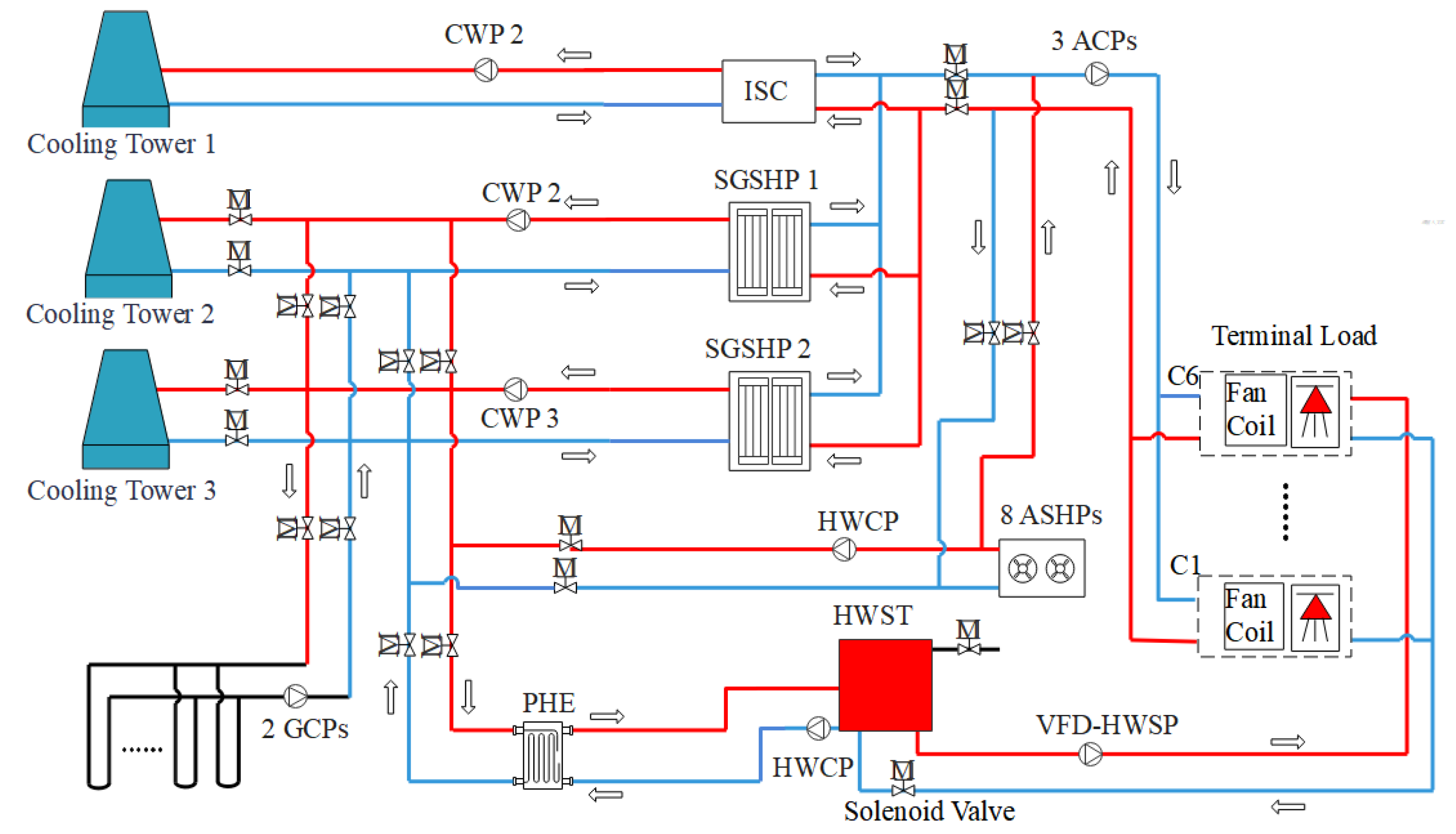
2.1. Overview of Multi-Source Regional Energy Systems
2.2. System Parameters and Evaluation Indicators
- 1.
- The unit instantaneous cooling/heating capacity Q (kW) is
- 2.
- The electric power W (kW) is
- 3.
- The unit cooling/heating coefficient of performance COPj is
- 4.
- The system cooling/heating coefficient of performance COPs is
- 5.
- Part Load Ratio PLR:
3. Energy Consumption Analysis of Regional Multi-Energy System
3.1. Cooling Energy Consumption Analysis of Regional Multi-Energy System
3.1.1. Cooling Energy Consumption Analysis of the Whole System
3.1.2. COP of Each Unit Under Different Loads
3.2. Heating Energy Consumption Analysis of the Regional Multi-Energy System
3.3. Analysis of Cooling and Heating Power Consumption in the Regional Multi-Energy System
4. Numerical Simulation
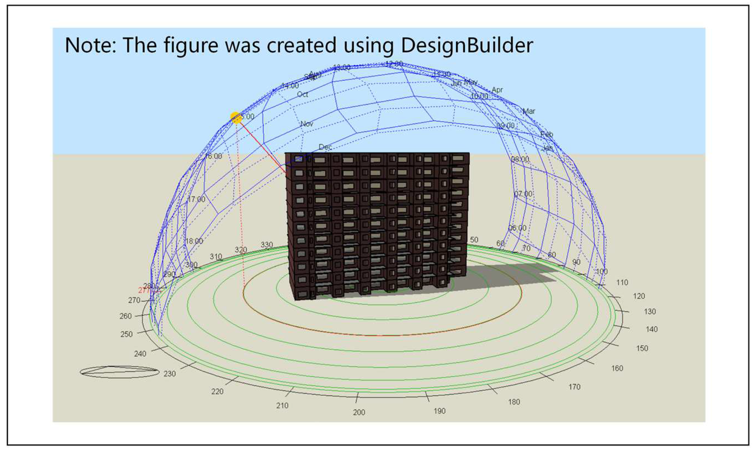
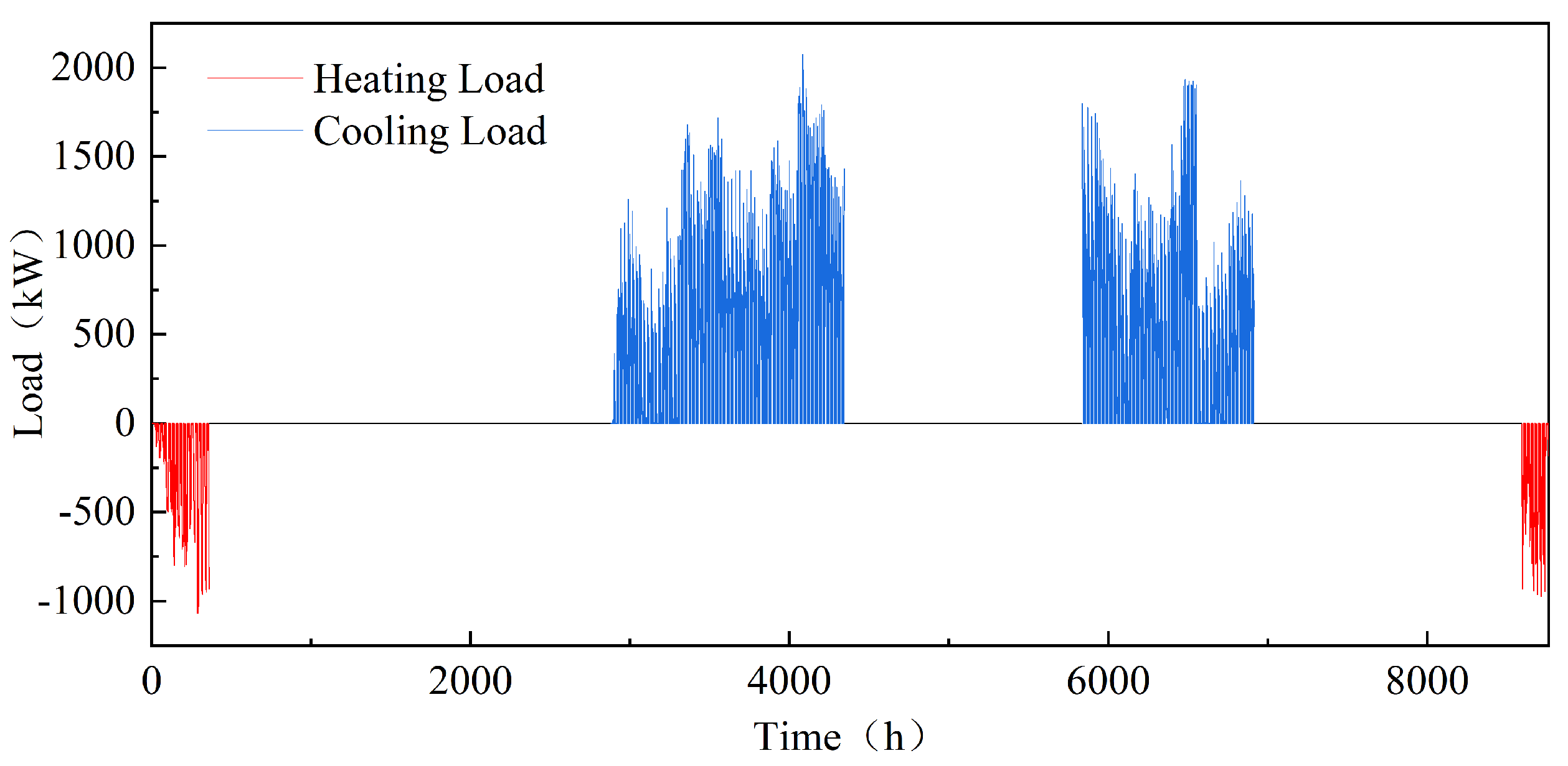
4.1. Building Cooling and Heating Load Simulation
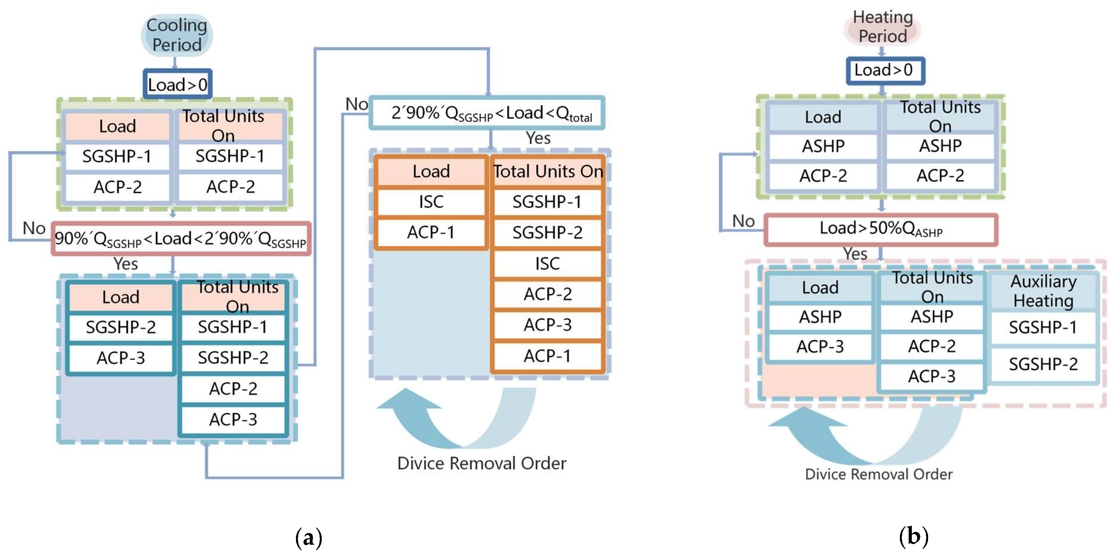
4.2. Unit Optimisation Operation Control Strategy Based on Dynamic Load
4.3. Simulation Parameters
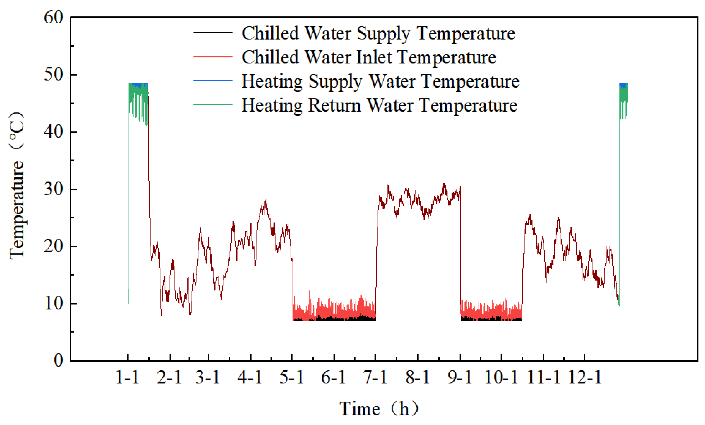
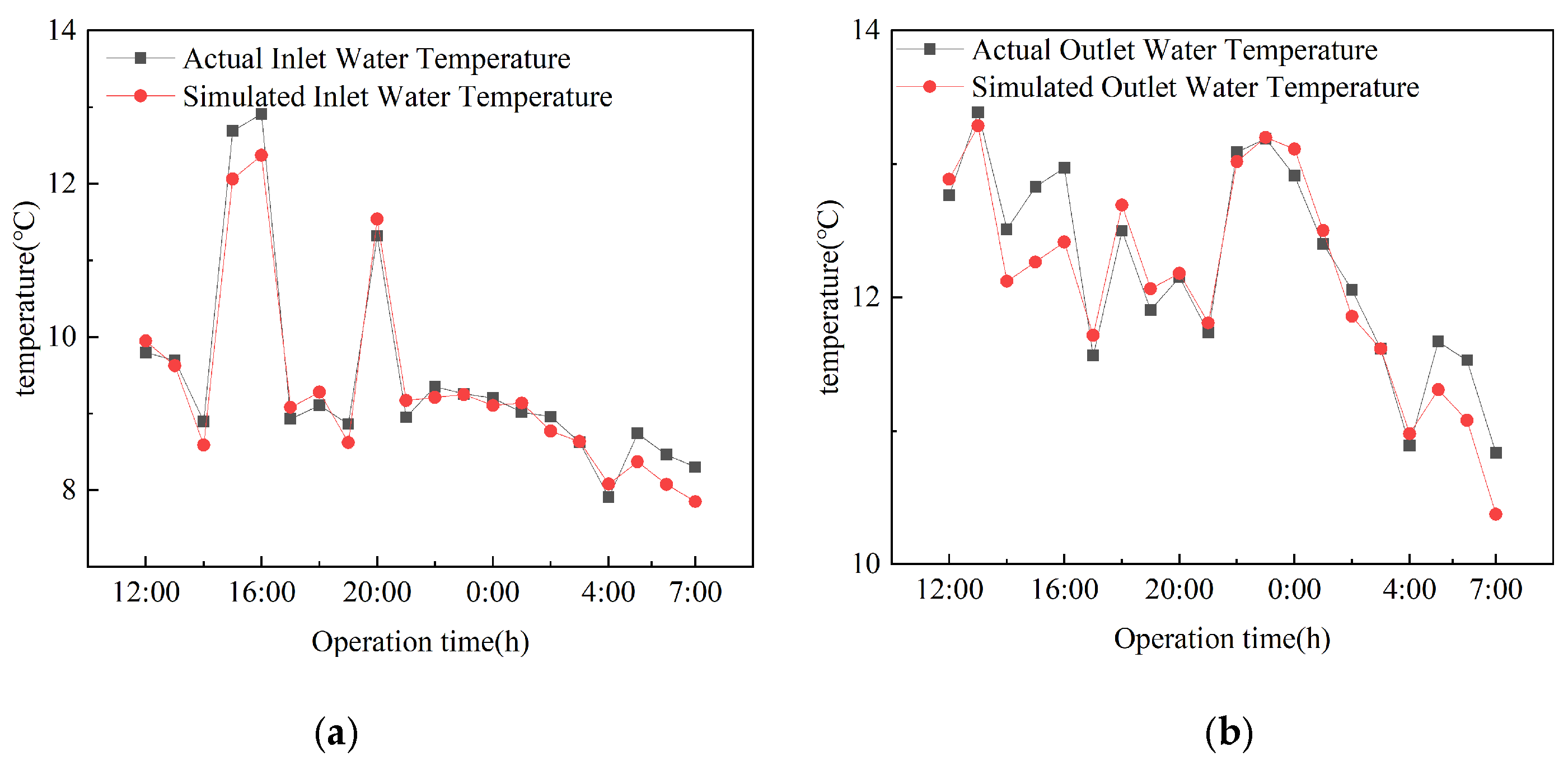
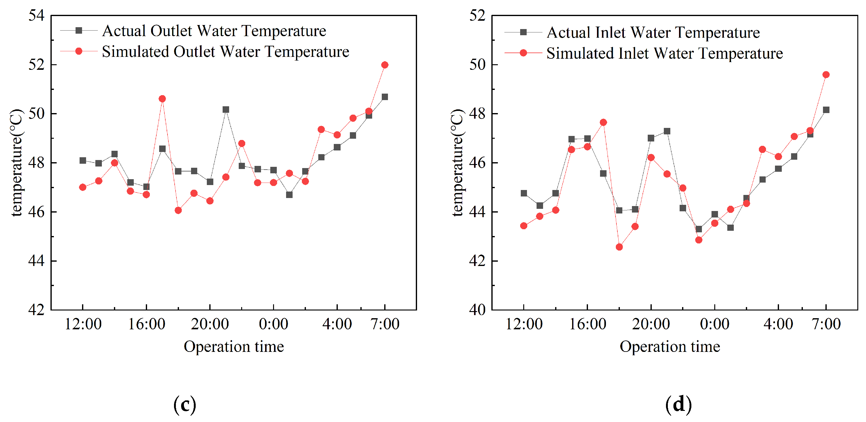
4.4. Model Validation
4.5. Error Calculation
- 1.
- Absolute Error
- 2.
- Mean Error
- 3.
- Root Mean Squared Error [23]
- 4.
- Coefficient of Determination
5. System Simulation Results
5.1. Simulation of the Regional Multi-Energy System Under the Original Operation Strategy
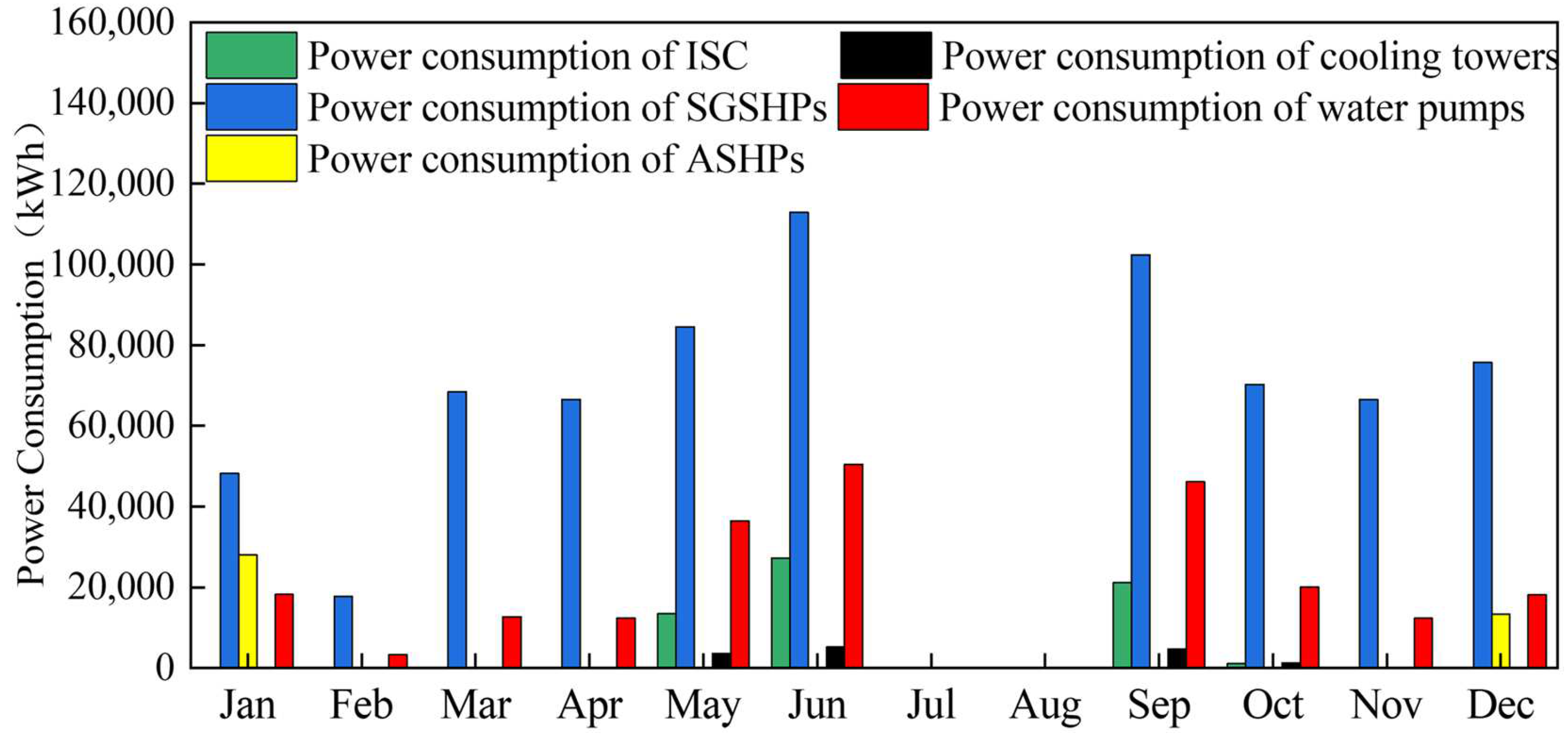
5.2. Power Consumption of Each Device Before and After Optimisation
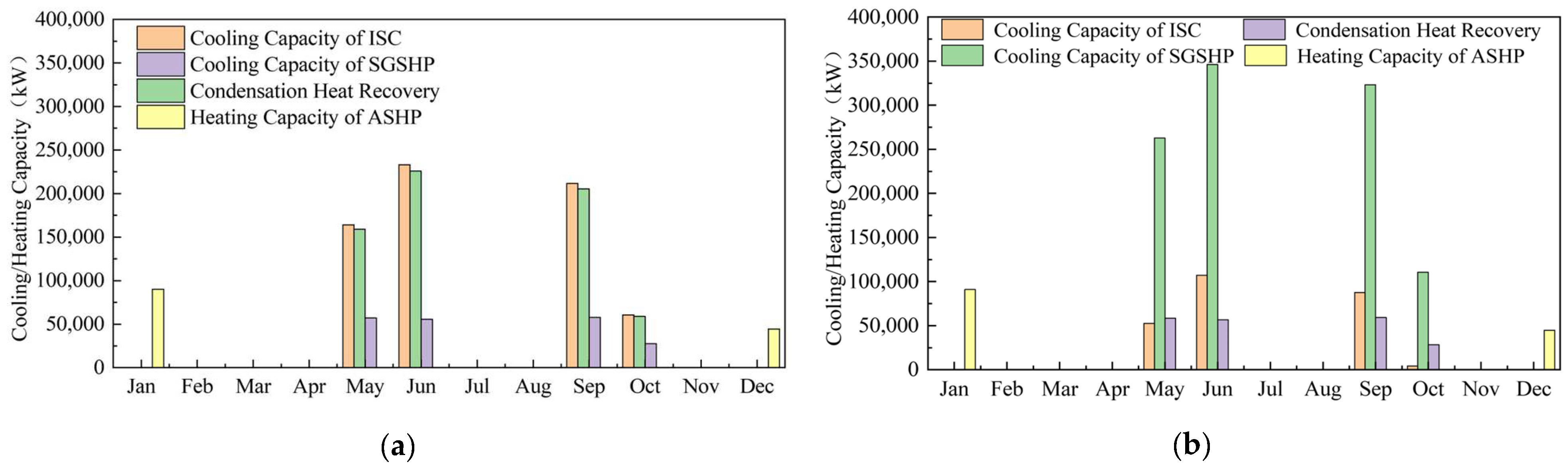
5.3. Cooling/Heating Capacity of Each Device Before and After Optimisation
6. Conclusions
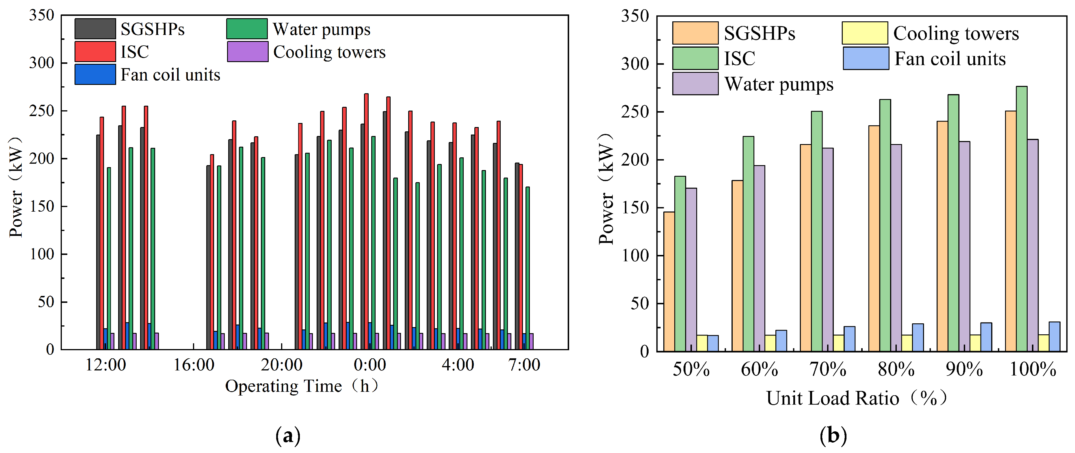
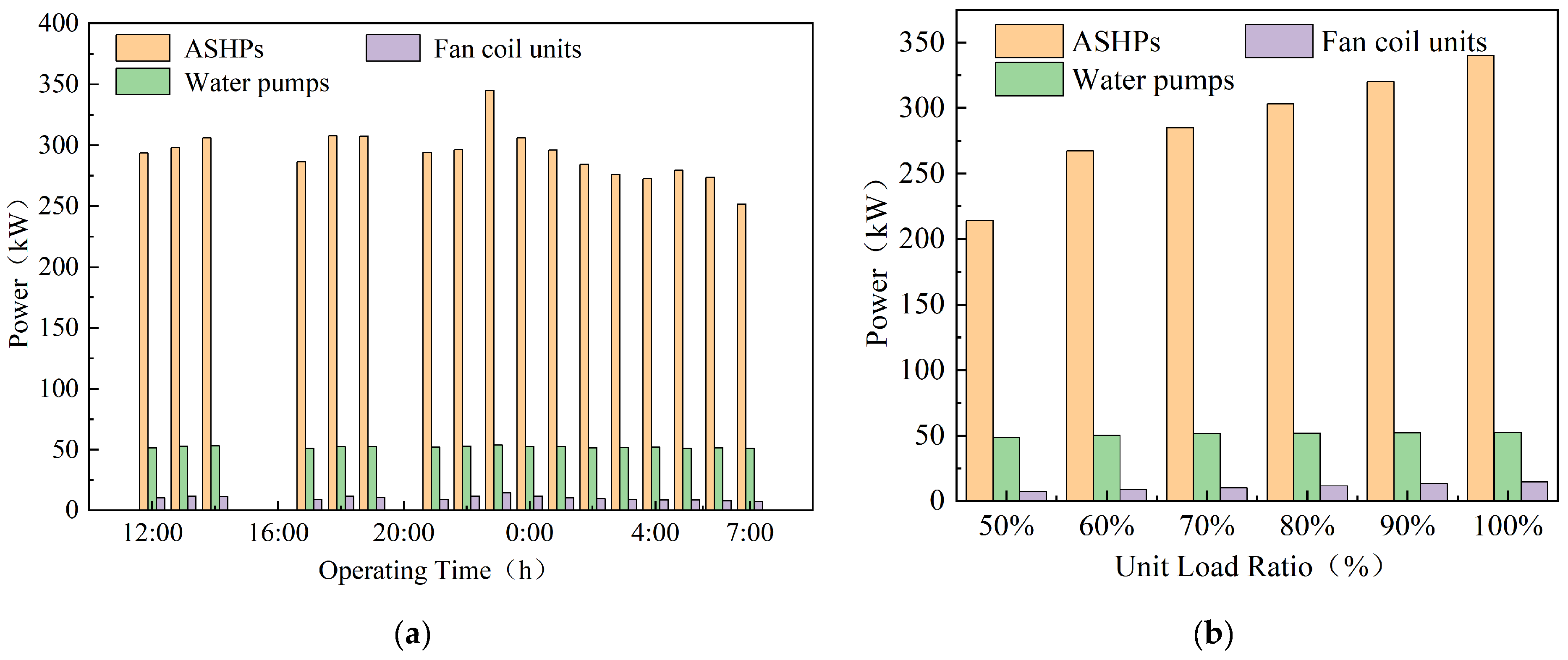
- For the practical regional multi-energy system, the power consumption of the units and pumps increased as the unit load increased for air-conditioning cooling. However, the proportion of power consumed by the units increased by 4.15%, while the proportion of the water pump’s power decreased by 4.24%. At a unit load ratio of 90%, COPSGSHP and COPSGSHPS reached maximum values of 4.4 and 3.2, respectively. During system heating, the power consumption of the ASHPs continuously increased for the unit load ratio range of 50–100%, and their share of the total power consumption increased. The proportion of all the water pumps and FCUs of the total power consumption also significantly decreased. A reasonable unit load ratio enhances the unit’s operating efficiency, and 90% was recommended under the conditions in this paper.
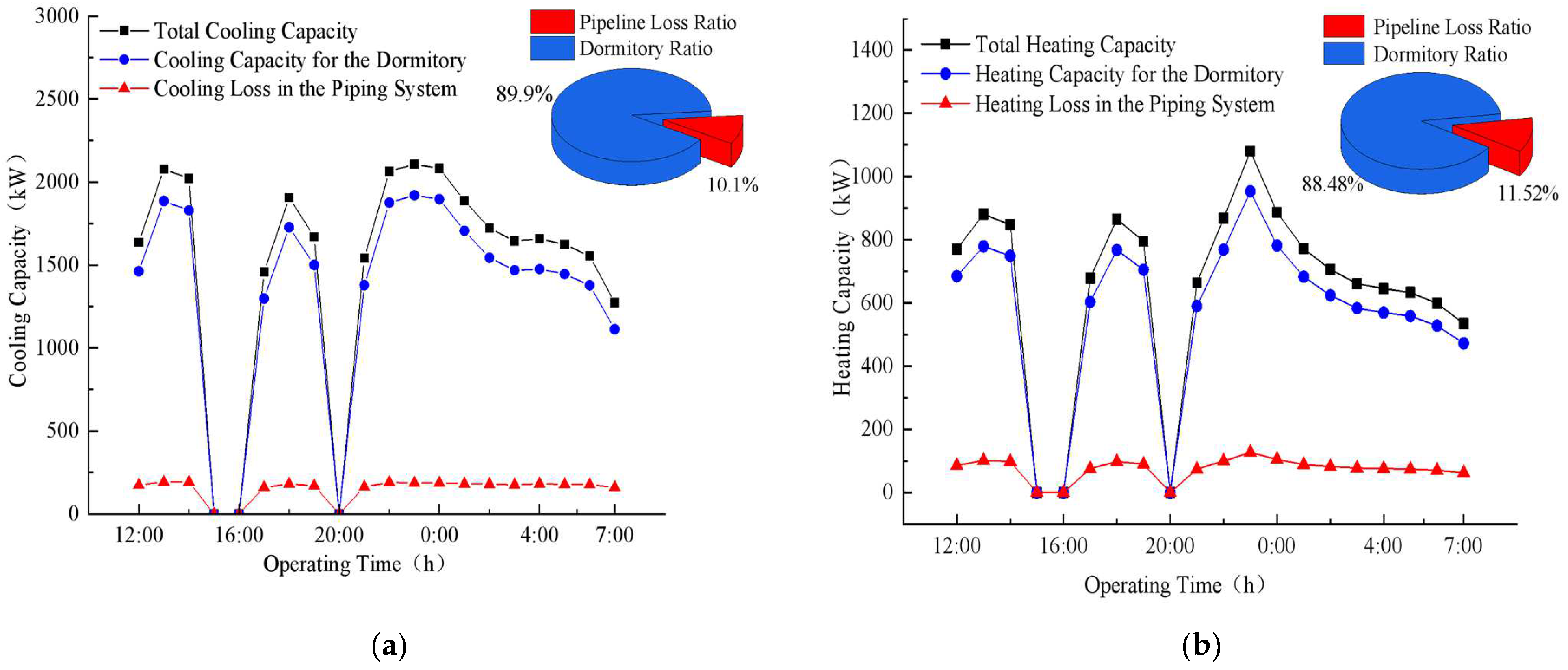
- For the practical regional multi-energy system, the daily use of the cooling capacity was approximately 89.76% of the total cooling capacity, with pipeline losses of around 10.24%. The power consumption of the water pumps was significantly higher than that of the regional multi-energy system for heat dissipation and terminal air-conditioning equipment. The daily use of the heating capacity was approximately 88.5% of the total heating capacity, with pipeline losses of around 11.5%.
- The DesignBuilder software was used to simulate the cooling and heating load of the building’s terminal air-conditioning system. Based on the simulation results from DesignBuilder, a two-stage loading strategy for ISC operation based on dynamic loads has been proposed.
- A TRNSYS building simulation model was established based on the optimisation operation control strategy. After optimisation, the total running time of all units decreased by 28.83%, with the chiller unit’s operating time decreasing the most, approximately 80.04%. The total power consumption of the optimised system decreased by about 19%, and the power consumption of all units throughout the year increased by 6.68% compared to the original operation strategy, which indicated that the unit’s operating efficiency was improved. The cooling/heating capacity of the optimised system changed little, and the system still met the terminal load requirements. Furthermore, the condensate heat recovery during the cooling season increased by about 2.3%.
7. Limitations and Future Research
- Due to the limitations of experimental conditions, the data of the system’s annual performance were mainly based on simulation results. Long-term data monitoring should be carried out under permissible conditions to compare the fitting degree between simulation results and measured results, thereby enhancing the reliability of the simulation.
- During certain months of the year, college students stopped using air conditioning but still used the domestic hot water. This paper mainly focuses on the system’s power consumption during the season that the air conditioning was in use. The analysis of the system’s operation should be expanded to domestic hot water coupled with air conditioning in the future.
Author Contributions
Funding
Data Availability Statement
Conflicts of Interest
Abbreviations
| Items | Full name |
| ACP | Air-conditioning pump |
| ACPs | Air-conditioning pumps |
| ASHP | Air-source heat pump |
| ASHPs | Air-source heat pumps |
| ASHPS | Air-source heat pump system |
| COP | Coefficient of performance |
| CT | Cooling tower |
| CTs | Cooling towers |
| CWP | Cooling water pump |
| CWPs | Cooling water pumps |
| FCU | Fan coil unit |
| GCP | Geothermal circulation pump |
| GCPs | Geothermal circulation pumps |
| GHE | Geothermal heat exchanger |
| GSHP | Ground-source heat pump |
| GSHPS | Ground-source heat pump system |
| HVAC | Heating, ventilation, and air-conditioning |
| HWCP | Hot water circulation pump |
| HWST | Hot water storage tank |
| ISC | Integrated screw chiller |
| ISCS | Integrated screw chiller system |
| PHE | Plate heat exchanger |
| PLR | Part load ratio |
| PV | Photovoltaic |
| RES | Regional energy system |
| SGSHP | Screw ground-source heat pump |
| SGSHPs | Screw ground-source heat pumps |
| SGSHPS | Screw ground-source heat pump system |
| VFD-HWSP | Variable frequency drive hot water supply pump |
References
- Han, J.; Zhao, H.; Hu, X. Reliability evaluation of regional integrated energy system considering multiple energy storage resources. In Proceedings of the 2020 IEEE 16th International Conference on Control & Automation (ICCA), Singapore, 9–11 October 2020; pp. 436–441. [Google Scholar]
- Abimbola, S.A.; Wanning, M. The status and potential of regional integrated energy systems in sub-Saharan Africa: An Investigation of the feasibility and implications for sustainable energy development. Energy Strategy Rev. 2024, 53, 101402. [Google Scholar]
- Wang, X.; Li, T.; Yu, Y. Performance simulation and energy efficiency analysis of multi-energy complementary HVAC system based on TRNSYS. Appl. Therm. Eng. 2024, 257, 124378. [Google Scholar] [CrossRef]
- Chika, K.; Mika, Y. Long-term operation analysis of a ground source heat pump with an air source heat pump as an auxiliary heat source in a warm region. Energy Build. 2023, 289, 113050. [Google Scholar]
- West, S.R.; Ward, J.K.; Wall, J. Trial results from a model predictive control and optimisation system for commercial building HVAC. Energy Build. 2014, 72, 271–279. [Google Scholar] [CrossRef]
- Alirahmi, S.M.; Rahmani, D.S.; Ahmadi, P. Multi-objective design optimization of a multi-generation energy system based on geothermal and solar energy. Energy Convers. Manag. 2020, 205, 112426. [Google Scholar] [CrossRef]
- Tang, W.T. Operation optimization of regional integrated energy systems. Energy Sci. Eng. 2023, 11, 4542–4556. [Google Scholar] [CrossRef]
- Kavei, F.A.; Nicoli, M.; Quatraro, F.; Savoldi, L. Enhancing energy transition with open-source regional energy system optimization models: TEMOA-Piedmont. Energy Convers. Manag. 2025, 327, 119536. [Google Scholar] [CrossRef]
- Yang, T.; Wang, Q.C. Low-carbon economic distributed dispatch for district-level integrated energy system considering privacy protection and demand response. Appl. Energy 2025, 383, 125389. [Google Scholar] [CrossRef]
- Lu, M.X.; Teng, Y. A bi-level optimization strategy of electricity-hydrogen-carbon integrated energy system considering photovoltaic and wind power uncertainty and demand response. Sci. Rep. 2025, 15, 18. [Google Scholar] [CrossRef]
- Jiao, X.N.; Wu, J.K. An optimal method of energy management for regional energy system with a shared energy storage. Energies 2023, 16, 886. [Google Scholar] [CrossRef]
- Porsani, G.B.; Casquero-Modrego, N.; Trueba, J.B.E.; Bandera, C.F. Empirical evaluation of EnergyPlus infiltration model for a case study in a high-rise residential building. Energy Build. 2023, 296, 113322. [Google Scholar] [CrossRef]
- Maryam, K.; Hajar, A. Energy and exergy analysis of the transient performance of a qanat-source heat pump using TRNSYS-MATLAB co-simulato. Energy Environ. 2023, 34, 560–585. [Google Scholar]
- Qu, Y.; Wang, F.; Wang, Y.; Wang, P.; Li, T.; Meng, Z.F. Simulation Optimization and Experiment of R1234-ze on the Heat Pump Water Heater Storage Tank. Adv. Mater. Res. 2014, 1051, 828–831. [Google Scholar] [CrossRef]
- Leila, A.; Umberto, B. Dynamic simulation of a hydrogen-fueled system for zero-energy buildings using TRNSYS software. E3S Web Conf. 2023, 396, 04005. [Google Scholar]
- Dai, Z.; Zhang, X.; Liu, J.; Liu, B.; Tang, F. Energy-saving control strategy for the joint operation of multiple ground source heat pumps system based on TRNSYS: A research study. Case Stud. Therm. Eng. 2025, 67, 105834. [Google Scholar] [CrossRef]
- Korichi, S.; Bouchekima, B.; Naili, N. Performance analysis of horizontal ground source heat pump for building cooling in arid Saharan climate: Thermal-economic modeling and optimization on TRNSYS. Renew. Energy Environ. Sustain. 2021, 61, 1. [Google Scholar] [CrossRef]
- Wang, Z.; Luther, M.; Horan, P. Residential space heating electrification through a PV-driven hot water heat pump. Energy Build. 2025, 330, 115319. [Google Scholar] [CrossRef]
- Saleem, A.; Loo, U.E.C. Thermal performance analysis of a heat pump-based energy system to meet heating and cooling demand of residential buildings. Appl. Energy 2025, 383, 125306. [Google Scholar] [CrossRef]
- Fu, H.; Li, J.; Wang, X. Performance analysis of water source heat pump air-conditioning system for Haihe River as heat source. Int. J. Refrig. 2025, 171, 38–50. [Google Scholar] [CrossRef]
- Arif, F.; Khan, A.W. Smart Progress Monitoring Framework for Building Construction Elements Using Videography–MATLAB–BIM Integration. Int. J. Civ. Eng. 2021, 19, 717–732. [Google Scholar] [CrossRef]
- Crawley, D.B.; Lawrie, L.K.; Winkelmann, F.C. EnergyPlus: Creating a new-generation building energy simulation program. Energy Build. 2001, 33, 319–331. [Google Scholar] [CrossRef]
- Hodson, T.O. Root-mean-square error (RMSE) or mean absolute error (MAE): When to use them or not. Geosci. Model Dev. 2022, 15, 5481–5487. [Google Scholar] [CrossRef]


| TRNSYS [15] | EnergyPlus [12] | MATLAB [13] | Fluent [14] | |
|---|---|---|---|---|
| Flexibility | High (Modular, strong customization capabilities) | Medium (Limited model expandability) | High (General-purpose programming language) | Medium (Primarily for flow field simulation) |
| Accuracy | High (Dynamic simulation, supported by experimental data) | High (Static simulation) | High (Dependent on user-defined models) | High (For flow field and heat transfer analysis) |
| Dynamic multi-energy system modeling | Very suitable (Rich energy system modules, optimization tools) | Suitable for building energy analysis | Requires self-developed models | Suitable for flow field and heat transfer analysis |
| Integration with other software | Very strong (Integrates with MATLAB, Fluent, etc.) | Strong (Integrates with BIM [21], etc.) | Strong (General interfaces) | Medium (Primarily for CFD analysis) |
| Equipment Name | Equipment Image | Manufacturer | City and Country | Equipment Type | Equipment Rated Power (kW) | Number |
|---|---|---|---|---|---|---|
|
Integrated screw chiller (ISC) |  | Zhejiang Sinoking Air-Conditioning & Refrigeration Co., Ltd | Zhejiang, China | SKCWZ30360ARORRZ(T) | 300 | 1 |
|
Screw ground- source heat pump (SGSHP) | 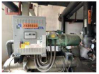 | Climaveneta Chat Union Refrigeration Equipment (Shanghai) Co., Ltd |
Shanghai, China | PSRHH 1651C-Y-R | 101.8 | 2 |
|
Air-source heat pump (ASHP) | 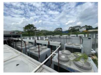 | Zhuhai Gree Electric Appliances Inc. |
Zhuhai, China | KFRS-150FM/A1S | 36.7 | 8 |
|
Geothermal circulation pump (GCP) | 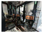 | Nanfang Pump Industry Co., Ltd | Hangzhou, China | TD125-28/4 | 18.5 | 3 |
|
Hot water circulation pump (HWCP) | 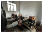 | Nanfang Pump Industry Co., Ltd | Hangzhou, China | TD125-14/4 | 7.5 | 4 |
|
Variable frequency drive hot water supply pump (VFD-HWSP) | 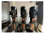 | Nanfang Pump Industry Co., Ltd | Hangzhou, China | CDL42-40-2 | 15 | 3 |
|
Air-conditioning pump (ACP) | 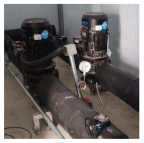 | Nanfang Pump Industry Co., Ltd | Hangzhou, China | LD100-52/2SWHCJ | 30 | 2 |
| Cooling water pump (CWP) | 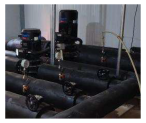 | Nanfang Pump Industry Co., Ltd | Hangzhou, China | LD125-19G/4SWHCJ | 11 | 2 |
| Plate heat exchanger (PHE) | 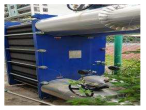 | Guangzhou Saiwell Thermal Equipment Co., Ltd | Guangzhou, China | SWBH200MB-H1200-197-T | / | 1 |
|
Cooling tower (CT) | 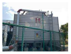 | HON MING Technology Group Co., Ltd | Foshan, China | / | 11 | 3 |
|
Hot water storage tank (HWST) | 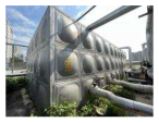 | Guangxi Nanning Tongfa Environmental Protection and Energy-saving Technology Co., Ltd | Nanning, China | 150 m3 | / | 1 |
| Total Cooling/Heating (kWh) | Cooling/Heating for Users (kWh) | Cooling/Heating of Pipeline Loss (kWh) | Proportion of Cooling/Heating Loss | |
|---|---|---|---|---|
| Cooling | 29,927.7 | 26,900.2 | 3027.5 | 10.1% |
| Heating | 12,881 | 11,396.2 | 1484.2 | 11.5% |
| Parameters | Value | Parameters | Value |
|---|---|---|---|
| Longitude | 108.33 °E | Latitude | 22.84 °N |
| Elevation | 72.2 m | Highest dry bulb temperature in winter | 20.1 °C |
| Highest dry bulb temperature in summer | 37 °C | Winter diurnal temperature range | ____ |
| Summer diurnal temperature range | 6.7 °C | Average daily atmospheric pressure in winter | 99,873 Pa |
| Average daily atmospheric pressure in summer | 99,600 Pa | Winter wind speed | 1.3 m/s |
| Summer wind speed | 2.4 m/s | Average monthly radiation in winter | 241.5 MJ/m2 |
| Average monthly radiation in summer | 476.7 MJ/m2 | Average monthly relative humidity in winter | 72% |
| Average monthly relative humidity in summer | 81% | Average monthly moisture content in winter | 7.73 g/kg |
| Average monthly moisture content in summer | 20.12 g/kg | Indoor temperature in winter | 22 °C |
| Indoor temperature in summer | 26 °C | Relative humidity in indoor spaces during winter | ____ |
| Relative humidity in indoor spaces during summer | 60% | Equipment power density | 5 W/m2 |
| Fresh air volume | 24 m3/h | U-value of roof | 0.8 W/(m2·K) |
| Personnel density | 0.25 people/m2 | Solar heat gain coefficient of windows | 0.44 |
| U-value of exterior walls | 1.5 W/(m2·K) | Window-to-wall ratio(south) | 23.56% |
| U-value of windows | 4 W/(m2·K) | Window-to-wall ratio (north) | 23.69% |
| Window-to-wall ratio (east) | 0 | Time Step | 0.125 h |
| Window-to-wall ratio (west) | 0 | Total simulation time | 8760 h |
| Parameter | Value |
|---|---|
| Rated cooling capacity of ISC | 1252 kW |
| Rated COP of ISC | 4.35 |
| Logical unit—performance data of ISC | 31 |
| Logical unit—PLR data of ISC | 32 |
| Fluid specific heat of ISC | 4.19 kJ/(kg·K) |
| Rated cooling capacity of SGSHP | 605.6 kW |
| Rated heating capacity of SGSHP | 606.4 kW |
| Rated cooling COP of SGSHP | 4 |
| Rated heating COP of SGSHP | 3 |
| Rated evaporator flow rate in cooling mode for SGSHP | 104,202 kg/h |
| Water volume of hot water tank | 150 m3 |
| Rated condenser flow rate in hot water mode for SGSHP | 104,202 kg/h |
| Rated condenser flow rate in cooling mode for SGSHP | 128,139 kg/h |
| Rated evaporator flow rate in hot water mode for SGSHP | 128,139 kg/h |
| Rated chilled water supply temperature in cooling mode for SGSHP | 7 °C |
| Rated heating water outlet temperature in hot water mode for SGSHP | 45 °C |
| Rated chilling water supply Temperature in cooling water mode for SGSHP | 18 °C |
| Rated evaporator inlet temperature in heating mode for SGSHP | 10 °C |
| Rated cooling capacity of ASHP | 1160 kW |
| Rated heating COP of ASHP | 2 |
| Condenser inlet water temperature at nominal heating capacity for ASHP | 45 °C |
| Maximum cell flow rate of cooling tower | 210,000 m3/ h |
| Fan power at maximum flow of cooling tower | 11 kW |
| Sump volume | 2.3 m3 |
| Rated flow rate of chilled pump | 300,000 kg/h |
| Rated power of chilled pump | 55 kW |
| Time Step | 0.125 h |
| Total simulation time | 8760 h |
| Component Name | Module | Component Introduction |
|---|---|---|
| Integrated screw chiller | Type666 | Electricity is consumed to obtain cold energy, with the rated cooling capacities of 3500 kW and 7000 kW. The chilled water output temperature is 8 °C. |
| Screw ground-source heat pump | Type225 | The heat pump is rated at 1688 kW of cooling capacity and 1500 kW of heating pump capacity. |
| Air-source heat pump | Type228 | The heat pump is rated at 1160 kW of heating pump capacity. |
| Cooling tower | Type162b | Cools circulating fluid. The mass transfer exponent is −0.98. |
| Heat exchanger | Type91 | Simulates a zero-capacitance sensible heat exchanger, operating based on a constant effectiveness mode |
| Ground thermal exchanger | Type557a | The referenced borehole flow rate is 1150 kg/h. The initial mean soil temperature is set at 30 °C. |
| Load outputs | Type682 | Inputs loads into the simulation system |
| Time table | Type14h | Sets the system start/stop time |
| Load file | Type9 | Builds load data |
| Meteorological | Type15-2 | TMY-2 meteorological data from Nanning |
| Diverter valve | Type11f Type 647 | Divides a stream into multiple streams |
| Combiner valve | Type 11 h Type 649 | Combines multiple fluids into one |
| Water pump | Type114 | Circulates transfer heat. Overall pump efficiency is 0.7. Motor efficiency is 0.9. |
| Water tank | Type4c | Stores hot water |
| Digital export | Type65c | Exports treated values to graph and table |
| Pipe | Type31 | Simulates fluid flow and heat transfer in a pipe |
| Calculators | Equations | Unit conversions and setup of coupling controls |
| Absolute Error | Cooling | Heating | ||
|---|---|---|---|---|
| Error Calculation | Outlet water temperature | Inlet water temperature | Outlet water temperature | Inlet water temperature |
| Maximum Absolute Error | 0.54 °C | 0.57 °C | 2.75 °C | 2.08 °C |
| Mean Error | −0.11 °C | −0.1 °C | −0.13 °C | −0.06 °C |
| Root Mean Squared Error | 0.28 °C | 0.28 °C | 1.09 °C | 0.99 °C |
| Coefficient of Determination | 0.56 | 0.72 | 0.96 | 0.89 |
| Month | ISC (kWh) | SGSHPs (kWh) | ASHPs (kWh) | Cooling Towers (kWh) | All the Water Pumps (kWh) | Total System Power (kWh) |
|---|---|---|---|---|---|---|
| January | 0.00 | 48,192.50 | 27,814.51 | 0.00 | 23,474.25 | 99,481.27 |
| February | 0.00 | 17,759.23 | 0.00 | 0.00 | 3274.50 | 21,033.73 |
| March | 0.00 | 68,427.93 | 0.00 | 0.00 | 12,654.00 | 81,081.93 |
| April | 0.00 | 66,586.50 | 0.00 | 0.00 | 12,330.25 | 78,916.75 |
| May | 46,865.31 | 73,196.98 | 0.00 | 9481.00 | 88,752.49 | 218,295.78 |
| June | 64,742.04 | 85,588.28 | 0.00 | 9690.00 | 89,531.24 | 249,551.57 |
| July | 0.00 | 0.00 | 0.00 | 0.00 | 0.00 | 0.00 |
| August | 0.00 | 0.00 | 0.00 | 0.00 | 0.00 | 0.00 |
| September | 57,775.35 | 78,708.31 | 0.00 | 9690.00 | 89,495.62 | 235,669.28 |
| October | 17,751.62 | 67,199.69 | 0.00 | 4503.00 | 49,003.75 | 138,458.06 |
| November | 0.00 | 66,517.31 | 0.00 | 0.00 | 12,330.25 | 78,847.56 |
| December | 0.00 | 75,710.88 | 13,296.35 | 0.00 | 20,074.00 | 109,081.23 |
| Total | 187,134.34 | 647,887.61 | 41,110.87 | 33,364.00 | 400,920.35 | 1,310,417.16 |
Disclaimer/Publisher’s Note: The statements, opinions and data contained in all publications are solely those of the individual author(s) and contributor(s) and not of MDPI and/or the editor(s). MDPI and/or the editor(s) disclaim responsibility for any injury to people or property resulting from any ideas, methods, instructions or products referred to in the content. |
© 2025 by the authors. Licensee MDPI, Basel, Switzerland. This article is an open access article distributed under the terms and conditions of the Creative Commons Attribution (CC BY) license (https://creativecommons.org/licenses/by/4.0/).
Share and Cite
Hu, Y.; Chen, Q.; Fan, J.; Hu, S.; Hu, Y. Optimisation of Dynamic Operation Strategy for a Regional Multi-Energy System to Reduce Energy Congestion. Energies 2025, 18, 2857. https://doi.org/10.3390/en18112857
Hu Y, Chen Q, Fan J, Hu S, Hu Y. Optimisation of Dynamic Operation Strategy for a Regional Multi-Energy System to Reduce Energy Congestion. Energies. 2025; 18(11):2857. https://doi.org/10.3390/en18112857
Chicago/Turabian StyleHu, Yubang, Qingjie Chen, Jiahui Fan, Shanshan Hu, and Yingning Hu. 2025. "Optimisation of Dynamic Operation Strategy for a Regional Multi-Energy System to Reduce Energy Congestion" Energies 18, no. 11: 2857. https://doi.org/10.3390/en18112857
APA StyleHu, Y., Chen, Q., Fan, J., Hu, S., & Hu, Y. (2025). Optimisation of Dynamic Operation Strategy for a Regional Multi-Energy System to Reduce Energy Congestion. Energies, 18(11), 2857. https://doi.org/10.3390/en18112857