Performance Analysis of Solar-Integrated Vapour Compression Air Conditioning System for Multi-Story Residential Buildings in Hot Climates: Energy, Exergy, Economic, and Environmental Insights

Abstract

Decarbonisation in hot climates demands innovative cooling solutions that minimise environmental impact through renewable energy integration and advanced system optimisation. This study investigates the energetic and economic feasibility of a thermo-mechanical vapour compression (TMVC) cooling system that integrates a conventional vapour compression cycle with an ejector and a thermally driven second-stage compressor powered by solar-heated water from evacuated flat-plate collectors. The system is designed to reduce mechanical compressor work and enhance cooling performance in hot climates. A comprehensive 4E (energy, exergy, economic, and environmental) analysis is conducted for a multi-story residential building in Baghdad, Iraq, with a total floor area of approximately 8000 m² and a peak cooling demand of 521.75 kW. Numerical simulations were conducted to evaluate various configurations of solar collector areas, thermal storage tank volumes, and collector mass flow rate, aiming to identify the most energy-efficient combinations. These optimal configurations were then assessed from economic and environmental perspectives. Among them, the system featuring a 600 m² collector area and a 34 m³ storage tank was selected as the optimal case based on its superior electricity savings and energy performance. Specifically, this configuration achieved a 28.28% improvement in the coefficient of performance, a 22.05% reduction in energy consumption, and an average of 15.3 h of daily solar-assisted operation compared to a baseline vapour compression system. These findings highlight the potential of the TMVC system to significantly reduce energy usage and environmental impact, thereby supporting the deployment of sustainable cooling technologies in hot climate regions.

1. Introduction

Building cooling systems are essential for modern comfort, yet conventional vapour compression cycles pose environmental and energy challenges [1]. These systems rely heavily on electricity, contributing to greenhouse gas emissions and climate change [2]. With rising global temperatures and energy demands, sustainable alternatives such as solar-powered cooling offer a possible solution by reducing fossil fuel dependence, carbon footprints, and energy costs [3,4].

In Iraq, air conditioning accounts for 60% of residential electricity use during peak summer months, contributing 30% of the country’s annual CO₂ emissions [5], underscoring the need for efficient cooling solutions. The abundance of solar resources in Iraq highlights the potential of solar cooling systems. The purpose of this study is to evaluate the performance, feasibility, and sustainability of a TMVC cooling system for multi-story residential buildings in hot climates, using comprehensive energy, exergy, economic, and environmental (4E) analysis.

Ismaen et al. (2023) [6] found that a hybrid solar district cooling system in Qatar reduced CO₂ emissions by 104.33% and saved $17,704 annually. Salameh et al. (2022) [7] analysed an evacuated tubes solar-absorption system in the UAE, achieving a COP of 0.793 and a 43.2% cost reduction over its lifecycle. Albatayneh et al. (2021) [8] evaluated the economic feasibility of solar cooling for a 7500 m² building in Amman, Jordan. The PV-powered basic vapour compression (BVC) system, with a lower LCOE ($0.05/kWh), outperformed the solar thermal system, achieving a net present value of $7.46 M over 20 years with reduced maintenance costs. Herrando et al. (2019) [9] analysed a solar combined cooling, heating, and power (S-CCHP) system for a university campus in Bari, Italy. The system reduced CO₂ emissions by 911 tons annually, cutting electricity-related emissions by 68%, despite a 16.7-year payback period. Franchini et al. (2018) [10] assessed solar district cooling in Riyadh, Saudi Arabia. Two-stage absorption chillers with parabolic trough collectors (PTC) achieved COPs of 1.3–1.4, saving 70% energy and reducing CO₂ emissions by 1400 tons annually. Mortadi and El Fadar (2022) [11] reviewed solar cooling for a 600 m³ office across various climates. Photovoltaic thermal (PVT) systems achieved the highest solar coefficient of performance (36–52%) and the lowest cooling costs ($0.059–0.26/kWhc), while PV-BVC systems reduced energy consumption by 74%. The choice of solar collector significantly impacts system efficiency and cost. Mortadi and El Fadar [12] compared solar absorption (SABC) and adsorption (SADC) cooling using flat plate (FPC), evacuated tube (ETC), compound parabolic (CPC), parabolic trough (PTC), and PVT collectors. PVT had the lowest levelised cost of cooling (LCOC) ($0.11–0.3/kWh in arid climates) and shortest payback periods (11.25–25.6 years). ETC had a higher LCOC ($0.15–0.38/kWh) but the lowest emissions (5.86–5.99 tCO₂).

Bellos and Tzivanidis (2023) [13] investigated evacuated flat plate collectors (EFPC) for cooling applications, achieving 40% thermal efficiency at 150 °C, with an exergy efficiency of 13% and energy cost of $0.033/kWh.

While sun-rich regions with high cooling demand can utilise hybrid technologies to mitigate solar intermittency and power cooling sustainably, high upfront costs, complexity, and maintenance are among the challenges for practical implementation [14,15].

This study addresses these limitations by proposing a TMVC cooling system, which integrates an ejector and a solar-activated thermal compressor into a conventional vapour compression cycle. The system uses an evacuated flat plate collector as the thermal source and is dynamically simulated using real hourly weather data for Baghdad, Iraq.

In contrast to conventional technologies, the TMVC system aims to achieve the following:

• Shift part of the compression process to thermal input, reducing mechanical com pressor load;
• Enhance overall system COP under variable solar radiation;
• Offer a scalable solution for multi-story residential buildings in hot climate zones.

By conducting various combinations of collector mass flow rate, collecting area, and storage tank volume, the system configurations are examined and compared from energetic and exegetic perspectives. In the first stage of evaluation, the systems are optimised based on energy performance, and the energetically optimal cases are subsequently assessed in terms of both financial and environmental impacts. This innovative methodology leads to the identification of properly designed and suitable systems. More specifically, the observed energy savings, improvements in COP, and the duration of daily solar energy utilisation provide new insights into the feasibility and sustainability of hybrid solar cooling systems tailored to hot climate conditions.

2. Description of the Cooling System

The proposed cooling system consists of three main components: EFPCs, a sensible heat storage tank, and a TMVC system. The TMVC integrates a conventional vapour compression cycle with a liquid ejector replacing the expansion valve, and a solar-powered secondary thermal compression stage operating at constant volume. Pressurised water liquid up to 170 °C circulates through the EFPCs, delivering heat to the storage tank. Hot water enters the tank’s upper left, stratifies into thermal zones, and is drawn from the upper right to supply the TMVC’s thermal compressor. After heating the superheated refrigerant, the cooled water returns to the tank’s lower right. The TMVC cycle is illustrated in Figure 1. Similar to the single-stage conventional vapour compression system, the superheated refrigerant vapour enters the mechanical compressor at point (1), where its pressure and temperature undergo an isentropic compression process. Upon exiting the compressor, the refrigerant enters the thermal compressor (the second vapour compression stage) at point (2), which undergoes further pressure and temperature increase through a constant volume compression process. The thermal compressor consists of a thermal heat source (solar energy), a pressure vessel, a heat exchanger, and a three-way valve. The temperature-controlled three-way valve is installed in the refrigerant line between the mechanical and thermal compressors. This valve directs refrigerant vapour flow through the heat source heat exchanger during periods of high solar insolation or bypasses it otherwise.

The primary refrigerant flow (motive flow) discharged from the condenser at point (4) enters the ejector where it undergoes isentropic expansion through a convergent-divergent nozzle and exists at point (5). A secondary flow is entrained into the suction chamber of the ejector (point 8, 9) and mixes with the primary flow in the constant area of the ejector (point 10) before exiting the ejector diffuser as a mixture of liquid and gas at point (11). The refrigerant mixture is separated into vapour and liquid states in the separator, where the refrigerant is directed to the mechanical compressor suction to repeat the cycle, and the liquid leaves at point (6) and is expanded through an expansion valve and enters the evaporator (point 7) to produce a cooling effect. The EFPCs, storage tank volume, and flow rates were optimised via dynamic simulations and energy/exergy analysis. This configuration maximises solar utilisation, enabling full solar operation without mechanical compressor input. Efficient heat transfer between the collector and the TMVC reduces compressor workload, enhances thermal compression efficiency, and saves on energy consumption. The hybrid system’s design aligns solar resource availability with building cooling demands in hot climates.

3. Cooling Load Assessment

3.1. Building Specification

Multi-story residential buildings dominate Iraq’s housing investment sector, driven by government initiatives to expand the affordable housing supply. The Iraqi National Investment Commission has allocated funding for the construction of over 400,000 housing units in the 2024 government budget [16]. An example of this type of housing unit is adopted as a case study for this paper, as illustrated in Figure 2a model. The building has a ten floors, with a total floor area of 8000 m². Each floor contains five apartments of approximately 139 m² floor area and a window-to-wall average ratio of 35%. Figure 2b shows the standard floor layout, while Figure 2c presents the monthly outdoor climate conditions (temperature and solar radiation) for Baghdad, Iraq.

The peak cooling load of the building was evaluated using EnergyPlus^® 9.5.0 (https://energyplus.net accessed on 30 June 2024) and DesignBuilder^® 7.2.0.032 (https://designbuilder.co.uk accessed on 30 June 2024), software tools used for detailed building simulation and analysis. EnergyPlus is a simulation engine developed by the U.S. Department of Energy for modelling building energy performance [17]. DesignBuilder provides a user-friendly interface for EnergyPlus and enables users to model building layouts and assess thermal performance, comfort, lighting, and HVAC system efficiency, and specify the construction materials properties and thermal characteristics as shown in

Table 1. Building Module Construction Details.

Building Element	Construction Material	U-Value W/m2k
External wall	25 mm cement and sand render + 200 mm hollow concrete block + 10 mm cement and sand render + 25 mm gypsum plastering	1.884
Internal partition	20 mm gypsum plastering + 160 mm brick + 20 mm gypsum plastering	1.718
Flat roof	200 mm concrete, reinforced (2% steel bars) + 20 mm gypsum plastering + 200 mm air gap + 12.7 mm gypsum board	1.726
Internal floor	10 mm ceramic/porcelain + 50 mm cement plastering and sand aggregate + soil	2.881
External ground floor (first floor)	1.5 m concrete, reinforced (with 2% steel) + soil
Top floor roof	40 mm aerated concrete slab +7.5 mm roofing mastic asphalt + 10 mm soil + 200 mm concrete, reinforced (2% steel bars) + 20 mm gypsum plastering + 200 mm air gap + 12.7 mm gypsum board	1.071
External doors	3 mm steel + 10 mm air gap + 3 mm steel	3.124
Internal doors	35 mm painted oak	2.832
Windows and glass doors	6 mm generic clear glass + 20 mm air gap + 6 mm generic clear glass and polyvinylchloride (PVC) frame	2.699

[18,19].

The peak cooling loads generally occur during the summer months when environmental temperatures reach their highest. In this work, 17 July was selected as the design day based on historical climate data [20]. Furthermore, the occupancy profiles were established based on the behaviour of a typical Iraqi family during the summer holiday. The data presented in

Table 2. Thermal properties of air conditioned flat.

Zone	Average Room Area (m2)	Occupancy Density (Person/m2)	Cooling Set Point/Set Back Temperature
Living Room	36.0	0.142	23/25
Bed 1	19.4	0.1	23/25
Bed 2	19.6	0.111	23/25
Bed 3	17.1	0.1	23/25
Kitchen	11.6	0.2	23/25

and Figure 3 are adopted from an early study conducted in Iraq [19]. In addition, these data are supported by common cultural practices, traditional daily routines, and family structures that are widely shared across Iraqi cities. Iraqi households typically experience high daytime occupancy during the summer due to school holidays, family gatherings, and indoor lifestyle preferences driven by extreme outdoor temperatures. These behavioural patterns strongly influence the operation of lighting, cooling appliances, and other household equipment, making them a valid basis for defining occupancy schedules across the country.

3.2. Building Cooling Load Analysis

The building cooling load arises from the heat gains through exterior surfaces due to solar radiation and temperature differences, sensible and latent heat gain associated with air ventilation, infiltration, and internal heat generation from occupant activities, lighting systems, and equipment operation.

The cooling load variation throughout the selected design day is illustrated in Figure 4. After the overnight cooling of the building, the cooling load rises again during the day as solar gains through exterior windows, internal heat gains from occupants and equipment increase. The cooling load reaches its daytime peak at about 16:00 and then decreases after sunset as the effect of solar radiation disappears. However, it is worth to note that the ambient temperature during the night remains high and coupled with the released heat absorbed by the building fabric due to thermal mass, a second cooling load peak of 521.75 kW occurs at about 11:00 pm with a design factor of cooling system is 1.2.

The building’s basic characteristics critically influence its energy performance and operational costs. As shown in

Table 3. Daily Heat Gain Components.

Heat Gain Components	Daily Gain (kWh)	Percentage (%)
Windows	2102.972	34%
Walls	1173.554	19%
Miscellaneous	841.98	14%
External infiltration	637.1803	10%
Occupancy	547.9913	9%
General lighting	524.9445	9%
Roofs	323.4117	5%

, the high window-to-wall ratio (34% of heat gain) and external wall conductivity (19%) create substantial cooling loads, directly affecting the required capacity and operating costs of HVAC equipment. Similarly, internal heat sources (e.g., appliances at 14%) further increase energy demand. The remaining heat gain is shared roughly equally between infiltration, occupants-related, and lighting, each contributing less than 10%. These factors collectively dictate the cost-effectiveness and energy efficiency of HVAC system upgrades.

4. Solar Thermal Collector Performance

This approach of using monthly average days provides an effective strategy for assessing system performance throughout the summer period while reducing the consumption of computational resource demands.

4.1. Solar Radiation

The solar irradiance incident on a tilted surface of a solar collector for a location in Baghdad, Iraq, is determined from the following [21]:

$$I_t=I_b{R}_b+I_d\left({\displaystyle \frac{1+cos\beta }{2}}\right)+I{\rho }_g\left({\displaystyle \frac{1-cos\beta }{2}}\right)$$

(1)

where $I_b$ is the direct (beam) solar irradiance incident on the horizontal surface, R_b is the ratio of the total irradiance falling on the tilted surface to that on a horizontal surface, accounting for the solar beam angle of incidence, I_d is the diffused irradiance, $I$ is the total hourly irradiance on the horizontal surface, ρ_g is the surface albedo, taken as 0.2 [21], and β is the angle between the horizontal plane and the tilted surface of the collector. The optimum value of β for the summer months is given in

Table 4. Optimum value of tilt angle β for Iraq [22].

Month	Optimum Title Angle, β
April	19.9°
May	5.7°
June	0.4°
July	1.8°
August	12.3°
September	28.8°
October	44.4°

[22].

The daily solar irradiance falling on a tilted solar collector surface and ambient temperature profiles from April to October are illustrated in Figure 5a,b.

4.2. Solar Thermal Collector Efficiency

For this study, EFPC has been selected for analysis as it can maintain high efficiency at high temperatures. The instantaneous thermal efficiency curve of EFPC is determined by a quadratic equation at each incidence angle (θ) as follows [23,24,25]:

$$\eta \left(\theta \right)=0.729·K\left(\theta \right)-0.5561·{\displaystyle \frac{T_{col,i}-T_a}{I_t}}-0.0061·{\displaystyle \frac{{\left({Tcol,}_i-T_a\right)}^2}{I_t}}$$

(2)

where T_col,i is the solar collector inlet temperature, T_a is the ambient temperature, and the incidence angle modifier, K(θ), is expressed as follows:

$$K_{\theta b}=1-b_o{\left(\left({\displaystyle \frac{1}{\cos \theta }}-1\right)\right)}^c$$

(3)

where b_ο is the incidence angle modifier coefficient with a value of 0.11, and exponent, c, is an absorber-specific parameter with a value of 1.12 for EFPC [26].

The net thermal energy gain from the solar collector is calculated according to the energy balance in the fluid volume, as follows:

$$Q_u={\dot{m}}_{col}·C_p·\left(T_{col,o}-T_{col,i}\right)$$

(4)

where $\dot{m_{col}}$ is the mass flow rate of the heat transfer fluid, C_p is the specific heat capacity, and $T_{col,i}$ and $T_{col,o}$ are the fluid inlet and outlet fluid temperatures, respectively.

Another useful parameter used in this design is the solar collector fluid mass flow rate per unit of the collector area, S_m, which is expressed as follows [21,27]:

$$S_m={\displaystyle \frac{{\dot{m}}_{col}}{A_c}}$$

(5)

In this study $S_m$ is set within the range of 0.01 to 0.04 to optimise heat absorption and transfer efficiency.

5. Hot Water Storage Tank

In this analysis, a stratified thermal energy storage (TES) system was considered to maximise solar energy harvesting and minimise its intermittency; the TES volume is evaluated using a multi-node approach. The tank volume is divided into (N) equally sized horizontal layers, representing well-mixed isothermal zones $\left(T_{s,i}\right)$, as shown in Figure 6. It is essential to state that the bottom node temperature $\left(T_{s,N}\right)$ is equal to the solar collector inlet flow T_col,i, while the top node temperature $\left(T_{s,1}\right)$ is equal to the load inlet temperature, T_Load,i. The charging of the thermal store proceeds as water from the collector enters the tank at a fixed inlet position (in this study, at the top of the tank, “physical inlet port”) at a temperature $\left(T_{col,o}\right)$; this approach (multi-nodes) assumes that the incoming water flows perfectly to the node (the virtual inlet port) that is better matched to its density. In other words, the fluid tends to move within the tank toward the layer with a temperature closest to the incoming flow from the collector. Similarly, the inflowing water stream flows from the load that enters the tank at a designated inlet located at the bottom, and subsequently goes towards the horizontal layer (node) that exhibits the closest density match. Furthermore, the model assumes fluid streams are fully mixed before leaving each node.

The heat addition to and subtraction from the tank is controlled by a collector (heat source) control function,$\left(F_i^c\right)$ as follows [28]:

$$F_i^c=\left\{\begin{array}{c}1 if i=1 and T_{col,o}>T_{s,1}\\ 1 if T_{s,i-1}\ge T_{col,o}>T_{s,i} \\ 0 if i=0 or if i=N+1 \\ 0 otherwise \end{array}\right\}$$

(6)

The fluid returning from the load (pressure vessel) can be controlled in a similar method with a load return control function $F_i^L$ [21] with the only difference being that the configuration of the physical inlet and outlet ports are at the bottom and the top of the tank, respectively [29], as follows:

$$F_i^L=\left\{\begin{array}{c}1 if i=N and T_{L,o}<T_{s,N}\\ 1 if T_{s,i-1}\ge T_{L,o}>T_{s,i} \\ 0 if i=0 or if i=N+1 \\ 0 otherwise \end{array}\right\}$$

(7)

Thus, the mixed flow rate $\left(m_{mix,i}^{.}\right)$ that represents the net flow into node i from node i−1 is expressed by the following [21]:

$$m_{mix,i}^{.}=\left\{\begin{array}{c}0 if i=1 \\ {\dot{m}}_{col}{\sum }_{j=1}^{i-1}{F}_j^C-{\dot{m}}_{Load}{\sum }_{j=i+1}^N{F}_j^L\end{array}\right\}$$

(8)

In operation, the transfer of heat from the solar collector to the TES (i.e., ${\dot{m}}_{col}$ > 0) occurs when solar radiation is available. Similarly, the discharge of the TES (${\dot{m}}_{Load}$ > 0) proceeds when the top fluid layer of TES, $T_{s,1}$, is greater than the temperature of the superheated refrigerant discharged from the pressure, $T_3^{\prime }$.

Applying energy and mass conservation governing relationships, the temperature of each fluid node of the stratified thermal storage tank can be expressed mathematically as follows [21]:

$$M_{s,i}·{\displaystyle \frac{d{T}_{s,i}}{dt}}={\left({\displaystyle \frac{U{A}_{s,i}}{C_p}}\right)}_i·\left(T_a-T_{s,i}\right)+F_i^C{m}_{col}^{.}\left(T_{col,o}-T_{s,i}\right)+F_i^L{m}_{load}^{.}\left(T_{L,o}-T_{s,i}\right)+\left\{\begin{array}{c}{m}_{mix,i}^{.}\left(T_{s,i-1}-T_{s,i}\right) if m_{mix,i}^{.}>0\\ {\dot{m}}_{mix,i+1}\left(T_{s,i}-T_{s,i+1}\right) if m_{mix,i+1}^{.}<0 \end{array}\right\}$$

(9)

where M_s,i is the heat transfer fluid mass of node, i, $C_p$ is the specific heat of the fluid at $T_{s,i}$ and $t$ is the time interval, U is the heat transfer coefficient of the TES and is taken for a well-insulated tank as 0.5 W/m²K. A_s,i are the outer area of each node with the top and bottom nodes area as $A_{s,i}={\displaystyle \frac{\pi ·d_s^2}{4}}+{\displaystyle \frac{\pi ·d_s·h_s}{{No}_i}}$ and the intermediate layers area being $A_{s,i}={\displaystyle \frac{\pi ·d_s·h_s}{{No}_i}}$.

6. Thermo-Mechanical Vapour Compression Cooling Interface

The thermodynamic analysis of the TMVC air conditioning system has been thoroughly presented, and its thermal performance has been evaluated [2,30]. The TMVC system interfaces with TES through a pressure vessel containing a coil heat exchanger immersed in the superheated refrigerant. Heat transfer occurs as the hot fluid from the TES flows through the coil heat exchanger, transferring thermal energy to the superheated refrigerant enclosed within the vessel.

6.1. Energy Performance

The daily useful energy supply from the solar collector, cooling loads, compressor work for the basic vapour compression cycle, and compressor work of the TMVC counterpart are presented as follows [31].

The daily mean thermal efficiency of the solar collector field is defined as the ratio of the net useful energy supplied to the total solar incident and is given by the following:

$${\eta }_{th,D}={\displaystyle \frac{{\int }_{day}{Q}_{ue}·dt}{{\int }_{day}{Q}_s·dt}}$$

(10)

Similarly, the daily COP of the basic vapour compression cycle and the TMVC system are given by the ratio of the total cooling load supplied to the work consumed by the respective mechanical compressor, as follows:

$${COP}_{D,BVC}={\displaystyle \frac{{\int }_{day}{Q}_{ev}·dt}{{\int }_{day}{W}_{comp,BVC}·dt}}$$

(11)

$${COP}_{D,TMVC}={\displaystyle \frac{{\int }_{day}{Q}_{ev}·dt}{{\int }_{day}{W}_{comp,TMVC}·dt}}$$

(12)

Therefore, the daily saving of energy consumption is given as the difference between the basic vapour compression and the TMVC work consumption as follows:

$$D_{ES}={\displaystyle \frac{{\int }_{day}(W_{comp,BVC}-W_{comp,TMVC})dt}{{\int }_{day}{W}_{comp,BVC}·dt}}$$

(13)

6.2. Exergy Analysis

Exergy analysis is a more robust tool as it can identify inefficiencies, locate irreversibilities, and assess the effectiveness of energy conversion processes. This allows for better decision-making in system design, improving efficiency, sustainability, and cost-effectiveness [32].

In this study, the exergy flow of the cooling load is given by the following equation [33]:

$$E_{evp}=Q_{evp}·\left(1-{\displaystyle \frac{T_{amb}}{T_{evp}}}\right)$$

(14)

where T_amb is the ambient temperature and T_evp is the evaporator temperature.

The useful exergy output from the solar thermal collector is given by [34] as follows:

$$E_{Qu}=Q_u-m_{col}^{.}·C_p·T_o·ln\left[{\displaystyle \frac{T_{col,o}}{T_{col,i}}}\right]$$

(15)

The daily exergy efficiency of the thermal collector and air conditioning system is expressed as follows [31]:

$${\eta }_{D,ex,col}={\displaystyle \frac{{\int }_{day}{E}_{Qu}·dt}{{\int }_{day}{E}_s·dt}}$$

(16)

$${\eta }_{D,ex,sys}={\displaystyle \frac{{\int }_{day}{E}_{evp}·dt}{D_{W,TMVC}+{\int }_{day}{E}_s·dt}}$$

(17)

where E_s is the exergy flow of the sun and adopted from Petela [35] as follows:

$$E_s=Q_s·\left[1-{\displaystyle \frac{4}{3}}·\left({\displaystyle \frac{T_{amb}}{T_{sun}}}\right)+{\displaystyle \frac{1}{3}}·{\left({\displaystyle \frac{T_{amb}}{T_{sun}}}\right)}^4\right]$$

(18)

With the apparent sun temperature, T_sun is taken to be 4350 K (75% of the sun’s apparent black body temperature of 5800 K) [36].

6.3. Economic and Environment Analysis

This study evaluates the economic viability of a solar-assisted air conditioning system over its operational lifespan using the levelised cost of cooling (LCOC) and simple payback period (SPBP). The LCOC incorporates capital, maintenance, and operational costs while accounting for system efficiency and environmental impact. This is expressed as follows [11]:

$$LCOC={\displaystyle \frac{NPC}{CLC}}$$

(19)

where CLC is the annual cooling energy supply (kWh) and NPC is the net present cost of the cooling system, expressed by the following:

$$NPC=CC·{\displaystyle \frac{{DR(1+DR)}^m}{{(1+DR)}^m-1}}+EC\ast EP+C_{m\&o}-EPCS$$

(20)

Here, C_m&o is the annual operation and maintenance cost ($/kWh_c), EP is the electricity tariff ($/kWh), and EC is the total electricity consumption of the air conditioning system (kWh) in the summer season. The capital cost of the air conditioning system (solar collector field, storage tank, air conditioner, and associated parts), CC, can be evaluated as follows:

$$CC=K_C·A_c+K_V·V+K_{ck}·Q_e+Z_{con}$$

(21)

where K_c, K_v, K_ck, and Z_con are specific coefficients given in Table 5.

DR is the real interest rate, adjusted for inflation, representing the actual return on investment in terms of purchasing power over time, as described by the Fisher equation for real interest rate as follows:

$$DR=\left[{\displaystyle \frac{(1+IR)}{(1+FR)}}-1\right]$$

(22)

where IR is the nominal interest rate and FR is the inflation rate.

EPCS represents the total environmental penalty cost savings achieved over the system’s lifetime through CO₂ emissions reduction, expressed as follows [37]:

$$EPCS={\displaystyle \frac{{ER}_{CO2}·C_{CO2}}{IR-FR}}\left[1-{\left({\displaystyle \frac{1+RF}{1+IR}}\right)}^n\right]$$

(23)

Here, ${ER}_{CO2}$ represents the annual CO₂ emissions reduction achieved by the solar-assisted air conditioning system.

The economic and environmental parameters used in the analysis are given in Table 5.

Table 5. Economic and Environmental Parameters.

Parameter	Value
Interest rate, IR	7.5%
Inflation rate, FR	3%
CO2 reduction factor, RF	3%
$\mathrm{BVC}\text{-}\mathrm{specific} \mathrm{cost}, K_{ck}$	324 $/kW
$\mathrm{EFPC} \mathrm{specific} \mathrm{cost}, K_C$	450 $/m2
$\mathrm{Storage}\text{-}\mathrm{specific} \mathrm{cost}, K_V$	1000 $/m3
$\mathrm{Condenser} \mathrm{cost}, Z_{con}$	$\left(516.621·A_{diff,cond}\right)+268.45$ [38]
$\mathrm{Electricity} \mathrm{cost}, EP$	0.15 $/kWh
Operation and maintenance, Cm&o	3% of capital cost
Annual operation time, SOH	5040 (h)
CO2 emission factor for electricity, ƒ	0.721 kg CO2/kWh
$\mathrm{Cost} \mathrm{of} \mathrm{unit} {\mathrm{CO}}_2 \mathrm{emission}, {\mathit{C}}_{\mathit{C}\mathit{O}2}$	9 $/tCO2
m, project lifetime	20 years

Table 5. Economic and Environmental Parameters.

Parameter	Value
Interest rate, IR	7.5%
Inflation rate, FR	3%
CO2 reduction factor, RF	3%
$\mathrm{BVC}\text{-}\mathrm{specific} \mathrm{cost}, K_{ck}$	324 $/kW
$\mathrm{EFPC} \mathrm{specific} \mathrm{cost}, K_C$	450 $/m2
$\mathrm{Storage}\text{-}\mathrm{specific} \mathrm{cost}, K_V$	1000 $/m3
$\mathrm{Condenser} \mathrm{cost}, Z_{con}$	$\left(516.621·A_{diff,cond}\right)+268.45$ [38]
$\mathrm{Electricity} \mathrm{cost}, EP$	0.15 $/kWh
Operation and maintenance, Cm&o	3% of capital cost
Annual operation time, SOH	5040 (h)
CO2 emission factor for electricity, ƒ	0.721 kg CO2/kWh
$\mathrm{Cost} \mathrm{of} \mathrm{unit} {\mathrm{CO}}_2 \mathrm{emission}, {\mathit{C}}_{\mathit{C}\mathit{O}2}$	9 $/tCO2
m, project lifetime	20 years

The simple payback period (SPBP) assumes that the cash inflow remains constant over the lifetime of the project and is given by the following [39]:

$$SPBP={\displaystyle \frac{CC}{{CF}_{net}}}$$

(24)

7. Research Method

7.1. Model Development

The simulation model uses a parametric analysis to evaluate the effects of collector area (ranging from 200 m² to 600 m², in 50 m² increments) and storage tank volume on the system’s energy and exergy performance. For each collector area, the storage tank volume varies from 4 m³ to 40 m³ in 2 m³ increments, and the collector mass flow rate ranged from 0.01 < $S_m$. < 0.04 The selected range of solar collector areas is based on the building’s roof space limitation, which accommodates the solar collector field, storage tank, and chiller cooling system. A MATLAB^® (version R2023b) model was developed to evaluate the system’s performance indices.

A sensitivity analysis has been performed to determine the appropriate model parameters. The dynamic model employed a short time step of 2 min and a 10-node storage tank. In addition to ensure computational convergence of the model, the design equations were solved using real weather data over a continuous period of three days. The simulation was initialised with the assumption that the initial temperatures of all subsystem components were equal to the ambient temperature.

For each collector area, the storage tank volume and collector mass flow rate that maximise the daily TMVC COP, energy savings, and system exergy efficiency are selected as the optimal configurations. As a result, eleven cases are identified as the most suitable solutions. These optimal configurations are then subjected to financial evaluation in the subsequent stage. In this study, the levelised cost of cooling for each case is compared to the BVC, along with the simple payback period (SPBP) associated with the savings achieved by adding thermal compression equipment to the BVC air-conditioning system.

Table 6. System parameters.

List of Parameters	Value
Maximum storage tank temperature	170 °C
Superheated temperature	5 °C
Subcooled temperature	5 °C
Evaporator temperature	5 °C
Pressure vessel efficiency	0.8
Compressor mechanical efficiency	0.8
Storage tank heat transfer coefficient	0.5 W · m−2 · K−1
Solar thermal system working fluid	Water
Refrigerant working fluid	R1234yf
Solar collector type	EFPC
Solar collector Area	100–600 m2
Storage tank volume	4–40 m3
Specific collector mass flow rate (Sm)	0.01–0.04 Kg · s−1 · m−2
Load mass flow rate	0.5 × Sm

details the system operation condition and Figure 7 presents a chart that illustrates the study method.

7.2. Model Validation

To validate the mathematical model, the performance of the solar-assisted air conditioning system was compared with experimental data from Okabi [40]. The experiment involved a 1.69 m² evacuated tube solar collector and a 0.193 m³ water storage tank, with the system operating at a cooling capacity of 4.4 kW. The main parameters of the system, including compressor power consumption, condenser heat rejection, heat input to thermal storage, and storage tank water temperature, were compared with the model’s predictions over the experimental period, as shown in Figure 8. In this study, the relative error (RE) and mean relative error (MRE) are used as evaluation metrics for the mathematical model, as follows [41]:

$$RE=\left|{\displaystyle \frac{y_{exp}-y_{sim}}{y_{exp}}}\right|\ast 100\mathrm{\%}$$

(25)

$$MRE={\displaystyle \frac{1}{n}}{\sum }_{i=1}^n\left|{\displaystyle \frac{y_{exp}-y_{sim}}{y_{exp}}}\right|\ast 100\mathrm{\%}$$

(26)

Here, y_exp refers to the experimental data from the reference [39], while y_sim denotes the simulation results.

The results demonstrate a good agreement between this study model’s results and the published experimental data, with a maximum relative error of less than 11%.

Extending the operation hours of the solar-assisted air conditioning system after sunset hours would be a desirable design objective. Therefore, the thermal storage tank computer model was validated against Cadau et al. [42] in both charging and discharging modes. As shown in Figure 9a, the charging mode used a 12-node model, where the tank fluid, initially at ambient temperature, was heated by injecting hot water at the top. The results showed strong agreement with the referenced simulation study and maintained acceptable performance compared to experimental findings.

The TES tank was validated in discharge mode using data from Cadau et al. [42]. An 8-node model was used, where the initially hot tank fluid was cooled by injecting cold water at the base. As shown in Figure 9b, the present study and referenced simulation study followed a similar temperature profile trend, though some deviation was observed between the model predictions and experimental data.

8. Results and Discussion

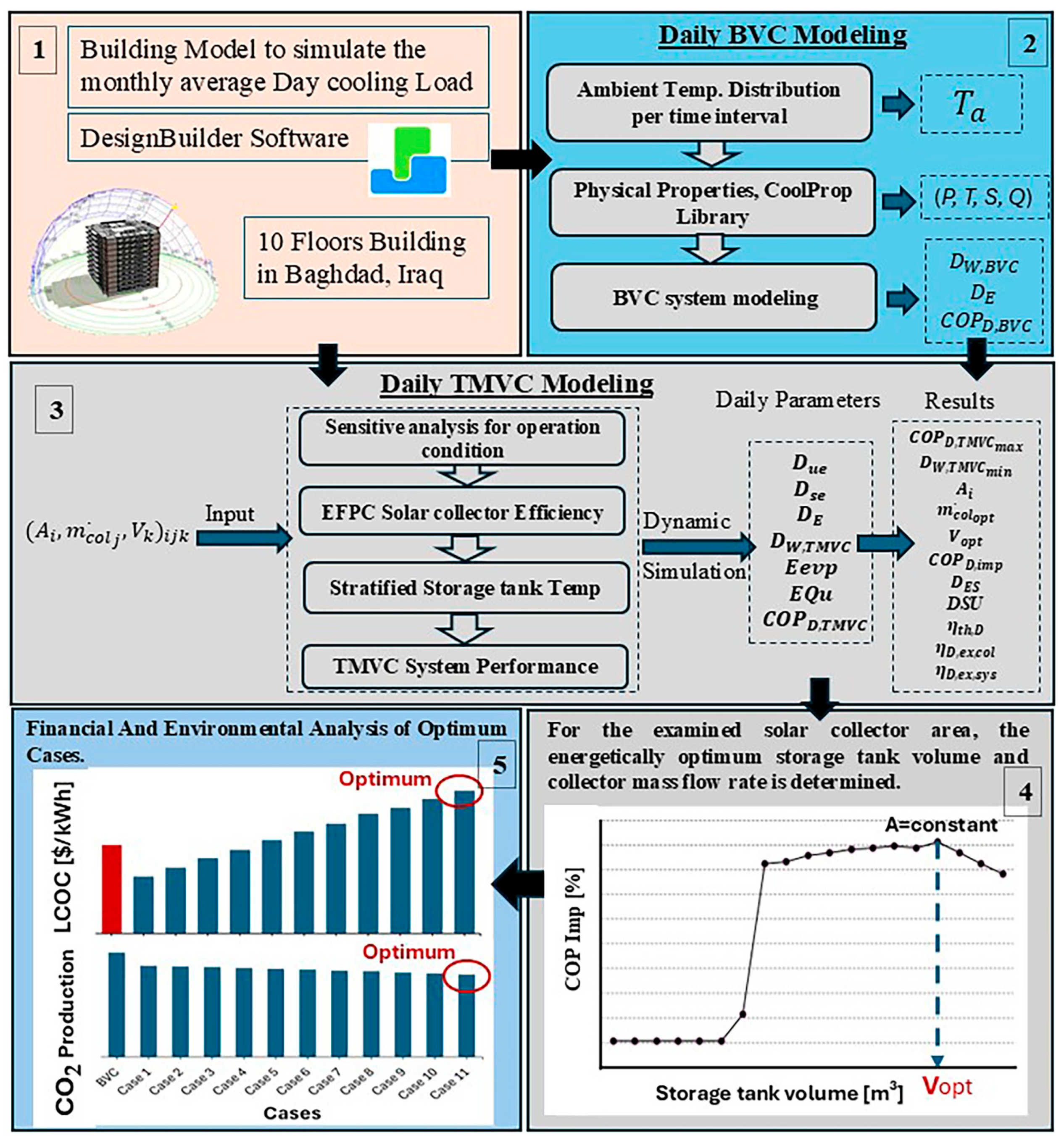
In this study, the daily performance of the solar-assisted air conditioning system was analysed and simulated to meet the building’s cooling demand. Various combinations of solar collector area, storage tank volume, and collector mass flow rate were considered. The objective is to identify the optimal storage tank volume and mass flow rate for each collector area to maximise system performance, energy savings, exergy efficiency, and the hourly utilisation of solar energy throughout the day. The results from this dynamic analysis were then used to compare the optimum configurations. Furthermore, the economic and environmental feasibility of each optimal design, including the associated CO₂ emission reductions, was evaluated.

8.1. Effect of the Collector Mass Flow Rate

The mass flow rate of the collector is a critical factor in determining the energy performance of the TMVC system. It influences both the optimal storage tank volume that maximises improvements in the coefficient of performance (COP) and energy savings compared to the basic vapour compression (BVC) system, as well as the threshold storage tank volume required to initiate the utilisation of solar energy for each collector field area.

As shown in

Table 7. Effect of collector mass flow rate on TMVC performance and tank optimisation.

	${\mathit{m}}_{\mathit{c}\mathit{o}\mathit{l}}^{.}$ = 0.01 × Ac [kg/s]			${\mathit{m}}_{\mathit{c}\mathit{o}\mathit{l}}^{.}$ = 0.02 × Ac [kg/s]			${\mathit{m}}_{\mathit{c}\mathit{o}\mathit{l}}^{.}$ = 0.03 × Ac [kg/s]			${\mathit{m}}_{\mathit{c}\mathit{o}\mathit{l}}^{.}$ = 0.04 × Ac [kg/s]
Ac [m2]	V_st (thr) [m3]	V_st (Opt) [m3]	COP_imp (max) [%]	V_st (thr) [m3]	V_st (Opt) [m3]	COP_imp (max) [%]	V_st (thr) [m3]	V_st (Opt) [m3]	COP_imp (max) [%]	V_st (thr) [m3]	V_st (Opt) [m3]	COP_imp (max) [%]
100	4	4	13.54	4	6	14.43	4	6	13.74	6	6	13.69
150	4	6	15.46	6	6	15.35	6	8	15.28	8	8	14.32
200	4	8	16.94	6	10	16.83	8	10	16.16	10	12	15.97
250	4	10	17.78	8	12	17.96	10	12	17.7	14	14	17.31
300	6	14	19.32	8	16	19.41	12	16	19.5	16	16	18.61
350	6	16	20.87	10	18	21.23	14	20	20.76	18	20	20.38
400	6	20	21.95	12	22	22.54	16	22	22.37	20	24	21.52
450	8	22	23.83	12	24	24.48	18	26	23.94	24	26	23.9
500	8	24	25.27	14	28	25.16	20	28	25.6	26	28	24.52
550	10	28	26.43	16	30	27.27	22	32	26.79	28	32	26.57
600	12	30	27.49	16	34	28.28	24	34	27.93	32	36	27.45

, as the collector mass flow rate increases from (0.01 × Ac) to (0.04 × Ac) to ensures efficient heat absorption and transfer, both the threshold and the mathematical model optimum storage tank volume show a clear upward trend, indicating that higher mass flow rates require larger storage capacities to maintain system efficiency. An increase in the mass flow rate results in more heat being transferred from the collector to the storage tank per unit of time. To effectively store this additional heat without causing temperature fluctuations, a larger tank volume is necessary to balance the energy input and output. This ensures better thermal stratification, allowing the system to maintain the required temperature gradients to achieve higher COP and energy savings.

8.2. System Optimisation

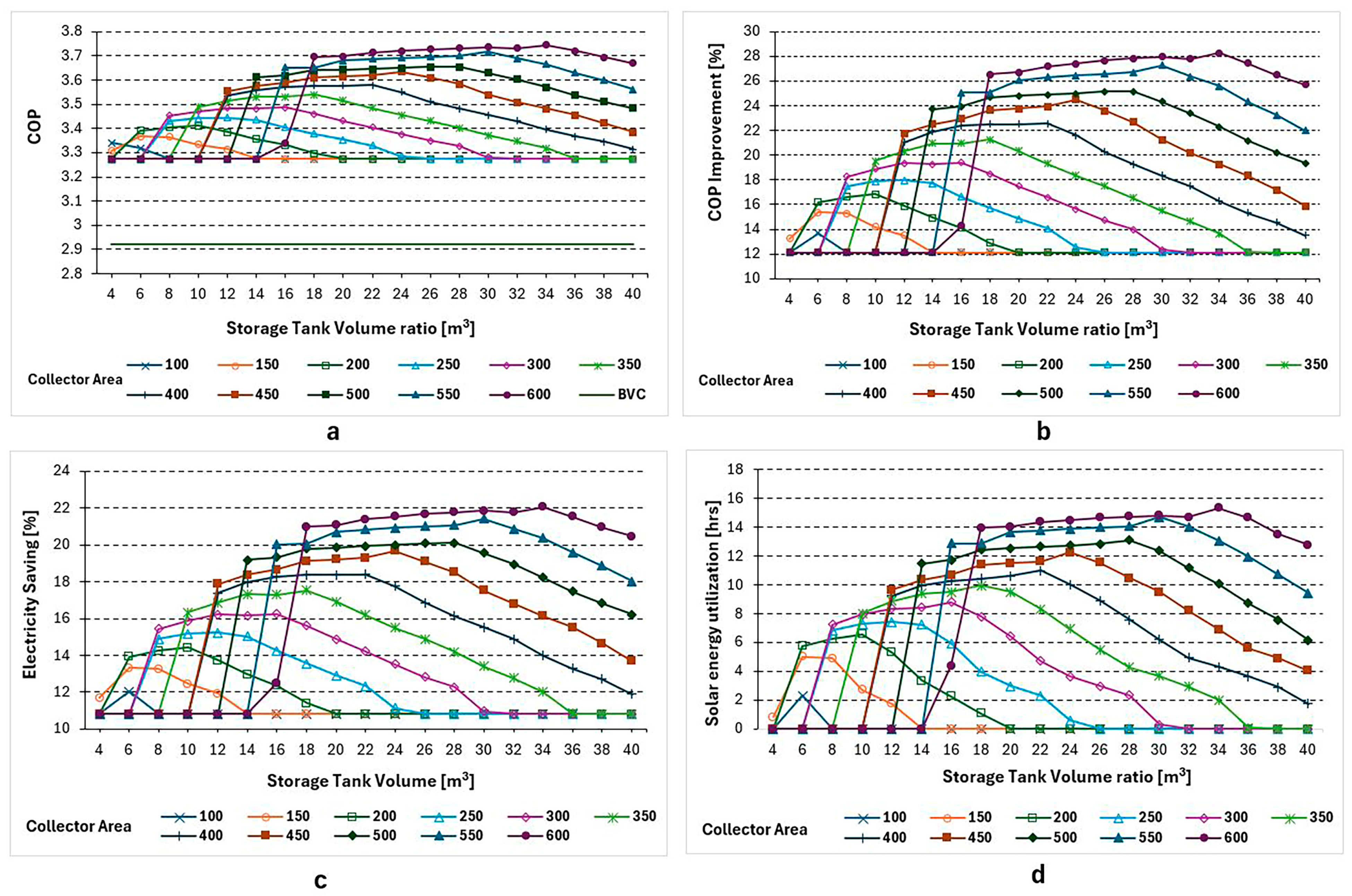
According to Figure 10a–c, each collector area has an optimal storage tank volume that maximises the daily energy performance of the TMVC system. These figures illustrate the effect of collector area and storage tank volume, at a collector mass flow rate of (0.02 × Ac), on the COP, COP improvement, and energy savings of the TMVC system compared to the BVC system.

These figures show consistent trends, as for each collector area, there is a threshold storage tank volume at which the TMVC system starts utilising solar energy for thermal compression, leading to improved COP, and energy savings. This improvement continues until it reaches an optimum storage tank volume, providing maximum COP and energy savings. Beyond this point, performance declines either because the storage tank cannot supply sufficient heat for the thermal compressor or provides heat at a lower-than-optimal rate. For smaller collector areas (100–300 m²), COP improvement and energy savings begin at a small storage tank threshold, typically below 6 m³, and reach their peak at an optimum storage tank volume of around 4–16 m³. Beyond this point, COP decreases as the effect of thermal compression fades, eventually stabilising at approximately 12.13% COP improvement and 10.8% energy savings, driven primarily by the ejector’s performance.

Conversely, for larger collector areas (400–600 m²), both the COP improvement and energy savings increase as the storage tank volume increases. The highest improvements, peaking at 28% in COP and 22% in energy savings, are seen with a 34 m³ storage tank for a 600 m² collector. These larger areas require a larger threshold storage tank size because smaller tanks cause the water temperature to rise above 170 °C, leading to boiling.

One of the key performance indicators for the solar-assisted air conditioning system is the number of hours it can utilise solar thermal energy daily across the examined configurations. As illustrated in Figure 10d, with a collector area of 400 m² and a storage tank volume exceeding 14 m³, the system can operate on solar thermal energy for more than 10 h per day. The reliance on solar energy increases significantly with larger collector areas. For instance, a configuration featuring a 600 m² collector and a storage volume of 34 m³ enables solar energy utilisation for over 15 h daily. This demonstrates that when the collector area is increased, in conjunction with an adequately sized storage tank, the daily operational hours of solar-driven thermal compression increase, effectively supplying the heat required for the thermal compressor.

Figure 11 illustrates the overall exergy efficiency of the system, highlighting the effects of collector area and storage tank volume. A clear trend is observed where exergy efficiency decreases as the collector area increases. In contrast, exergy efficiency stabilises and exhibits minimal variation with increases in storage tank volume, particularly beyond a certain threshold.

The decline in exergy efficiency with increasing collector area is attributed to the increasing exergy destruction within the system, which occurs from irreversibilities such as temperature gradients between the heat source (solar collector) and the heat sink (environment). These irreversibilities become more pronounced as the collector area increases, leading to higher thermal losses and reduced overall exergy efficiency.

Additionally, when the storage tank fails to provide the required heat to the thermal compressor, the contribution of the solar thermal system diminishes. In such cases, the system’s exergy efficiency reverts to a baseline level comparable to a vapour compression system with an ejector, as the solar thermal system’s effect fades under less favourable conditions.

Figure 12a illustrates the daily thermal efficiency of the solar collector field. The results indicate that increasing the collector area while maintaining a lower storage tank volume leads to a decrease in collector thermal efficiency. This combination results in elevated mean temperatures within the storage tank layers, which, in turn, raise the inlet temperature of the solar collector. A higher inlet temperature negatively impacts the thermal performance of the collector by increasing thermal losses due to the larger temperature difference between the collector surface and the surrounding environment. Consequently, this reduces the overall thermal efficiency of the collector.

Furthermore, for each collector area, the efficiency curve follows a characteristic trend. It begins at a threshold storage tank volume, where the collector operates with minimal efficiency. As the storage tank volume increases, the efficiency improves, benefiting from a more balanced heat storage and supply. However, as the storage tank volume becomes excessively large, the system’s thermal energy potential diminishes, and it can no longer maintain the necessary heat to supply the thermal compressor effectively. This leads to the solar thermal system eventually ceasing operation.

For example, at a collector area of 600 m² and a storage tank volume of 18 m³, the thermal efficiency is approximately 53.54%. However, with the same collector area and a larger storage tank volume of 40 m³, the efficiency improves significantly to 57.71%. This highlights the importance of balancing the collector area and storage tank volume to optimise thermal efficiency and minimise thermal losses.

Figure 12b shows the variation in collector exergy efficiency with respect to collector area and storage tank volume. It is observed that as the collector area increases, the collector exergy efficiency generally improves, particularly for smaller storage tank volumes, indicating that larger collectors utilise solar energy more effectively. Conversely, for a fixed collector area, the efficiency tends to decrease with increasing storage tank volume. This decline can be attributed to higher thermal losses or reduced efficiency in heat utilisation associated with larger tank capacities. The highest efficiencies are achieved with smaller tank volumes and larger collector areas, with a peak value of 13.3% observed for a collector area of 500 m² and a tank volume of 14 m³. This analysis highlights the importance of optimising the balance between the collector area and storage tank volume to achieve maximum exergy efficiency. Figure 13 summarises the optimal cases, along with their daily energy and exergy results.

8.3. Dynamic Behaviour of the Optimum Cases

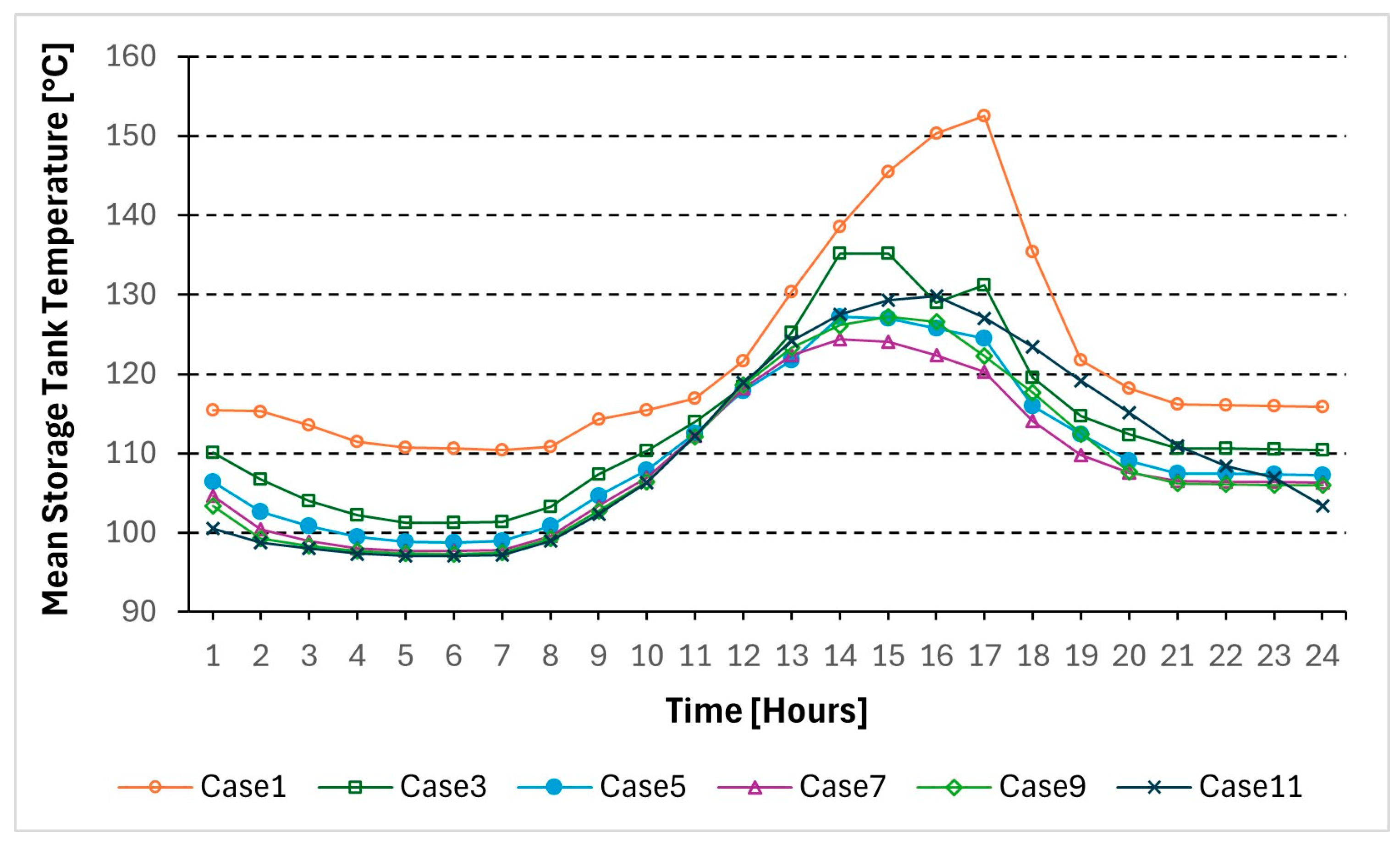
Figure 14 illustrates the mean distributed temperature inside the storage tank, providing insights into the behaviour of the TMVC system throughout the day. The temperature begins to rise around 7 a.m. as solar radiation becomes available, peaking at 3 p.m. During this period, the heat input from the solar source (charging) exceeds the heat output to the load (discharging), leading to an increase in temperature. Afterward, the temperature decreases as discharging surpasses charging, eventually reaching a steady state.

For Cases 5, 7, 9, and 11, the temperature curves exhibit smooth behaviour, indicating regular and successive charging and discharging cycles. This suggests that the heat acquired from the solar collector is sufficient to consistently supply heat from the storage tank to the load. Conversely, Case 3 exhibits fluctuating temperature profiles due to a lag between the charging and discharging processes. This lag indicates that the solar collector’s heat gain is initially insufficient to simultaneously increase the tank temperature and meet the load demand, causing fluctuations.

In case 1, while the mean temperature is higher, the smaller storage volume limits the total thermal energy that can be stored. This restriction prevents the system from sustaining a steady and sufficient heat supply to the TMVC system over time, particularly during high-demand periods or transient conditions. As a result, the temperatures in Cases 1 and 2 are higher than in the other cases, as the thermal compression process relies on adequate storage tank temperatures. These higher temperatures are accumulated over time due to delayed and irregular charging and discharging cycles.

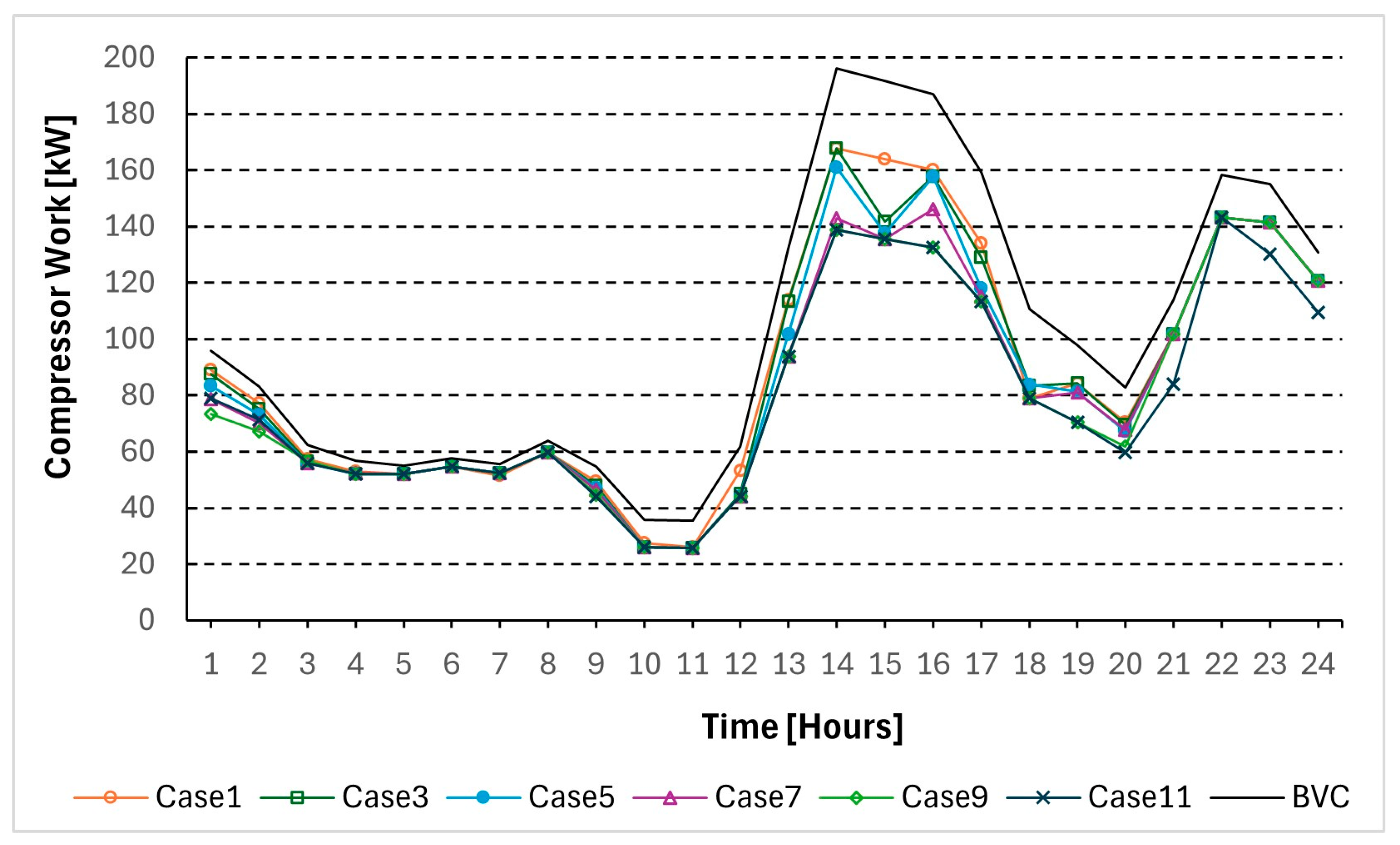
Figure 15 shows the hourly performance of the TMVC system varies across cases (Cases 1, 3, 5, 7, 9, and 11) and consistently outperforms the BVC in energy saving. During early hours (0–6 a.m.), all the TMVC cases show a lower compressor work average between (40–60 kW) compared to the BVC (50–70 kW), with Cases 9 and 11 performing slightly better due to larger storage volumes. From 7–11 h, Cases 7, 9, and 11 continue to demonstrate reduced work compared to other TMVC cases, reflecting improved thermal integration.

During peak hours (12–14), all the systems experience increased compressor work. However, TMVC cases, particularly Cases 9 and 11, maintain lower demands (140–160 kW) compared to the BVC (160–200 kW) and outperform Cases 1 and 3, which approach the BVC. In the afternoon (15–19), Cases 9 and 11 sustain moderate work levels (100–120 kW), while other TMVC cases and the BVC require more energy (130–160 kW). By evening (20–24), all TMVC cases reduce their work, with Cases 9 and 11 again showing the lowest values (60–100 kW) compared to other cases (~70–110 kW) and the BVC (70–130 kW). Overall, Cases 9 and 11 consistently achieve the best performance, emphasising the benefits of optimised storage and thermal management.

As illustrated in Figure 16, the hourly COP analysis shows that the TMVC system consistently outperforms the BVC throughout the day. TMVC cases, particularly Case 11, maintain higher COP values due to greater heat gain during the charging mode and better temperature distribution within the storage tank, with values ranging from 4.0 to 4.7, compared to the BVC (3.7–4.3) during early hours (1–6). In the afternoon (13–18), TMVC cases sustain a COP of 3.3–3.5, while the BVC drops below 2.5. By evening (19–24), TMVC cases, especially Case 11, recover with COP values rising to 3.7–4.2, surpassing the BVC (2.6–3.5). Overall, the TMVC system demonstrates improved energy efficiency, with Case 11 performing the best during high-load periods.

Figure 17 illustrates the hourly thermal efficiency of the solar collector. All the optimal cases exhibit a similar trend: efficiency increases after sunrise as solar radiation becomes available, peaks around noon, and then gradually declines toward sunset. However, Case 11 shows a slight deviation to the left after noon. This deviation occurs due to the increasing temperature distribution, which raises the inlet water temperature to the collector, thereby reducing the collector’s efficiency.

Figure 18 shows the monthly average daily electricity consumption for all the months, comparing the BVC with the TMVC optimal case. Electricity consumption is highest in July and August due to higher mean ambient temperatures, which result in a lower COP. The BVC consistently demonstrates the highest compressor work, reflecting greater daily energy consumption compared to the TMVC cases. The integration of a thermal compressor in the TMVC cases demonstrates improved energy efficiency, particularly during high-load months.

8.4. Economic Analysis

An economic analysis was conducted for the optimal cases, comparing them to the basic vapour compression cycle (BVC) using the levelised cost of cooling (LCOC), including the total environmental penalty cost savings accrued over the system’s lifetime. This financial evaluation considers all summer months (April to October) to determine the electricity savings achieved through the implementation of the TMVC system.

One of the primary challenges impacting the economic feasibility of renewable energy projects in Iraq, particularly those targeting reductions in electricity consumption, is the government’s subsidy for residential electricity prices, which can be as low as $0.015 per kWh. This substantial subsidy makes it difficult for competing projects to achieve economic viability. To address this, the present study assumes an average electricity price of $0.15 per kWh for analysis.

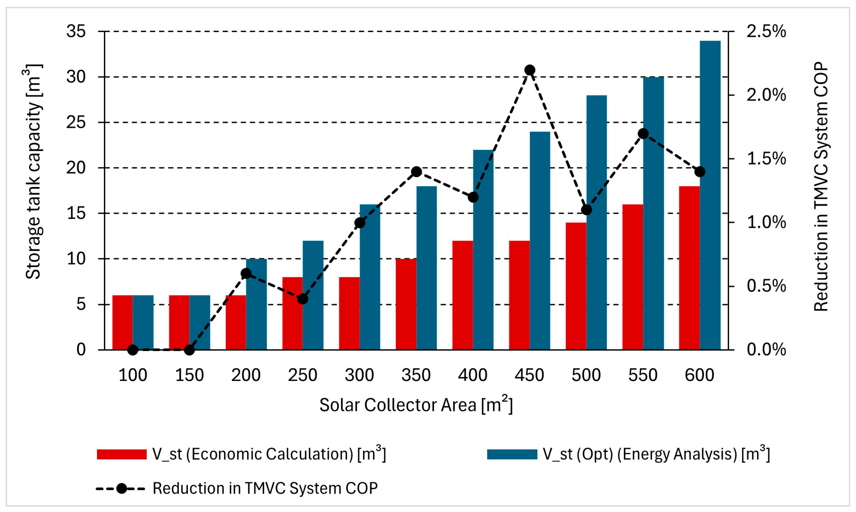
In order to reduce the capital cost and achieve acceptable economic results, a sensitivity analysis was conducted to evaluate the impact of reducing the storage tank volume per cubic meter on the TMVC system’s COP. The storage tank is the most expensive component of the system, making it a key focus for cost optimisation. The results, presented in Figure 19, identify the optimum storage tank size for each case and count the percentage change in COP when the storage tank volume is reduced to an acceptable level that maintains the internal temperature within acceptable limits.

Figure 20 illustrates the levelised cost of cooling (LCOC) for various configurations of the TMVC system, compared to the baseline vapour compression cycle (BVC) as a reference. As the configurations progress from Case 1 to Case 11, the LCOC generally increases, indicating a rise in the cost of cooling. In configurations with smaller collector areas and storage tank volumes (Cases 1 to 3), the TMVC system achieves a noticeable cost reduction compared to the BVC. Notably, Case 4 achieves an LCOC of 0.053 $/kWh, closely matching the cost of the BVC. Beyond this point, the LCOC continues to rise, with Case 11 exhibiting the highest cost at $0.063/kWh, representing a 16% increase over the baseline.

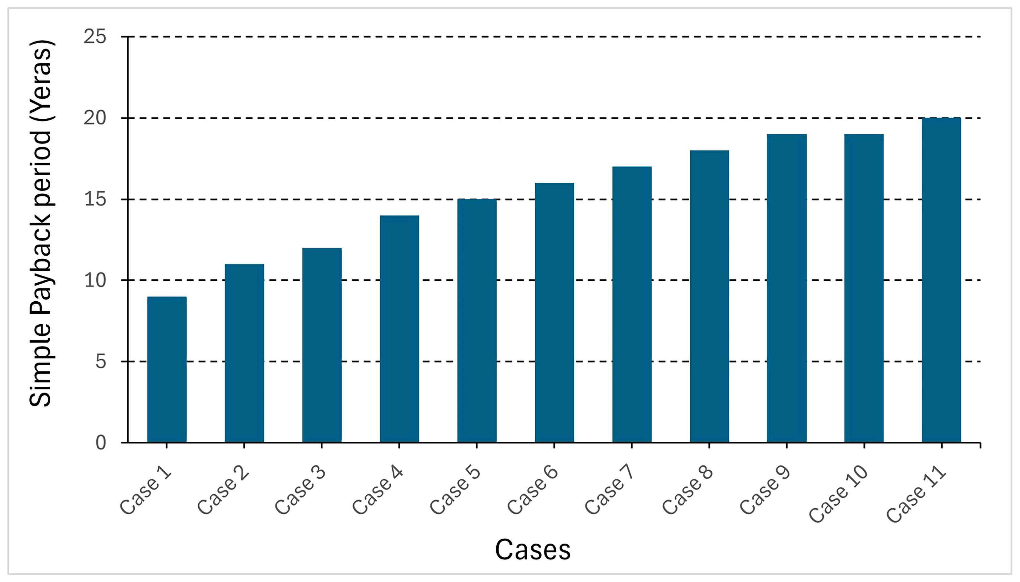
Figure 21 illustrates the simple payback period (SPBP) for the various TMVC system configurations. A clear trend is observed: as the collector area and storage tank volume increase across the cases, the SPBP correspondingly rises due to higher capital investment.

Case 1 offers the shortest payback period of 9 years, attributed to its relatively low system cost, while Case 11 exhibits the longest payback period of 20 years despite achieving the highest energy savings and environmental benefits. This highlights the economic-performance trade-off, where configurations with greater sustainability gains (e.g., Case 11) require a longer investment recovery period, whereas lower-cost systems (e.g., Case 1) yield faster returns but more modest energy and emissions reductions.

8.5. Environmental Analysis

The emissions comparison analysed the CO₂ generated from electricity consumption required to operate the BVC and TMVC systems during the summer season, focusing on the reduction achieved by each optimal case. As illustrated in Figure 22, the TMVC system consistently results in lower CO₂ emissions compared to the BVC system. Among the cases, Case 11 stands out as the optimal configuration for emissions reduction, producing 294 tons of CO₂ over the summer, achieving a 21% reduction relative to the BVC system, highlighting its potential for environmental benefits.

8.6. Comprehensive Evaluation Index

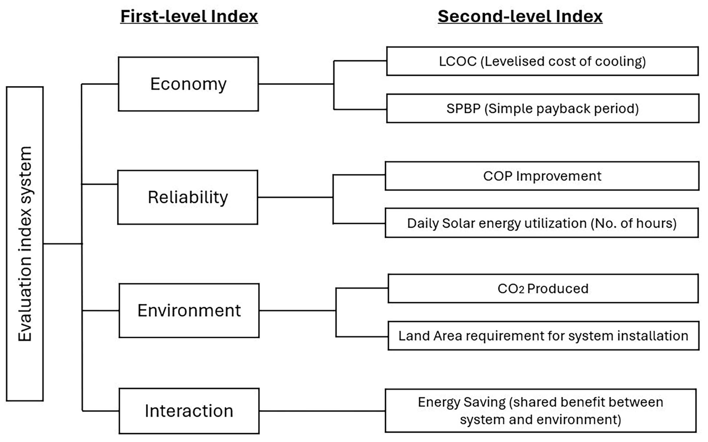
In this study, a comprehensive evaluation index method was implemented to rank 11 design cases of a TMVC system based on multiple performance indicators implemented as shown in Figure 23, The approach is adapted from Liu et al., (2022) [43], who proposed a hybrid AHP–entropy method for smart grid evaluation. To simplify and tailor the method for TMVC systems, a two-stage index structure is constructed. The first-level indicators include economy, reliability, environmental impact, and interaction, while the second-level indicators consist of COP improvement, energy saving, solar energy utilization hours, levelised cost of cooling (LCOC), simple payback period (SPBP), CO₂ produced, and required land area for solar equipment installation.

The evaluation framework integrates min–max normalisation and the analytic hierarchy process (AHP) to ensure both comparability and rational weighting of diverse criteria.

To ensure comparability across indicators, different units, and scales, min–max normalisation is applied. For benefit indicators like COP improvement, energy savings, and daily solar hours utilisation (DSU), where higher values are preferable, normalisation is performed using the following:

$$X^{\prime }={\displaystyle \frac{X_j-X_{min}}{X_{max}-X_{min}}}$$

(27)

For cost indicators (e.g., LCOC, SPBP, CO₂ emissions, and land area), where lower values are preferable, normalisation is inverted as follows:

$$X^{\prime }={\displaystyle \frac{X_{max}-{\mathrm{X}}_j}{X_{max}-X_{min}}}$$

(28)

This process transforms all values into a [0, 1] range, where 1 denotes the best performance.

The weighting of indicators is determined using the analytic hierarchy process (AHP), a structured decision-making technique that converts qualitative judgments into quantitative weights. Pairwise comparisons are performed between each pair of indicators to construct a judgment matrix. Construct the judgment matrix w_i, and its expression is denoted as follows:

$$w=\left[\begin{array}{cccccccc}& {COP}_{imp}& ES& DSU& LCOC& SPBP& {CO}_2& A_{land}\\ {COP}_{imp}& 1& 0.75& 1& 1& 1.5& 0.75& 3\\ ES& 1.333& 1& 1.333& 1.333& 2& 1& 4\\ DSU& 1& 0.75& 1& 1& 1.5& 0.75& 3\\ LCOC& 1& 0.75& 1& 1& 1.5& 0.75& 3\\ SPBP& 0.666& 0.5& 0.666& 0.666& 1& 0.5& 2\\ {CO}_2& 1.333& 1& 1.333& 1.333& 2& 1& 4\\ A_{land}& 0.333& 0.25& 0.333& 0.333& 0.5& 0.25& 1\end{array}\right]$$

Each column of the matrix was normalised by dividing each entry by the sum of its column. The weight vector for each indicator was then derived by taking the average of the normalised rows. The resulting weight of COP improvement, ES, DSU, LCOC, SPBP, CO₂ production, and required land area for solar equipment installation are 0.15, 0.2, 0.15, 0.15, 0.1, 0.2, and 0.05, respectively. These weights align with Iraq’s national priorities, which promote sustainable investment and environmental protection. The relatively low weight assigned to the payback period reflects Iraq’s capacity to support long-term infrastructure development.

Using these AHP-derived weights w_i, the final comprehensive evaluation score for each TMVC system configuration is computed as a weighted sum of normalised indicator values, as follows:

$$S_i={\sum }_1^7{w}_i·X_{ji}$$

(29)

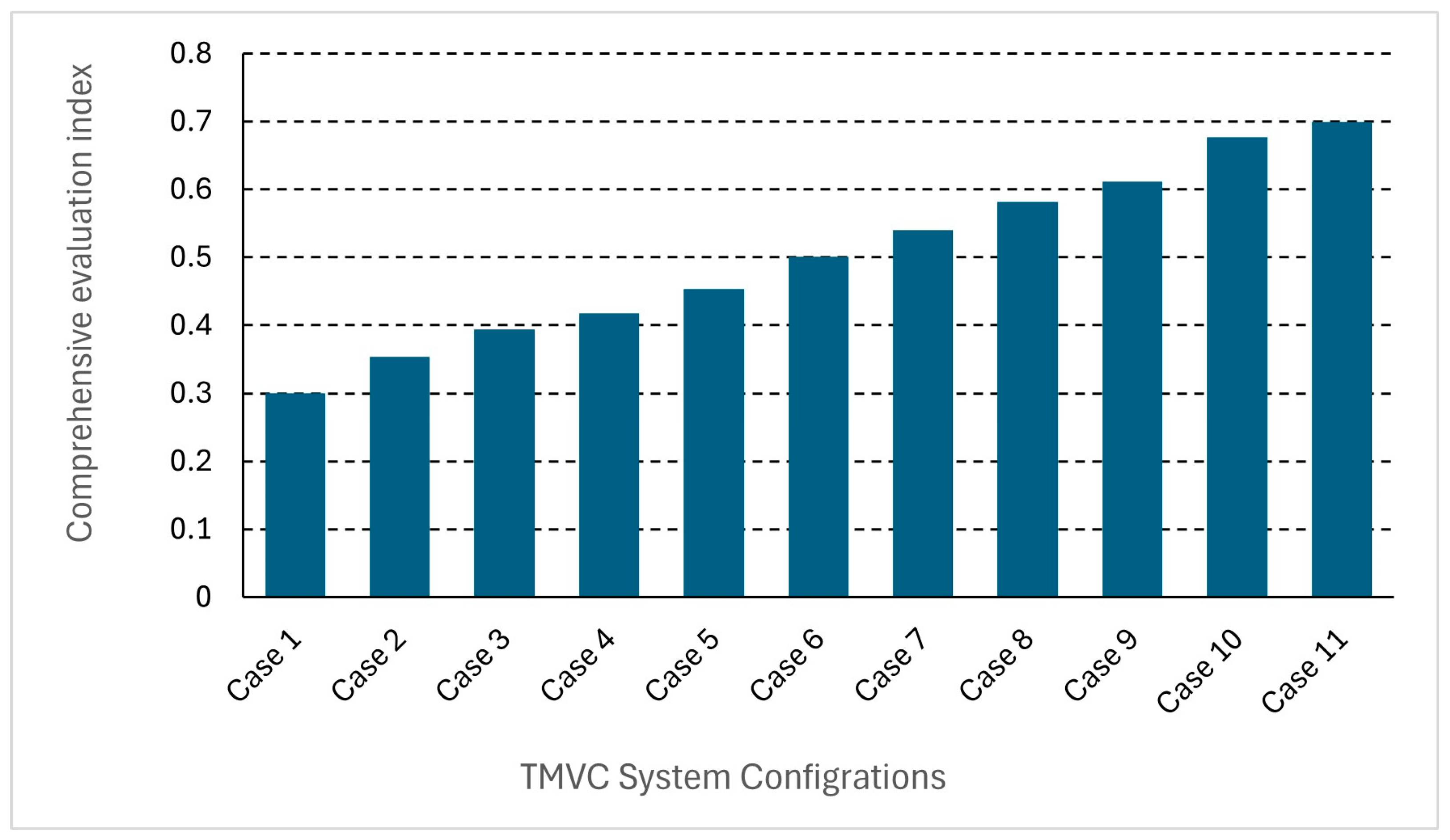
The final results, as shown in Figure 24, revealed that Case 11 achieved the highest composite score (0.7), indicating the most balanced performance across technical, economic, and environmental criteria. This methodology provides a robust, transparent, and rational basis for multi-criteria decision-making in sustainable cooling system design.

8.7. Comparison of Economic Index TMVC with Other Systems

According to reference [11], which presents an economic analysis of various solar-assisted cooling systems, including solar thermal absorption (SABC), solar thermal adsorption (SADC), PV-assisted vapour compression (PV-BVC), PVT-assisted absorption (PVT-ABC), and PVT-assisted adsorption (PVT-ADC). The levelised cost of cooling (LCOC) was used as a key indicator to assess their performance across different global cities. In this study, the LCOC of the TMVC case is compared with the average LCOC of each of these solar-assisted systems. As illustrated in Figure 25, TMVC remains economically competitive among other solar cooling technologies and offers a practical solution to reduce electricity consumption in hot climate regions without replacing the existing cooling system, requiring only the integration of solar thermal components.

9. Conclusions

This study evaluated the performance of a solar-assisted thermo-mechanical vapour compression (TMVC) cooling system for multi-story residential buildings in hot climate regions. A comprehensive 4E (energy, exergy, economic, environmental) analysis was conducted using a hybrid simulation approach, where building performance parameters were obtained through DesignBuilder, and system-level simulations and optimisation were performed using MATLAB^® R2023b, incorporating real hourly climate data for Baghdad, Iraq.

Eleven system configurations were examined by varying the solar collector area, thermal storage tank volume, and collector mass flow rate. The results showed that increasing the solar field and storage capacity generally enhanced energy performance but also increased system costs. Among the analysed configurations, Case 11 featuring a 600 m² solar collector and 34 m³ storage tank with a collector mass flow rate of 0.02 kg/s was identified as the optimal solution based on a comprehensive evaluation index. It achieved a 28.28% increase in COP, a 22.05% reduction in energy consumption, a 21% reduction in CO₂ emissions, and 15.3 h of average daily solar-assisted operation during summer conditions; however, the daily exergy efficiency drops to below 15% due to irreversibilities such as temperature gradients between the solar collector and the environment, making it a less favourable performance index for the TMVC system. Economically, this case resulted in a simple payback period (SPBP) of 20 years and a levelised cost of cooling (LCOC) of $0.066/kWh, which, despite being higher than the baseline system by 16%, aligns with the long-term sustainability targets and infrastructure investment priorities outlined in Iraq’s national housing and energy policies.

The key advantages of the TMVC system over the conventional vapour compression cycle include shifting part of the compression process to solar thermal input, thereby reducing the mechanical compressor workload. This leads to lower energy consumption and reduces environmental impact, supporting the adoption of sustainable cooling technologies. Additionally, the system offers a scalable solution suitable for multi-story residential buildings or district cooling applications in hot climate zones. Further experimental work is required to evaluate the system’s real-world performance and operational reliability.