A Data Imputation Approach for Missing Power Consumption Measurements in Water-Cooled Centrifugal Chillers

Abstract

In the process of collecting operational data for the performance analysis of water-cooled centrifugal chillers, missing values are inevitable due to various factors such as sensor errors, data transmission failures, and failure of the measurement system. When a substantial amount of missing data is present, the reliability of data analysis decreases, leading to potential distortions in the results. To address this issue, it is necessary to either minimize missing occurrences by utilizing high-precision measurement equipment or apply reliable imputation techniques to compensate for missing values. This study focuses on two water-cooled turbo chillers installed in Tower A, Seoul, collecting a total of 118,464 data points over 3 years and 4 months. The dataset includes chilled water inlet and outlet temperatures ($T_1$ and $T_2$) and flow rate (${\dot{V}}_1$) and cooling water inlet and outlet temperatures ($T_3$ and $T_4$) and flow rate (${\dot{V}}_3$), as well as chiller power consumption (${\dot{W}}_c$). To evaluate the performance of various imputation techniques, we introduced missing values at a rate of 10–30% under the assumption of a missing-at-random (MAR) mechanism. Seven different imputation methods—mean, median, linear interpolation, multiple imputation, simple random imputation, k-nearest neighbors (KNN), and the dynamically clustered KNN (DC-KNN)—were applied, and their imputation performance was validated using MAPE and CVRMSE metrics. The DC-KNN method, developed in this study, improves upon conventional KNN imputation by integrating clustering and dynamic weighting mechanisms. The results indicate that DC-KNN achieved the highest predictive performance, with MAPE ranging from 9.74% to 10.30% and CVRMSE ranging from 12.19% to 13.43%. Finally, for the missing data recorded in July 2023, we applied the most effective DC-KNN method to generate imputed values that reflect the characteristics of the studied site, which employs an ice thermal energy storage system.

1. Introduction

1.1. Research Background and Objectives

Water-cooled chillers play a crucial role in maintaining stable indoor environments in large-scale cooling systems. They primarily handle the cooling demands of large buildings and, as a result, account for a significant proportion of total energy consumption [1]. In recent years, improving the efficiency of chillers has become a critical challenge, particularly in response to climate change. Notably, the summers of 2023 and 2024 experienced record-breaking heat waves, along with abnormal autumnal high temperatures, leading to a sharp increase in cooling demand. Consequently, it has become essential to manage chillers efficiently to maintain a stable indoor climate while simultaneously reducing energy consumption [2]. The control of the chilled water outlet temperature in water-cooled chillers directly influences the coefficient of performance (COP) and overall power consumption. This indicates that optimizing operational conditions can significantly reduce building energy usage [3]. To assess this relationship, it is necessary to collect and analyze data over an extended period, including chilled water and cooling water temperatures, flow rates, and power consumption. However, collected data often contain missing values due to sensor failures, data transmission errors, or environmental factors. If missing values occur in sensor data during cooling operations, the predictive accuracy of analytical models decreases. Missing values can introduce errors in model training or reduce the dataset size when removed, ultimately leading to a decline in model performance [4]. Thus, an effective strategy for imputing missing data is crucial to ensure data quality. This study applies and evaluates various imputation techniques to enhance the quality of chiller operational data. A total of 118,464 real-world data points were subjected to a missing-at-random (MAR) mechanism. The missing data were then imputed using seven different techniques, and their performance was assessed. Finally, the most effective imputation method was applied to replace missing values in the dataset for July 2023.

1.2. Limitations of Previous Studies

Previous studies have utilized a variety of statistical techniques and machine learning algorithms for missing data imputation. However, several recurring limitations have been observed:

A.

Many prior works applied a single imputation method without conducting a thorough analysis of the missing data mechanism, such as missing completely at random (MCAR) or missing at random (MAR). As a result, the selected methods often failed to reflect the true nature of the data, leading to reduced imputation quality [5];

B.

In high-dimensional and dynamically changing environments, such as time-series sensor data, traditional studies have predominantly relied on simplistic statistical approaches such as mean substitution, linear interpolation, or regression-based imputation. While computationally efficient, these methods are limited in their ability to capture complex temporal patterns and inter-cluster heterogeneity [6];

C.

Conventional data-driven methods such as k-nearest neighbors (KNNs) rely on fixed-distance similarity measures, which fail to consider the existence of clustered structures or local variations. As a result, their performance tends to degrade under varying operational conditions or device-specific patterns [7];

D.

There is a lack of advanced imputation techniques tailored to real-world sensor-based environments. Particularly in physical systems such as water-cooled chillers, various types of missing data may occur due to environmental disturbances, sensor malfunctions, or communication failures. However, case studies addressing such practical scenarios remain limited [8].

To overcome these challenges, this study proposes a novel algorithm—dynamically clustered k-nearest neighbors (DC-KNNs)—which reflects inherent data clusters through unsupervised clustering and applies dynamic weighting schemes within each cluster. By improving on the limitations of conventional KNNs, the proposed method provides more precise imputations that respect the structural complexity of time-series sensor data. This advancement not only enhances imputation precision but also significantly contributes to more reliable and accurate forecasting in intelligent energy systems [9].

1.3. Research Objectives and Scope

This study aims to identify missing values within a dataset consisting of 118,464 operational records from two water-cooled turbo chillers over a three-year period. The research systematically compares and analyzes various statistical imputation techniques to determine the most effective method. Missing values were imputed using mean imputation, median imputation, linear interpolation, multiple imputation, simple random imputation, and KNN imputation. The most effective approach was then further enhanced by proposing a DC-KNN imputation method. The DC-KNN method enhances traditional KNN imputation by addressing two core limitations: ① equal weighting of variables regardless of their predictive power and ② blind selection of neighbors solely based on global distance metrics without considering local data structures.

A.

Variable-specific importance weighting

Unlike conventional KNNs, where all variables contribute equally to the distance computation, the DC-KNN method assigns a tailored weight to each variable based on its statistical importance in predicting the target variable. For instance, in the context of chiller operation data, features such as flow rate or evaporator outlet temperature may exhibit stronger correlations with the missing variable than others (e.g., ambient temperature). These weights are either of the following:

• Computed via correlation coefficients, mutual information, or domain-specific feature ranking;
• Integrated directly into the distance function, allowing more relevant variables to exert greater influence.

This mechanism improves sensitivity to domain-relevant features, enhancing imputation precision in complex physical systems like heating, ventilation, and air conditioning (HVAC) operations.

B.

Cluster-based neighbor selection

The standard KNN method selects the k-nearest neighbors globally, which risks drawing in contextually dissimilar instances, especially in heterogeneous datasets with multiple operational modes or patterns.

The DC-KNN method first performs unsupervised clustering based on data similarity profiles and then restricts neighbor selection to the cluster that the instance belongs to. This allows the method to achieve the following:

• Respect local data topology;
• Reduce contamination from out-of-distribution points;
• Preserve the semantic integrity of imputed values.

For example, a chiller operating under partial load conditions will seek imputation references only from similar partial-load samples rather than from full-load or standby modes.

1.4. Key Contributions of This Study

This study proposes the DC-KNN imputation method to overcome the limitations of existing techniques and enhance the reliability of chiller operation data. By improving the accuracy of COP (Coefficient of Performance) analysis, this method is expected to contribute to improving data quality within Building Energy Management Systems (BEMSs). The key contributions of this study are as follows:

A.

Introduction of a novel approach to address missing data in chiller operation data:

• Analyzes the limitations of commonly used imputation methods, such as mean imputation, median imputation, linear interpolation, and KNN imputation;
• Develops a new DC-KNN imputation method that improves upon conventional KNNs by incorporating clustering-based filtering and dynamic weighting, leading to more precise missing data imputation.

B.

Demonstration of practical applicability using real operational data:

• The dataset consists of 118,464 chiller sensor records collected over three years in a real-world operational environment, ensuring high practical applicability;
• The analysis is conducted based on long-term observed data, enhancing the reliability of the imputed results by utilizing an extensive dataset.

C.

Analysis of the optimal combination of missing data rates and imputation techniques:

• This study compares and analyzes various missing data imputation techniques to identify the optimal imputation method based on different missing rates (10%, 20%, and 30%). This research provides valuable insights into data-driven chiller performance optimization and offers a robust guideline for handling missing data in HVAC system analysis.

2. Theoretical Review

2.1. Outlier Detection

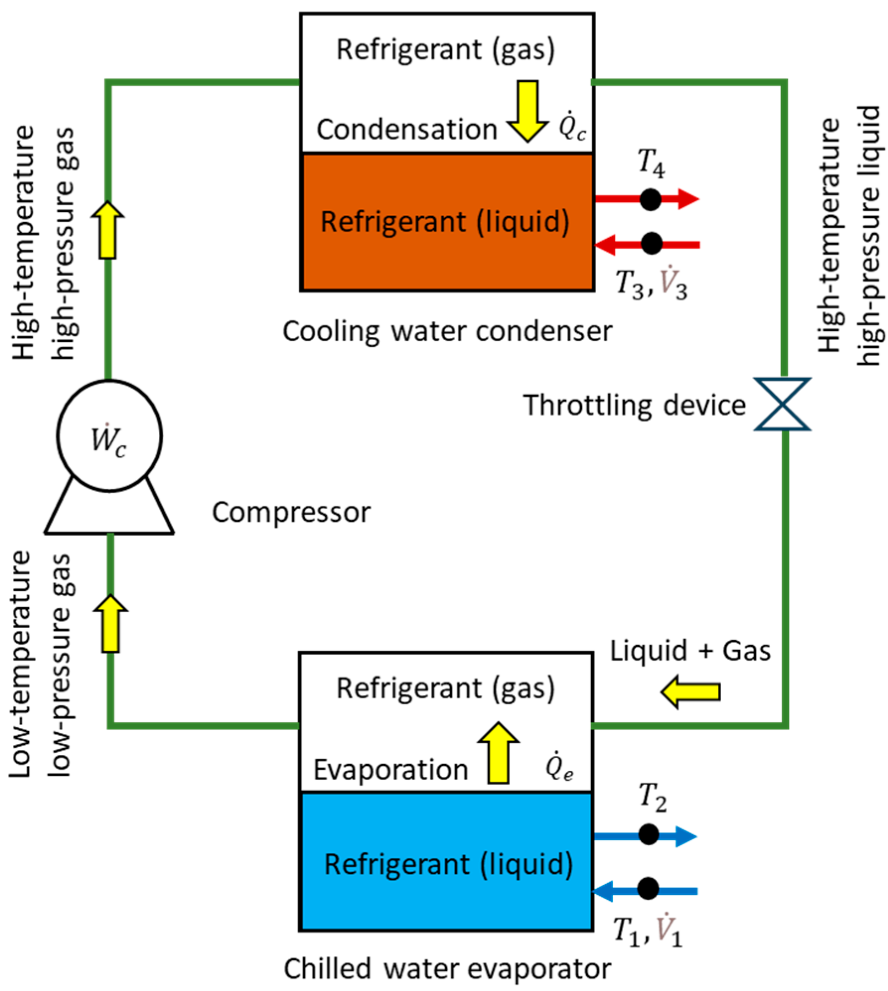
2.1.1. Thermodynamic Characteristics of Chillers

The thermodynamic characteristics of water-cooled chillers are defined by the interaction between heat and work within the refrigeration cycle. Heat and work represent the two fundamental forms of energy transfer in thermodynamics, each governed by distinct principles and mechanisms. Heat transfer occurs due to temperature differences, whereas work is the transfer of energy resulting from a force applied over a distance. Unlike stored energy, such as internal energy, heat and work exist only when energy moves across system boundaries. This distinction highlights the transient nature of heat and work, where energy can enter or leave a system in these forms but cannot be stored as heat or work itself.

The relationship between heat and work is formalized by the first law of thermodynamics, which states that energy cannot be created or destroyed but can only be converted from one form to another. This principle plays a crucial role in refrigeration systems, where mechanical work applied by the compressor enables heat transfer from a low-temperature heat source (evaporator) to a high-temperature heat sink (condenser). During this process, the refrigerant absorbs heat in the evaporator, requiring work input to circulate the refrigerant, and subsequently releases heat in the condenser.

One of the key concepts in the interaction between heat and work is entropy. While heat transfer always involves entropy transfer, work transfer does not. This distinction indicates that heat contains a certain level of disorder, whereas work represents a more structured form of energy transfer. Consequently, the efficiency of a refrigeration cycle depends not only on the amount of energy transferred but also on the mode of transfer and its impact on system entropy.

Understanding the interaction between heat and work in practical refrigeration applications is essential for optimizing system performance. The refrigeration cycle consists of four primary processes: evaporation, compression, condensation, and expansion. These processes are maintained through a controlled interaction of heat absorption, mechanical work input, and heat release. Effective management of these energy transfers improves chiller efficiency, reduces energy consumption, and ensures optimal cooling performance.

The refrigerant absorbs heat in the evaporator, releases heat in the condenser, and consumes energy in the compressor to circulate throughout the system. In the evaporator, the refrigerant utilizes the temperature difference between the inlet and outlet chilled water to achieve cooling, thereby providing a cooling effect. The system’s components, operating mechanisms, and thermal storage processes are illustrated in Figure 1. The energy transfer process in the chiller is expressed by the following heat transfer equation [10]:

$$\dot{Q}=\rho \dot{V}c∆T$$

(1)

$${\dot{Q}}_e={\rho }_b{\dot{V}}_1{c}_b(T_1-T_2)$$

(2)

$${\dot{Q}}_c={\rho }_w{\dot{V}}_3{c}_w(T_4-T_3)$$

(3)

2.1.2. Energy Balance Error (EB)

In this study, reliable data were selected based on the first law of thermodynamics by utilizing the energy balance error (EB). ${\dot{Q}}_e$ and ${\dot{Q}}_c$ were calculated to assess whether the data satisfied the first law of thermodynamics. Data with an EB within ±5% were considered reliable, whereas data outside this range were likely affected by sensor measurement errors, refrigerant flow fluctuations, or partial load operations [11,12].

As a result, only data within an EB of ±5% were deemed reliable in this study. This approach ensured data quality, significantly enhancing the model’s reliability and predictive accuracy. The EB is calculated as follows: In Equation (4), the numerator $\left({\dot{Q}}_e+{\dot{W}}_c\right)-{\dot{Q}}_c$ represents the deviation in energy balance and dividing this by ${\dot{Q}}_c$ yields the relative error (ratio). Consequently, the EB value is a dimensionless quantity, allowing the system’s balance to be expressed as a percentage (%):

$$\mathrm{E}\mathrm{B}(\pm 5\%)={\displaystyle \frac{\left({\dot{Q}}_e+{\dot{W}}_c\right)-{\dot{Q}}_c}{{\dot{Q}}_c}}$$

(4)

2.1.3. Coefficient of Performance (COP)

COP is an indicator of how efficiently a chiller operates. Since the primary objective of a chiller is to minimize the energy consumed in the process of heat removal or transfer, the coefficient of performance serves as a critical metric for evaluating the energy efficiency of a chiller system. COP is expressed by the following equation [13]:

$$\mathrm{C}\mathrm{O}\mathrm{P}={\displaystyle \frac{{\dot{Q}}_e}{{\dot{W}}_c}}$$

(5)

2.2. Imputation Methods

Statistical methods for missing data imputation have been widely used for an extended period due to their computational simplicity and ease of application. In this study, various representative statistical imputation techniques were compared and analyzed to determine the most suitable method.

2.2.1. Mean Imputation

Mean imputation replaces missing values with the mean of the corresponding variable, effectively preserving the overall average trend of the dataset. However, this method is highly sensitive to outliers and may introduce distortions in the data distribution. Despite these limitations, mean imputation is computationally simple and widely used, particularly in the initial stages of data preprocessing [14,15]:

$$y_{\mathrm{i}\mathrm{m}\mathrm{p}\mathrm{u}\mathrm{t}\mathrm{e}\mathrm{d}}={\displaystyle \frac{1}{N}}\sum _{i=1}^N{y}_i$$

(6)

2.2.2. Median Imputation

Median imputation replaces missing values with the median of the corresponding variable, making it suitable for mitigating the influence of non-normal distributions and outliers. This method provides stable imputation results, especially for datasets with extreme values. The median is determined by sorting the data in ascending order and selecting the central value, effectively minimizing the impact of outliers when imputing missing data [16,17]:

$$y_{\mathrm{i}\mathrm{m}\mathrm{p}\mathrm{u}\mathrm{t}\mathrm{e}\mathrm{d}}=Median\left(y\right)$$

(7)

2.2.3. Linear Interpolation

Linear interpolation estimates missing values in time-series data by interpolating between adjacent values based on a linear relationship. This method is useful for maintaining the natural trend of the data and offers computational simplicity and high interpretability. However, it has limitations in capturing abrupt fluctuations or nonlinear relationships within the data [18,19]:

$$y_{\mathrm{i}\mathrm{m}\mathrm{p}\mathrm{u}\mathrm{t}\mathrm{e}\mathrm{d}}=y_{i-1}+(y_{i+1}-y_{i-1}){\displaystyle \frac{t_i-t_{i-1}}{t_{i+1}-t_{i-1}}}$$

(8)

2.2.4. Multiple Imputation

Multiple imputation replaces missing values multiple times and calculates the final imputed value as the average of these imputed results, thereby reflecting the uncertainty associated with missing data. This method provides reliable results and is particularly effective for handling missing-at-random (MAR) data [20,21]:

$$y_{\mathrm{i}\mathrm{m}\mathrm{p}\mathrm{u}\mathrm{t}\mathrm{e}\mathrm{d}}={\displaystyle \frac{1}{m}}\sum _{j=1}^m{Y}_{i,j}$$

(9)

2.2.5. Simple Random Imputation

Simple random imputation replaces missing values with randomly generated values based on the existing distribution of the variable. While this approach aims to maintain the probabilistic characteristics of the original data, it has the drawback of introducing significant variability in the imputed results [22,23]:

$$y_{\mathrm{i}\mathrm{m}\mathrm{p}\mathrm{u}\mathrm{t}\mathrm{e}\mathrm{d}}=y_{obs}+ϵ$$

(10)

2.2.6. KNN Imputation

K-nearest neighbor (KNN) imputation replaces missing values with either the mean or median of the K most similar neighboring data points. This method is particularly useful for datasets containing highly correlated variables, as it can capture complex multidimensional relationships while preserving data structure and patterns. However, KNN imputation is computationally expensive, and processing time increases as the dataset size grows [24,25]:

$$y_{\mathrm{i}\mathrm{m}\mathrm{p}\mathrm{u}\mathrm{t}\mathrm{e}\mathrm{d}}={\displaystyle \frac{1}{K}}\sum _{i=1}^K{y}_{\mathrm{n}\mathrm{e}\mathrm{i}\mathrm{g}\mathrm{h}\mathrm{b}\mathrm{o}\mathrm{r}}$$

(11)

2.2.7. Euclidean Distance

Euclidean distance is suitable for continuous data, assuming that closer data points exhibit higher similarity. This method calculates the straight-line distance between two points. Given two data points, $x$ and $y$, the Euclidean distance is defined as follows [26]:

$$d_{\mathrm{E}\mathrm{u}\mathrm{c}}\left(y_i,y_j\right)=\sqrt{\sum _{i=1}^n{\left(y_{ik}-y_{jk}\right)}^2}$$

(12)

2.2.8. Cosine Similarity

Cosine similarity focuses on the direction rather than the magnitude of the data and is particularly effective for normalized datasets. This method calculates similarity by measuring the angle between two vectors, with values ranging from −1 to 1. Cosine similarity is defined as follows [27]:

$$S_{\mathrm{C}\mathrm{O}\mathrm{S}}(y_i,y_j)={\displaystyle \frac{y_i·y_j}{\left|\right|y_i\left|\right| \left|\right|y_j\left|\right|}}$$

(13)

2.2.9. DC-KNN Imputation

The DC-KNN imputation method is an enhanced imputation approach developed in this study. It first clusters data with similar patterns to the missing-value-containing records using the K-means algorithm and then applies KNNs within each cluster to perform imputation. This method improves upon the limitations of conventional KNN imputation, which relies solely on distance-based neighbor selection, by integrating clustering-based filtering and variable-specific dynamic weighting into an extended KNN approach. Initially, missing-value-containing records are grouped into clusters with similar patterns based on operational variables such as chilled water temperatures and flow rates. Among various clustering techniques, K-means is explicitly employed in this study due to its suitability for partitioning chiller operation data by temperature and load range. Although other methods, such as DBSCAN, are referenced in the literature for noise removal in sensor data with abrupt variations [14,28], only K-means is used in the implementation of DC-KNNs for this research.

K-means is a distance-based unsupervised clustering algorithm that partitions the dataset into K clusters by minimizing the within-cluster sum of squared distances (WCSS). It iteratively assigns each data point to the nearest cluster centroid and updates the centroids until convergence. This approach is particularly well-suited for time-series sensor data with continuous, normalized variables—such as temperature and flow rate—where Euclidean distance is a meaningful similarity metric.

On the other hand, density-based clustering techniques, like DBSCAN, are advantageous for handling nonlinear cluster shapes or identifying noise points in unstructured data. However, they are less suitable for structured operational datasets, especially in scenarios where a fixed number of interpretable clusters is required. DBSCAN’s sensitivity to parameter settings (e.g., epsilon and minimum samples) and lack of control over the number of clusters make it less compatible with the structured nature of chiller operation data, particularly in the presence of sparse or periodic missingness.

The number of clusters, K = 5, was empirically determined using the elbow method. The WCSS was computed across a range of cluster numbers (from 3 to 8), and K = 5 was selected as the point where marginal gains in intra-cluster variance reduction began to plateau. In addition to statistical justification, this configuration aligned well with distinguishable operational modes of the chiller system—such as full-load cooling, partial-load cooling, nighttime storage, transition periods, and idle states—making the clusters both interpretable and physically meaningful. This selection of K enhanced both the contextual relevance and computational efficiency of the DC-KNN imputation process.

In the actual application, seven physical variables were used: $T_1$, $T_2$, $T_3$, $T_4$, ${\dot{V}}_1$, ${\dot{V}}_3$, and ${\dot{W}}_C$. The first six variables represent inlet–outlet temperatures and flow rates of chilled and cooling water and were used for clustering. The final variable, power consumption (${\dot{W}}_C$), was the target for imputation. To group similar operational patterns, K-means clustering was applied with K = 5 clusters. This number was empirically determined and applied separately for each chiller. Clustering enables KNNs to operate locally, increasing the contextual accuracy of imputation.

K-means is an unsupervised clustering algorithm that partitions a dataset into K clusters $\{C_1,C_2,\dots ,C_K\}$ by minimizing the within-cluster sum of squared distances (WCSS). The objective function of K-means is defined as:

$$\underset{\left\{C_k\right\}}{\min }\sum _{k=1}^K\sum _{x_i\in C_k}{‖x_i-{\mu }_k‖}^2$$

(14)

where ${\mu }_k$ is the centroid of cluster $C_K$, computed as:

$${\mu }_k={\displaystyle \frac{1}{\left|C_k\right|}}\sum _{x_i\in C_k}{x}_i$$

(15)

After clustering, the dataset is represented as:

$$C=\{C_1,C_2,\dots ,C_n\}$$

(16)

Each missing value $X_{\mathrm{m}\mathrm{i}\mathrm{s}\mathrm{s}}$ identifies K-nearest neighbors within the same cluster $C_j$. The weights $w_1$ and $w_2$ are dynamically assigned based on data characteristics, satisfying the constraint:

$$w_1+w_2=1$$

(17)

When applying KNNs, the similarity between samples is defined solely using Euclidean distance, as it more appropriately reflects absolute numerical differences in physical variables such as temperature and flow rate:

$$d\left(y_i,y_j\right)={‖y_i-y_j‖}_2$$

(18)

The final DC-KNN imputed value is computed using a weighted average of the nearest neighbors [14]:

$$y_{\mathrm{i}\mathrm{m}\mathrm{p}\mathrm{u}\mathrm{t}\mathrm{e}\mathrm{d}}={\displaystyle \frac{\sum _{i=1}^K{w}_{\mathrm{i}},y_{\mathrm{n}\mathrm{e}\mathrm{i}\mathrm{g}\mathrm{h}\mathrm{b}\mathrm{o}\mathrm{r},i}}{\sum _{i=1}^K{w}_{\mathrm{i}}}}$$

(19)

where $w_{\mathrm{i}}$ represents the weight assigned to the $i$-th nearest neighbor, with higher weights applied to closer neighbors:

$$w_{\mathrm{i}}={\displaystyle \frac{1}{d(y_{miss},y_i)}}$$

(20)

The DC-KNN imputation method refines the conventional KNN approach by incorporating K-means-based clustering to better capture data patterns relevant to operational context. As a result, it improves the reliability of missing value imputation, maintains data quality, and achieves optimal predictive performance.

The detailed procedure of the proposed DC-KNN method is summarized in Algorithm 1, providing a step-by-step workflow for implementation and reproducibility.

Algorithm 1. The step-by-step procedure of the proposed DC-KNN imputation method.

DC-KNN Imputation Input: $D$ (dataset with missing values), $X$ (observed variables), $K$ (number of clusters), and $k$ (neighbors). 1. Normalize input variables $X$; 2. Apply K-means clustering to group data into $K$ clusters; 3. For each missing value $Y_{\mathrm{i}}$:       a. Find cluster $C_{\mathrm{i}}$ containing $Y_{\mathrm{j}}$;       b. In $C_{\mathrm{i}}$, find the k-nearest neighbors based on Euclidean distance;       c. Assign weights: $w_{\mathrm{i}}$ = 1/distance;       d. Compute the imputed value:             ${\widehat{Y}}_j$ = Σ($w_{\mathrm{i}}$ ∗ $Y_{\mathrm{i}}$)/Σ($w_{\mathrm{i}}$) 4. Return the imputed dataset.

2.3. Validation Methods

2.3.1. MAPE

The mean absolute percentage error (MAPE) expresses the error between predicted and actual values as a percentage and calculates the mean of these percentages. It is commonly used to evaluate the accuracy of predictive models, providing an intuitive measure of how much the model deviates from actual values [29,30]. The MAPE is defined as follows:

$$\mathrm{M}\mathrm{A}\mathrm{P}\mathrm{E}={\displaystyle \frac{1}{n}}\sum _{i=1}^n\left|{\displaystyle \frac{y_i-{\widehat{y}}_i}{y_i}}\right|\times 100$$

(21)

2.3.2. CVRMSE

The coefficient of variation of the root mean squared error (CVRMSE) is a normalized metric of the root mean squared error (RMSE) used to assess the relative accuracy of predicted or imputed values. A CVRMSE value below 10% indicates a high-accuracy model, while a value between 10% and 20% suggests moderate accuracy. Values exceeding 20% indicate the need for further model improvement [31,32]. The CVRMSE is defined as follows:

$$\mathrm{C}\mathrm{V}\mathrm{R}\mathrm{M}\mathrm{S}\mathrm{E}={\displaystyle \frac{{\left[\frac{\sum ({y_i-{\widehat{y}}_i)}^2}{(n-1)}\right]}^{1/2}}{\overline{y}}}\times 100$$

(22)

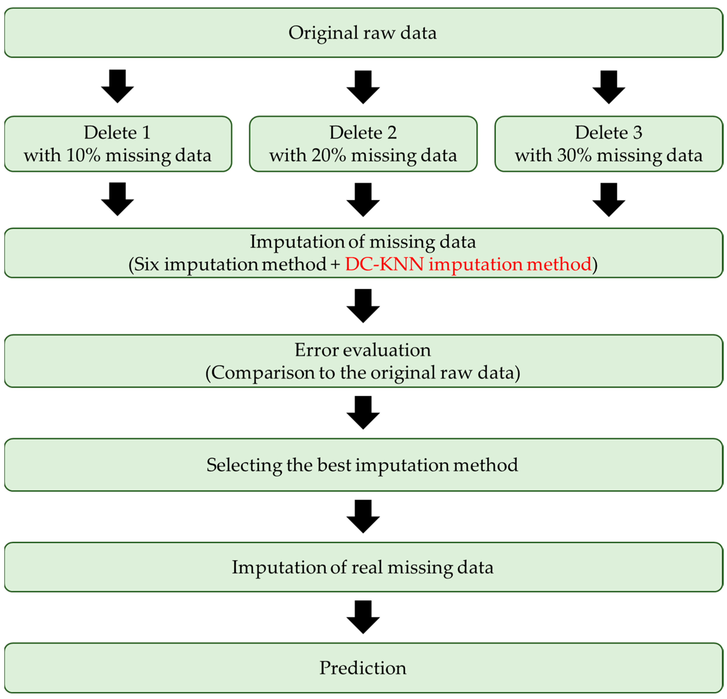
3. Research Methodology

3.1. Measurement Target and Period

This study was conducted on two 450 USRT-class turbo chillers installed on the third basement floor of Tower A in Seoul. Tower A is a 33-story commercial building with a total floor area of approximately 70,000 m², equipped with a central cooling system that operates under various conditions. Data were collected in real time through the building energy management system (BEMS) from March 2021 to July 2024. Due to the characteristics of cooling loads, measurements were taken only during the cooling season, from May to October.

During the daytime, the chiller operates under partial load while simultaneously utilizing the thermal energy storage (TES) system to handle the cooling load. At night, the system operates in a mode where ice is stored using capsule-type storage media. The cooling system in the study site operates under four primary modes:

A.

Ice-making mode: The process of freezing capsule-type media inside the thermal storage tank. The chiller is designed to operate at an average temperature of −4.5 °C. Ice storage primarily occurs during late-night hours, and the system stops after 10 h of operation or when the storage reaches 100% capacity;

B.

TES-only operation: The cooling load is handled solely by the thermal storage tank without operating the chiller. This mode is mainly used during transitional seasons or at night when the cooling demand is low;

C.

Parallel operation of the chiller and the TES: The chiller and the TES tank operate together to meet peak cooling loads. In this mode, the chiller operates at ambient conditions;

D.

Chiller-only operation: The chiller independently handles the cooling load without utilizing the TES system. This mode is used when the TES system malfunctions or when the thermal storage is completely depleted.

The collected data were processed by removing missing values and outliers from the original raw data. A partially missing-at-random (MAR) dataset with 10–30% missing values was then generated, and six imputation methods, including mean imputation, along with the DC-KNN imputation method, were applied to fill in the missing values. The imputed values were then compared with the actual values to identify the most effective imputation method. The final imputation accuracy was validated using the MAPE and CVRMSE, and the best-performing imputation method (DC-KNNs) was ultimately used to predict the actual missing values. Figure 2 illustrates the overall process [33].

3.2. Data Measurement

3.2.1. Data Measurement Method

For the performance analysis of the chillers, the study measured and recorded the flow rate and temperature of the chilled and cooling water, as well as the chiller’s power consumption. To measure the flow rate, an AUDS-100M ultrasonic flowmeter from AutoFLO (Bucheon-si, Gyeonggi-do, Republic of Korea) was used. This device is a time-difference ultrasonic flowmeter specifically designed for BEMS applications. The flowmeter uses a clamp-on sensor, allowing it to be attached externally without modifying the piping structure or cutting the pipe.

The temperature of the chilled and cooling water was measured using an NT-320G insertion-type temperature sensor from Hankyung Electric (Seoul, Republic of Korea). This sensor has a measurement range of −50 °C to 150 °C with an accuracy of ±0.5%, ensuring precise temperature data essential for chiller system performance analysis.

The chiller’s power consumption was measured using a GEMS3512 AC power meter from BMT (Yangsan-si, Republic of Korea). The collected data were transmitted via Modbus TCP communication to a direct digital controller (DDC), where they were later integrated and analyzed within the BEMS. Data for flow rate, temperature, and power consumption were transmitted in real time through RS485 communication and stored on the server at 15 min intervals. The types and key characteristics of the measurement equipment are summarized in

Table 1. Types and characteristics of measuring instruments.

Category	Ultrasonic Flow Meter	Temperature Sensor	AC Power Meter
Manufacturer	AutoFLO	Hankyung electric	BMT
Model	AUDS-100M	NT-320G	GEMS3512
Measurement principle	Transit time	Insertion type	CT or Rogowski coil
Measurement range	±0.02~15 m/s	−50~150 °C	0~415 VAC
Error	±1%	±0.5%	±0.5%

[33].

3.2.2. Uncertainty Analysis

To reliably evaluate the COP of the chiller, it is essential to consider the measurement uncertainty of the instruments used. In this study, the uncertainty of the measurement equipment listed in Table 1 was incorporated into the analysis. Generally, when a function R is determined by multiple measured variables $x_{1,}{x}_{2,}\cdots x_n$, the total uncertainty $W_R$ of the result R is calculated as follows [4]:

$$W_R=\sqrt{\sum {\left({\displaystyle \frac{\partial R}{{\partial x}_i}}{W}_{xi}\right)}^2}$$

(23)

During daytime operation, the COP was 4.04, and the total uncertainty $W_R$ at a 95% confidence level was determined to be ±0.073. In contrast, during nighttime operation, the COP was 2.26, with a corresponding $W_R$ ±0.036 at the same confidence level. These uncertainty values reflect the errors of the measurement instruments, and the analysis confirmed that the temperature sensors and power meters were the most significant contributors to COP uncertainty.

In addition to the uncertainties derived from instrument specifications, practical sources of error during data collection were also considered. The original power consumption data were measured using BEMS sensors with a rated accuracy of ±0.5%. To minimize the influence of abnormal values or sensor drift, EB filtering with a threshold of ±5% was applied.

Furthermore, the dataset was recorded at hourly intervals, which is appropriate for capturing the dynamic characteristics of chiller operation. The data spanned from May to October, encompassing a wide range of operational load conditions during the cooling season. By addressing these sources of uncertainty, the reliability of the imputation performance evaluation was further strengthened.

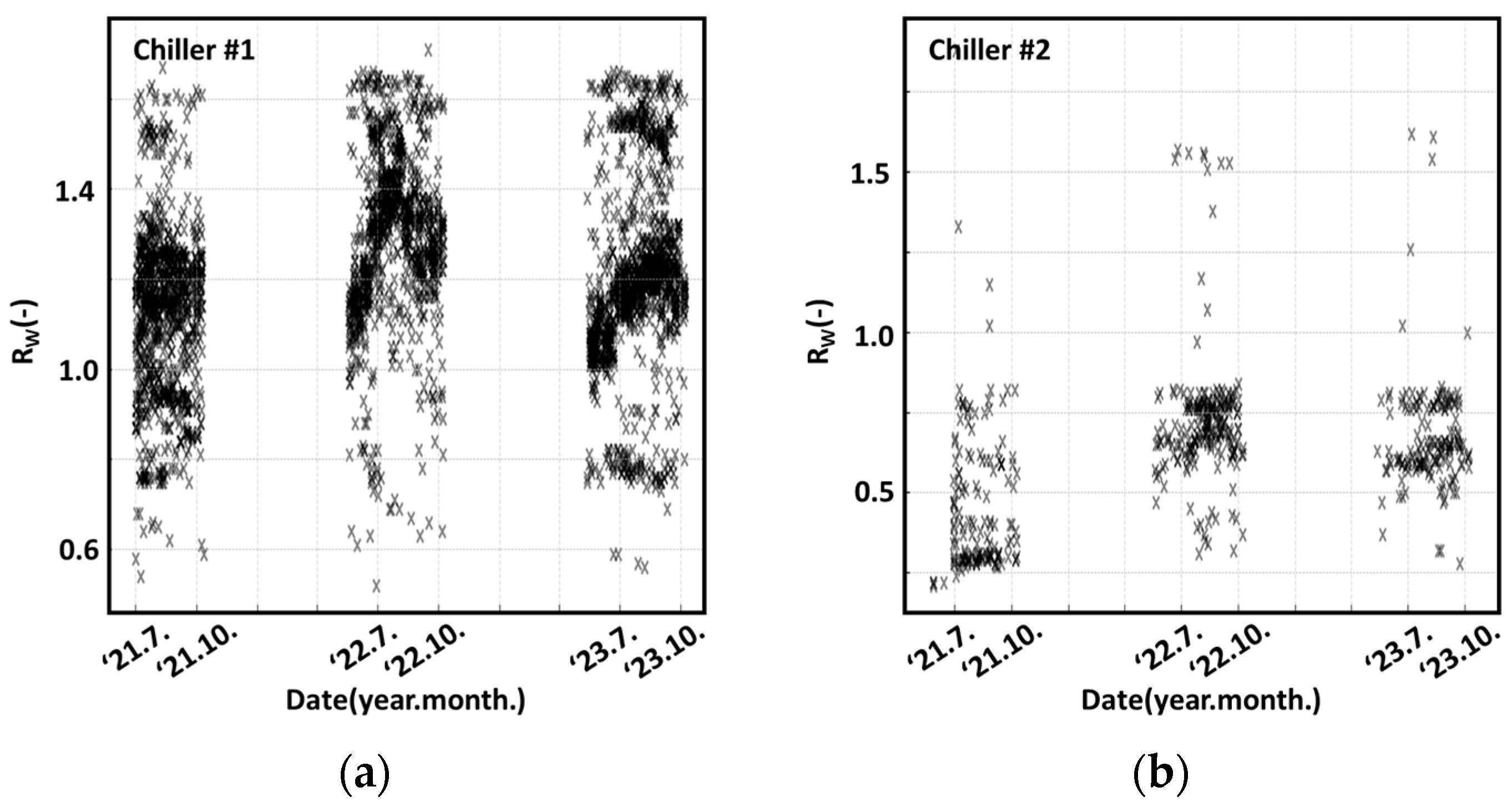
3.2.3. Initial Review of Collected Power Consumption Data

A total of 59,232 data points were collected from chiller #1 and another 59,232 from chiller #2, resulting in a total of 118,464 data points. At the study site, chillers operate using both direct cooling and the TES during the daytime (09:00–21:00), while at night (21:00–09:00), the chillers store ice. The collected data included chiller power consumption (${\dot{W}}_c$), which was analyzed based on the ratio of actual values to design values, as shown in

Table 2. Measured $R_W$ of chiller #1 and chiller #2.

Parameters	Chiller #1			Chiller #2
	59,232 Data Doints			59,232 Data Points
	Min	Mean	Max	Min	Mean	Max
$R_W$	0.01	0.94	42.10	0.01	0.89	51.70

. The formula for each series is as follows:

$$R_W={\displaystyle \frac{{\dot{W}}_o}{{\dot{W}}_a}}$$

(24)

$R_W$ is defined as the ratio of ${\dot{W}}_a$ to ${\dot{W}}_o$. This ratio serves as a critical indicator for evaluating how well the chiller operates relative to its designed capacity under the current operating conditions. The interpretation of the ratio is as follows [3]:

• $R_W>1$: The actual capacity exceeds the nominal capacity, indicating that the chiller is operating beyond its design conditions. This situation is typically caused by high load conditions or unexpected external environmental changes;
• $R_W=1$: The actual capacity matches the nominal capacity, meaning that the system is operating as per the design conditions;
• $R_W<1$: The actual capacity is lower than the nominal capacity, suggesting that the chiller is operating under partial load conditions. This state frequently occurs in energy-saving modes or low-load conditions.

From the 118,464 collected data points (chiller #1: 59,232, chiller #2: 59,232), the missing values and outliers were identified and separated (

Table 3. The missing data for ${\dot{W}}_c$ in chiller #1 and chiller #2.

Parameters	Chiller #1		Chiller #2
	59,232 Data Points		59,232 Data Points
	Daytime	Nighttime	Daytime	Nighttime
Missing data	26,838	16,460	24,727	14,789
$\mathrm{O}\mathrm{u}\mathrm{t}\mathrm{l}\mathrm{i}\mathrm{e}\mathrm{r}$ data	1474	8769	3504	12,493

). Outliers were defined as data points falling outside the ±5% energy balance error (EB) range [11,12].

To analyze the distribution of ${\dot{W}}_c$, the hourly variation of $R_W$ was examined using the raw dataset. As shown in Figure 3, valid data points appeared only between May and October, reflecting the seasonal operation of the chiller system. This figure serves as a baseline reference to define the effective data period for subsequent preprocessing and experimental scenario construction.

3.2.4. Review of Valid Data

The valid data preprocessed based on the EB (±5%) consists of 3236 entries for chiller #1 and 524 entries for chiller #2 (

Table 4. Appropriate $R_W$ for chiller #1–#2.

Parameters	Chiller #1			Chiller #2
	3236 Data Points			524 Data Points
	Min	Mean	Max	Min	Mean	Max
$R_W$	0.52	1.21	1.71	0.21	0.64	1.88

).

The time-based variation of $R_W$ was re-examined after applying missing value and outlier removal, as shown in Figure 4. Compared to the raw data in Figure 3, a substantial reduction in data points is observed, reflecting the impact of preprocessing. This figure serves to verify the effectiveness of the EB (±5%) filtering process and define the cleaned dataset used as the baseline for subsequent imputation experiments.

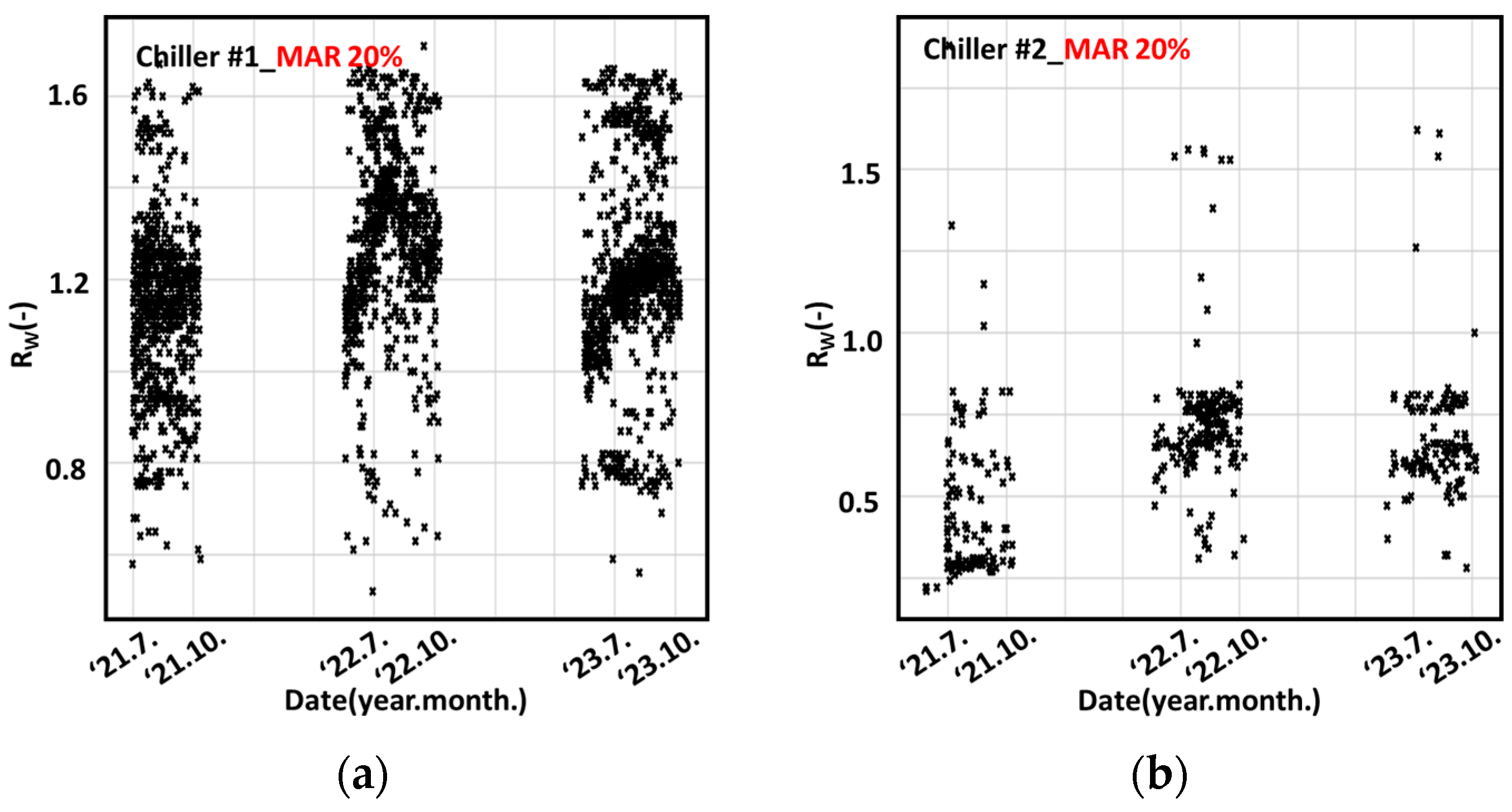
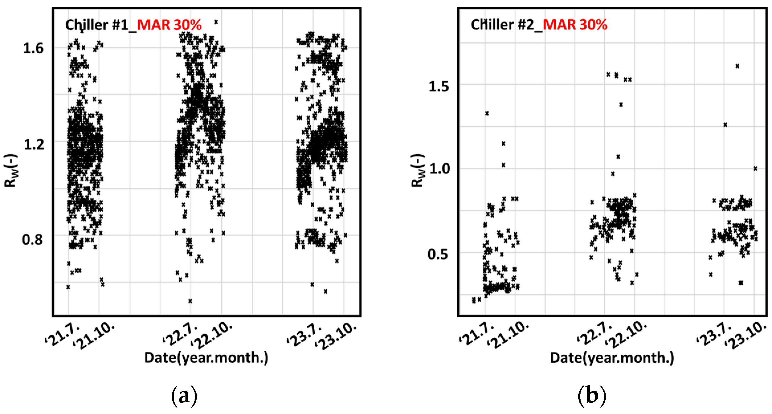
3.3. Partially MAR Data

A total of 3236 values of $R_W$ from chiller #1 and 524 from chiller #2 were artificially removed using the missing-at-random (MAR) assumption, based on the preprocessed dataset filtered by the EB (±5%). To evaluate the robustness of the imputation algorithms under increasing levels of data loss, the missingness was categorized into 10% (Figure 5), 20% (Figure 6), and 30% (Figure 7) scenarios. These figures visualize the spatial and temporal distribution of the missing values introduced at each level, serving as references for the experimental conditions defined in

Table 5. The number of missing data under MAR 10–30% conditions for chillers #1–#2.

Parameters	Chiller #1		Chiller #2
	3236 Data Points		524 Data Points
	Remain	Missing	Remain	Missing
MAR 10%	2913	323	472	52
MAR 20%	2589	647	420	104
MAR 30%	2266	970	367	157

.

To implement the MAR condition, missing values were applied to the power consumption variable ${\dot{W}}_c$ with conditional dependence on the observed variables $T_1$, $T_2$, $T_3$, $T_4$, ${\dot{V}}_1$ and ${\dot{V}}_3$. This ensures that the probability of a missing value occurring in ${\dot{W}}_c$ depends on other observed values in accordance with the MAR framework. The missing data were introduced in stages: an initial 10% of records were randomly selected based on these conditions, followed by an additional 10% (cumulative 20%) and a final 10% (cumulative 30%), each applied to the remaining observed data. This incremental approach preserved the MAR logic while controlling the overall missingness.

According to the MAR framework, missing values are assumed to be dependent on other observed variables but not on the missing values themselves, allowing for statistically valid imputations based on the available data [31]. The corresponding mathematical expression is presented below:

$$P\left(R|Y_{obs},Y_{mis}\right)=P\left(R\right|Y_{obs})$$

(25)

4. Experimental Results and Discussion

4.1. Results of Replacing Partially Missing-at-Random Data

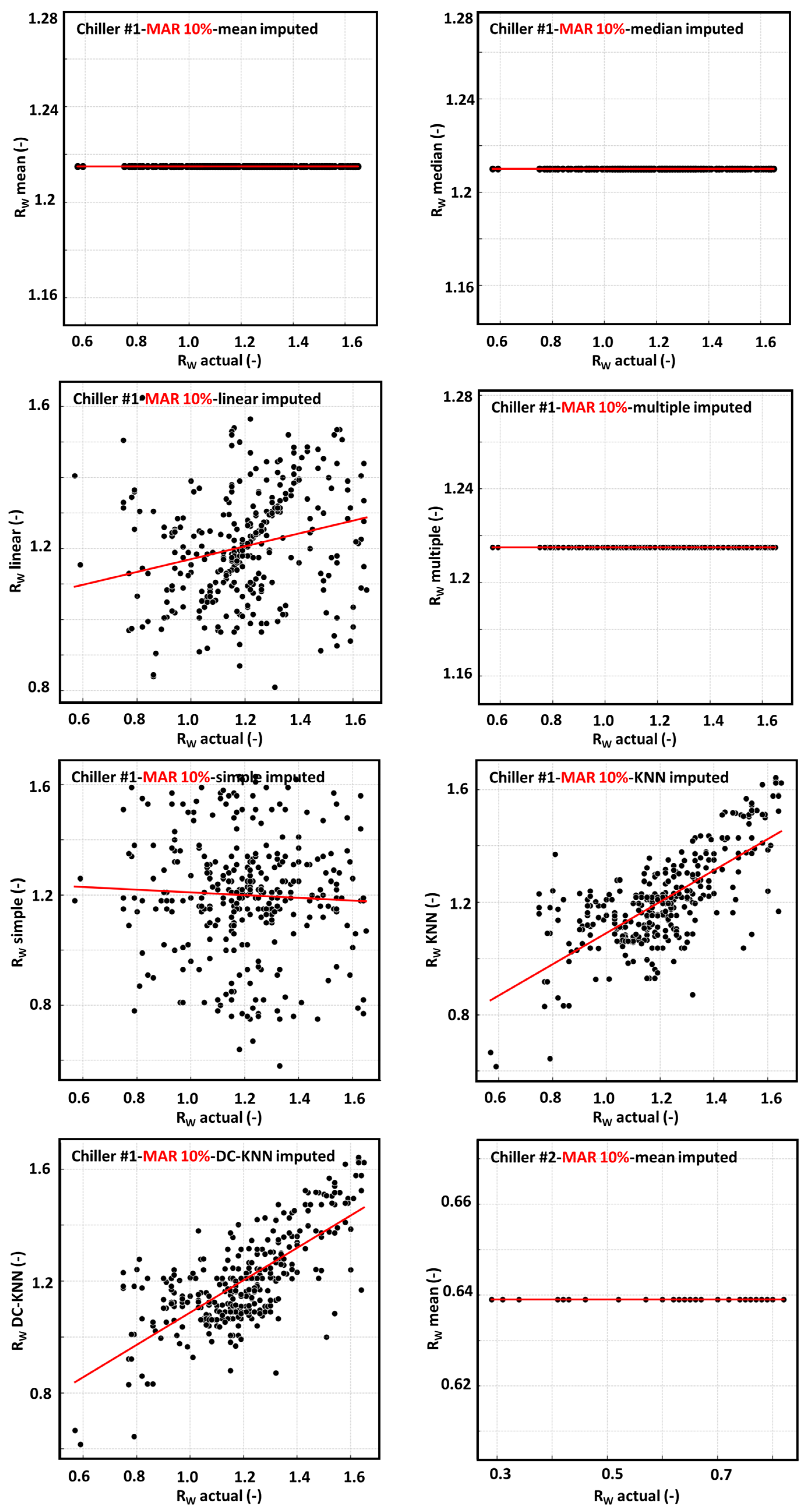
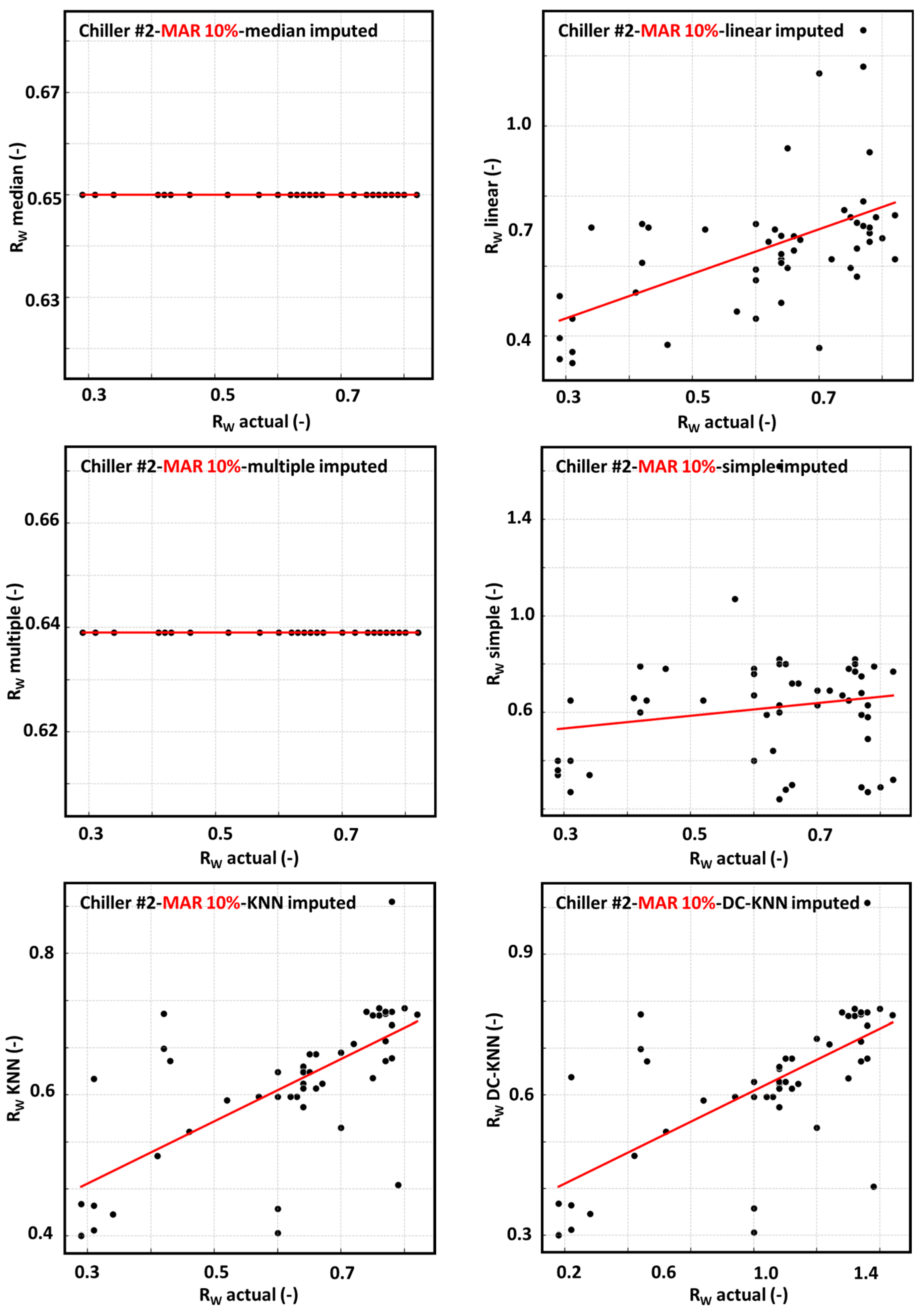
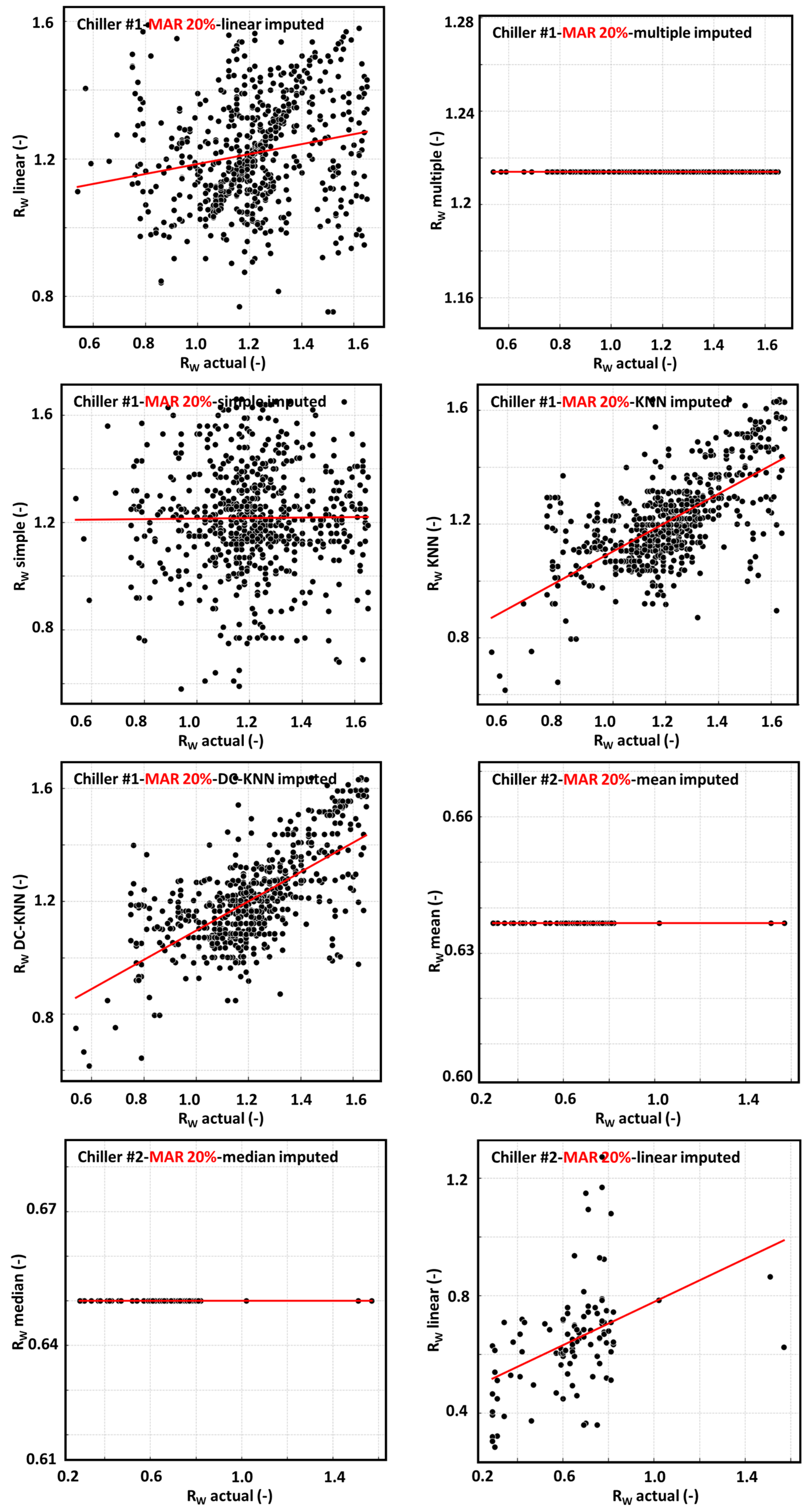
4.1.1. Mean Imputation

In terms of the MAPE, chiller #1 showed a stable performance across the MAR levels, with values of 14.62% at 10%, 14.28% at 20%, and 14.69% at 30%. Chiller #2 followed a similar trend with 13.76%, 13.52%, and 13.86%, respectively. The error rates remained relatively consistent, indicating that mean imputation is resilient to increasing missingness in terms of average accuracy.

For the CVRMSE, chiller #1 recorded 17.43%, 17.33%, and 17.65%, while chiller #2 showed slightly lower variability at 16.91%, 16.66%, and 17.01% across the same MAR levels. This suggests that the mean imputation maintains moderate predictive stability and is particularly effective when the goal is to minimize model complexity and preserve central tendencies (

Table 6. Results of MAR imputation validation.

Method	MAR	Chiller #1		Chiller #2
		MAPE	CVRMSE	MAPE	CVRMSE
Mean	10%	14.62%	17.43%	13.76%	16.91%
	20%	14.28%	17.33%	13.52%	16.66%
	30%	14.69%	17.65%	13.86%	17.01%
Median	10%	14.96%	17.66%	14.06%	17.13%
	20%	14.71%	17.63%	13.87%	16.94%
	30%	15.10%	17.94%	14.22%	17.27%
Linear	10%	14.57%	19.39%	14.44%	18.98%
	20%	15.08%	19.81%	14.26%	18.79%
	30%	15.37%	20.06%	14.61%	19.08%
Multiple	10%	14.62%	17.43%	13.76%	16.91%
	20%	14.28%	17.33%	13.52%	16.66%
	30%	14.69%	17.65%	13.86%	17.01%
Simple	10%	21.51%	25.78%	20.94%	24.98%
	20%	20.27%	23.95%	20.14%	23.81%
	30%	21.15%	25.02%	20.53%	24.46%
KNNs	10%	9.92%	12.37%	10.04%	12.87%
	20%	10.23%	13.20%	10.42%	13.41%
	30%	10.35%	13.23%	10.58%	13.62%
DC-KNNs	10%	9.86%	12.19%	9.74%	12.65%
	20%	10.30%	13.19%	10.17%	13.32%
	30%	10.08%	13.06%	10.29%	13.43%

).

Mean imputation replaces all missing entries with a single average value, resulting in a horizontally aligned distribution. While this approach is computationally efficient and robust against outliers, it reduces natural variance in the data and can mask underlying patterns. Thus, it is best suited for datasets with low missingness and when preserving structural variation is not critical (Figure 8, Figure 9 and Figure 10).

4.1.2. Median Imputation

For the MAPE, chiller #1 recorded 14.96%, 14.71%, and 15.10% at MAR levels of 10%, 20%, and 30%, respectively, indicating a slight degradation in accuracy as the missing rate increased. Chiller #2 displayed comparable results with 14.06%, 13.87%, and 14.22%, suggesting stable and consistent imputation performance across varying levels of missingness.

In terms of the CVRMSE, chiller #1 maintained values of 17.66%, 17.63%, and 17.94%, while chiller #2 showed slightly lower variation with 17.13%, 16.94%, and 17.27%, respectively. These results confirm that median imputation offers reliable performance in terms of both accuracy and variance, especially in datasets with modest outlier presence (Table 6).

Similar to mean imputation, median imputation substitutes missing values with a single central tendency value. However, unlike the mean, the median is robust to extreme outliers, making it preferable in skewed distributions or datasets with anomalies. Although it preserves the central location of the data more effectively than the mean, it still reduces variability and fails to capture the dynamics of temporal or correlated variables. Therefore, it is most appropriate for non-time-series data with a relatively low to moderate rate of missingness and the presence of outliers (Figure 8, Figure 9 and Figure 10).

4.1.3. Linear Interpolation

For the MAPE, chiller #1 showed a slight increase across missingness levels, with 14.57%, 15.08%, and 15.37% at MAR 10%, 20%, and 30%, respectively. Chiller #2 followed a similar trend with values of 14.44%, 14.26%, and 14.61%. These results suggest that while linear interpolation maintains moderate accuracy at lower missing rates, its performance degrades slightly as the extent of missingness increases.

Regarding the CVRMSE, chiller #1 exhibited relatively higher variability compared to other methods, with 19.39%, 19.81%, and 20.06% at MAR 10%, 20%, and 30%. Chiller #2 also recorded increasing variability, with 18.98%, 18.79%, and 19.08%, indicating that linear interpolation is more susceptible to data pattern distortion, particularly in highly dynamic time-series environments (Table 6).

Linear interpolation estimates missing values by connecting known values on either side with a straight line, thereby assuming smooth transitions between points. This results in a diagonally aligned imputation structure, which is effective in preserving local continuity and trends in sequential datasets. However, it lacks the flexibility to capture nonlinear fluctuations or abrupt shifts, especially when large consecutive gaps exist. Thus, while linear interpolation is suitable for temporally continuous data with mild variability, its performance may be limited in systems with sharp transitions or complex dynamics (Figure 8, Figure 9 and Figure 10).

4.1.4. Multiple Imputation

For the MAPE, chiller #1 showed consistent accuracy across missingness levels, recording 14.62%, 14.28%, and 14.69% at MAR 10%, 20%, and 30%, respectively. Chiller #2 exhibited very similar results with 13.76%, 13.52%, and 13.86%, indicating that multiple imputation maintains stable predictive accuracy regardless of the proportion of missing data. This trend suggests that multiple imputation is robust to increased missingness, particularly when the data distribution remains relatively consistent.

In terms of the CVRMSE, chiller #1 maintained steady variability with values of 17.43%, 17.33%, and 17.65%, showing minimal deviation across the MAR levels. Chiller #2 also demonstrated low and stable variability, with 16.91%, 16.66%, and 17.01%. These results indicate that multiple imputation effectively preserves the variance structure of the original dataset across both chillers (Table 6).

Unlike single-value replacement methods such as mean or median imputation, multiple imputation involves generating multiple plausible values based on probabilistic modeling. These imputed values are then aggregated to form a more realistic estimate that reflects the underlying distribution. This approach helps to retain natural variability and improves inference quality.

The strengths of multiple imputation include enhanced statistical validity, the ability to handle uncertainty, and improved performance in downstream analysis. However, it requires more computational resources and methodological rigor and is sensitive to the assumptions underlying the imputation model. Overall, it is well-suited for cases where maintaining distributional integrity and prediction robustness is critical, especially in the context of machine learning model preparation or inferential studies (Figure 8, Figure 9 and Figure 10).

4.1.5. Simple Random Imputation

For the MAPE, chiller #1 recorded 21.51%, 20.27%, and 21.15% at MAR levels of 10%, 20%, and 30%, respectively, indicating high and inconsistent error rates across different missingness levels. Similarly, chiller #2 exhibited substantial errors with MAPE values of 20.94%, 20.14%, and 20.53%. These results demonstrate that simple random imputation offers low accuracy and limited robustness, particularly in structured, time-dependent datasets, such as chiller sensor records.

In terms of the CVRMSE, chiller #1 recorded 25.78%, 23.95%, and 25.02%, while chiller #2 showed 24.98%, 23.81%, and 24.46% at MAR 10%, 20%, and 30%, respectively. These values are the highest among all tested methods, highlighting the poor ability of simple random imputation to preserve data variability and predictive fidelity (Table 6).

Simple random imputation involves replacing missing values with randomly sampled values from the observed dataset without considering time order, contextual similarity, or feature relationships. While this method may minimize systematic bias, it introduces high variance and disrupts temporal or structural dependencies within the data. This often leads to noisy imputations and degraded model performance in both analytical and predictive tasks.

Due to its disregard for pattern integrity and sequence continuity, simple random imputation is generally unsuitable for time-series or sensor data. Its application is discouraged except in exploratory contexts or for benchmarking purposes where simplicity is prioritized over accuracy (Figure 8, Figure 9 and Figure 10).

4.1.6. KNN Imputation

For the MAPE, chiller #1 showed 9.92%, 10.23%, and 10.35% at MAR levels of 10%, 20%, and 30%, respectively, while chiller #2 recorded 10.04%, 10.42%, and 10.58% for the same missingness levels. These results indicate that KNN imputation maintains relatively consistent and moderate error rates, even as the proportion of missing data increases, suggesting robustness across varying levels of data incompleteness.

In terms of the CVRMSE, chiller #1 yielded 12.37%, 13.20%, and 13.23%, and chiller #2 exhibited 12.87%, 13.41%, and 13.62% across the respective MAR levels. While not the lowest among the tested methods, these values indicate stable variability control, particularly when compared to more simplistic imputation techniques (Table 6).

KNN imputation identifies the K most similar complete records (neighbors) based on a defined distance metric—commonly the Euclidean distance—and imputes missing values using a weighted or unweighted aggregation of those neighbors. This method preserves local data structure, capturing both linear and nonlinear relationships, making it particularly effective in datasets with complex inter-feature interactions.

However, its performance is sensitive to the choice of hyperparameters such as K and the distance metric. Additionally, KNNs can suffer from high computational cost and diminished accuracy when dealing with sparse datasets or high proportions of missingness. Despite these limitations, the KNN method offers a balanced trade-off between performance and flexibility, making it a strong candidate for structured sensor datasets where local contextual information is important (Figure 8, Figure 9 and Figure 10).

4.1.7. DC-KNN Imputation

For the MAPE, chiller #1 recorded 9.86%, 10.30%, and 10.08% at MAR levels of 10%, 20%, and 30%, respectively, while chiller #2 showed 9.74%, 10.17%, and 10.29%. These results indicate that DC-KNN imputation maintains stable and competitive accuracy, with slightly improved performance over standard KNNs, particularly at lower MAR levels.

In terms of the CVRMSE, chiller #1 yielded 12.19%, 13.19%, and 13.06%, while chiller #2 showed 12.65%, 13.32%, and 13.43%. The consistent and controlled variability across missingness rates suggests that DC-KNN imputation is robust in preserving underlying data characteristics, even under increased data sparsity (Table 6).

DC-KNN imputation improves upon conventional KNNs by integrating dynamic weighting of variables and cluster-based neighbor selection. Rather than selecting neighbors solely based on global distance, the DC-KNN method first identifies clusters of data with similar patterns—such as those defined by temperature or flow rate levels—and restricts neighbor search within the same cluster. This structure-sensitive approach increases the contextual relevance of the selected neighbors.

Furthermore, the DC-KNN method introduces variable-specific weighting that balances between Euclidean distance and cosine similarity depending on feature characteristics, allowing more flexible modeling of both magnitude and directional relationships. This enhances the fidelity of the imputed values while mitigating distortion caused by irrelevant neighbors.

While the method incurs higher computational cost and complexity, its advantages lie in its ability to maintain structural consistency and increase imputation realism, particularly in multidimensional and time-series sensor datasets. It is especially suitable for preprocessing stages in high-stakes predictive modeling, where data integrity and precision are essential (Figure 8, Figure 9 and Figure 10).

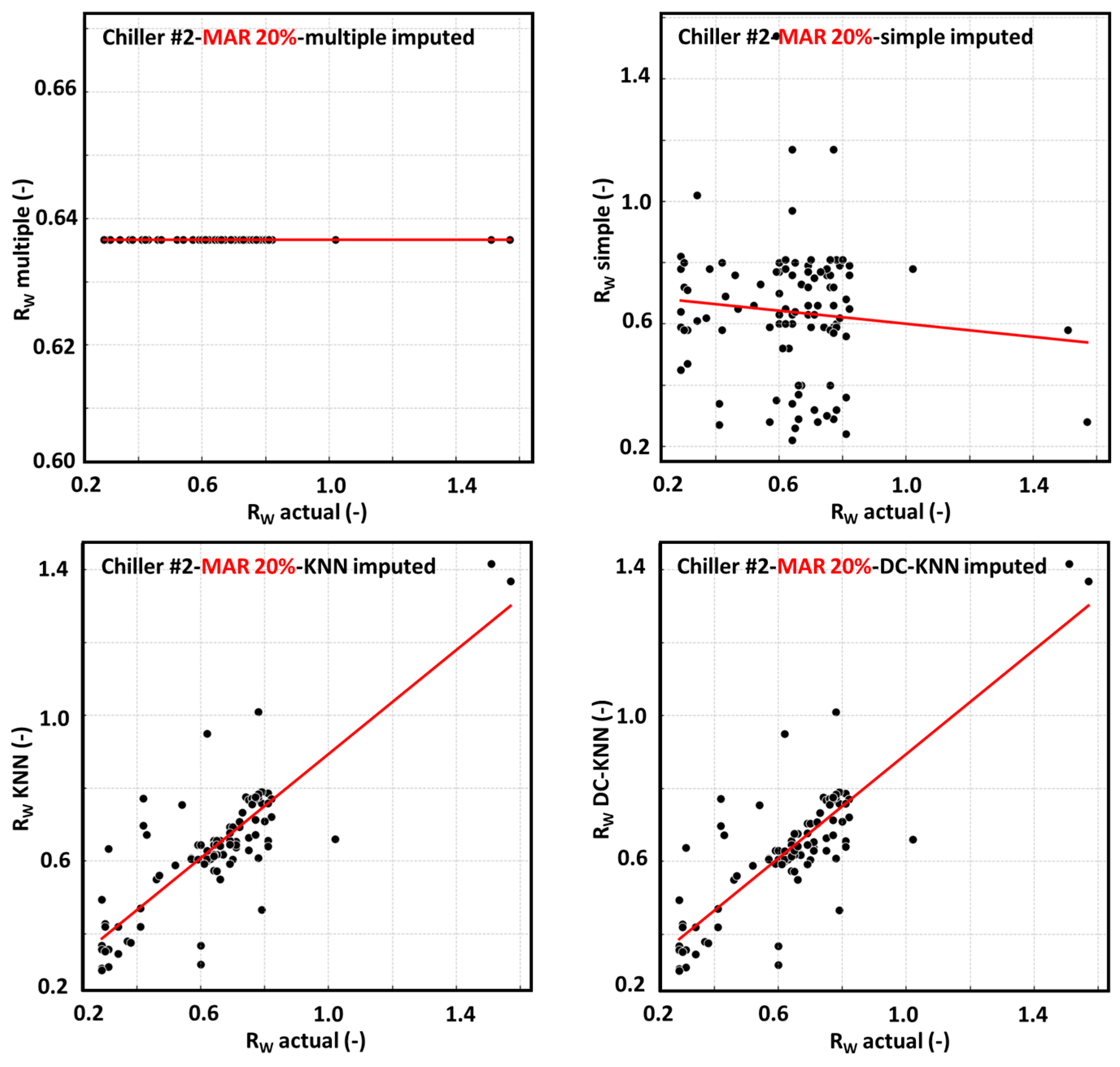
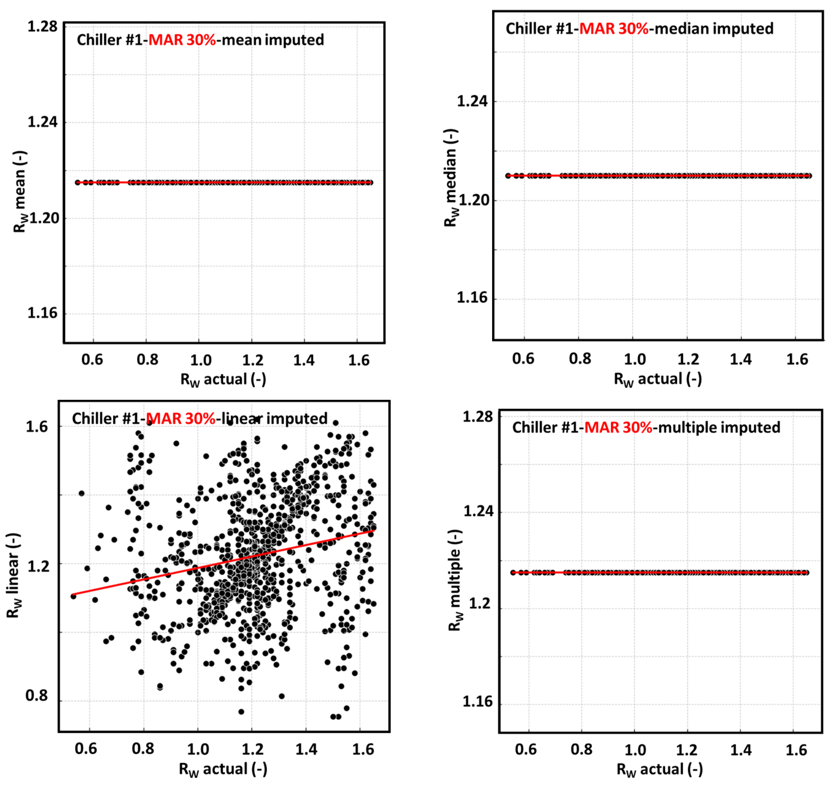
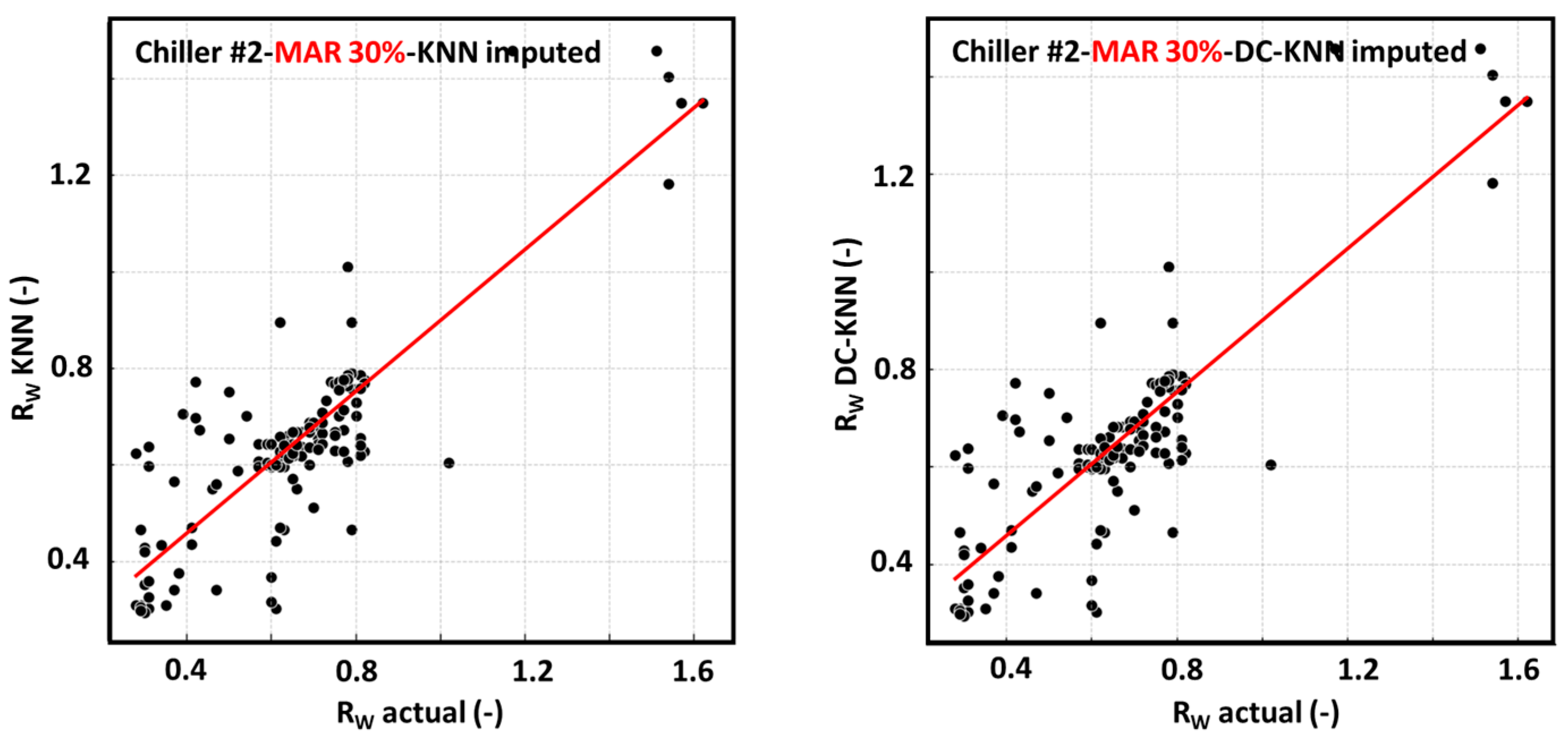
4.1.8. Visual Comparison and Interpretation of Algorithm Performance

Figure 8, Figure 9 and Figure 10 present a comparative visualization of the prediction performance of seven imputation methods under three MAR conditions (10%, 20%, and 30%) using MAPE as the evaluation metric. Each figure illustrates how the accuracy of each method varies across chiller #1 and #2, providing a clear depiction of how performance differences evolve as the level of missingness increases.

The proposed DC-KNN method consistently achieved the lowest or near-lowest MAPE values across all missingness levels, demonstrating strong accuracy and robustness. In particular, it outperformed conventional KNNs under higher missing rates, indicating that its cluster-based neighbor selection and dynamic weighting mechanisms effectively capture the underlying structure of the data.

By separating the figures by missingness level, the layout enables an assessment not only of absolute performance but also of the stability and scalability of each method under increasing data sparsity. This visual evidence supports the conclusion that the DC-KNN method is not only precise but also structurally superior in preserving contextual integrity in time-series sensor environments.

4.2. Selection of Optimal Imputation Methods

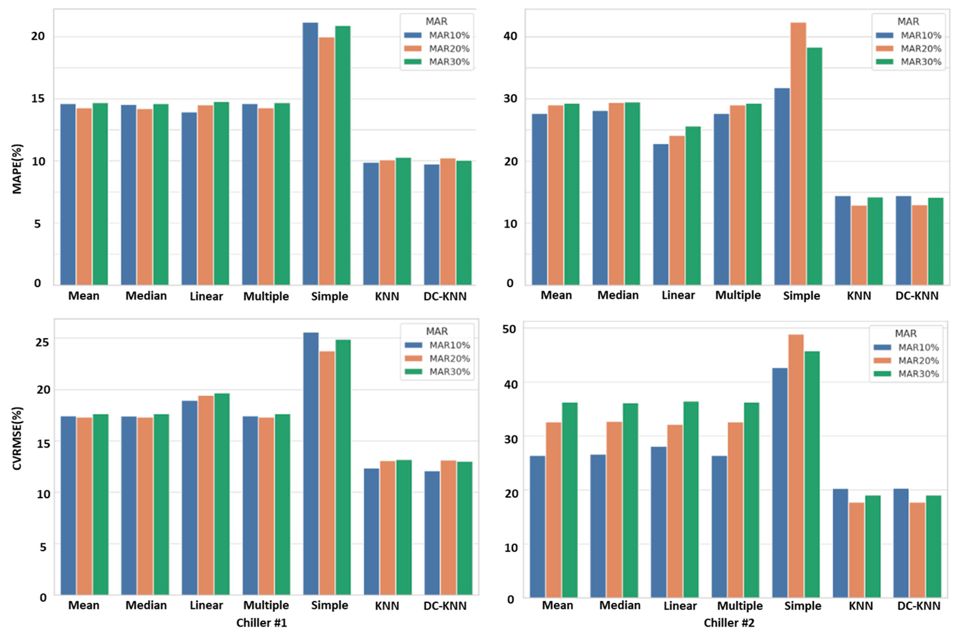
4.2.1. Optimal Imputation Method Based on MAPE

DC-KNNs consistently achieved the lowest MAPE across all MAR levels for both chiller #1 and chiller #2, demonstrating the highest level of accuracy among all evaluated methods. Specifically, DC-KNNs recorded 9.86%, 10.30%, and 10.08% for chiller #1, and 9.74%, 10.17%, and 10.29% for chiller #2 at MAR 10%, 20%, and 30%, respectively. These results reflect DC-KNNs’ superior ability to minimize absolute predictive error. Although KNNs also maintained competitive performance, it was consistently outperformed by DC-KNNs, particularly at lower MAR levels. In contrast, simple random imputation recorded the highest MAPE across all conditions, indicating poor performance and high volatility. These findings affirm that DC-KNNs provide the most accurate imputation across various degrees of data sparsity (Figure 11).

4.2.2. Optimal Imputation Method Based on CVRMSE

For the CVRMSE, the DC-KNN method again demonstrated strong performance, especially for chiller #2, where it recorded the lowest variability at all MAR levels (12.65%, 13.32%, 13.43%). For chiller #1, while mean, median, and multiple imputation performed slightly better at MAR 10%, DC-KNNs remained highly competitive and recorded lower error rates than KNNs and all other methods as the MAR increased. By contrast, simple random imputation produced the highest CVRMSE values for both chillers, highlighting its limited reliability for variance-sensitive applications. These results emphasize the robustness of DC-KNNs in preserving not only accuracy but also the variance structure of the data (Figure 11).

4.2.3. Changes According to MAR Levels

All imputation methods exhibited increasing MAPE and CVRMSE values as the MAR level rose, reflecting the inherent challenge of accurately recovering missing information under high data sparsity. Notably, simple random imputation, linear interpolation, and KNNs showed steep performance degradation at MAR 30%, demonstrating sensitivity to missing data proportions. In contrast, DC-KNNs and multiple imputation maintained stable performance across all MAR levels. Their resilience under high missingness suggests suitability for robust imputation in real-world applications where complete data availability cannot be guaranteed (Figure 11).

4.2.4. Derivation of the Optimal Imputation Method

Considering both error metrics—the MAPE and the CVRMSE—the DC-KNN imputation was identified as the most reliable and versatile method. Its hybrid architecture, which integrates clustering, dynamic weighting, and distance-based neighbor selection, allows it to adapt effectively to the structural characteristics of chiller sensor data. While mean, median, and multiple imputation methods provided reasonable performance at lower MAR levels and may be suitable for simple scenarios, their limitations become more apparent as the missing rate increases. Linear interpolation, although preserving continuity, struggled under high missingness, and simple random imputation proved inadequate across all conditions. Therefore, the DC-KNN approach is recommended as the optimal imputation method for both accuracy and robustness in high-dimensional, time-dependent sensor datasets (Figure 11).

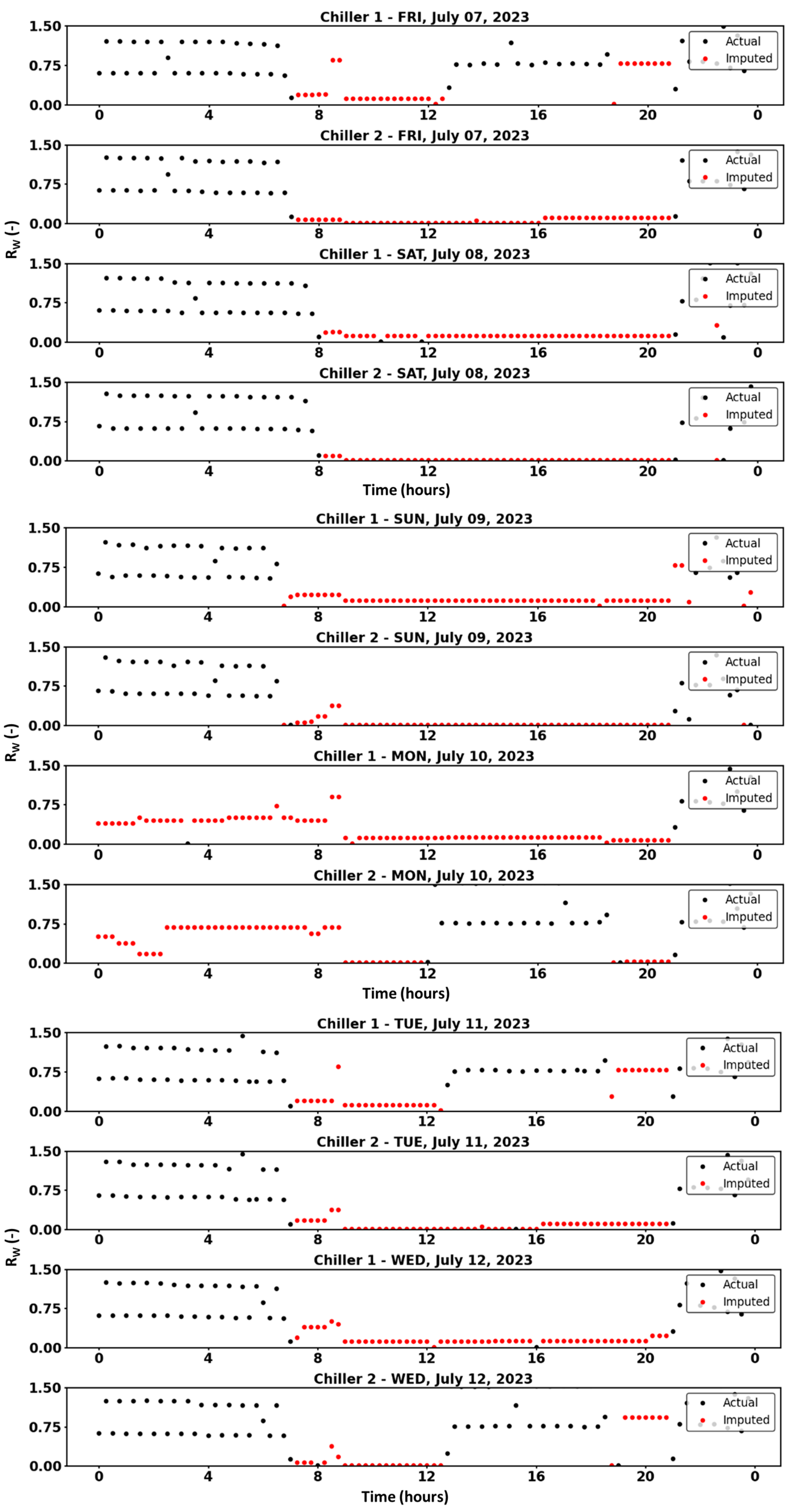
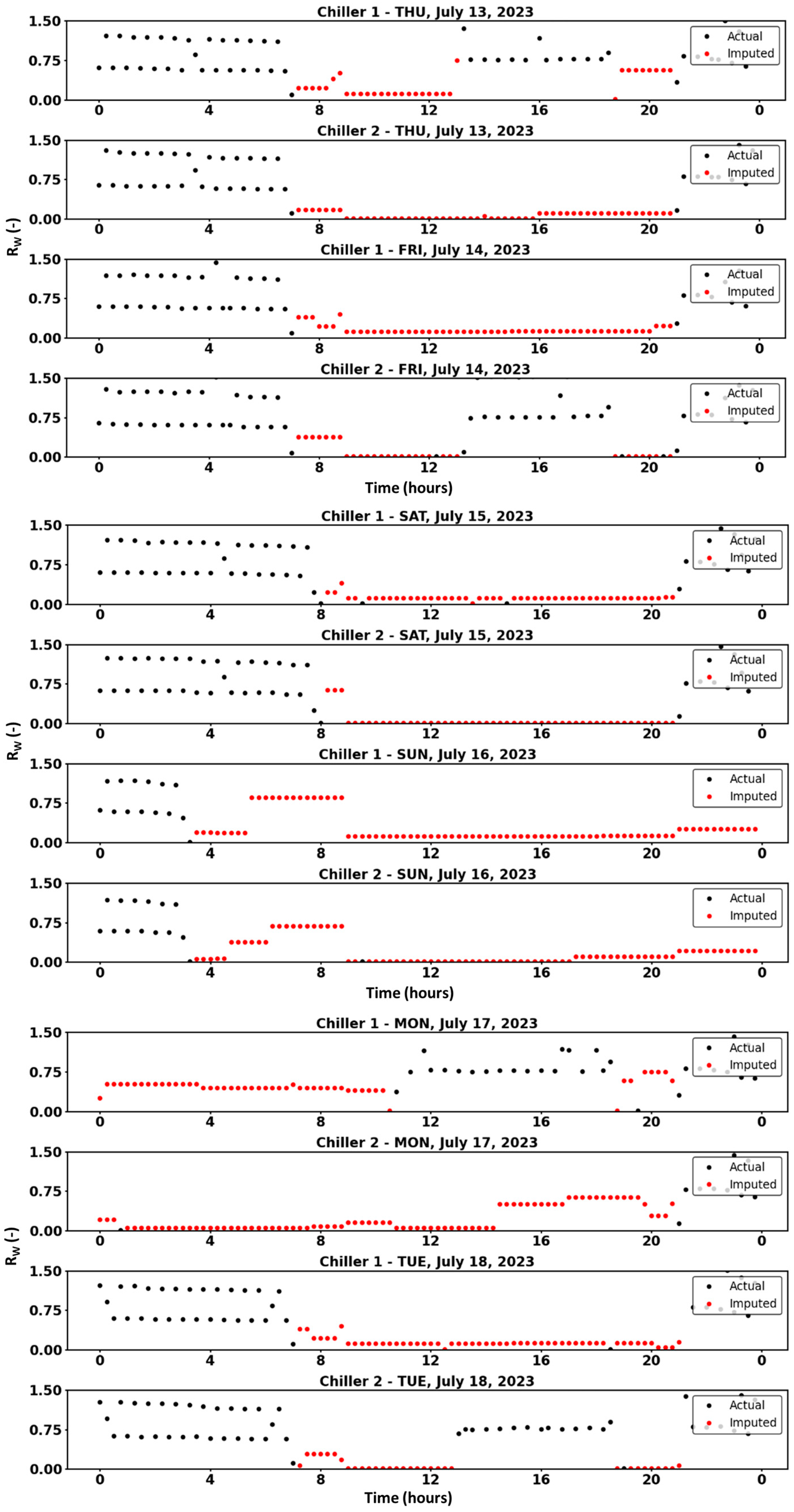
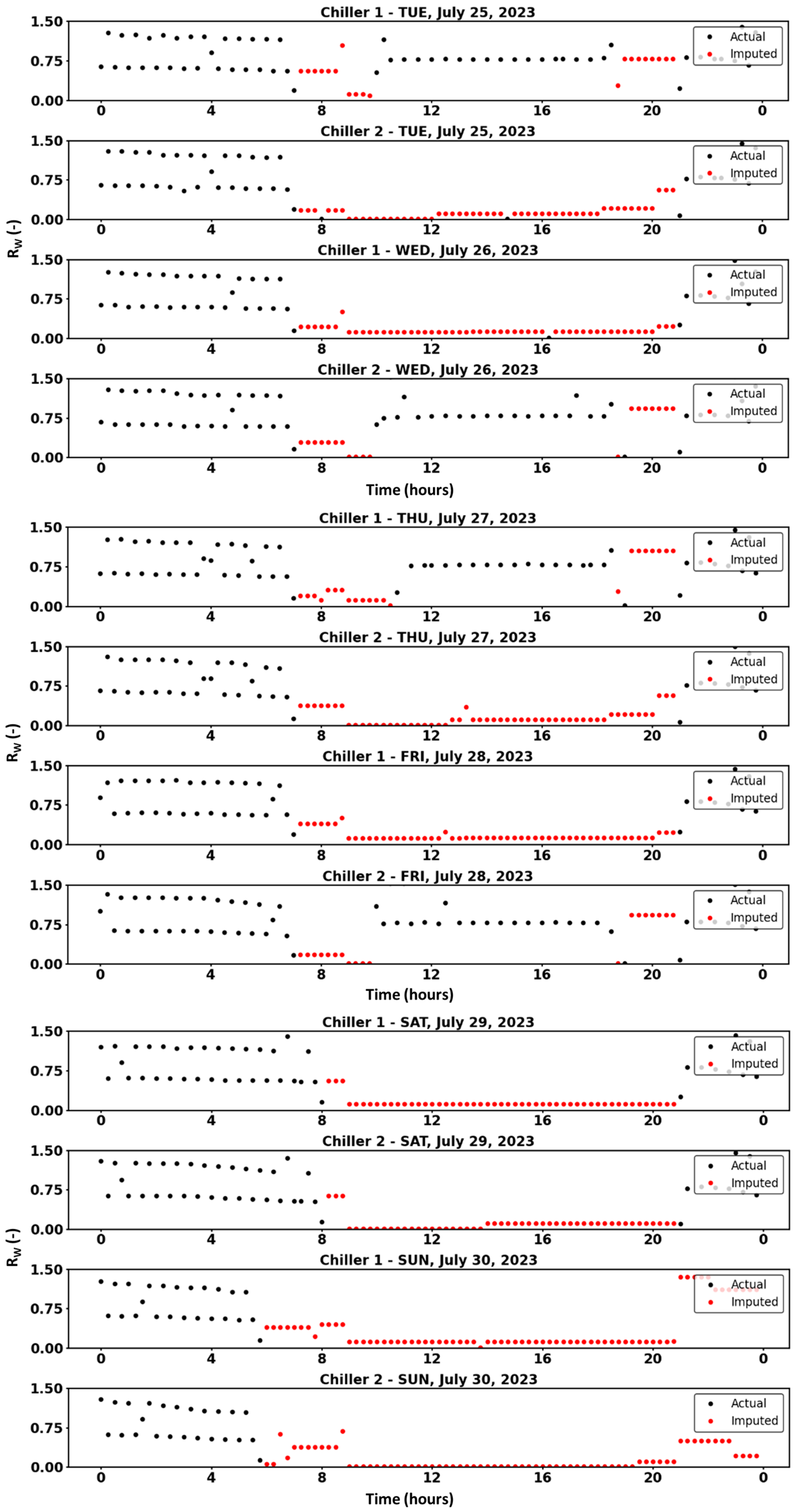
4.3. DC-KNN Imputation for Actual Missing Data

Using raw data spanning a total of three years, the missing values of $R_W$ for chiller #1 and chiller #2 in July 2023 were imputed using the DC-KNN method. Given the site characteristics, the power consumption of the chiller can be significantly low when utilizing thermal energy storage, and the imputed values appear to reflect this characteristic. The black points represent actual values, while the red points indicate imputed values (Figure 12).

5. Discussion

Various missing data imputation techniques were compared and analyzed for the power consumption records of water-cooled centrifugal chillers, and the performance of the proposed DC-KNN method was evaluated accordingly. The DC-KNN method was designed to overcome the limitations of conventional KNN-based imputation by integrating K-means clustering to guide neighbor selection within localized operational contexts and applying dynamic weights based on feature-specific characteristics. This approach enables a more precise reflection of the physical behavior of the data.

The use of Euclidean distance for similarity measurement, cluster-based neighbor selection, and inverse-distance weighted averaging proved effective in preserving the structural consistency of the chiller operation data. When applied under missing-at-random (MAR) conditions with missing rates ranging from 10% to 30%, the DC-KNN method consistently outperformed conventional approaches—including mean, median, linear interpolation, multiple imputation, simple random imputation, and standard KNNs—in terms of both MAPE and CVRMSE.

Specifically, the DC-KNN method maintained a stable performance with MAPE values below 10% across all missingness levels for both chiller #1 and chiller #2 and demonstrated lower variability in the CVRMSE compared to other methods. These results suggest that the DC-KNN approach effectively restores underlying patterns and variance structures, even under high missingness conditions. In contrast, methods such as simple random imputation and linear interpolation showed significant performance degradation as the missing rate increased, whereas the DC-KNN method maintained robustness, indicating its high practical applicability.

However, the performance gap among imputation methods was not statistically large in all cases; particularly under low missingness, multiple imputation and even mean substitution also exhibited a relatively strong performance. Thus, in practical settings, a flexible choice among various validated imputation methods—including DC-KNNs—can be made based on data characteristics and the nature of missingness. Applying advanced methods, such as DC-KNNs, may further enhance data quality where complex or structured missing patterns are present.

It is also noted that the DC-KNN method may be sensitive to certain hyperparameters, such as the number of clusters (K) and distance-based weighting schemes, and its computational cost may increase with large-scale datasets. Future work should explore automated cluster optimization and algorithmic improvements to enhance scalability and efficiency.

On the other hand, although the DC-KNN method demonstrated superior performance in terms of imputation accuracy due to its cluster-based local interpolation mechanism, the algorithm inherently requires repeated execution of K-means clustering and KNN searches within each cluster. This structure can lead to increased computational time, particularly in large-scale datasets or real-time streaming environments.

While this study was conducted using a static dataset and did not include measurements of real-time computational load, future research should consider lightweight adaptations—such as online clustering, approximate KNNs, or parallel processing-based implementations—to improve computational efficiency.

In practical applications such as building energy management systems (BEMSs) or digital twin platforms, real-time processing capability is as critical as accuracy. Therefore, adapting the structure of the DC-KNN method to meet the requirements of real-time control environments will be an essential direction for its practical advancement.

While deep learning-based imputation methods, such as BiLSTM and autoencoders, have recently gained attention in time-series recovery tasks, this study focused on interpretable and practically applicable methods based on statistical and tree-based models. Deep learning-based approaches are currently under investigation in a separate follow-up study, with a focus on sequence learning, nonlinear dynamic pattern recognition, and model generalizability for energy forecasting and real-time control in chiller systems.

Beyond technical improvements in imputation accuracy, the reliability of restored sensor data plays a critical role in enabling data-driven decision-making in intelligent energy systems. Similarly, Es-sakali et al. [34] developed a predictive maintenance strategy based on real-time monitoring of a VRF system installed in an actual building, highlighting the importance of comprehensive data preprocessing—including missing value imputation, outlier removal, and noise filtering—for accurate fault diagnosis and energy efficiency optimization.

Their comparative analysis of multiple machine learning models demonstrated that data quality is a decisive factor in the effectiveness of predictive maintenance. These findings support the practical applicability and technical value of the proposed DC-KNN method, especially in scenarios where restored data serve as the foundation for high-stakes decision-making in intelligent HVAC control systems [34].

Prior studies in soft science fields have emphasized the importance of trustworthy data in supporting predictive maintenance, operational optimization, and adaptive energy control strategies in smart building environments [35]. The DC-KNN method proposed in this study preserves interpretability while enhancing accuracy under high-missingness conditions, making it a promising candidate for integration into real-time control architectures and context-aware decision frameworks.

In sensor-based energy management systems, the reliability and completeness of input data are critical for enabling effective control strategies and achieving measurable energy savings. Previous studies have demonstrated the impact of sensor-integrated room control systems on reducing energy consumption in real-world building environments [36], as well as the importance of stable and high-quality data in performance evaluations of advanced energy storage applications [37]. In this context, the DC-KNN method enhances the robustness of time-series datasets, thereby reinforcing the data foundation required for intelligent forecasting, control, and decision-making in smart energy systems [36,37].

6. Conclusions

This study proposed the DC-KNN method for improving missing data imputation accuracy in time-series chiller operation data. The proposed method integrates KNNs with K-means clustering, enabling context-aware neighbor selection and maintaining thermodynamic consistency during imputation. Unlike cosine similarity, which was not adopted in this study, Euclidean distance was exclusively used to preserve the sensitivity to absolute differences in physical variables, such as temperature and flow rate.

Across all tested MAR levels (10%, 20%, and 30%), the DC-KNN method achieved the lowest MAPE and CVRMSE scores in most scenarios, demonstrating high accuracy and robustness even under increased missingness. In contrast, traditional techniques—particularly at MAR 30%—showed substantial degradation in performance. The DC-KNN method was successfully applied to actual chiller data from July 2023 and preserved operational characteristics while maintaining the thermodynamic relationship between variables.

These results imply the strong applicability of the DC-KNN method as an automated imputation module in real-world systems such as BEMSs, where accurate data recovery is crucial for control optimization and fault detection. Furthermore, the chiller system analyzed in this study operates under a thermal energy storage (TES) scheme, which induces a clear separation between daytime cooling and nighttime ice-making modes. These load-shifting behaviors result in heterogeneous operational profiles and introduce structured missing data patterns. The DC-KNN method addresses this complexity by selecting neighbors within operationally similar clusters, thereby enhancing the reliability and contextual accuracy of the imputation, even under dynamic system conditions.

Future research may extend this approach to other HVAC systems and assess its effectiveness under real-time and streaming conditions.

Moreover, the imputed high-quality data can be further utilized for fault detection, energy consumption prediction, and digital twin-based system simulations in intelligent HVAC applications. These downstream applications critically rely on the integrity of time-series sensor data, making robust imputation a foundational step.

Additionally, while this study focused on MAR (missing-at-random) scenarios, future work may explore extending the DC-KNN approach to handle missing not at random (MNAR) conditions, where the probability of missingness depends on the unobserved values themselves. Integrating probabilistic models or iterative estimation strategies—such as expectation–maximization (EM)—could enhance its generalizability to more complex data environments. The applicability of DC-KNNs to multivariate time-series forecasting tasks also presents a promising avenue for future research.

References

1. Korean Society of Air-Conditioning and Refrigerating Engineers (SAREK). Handbook of Air-Conditioning and Refrigeration, 4th ed.; SAREK: Seoul, Republic of Korea, 2007. [Google Scholar]
2. Korean Meteorological Administration. 2023 Abnormal Climate Report; Korea Meteorological Administration: Daejeon, Republic of Korea, 2024.
3. Kim, Y.I. Performance of a Water-Cooled Chiller by Controlling Chilled Water Exit Temperature. In Proceedings of the SAREK 2010 Summer Annual Conference, Pyeongchang, Republic of Korea, 23–25 June 2010; pp. 1136–1141. [Google Scholar]
4. Lee, C.W.; Seong, N.C.; Choi, W.C. Performance Improvement and Comparative Evaluation of the Chiller Energy Consumption Forecasting Model Using Python. J. KIAEBS 2021, 15, 252–264. [Google Scholar]
5. Alsaber, A.; Al-Herz, A.; Pan, J.; Al-Sultan, A.T.; Mishra, D.; KRRD Group. Handling Missing Data in a Rheumatoid Arthritis Registry Using Random Forest Approach. Int. J. Rheum. Dis. 2021, 24, 1282–1293. [Google Scholar] [CrossRef] [PubMed]
6. Sun, Y.; Li, J.; Xu, Y.; Zhang, T.; Wang, X. Deep Learning versus Conventional Methods for Missing Data Imputation: A Review and Comparative Study. Expert Syst. Appl. 2023, 227, 120201. [Google Scholar] [CrossRef]
7. Burgette, L.F.; Reiter, J.P. Multiple Imputation for Missing Data via Sequential Regression Trees. Am. J. Epidemiol. 2010, 172, 1070–1076. [Google Scholar] [CrossRef]
8. Algarni, A.; Ragab, M.; Alamri, W.; Mostafa, S.M. Towards Improving Predictive Statistical Learning Model Accuracy by Enhancing Learning Technique. Comput. Syst. Sci. Eng. 2022, 42, 304–318. [Google Scholar] [CrossRef]
9. Li, T.; Hutfless, S.; Scharfstein, D.O.; Daniels, M.J.; Hogan, J.W.; Little, R.J.A.; Roy, J.A.; Law, A.H.; Dickersin, K. Standards Should Be Applied in the Prevention and Handling of Missing Data for Patient-Centered Outcomes Research: A Systematic Review and Expert Consensus. J. Clin. Epidemiol. 2014, 67, 15–32. [Google Scholar] [CrossRef]
10. Çengel, Y.A. Fundamentals of Thermal-Fluid Sciences, 5th ed.; McGraw Hill Education: New York, NY, USA, 2015; p. 253. [Google Scholar]
11. Chang, Y.S.; Shin, Y.; Kim, Y.I.; Baik, Y.J. In-Situ Performance Analysis of Centrifugal Chiller According to Varying Conditions of Chilled and Cooling Water. Trans. Korean Soc. Mech. Eng. B 2002, 26, 482–490. [Google Scholar]
12. Liu, P.L.; Chuang, B.S.; Lee, W.S.; Yeh, P.L. An Analytical Solution of the Optimal Chillers Operation Problems Based on ASHRAE Guideline 14. J. Build. Eng. 2022, 46, 103800. [Google Scholar] [CrossRef]
13. Lee, T.S.; Lu, W.C. An Evaluation of Empirically-Based Models for Predicting Energy Performance of Vapor-Compression Water Chillers. Appl. Energy 2010, 87, 3486–3493. [Google Scholar] [CrossRef]
14. Li, J.; Guo, S.; Ma, R.; He, J.; Zhang, X.; Rui, D.; Ding, Y.; Li, Y.; Jian, L.; Cheng, J.; et al. Comparison of the Effects of Imputation Methods for Missing Data in Predictive Modelling of Cohort Study Datasets. BMC Med. Res. Methodol. 2024, 24, 41. [Google Scholar] [CrossRef]
15. Anderson, P.; Gupta, S. Identify the Most Appropriate Imputation Method for Handling Missing Values in Clinical Structured Datasets: A Systematic Review. J. Med. Inform. 2023, 29, 215–230. [Google Scholar]
16. Van Buuren, S. Flexible Imputation of Missing Data; CRC Press: Boca Raton, FL, USA, 2012. [Google Scholar]
17. Crambes, C.; Daayeb, C.; Gannoun, A.; Henchiri, Y. Multiple imputation in the functional linear model with partially observed covariate and missing values in the response. Commun. Stat.-Theory Methods 2025, 54, 49–69. [Google Scholar] [CrossRef]
18. Qu, H.; Zhang, Z. A Time Series Data Augmentation Method Based on SMOTE. In Proceedings of the 2024 36th Chinese Control and Decision Conference (CCDC), Xi’an, China, 25–27 May 2024; pp. 5336–5341. [Google Scholar]
19. Niako, N.; Melgarejo, J.D.; Maestre, G.E.; Vatcheva, K.P. Effects of Missing Data Imputation Methods on Univariate Blood Pressure Time Series Data Analysis and Forecasting with ARIMA and LSTM. BMC Med. Res. Methodol. 2024, 24, 320. [Google Scholar] [CrossRef]
20. Tiwaskar, S.; Rashid, M.; Gokhale, P. Ensemble Technique for Imputing Missing Values in MAR Missingness. In Proceedings of the 2023 6th International Conference on Contemporary Computing and Informatics (IC3I), Gautam Buddha Nagar, India, 14–16 September 2023; IEEE: New York, NY, USA, 2023; pp. 880–883. [Google Scholar]
21. Rao, A.R.; Reimherr, M. Modern Multiple Imputation with Functional Data. Stat 2021, 10, e331. [Google Scholar] [CrossRef]
22. DiazOrdaz, K.; Kenward, M.G.; Gomes, M.; Grieve, R. Multiple Imputation Methods for Bivariate Outcomes in Cluster Randomised Trials. Stat. Med. 2016, 35, 3482–3496. [Google Scholar] [CrossRef]
23. Cai, S.; Qin, Y.; Rao, J.N.K.; Winiszewska, M. Empirical Likelihood Confidence Intervals under Imputation for Missing Survey Data from Stratified Simple Random Sampling. Can. J. Stat. 2019, 47, 281–301. [Google Scholar] [CrossRef]
24. Wang, C.; Ren, B.; Li, X.; Chen, L. A CNN-BiLSTM and KNN-Based Missing Data Imputation for Wind Power Generation Forecasting. In Proceedings of the 2023 IEEE 6th International Electrical and Energy Conference (CIEEC), Hefei, China, 12–14 May 2023; IEEE: New York, NY, USA, 2023; pp. 4065–4070. [Google Scholar] [CrossRef]
25. Alabadla, M.; Sidi, F.; Ishak, I.; Ibrahim, H.; Affendey, L.S.; Che Ani, Z.; Jabar, M.A.; Bukar, U.A.; Devaraj, N.K.; Muda, A.S.; et al. Systematic Review of Using Machine Learning in Imputing Missing Values. IEEE Access 2022, 10, 44483–44502. [Google Scholar] [CrossRef]
26. Hwang, H.; Min, D. A Transfer Learning for Missing Value Imputation and Its Relationship with Prediction Performance in Time Series Data. J. Korean Inst. Ind. Eng. 2023, 49, 294–308. [Google Scholar]
27. Aziz, R.Z.A.; Lestari, S.; Fitria; Arianto, F. Imputation Missing Value to Overcome Sparsity Problems. Telkomnika 2024, 22, 949–955. [Google Scholar] [CrossRef]
28. Yoon, Y.R.; Shin, S.H.; Moon, H.J. Analysis of Building Energy Consumption Patterns according to Building Types Using Clustering Methods. J. Korean Soc. Living Environ. Syst. 2017, 24, 232–237. [Google Scholar] [CrossRef]
29. Kim, C.; Kang, K.-H. Comparison of Data Reconstruction Methods for Missing Value Imputation. J. Converg. Cult. Technol. 2024, 10, 603–608. [Google Scholar]
30. Altukhova, O. Choice of Method Imputation Missing Values for Obstetrics Clinical Data. Procedia Comput. Sci. 2020, 176, 976–984. [Google Scholar] [CrossRef]
31. Wang, Y.; Jin, X.; Shi, W.; Wang, J. Online Chiller Loading Strategy Based on the Near-Optimal Performance Map for Energy Conservation. Appl. Energy 2019, 238, 1444–1451. [Google Scholar] [CrossRef]
32. Zhang, Y.; Li, H.; Wang, S. Energy Performance Analysis of Multi-Chiller Cooling Systems for Data Centers Concerning Progressive Loading Throughout the Lifecycle Under Typical Climates. Build. Simul. 2024, 17, 1693–1708. [Google Scholar] [CrossRef]
33. Kim, S.W.; Kim, Y.I. Performance Prediction of a Water-Cooled Centrifugal Chiller in Standard Temperature Conditions Using In-Situ Measurement Data. Sustainability 2025, 17, 2196. [Google Scholar] [CrossRef]
34. Es-sakali, N.; Zoubir, Z.; Kaitouni, S.I.; Mghazli, M.O.; Cherkaoui, M.; Pfafferott, J. Advanced predictive maintenance and fault diagnosis strategy for enhanced HVAC efficiency in buildings. Appl. Therm. Eng. 2024, 254, 123910. [Google Scholar] [CrossRef]
35. Dong, W.; Sheng, K.; Huang, B.; Xiong, K.; Liu, K.; Cheng, X. Stretchable self-powered TENG sensor array for human robot interaction based on conductive ionic gels and LSTM neural network. IEEE Sens. J. 2024, 24, 37962–37969. [Google Scholar] [CrossRef]
36. Lee, J.W.; Kim, Y.I. Energy saving of a university building using a motion detection sensor and room management system. Sustainability 2020, 12, 9471. [Google Scholar] [CrossRef]
37. Xie, L.J.; Jiang, J.C.; Huang, A.C.; Tang, Y.; Liu, Y.C.; Zhou, H.L.; Xing, Z.X. Calorimetric evaluation of thermal stability of organic liquid hydrogen storage materials and metal oxide additives. Energies 2022, 15, 2236. [Google Scholar] [CrossRef]
Figure 1. Schematic of a vapor-compression water chiller.
Energies 18 02779 g001
Figure 2. Flowchart of the methodology used in this study.
Energies 18 02779 g002
Figure 3. (a) Linear graph of the initially measured 59,232 R W values and missing data for chiller #1; (b) Linear graph of the initially measured 59,232 R W values and missing data for chiller #2.
Energies 18 02779 g003
Figure 4. (a) Linear graph of the 3236 valid R W data points for chiller #1; (b) Linear graph of the 524 valid R W data points for chiller #2.
Energies 18 02779 g004
Figure 5. (a) R W data points for chiller #1 after MAR 10%; (b) R W data points for chiller #2 after MAR 10%.
Energies 18 02779 g005
Figure 6. (a) R W data points for chiller #1 after MAR 20%; (b) R W data points for chiller #2 after MAR 20%.
Energies 18 02779 g006
Figure 7. (a) R W data points for chiller #1 after MAR 30%; (b) R W data points for chiller #2 after MAR 30%.
Energies 18 02779 g007
Figure 8. Imputation of R W missing values using seven methods following 10% MAR in chiller #1-2.
Energies 18 02779 g008aEnergies 18 02779 g008b
Figure 9. Imputation of R W missing values using seven methods following 20% MAR in chiller #1-2.
Energies 18 02779 g009aEnergies 18 02779 g009bEnergies 18 02779 g009c
Figure 10. Imputation of R W missing values using seven methods following 30% MAR in chiller #1-2.
Energies 18 02779 g010aEnergies 18 02779 g010bEnergies 18 02779 g010c
Figure 11. Comparison graph of MAPE and CVRMSE for each imputation method in chiller #1-2.
Energies 18 02779 g011
Figure 12. Hourly scatter plot of R W in July 2023 for chiller #1-2 with missing values imputed using the DC-KNN method.
Energies 18 02779 g012aEnergies 18 02779 g012bEnergies 18 02779 g012cEnergies 18 02779 g012dEnergies 18 02779 g012eEnergies 18 02779 g012f