Enhanced Wind Power Forecasting Using Graph Convolutional Networks with Ramp Characterization and Error Correction

Abstract

The strong volatility of wind power presents persistent challenges to the stable operation of power systems, highlighting the critical need for accurate wind power forecasting to ensure system reliability. This study proposes a wind power prediction approach based on graph convolutional networks, incorporating ramp feature recognition and error correction mechanisms. First, an improved ramp event definition is applied to detect and classify wind power ramp events more accurately, thereby reducing misjudgments caused by short-term fluctuations. Then, a GCN-based model is developed to construct graph representations of various ramp scenarios, allowing for the effective modeling of their coupling relationships. This is integrated with a bidirectional long short-term memory network to enhance prediction performance during power fluctuation periods. Finally, a dynamic error feedback correction mechanism is introduced to iteratively refine the prediction results in real time. Experiments conducted on wind power data from a Belgian wind farm show that the proposed method significantly improves prediction stability and accuracy during ramp events, achieving an approximate 28% improvement compared to conventional models, and demonstrates strong multi-step forecasting capability.

1. Introduction

Accurate identification of wind power variation patterns constitutes the fundamental prerequisite for formulating dispatch strategies in novel power systems [1]. Driven by global low-carbon energy transition, the wind power industry has experienced exponential growth. Statistics indicate that the newly installed capacity in 2024 reached 86.99 GW [2,3], corroborating the conclusion in the BP Energy Outlook regarding the sustained enhancement of wind power cost competitiveness [4]. However, the wind-to-electricity conversion process is constrained by both the cubic effect of wind speed and the multi-scale characteristics of atmospheric motion [5,6,7], resulting in significant stochastic volatility in grid-connected power. This nonlinear fluctuation not only induces conventional issues such as grid frequency regulation instability and voltage flicker exacerbation [8], but also triggers cascading grid failures due to abrupt wind power ramp events (WPREs)—phenomena predominantly initiated by complex meteorological processes including boundary layer jets and mesoscale convective systems, characterized by substantial variation amplitude and short duration [9]. Given the substantial prediction errors of current power forecasting models under extreme weather conditions [10], the development of accurate wind power prediction models incorporating ramp characteristics has become a critical technological support for ensuring the stability of high-penetration renewable energy grids and advancing the “dual-carbon” strategy [11,12,13].

Short-term wind power prediction methodologies have evolved through three distinct phases: Initial research focused on multivariate feature extraction from numerical weather prediction (NWP), exemplified by He et al. [14] who employed feature engineering to identify critical meteorological factors, and Lu et al. [15] who innovatively integrated variational mode decomposition with weighted permutation entropy to construct a CNN-LSTM hybrid model. However, these approaches were significantly limited by the spatiotemporal mismatch between NWP data and actual power sequences [16]. With the occurrence of prediction error surges up to 35% during WPREs triggered by extreme weather [17,18], research emphasis shifted toward uncovering the physical mechanisms underlying power fluctuations—Yang et al. [19,20] proposed a dual-domain wind-speed-power fluctuation transmission model, employing power transfer fluctuation partitioning algorithms to analyze the nonlinear coupling effects between atmospheric motion and ramp events, while Ye et al. [21] constructed a VMD–Pearson frequency–domain correlation framework for coordinated prediction of trend and fluctuation components, gradually establishing a “physical coupling” research paradigm. Yang et al. [22] proposed a long-term power prediction method for wind farm clusters based on the dynamic perception of fluctuation trends, considering the efficacy of long-term NWP and the mining of fluctuation trends. Recently, graph neural networks (GNNs) have been introduced into this domain due to their spatiotemporal correlation modeling advantages: Zhao et al. [23] designed a dual-attention spatiotemporal GNN to reconstruct the spatial topology of power variables, Fan et al. [24] developed a convolutional graph attention network for multi-wind farm probabilistic prediction, and Lv et al. [25] implemented a spatiotemporal focusing mechanism to capture non-stationary characteristics of power sequences. Nevertheless, existing methodologies face dual challenges: firstly, traditional feature extraction excessively relies on static wind-speed-power mapping relationships, failing to effectively distinguish dynamic differentiation characteristics between intense fluctuations and stable periods, leading to prediction lag and gradient explosion in WPREs scenarios [26]; secondly, graph convolutional networks exhibit insufficient adaptive modeling of fluctuation characteristics during ramp events, still adhering to the rigid “decomposition-single prediction-reconstruction” framework, thereby constraining prediction accuracy enhancement during critical periods.

Error correction represents the core technological pathway for overcoming the precision bottleneck in wind power prediction, with its necessity stemming from the cumulative amplification effect of inherent biases in prediction systems [27]. Current error correction methodologies can be primarily categorized into dynamic correction methods driven by error prediction [28] and statistical compensation methods based on error probability density functions [29]. The former is exemplified by the error correction strategy (ECS) proposed by Wang et al. [30], which models the spatiotemporal propagation characteristics of errors through RNNs; the latter includes the time-correlation-constrained normal multivariate random variable generation framework constructed by Zhang et al. [31], implementing non-parametric correction of wind power output through empirical cumulative distribution functions (ECDFs). Ye et al. [32] developed a rolling error correction ensemble model, establishing dynamic mapping relationships between NWP and error segments for correction. However, existing methods exhibit insufficient integration between correction processes and original prediction models, failing to construct closed-loop systems with dynamic error updates, resulting in significant correction efficiency attenuation under complex weather scenarios. In recent years, the mainstream methods of wind power continue to be limited by two bottlenecks: excessive reliance on static wind-speed-power mapping relationships, and the predominant adoption of the “decomposition-single prediction-reconstruction” mode in sequence decomposition, lacking modeling mechanisms tailored to different fluctuation amplitude-frequency characteristics.

To address the limitations in prediction accuracy during periods of power fluctuation, this study proposes a wind power forecasting approach based on graph neural networks, integrating ramp event identification, graph convolutional networks (GCN), bidirectional long short-term memory (BiLSTM) networks, and error correction. The proposed framework is composed of two primary modules—prediction and error correction—which together encompass ramp event detection, predictive modeling, and error compensation.

The main contributions of this work are as follows:

(1)

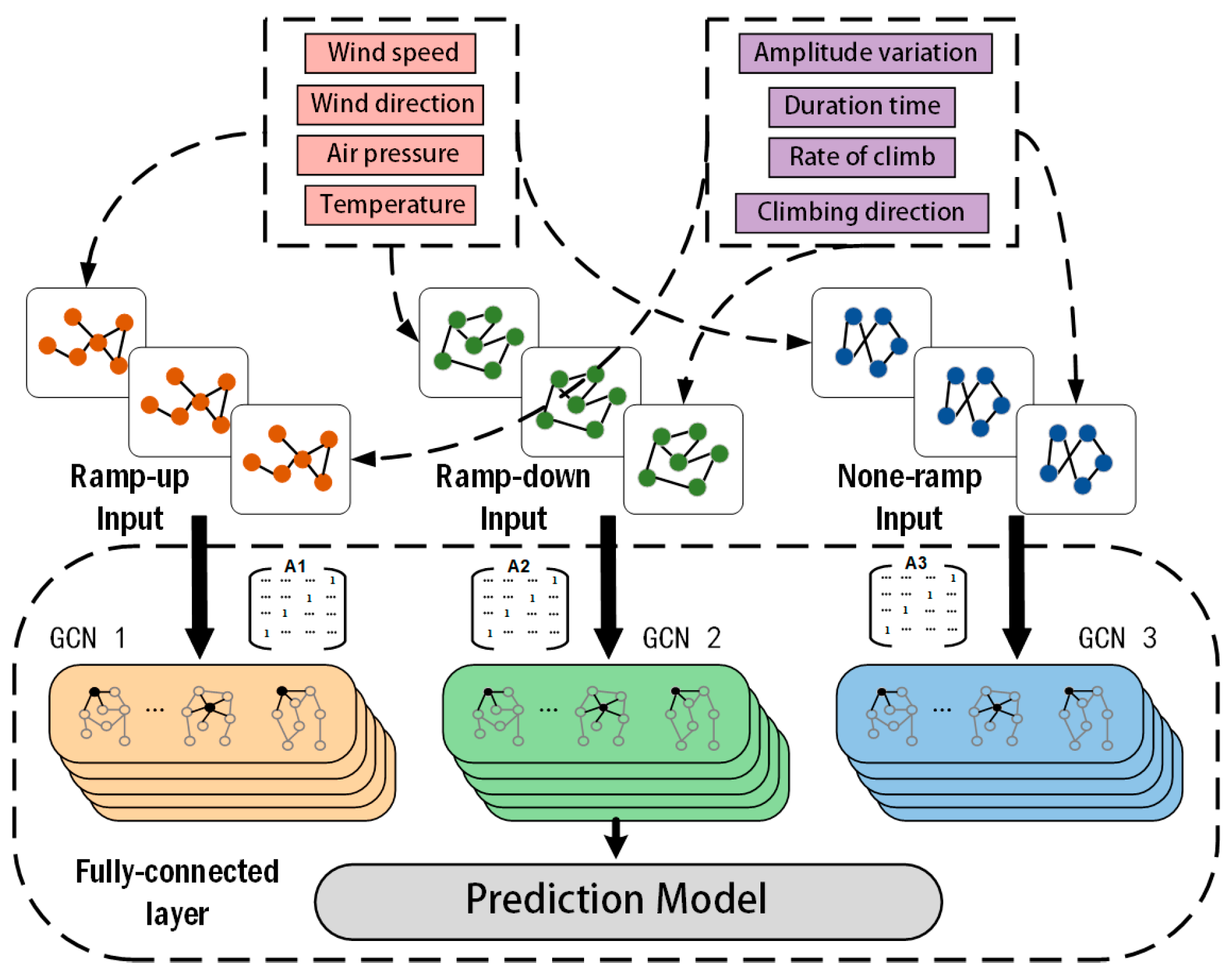
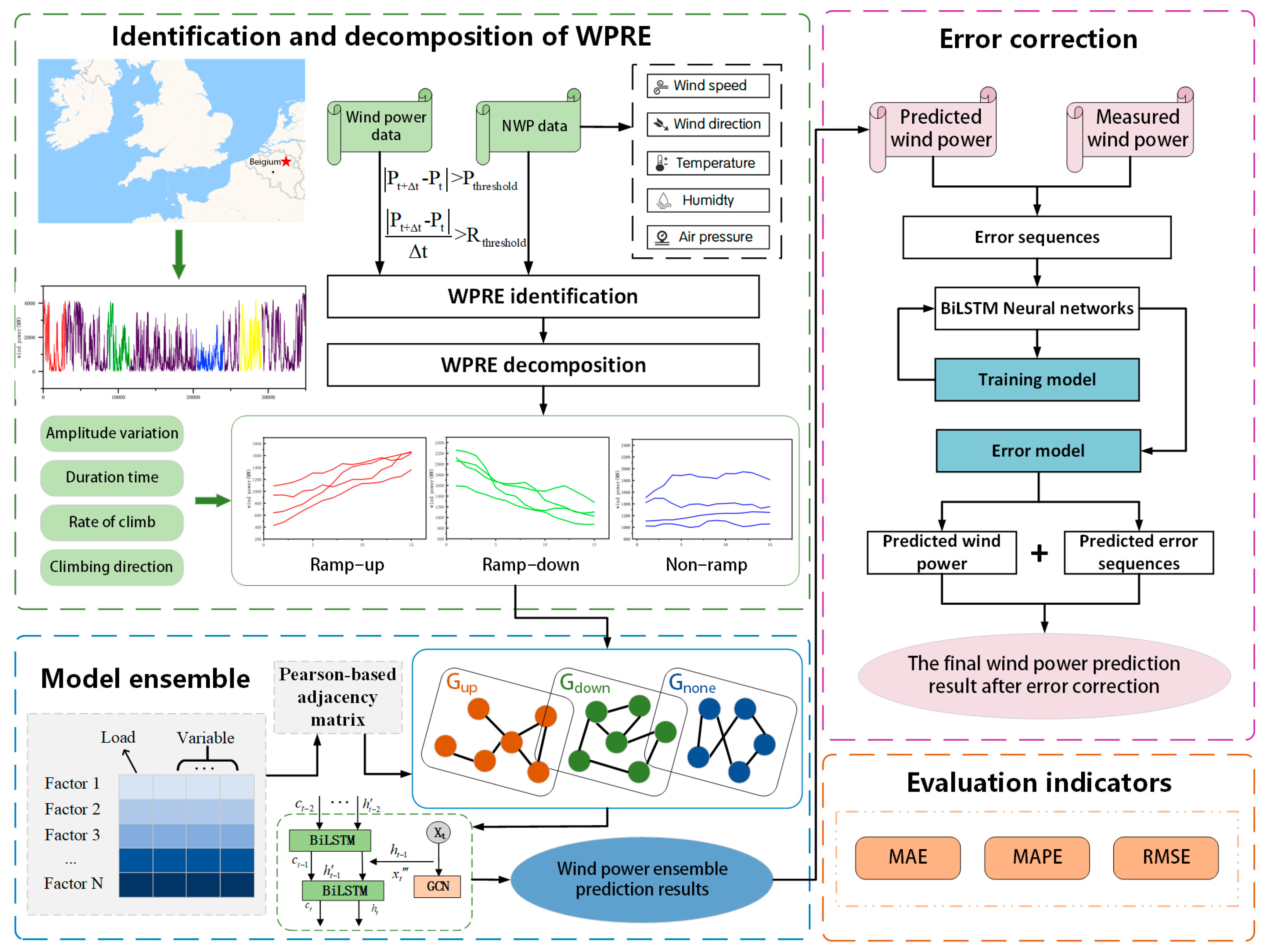
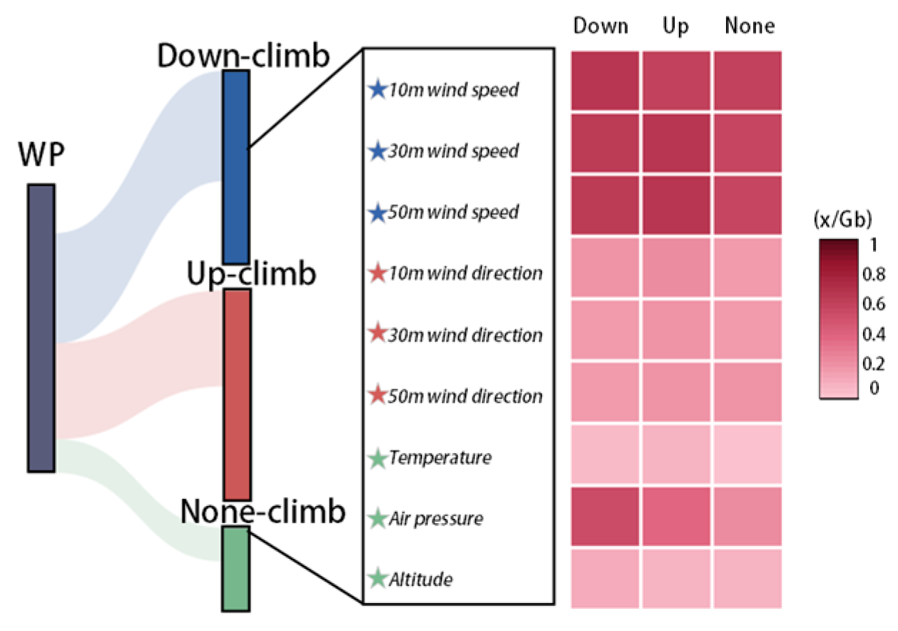
A novel ramp-aware graph neural network model is introduced. By performing Pearson correlation analysis, meteorological variables strongly correlated with distinct ramp phases are selected, and a multi-event feature graph is constructed to quantify the physical coupling characteristics of ramp events. The model then combines this graph representation with a BiLSTM network to enhance wind power forecasting accuracy.

(2)

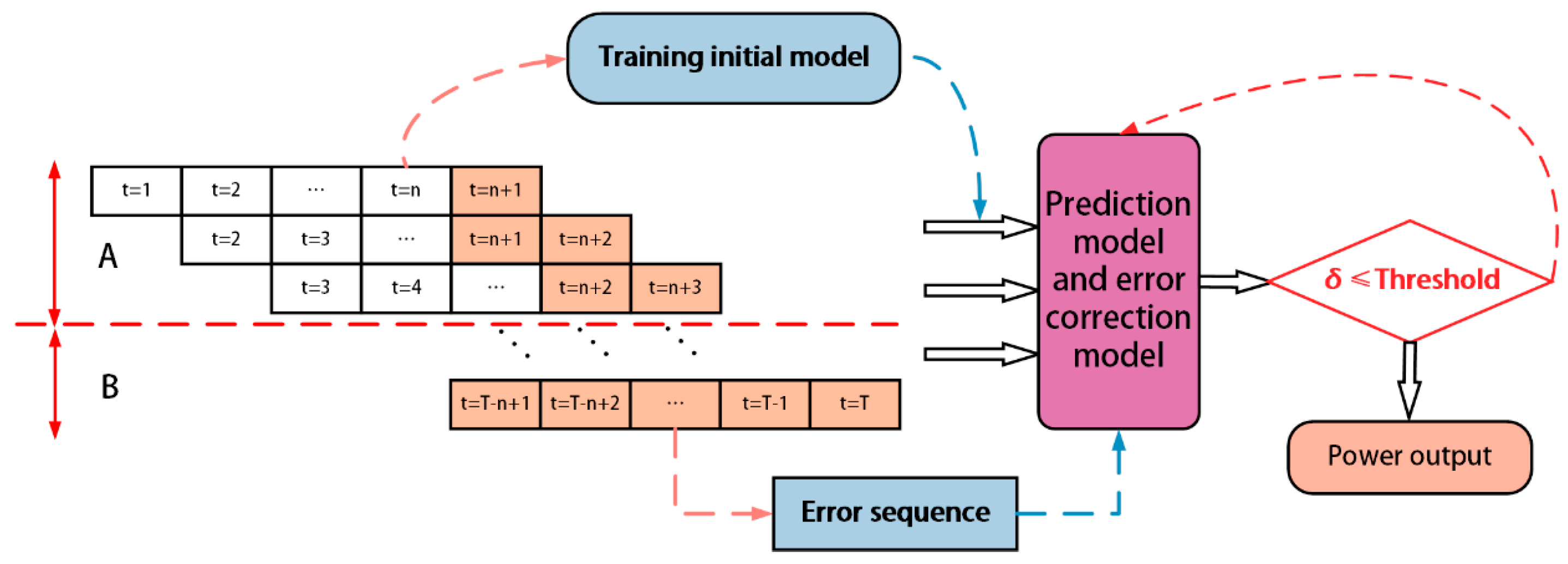
An error correction and dynamic feedback mechanism is developed. This module captures systematic prediction biases through error component modeling, providing a quantitative foundation for correction. It then performs dynamic adjustment of the power output in real time to continuously calibrate the forecasts.

The remainder of the paper is organized as follows: Section 2 outlines the methodological foundations of the proposed model; Section 3 presents the overall framework of the ramp-feature-aware graph neural network with integrated error correction; Section 4 analyzes results based on multiple datasets and compares the prediction performance across various methods; and Section 5 summarizes the findings and suggests directions for future work.

2. Correlation Method

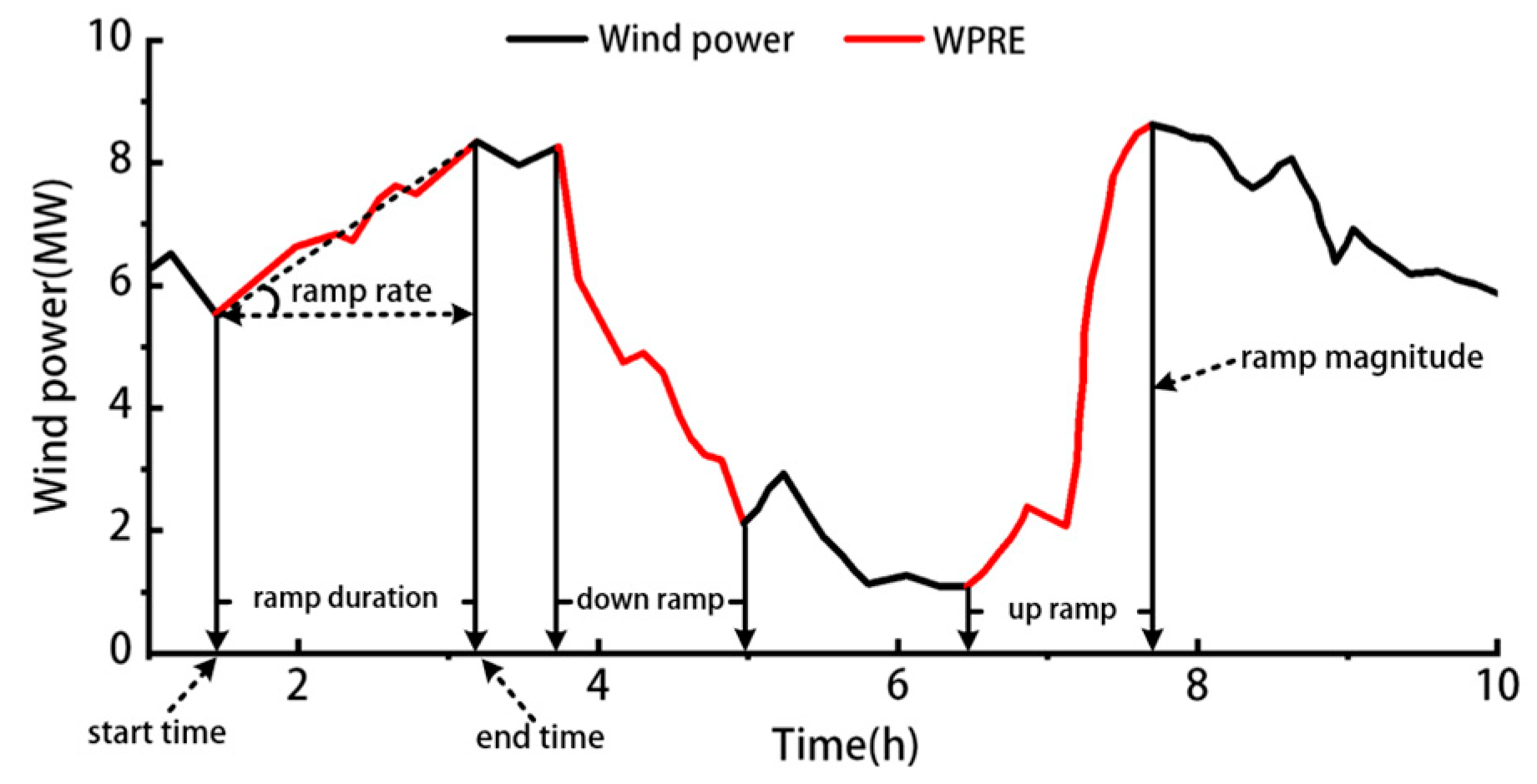
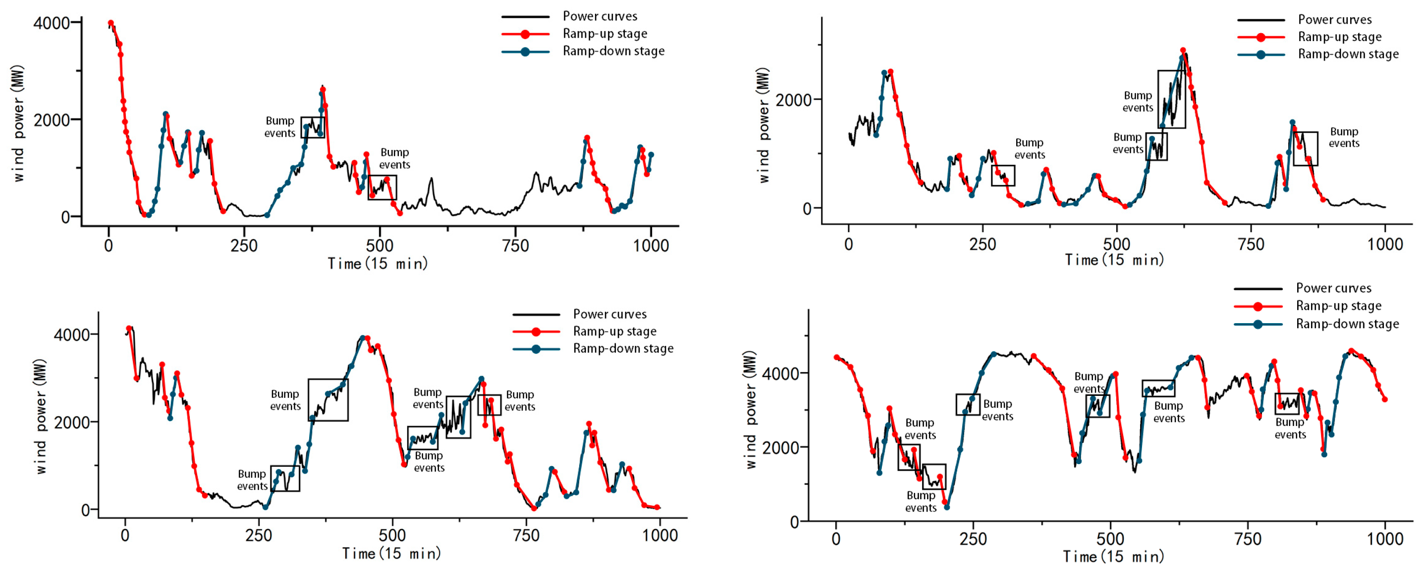
2.1. Definition of WPREs

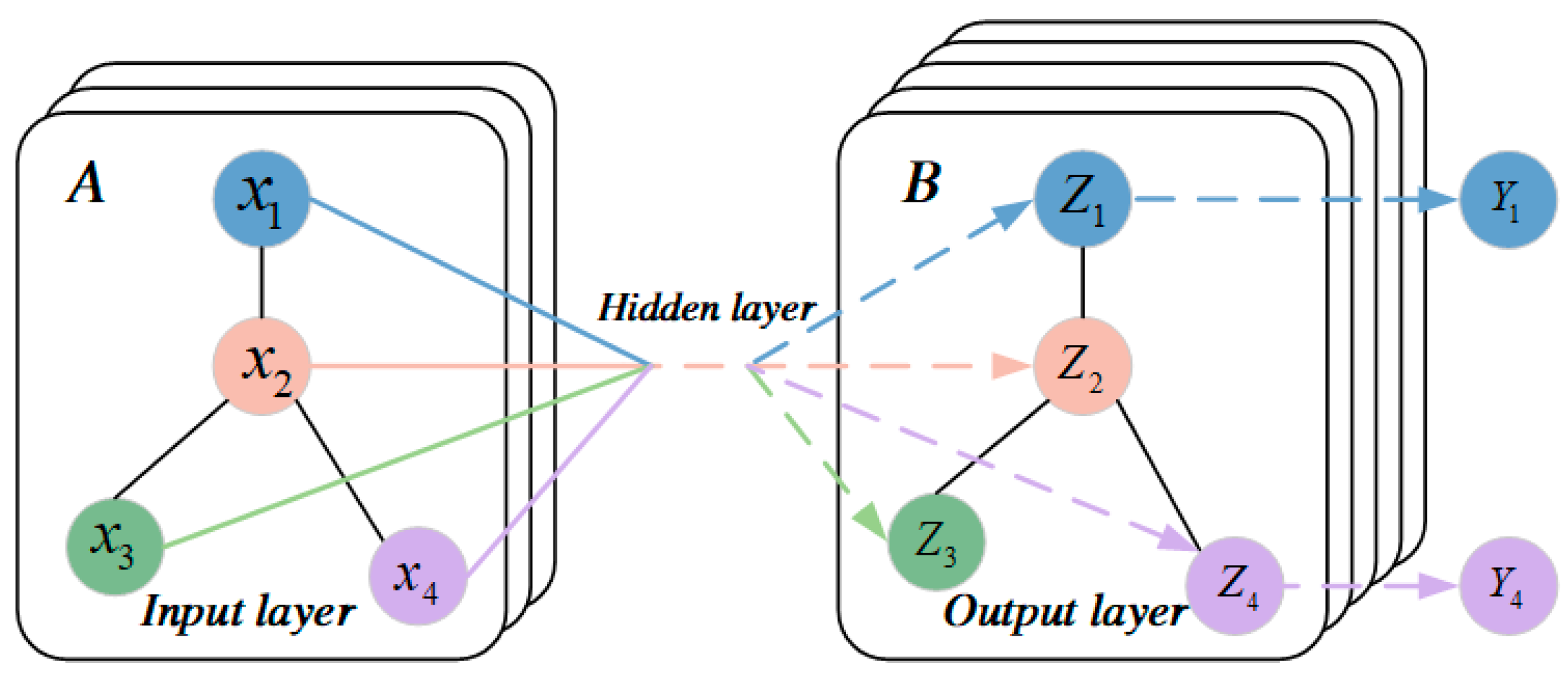
Grid security is multi-faceted and complex, and its security level cannot be characterized by a single indicator only, but needs to be described by multiple index simultaneously to reflect its overall level in a more comprehensive way. Therefore, this paper constructs a security evaluation index system with flexibility resource capacity index, flexibility resource response capability index, and branch load balance index to qualitatively and quantitatively reflect the security of the power grid.

As shown in Figure 1, WPREs have four characteristics [33,34,35], namely, the amplitude change $\Delta P_r$, duration $\Delta t$, ramp rate $\Delta P_r/\Delta t$, and ramp direction $D_r$, where $\Delta P_r$ is the change value of wind power in a certain period of time; $\Delta t$ is the duration when the wind power fluctuates greatly; $\Delta P_r/\Delta t$ is the change rate of wind power in a certain period of time; and $D_r$ is the wind power ramp direction within a certain period of time, including ramp-up, ramp-down, and non-ramp.

According to their four characteristics, WPREs are defined as follows.

Definition 1.

A ramp event occurs if the absolute value of the power difference between the start time and the end time in the time interval $(t,t+\Delta t)$ is greater than a given threshold, i.e.,

$$\left|P_{t+\Delta t}-P_t\right|>P_{threshold}$$

(1)

where $P_t$ and $P_{t+\Delta t}$ are the wind powers at the start time $t$ and the end time $t+\Delta t$, respectively, and $P_{threshold}$ is the threshold.

Definition 2.

A ramp event occurs if the ramp rate in the time period $(t,t+\Delta t)$ exceeds a given threshold, i.e.,

$${\displaystyle \frac{\left|P_{t+\Delta t}-P_t\right|}{\Delta t}}>R_{threshold}$$

(2)

where $R_{threshold}$ is the threshold of ramp rate.

Short-term and small fluctuations often exist in the wind power series. These small fluctuations will not affect the macro trend of wind power changes in time series but will affect the identification accuracy of WPREs. Therefore, in this paper, we adopt Definition 1 and Definition 2 to define the occurrence of WPREs [36]. Particularly, we will say a WPRE occurs if either condition (1) or (2) is satisfied. This can easily and succinctly eliminate the effect of bump events. Further, due to different ramp stages, we set 20% and 15% of the rated power as the ramp-up and ramp-down threshold, respectively, where the latter is slightly smaller than the former according to the standards found in the literature.

2.2. GCN Model

The Graph Convolutional Network (GCN) represents a convolutional neural network specifically designed for graph-structured data, initially proposed by Bruna in 2013 [37]. While conventional Convolutional Neural Network (CNN) excel at extracting spatial features from Euclidean structures, numerous non-Euclidean structures exist within power systems. GCN provides a novel approach for processing such data and has found extensive applications in power prediction, traffic forecasting, and related domains [38]. For a given graph $G$, input signal $X$, and output signal $Y$, the GCN processing method can be expressed as follows:

$$f\left(X,A\right)=Y$$

(3)

where $A$ denotes the adjacency matrix of the graph, with elements in matrix $A$ representing the connectivity relationships between nodes in graph $G$.

The propagation formula for graph convolution is expressed as follows:

$$H^{(l+1)}=\sigma \left({\tilde{D}}^{-1/2}\tilde{A}{\tilde{D}}^{-1/2}{H}^l{W}^l\right)$$

(4)

where $\tilde{A}=A+I$ represents the adjacency matrix with added self-connections ($l$ being the identity matrix); $\tilde{D}$ is the diagonal degree matrix; $H^l$ and $W^l$ denote the output and parameter values of the $l$ layer; and $\sigma (\cdot )$ represents the activation function.

The architecture of a multi-layer graph convolutional network is illustrated in Figure 2. The input layer receives graph data as signal $X$, and, through multiple GCN layers, the features of each node in the graph data are transformed from $X$ to $Z$, while the connectivity relationships $A$ between nodes remain unchanged. As wind power data can be decomposed into distinct ramp phases, utilizing graph neural networks for modeling and prediction can effectively capture different ramp characteristics, thereby enhancing prediction accuracy. Furthermore, since wind power output exhibits strong correlations with meteorological conditions, analyzing correlation factors across different ramp phases enables the division of wind power data into three distinct phases as described in Section 2.1: ramp-up phase, ramp-down phase, and non-ramp phase, allowing for the identification of different adjacency matrices for prediction purposes.

To more effectively extract wind power ramp characteristics and meteorological factor features, this study proposes an enhanced GCN architecture incorporating three specialized GCN modules. Each module is designed with distinct node configurations to characterize the dynamic coupling relationships between wind power ramp events and external meteorological conditions. The nodes are specifically categorized into wind power ramp characteristics and meteorological factor features, with inputs corresponding to different ramp phases and associated meteorological factors. The edge weights are computed using Pearson correlation coefficients, reflecting the linear association strength between nodes, and the construction of regular graph edges represents the inter-node correlations. Consequently, the expressions are modified as follows:

$$G_{up}=\sigma \left(\sum _{x=1}^L\left(\sum _{y=1}^V{\widehat{D}}^{-{\displaystyle \frac{1}{2}}}(i,i)\widehat{A}(i,y){\widehat{D}}^{-{\displaystyle \frac{1}{2}}}(y,y)P_{t-x+1}(y)\right)W(j,x)\right)$$

(5)

$$G_{down}=\sigma \left(\sum _{x=1}^L\left(\sum _{y=1}^{\nu }{\widehat{D}}^{-{\displaystyle \frac{1}{2}}}(i,i)\widehat{A}(i,y){\widehat{D}}^{-{\displaystyle \frac{1}{2}}}(y,y)W{S}_{t+x}(y)\right)W(j,x)\right)$$

(6)

$$G_{none}=\sigma \left(\sum _{x=1}^L\left(\sum _{y=1}^{\nu }{\widehat{D}}^{-{\displaystyle \frac{1}{2}}}(i,i)\widehat{A}(i,y){\widehat{D}}^{-{\displaystyle \frac{1}{2}}}(y,y)W{S}_{t+x}(y)\right)W(j,x)\right)$$

(7)

$$w_{ij}={\displaystyle \frac{\mathrm{cov}(v_i,v_j)}{{\sigma }_{v_i}{\sigma }_{v_j}}}$$

(8)

where $G_{up}$, $G_{down}$, and $G_{none}$ represent the GCN models for ramp-up, ramp-down and non-ramp phase characteristics, respectively. $L$ denotes the extracted time series length, $v$ represents the meteorological factor sequence, $A$ is utilized for adjusting ramp characteristics and fluctuation correlations, and $W$ is employed for extracting temporal features. The threshold $w_{ij}$ retains edges with $\left|w_{ij}\right|>0.5$, eliminating low-correlation connections to reduce noise. Through refined node and edge design, the physical mechanisms of wind power ramp events are encoded as explicit associations in the graph layers, enabling the graph neural network to more accurately model the characteristic dependencies of power fluctuations. The architecture of the proposed GCN model is illustrated in Figure 3.

2.3. BiLSTM Model

As an improved recurrent neural network, the BiLSTM model can take into account the influence of both historical and future data information on prediction accuracy [39]. By using a bidirectional model, it incorporates data information both before and after the prediction point into the prediction process, which is more in line with the changing trends and patterns of wind power.

The BiLSTM model is as follows:

$$\overrightarrow{h_t}=L_1(h_{t-1},i_t,c_{t-1}),t=1,2,\dots ,n,$$

(9)

$$\overleftarrow{h_t}=L_2(h_{t+1},i_t,c_{t+1}),t=1,2,\dots ,n,$$

(10)

$$B_t=a_t\overrightarrow{h_t}+b_t\overleftarrow{h_t}+c_t,t=1,2,\dots ,n,$$

(11)

where $\overrightarrow{h_t}$ and $\overleftarrow{h_t}$ are the forward and backward output of the hidden layer, respectively; $L_1$ and $L_2$ are the forward and backward calculation process in the LSTM network model, respectively; $h_t$ is the predicted value at time $t$; $c_t$ is the bias optimization parameter at time $t$; $a_t$ and $b_t$ are the output weights; $i_t$ is the input of the LSTM model at time $t$; and $B_t$ is the final output of the LSTM network.

2.4. Error Correction Model

To address the limitation of existing prediction models that primarily rely on raw data predictions while inadequately accounting for forecast errors between predicted and actual values, this study proposes a dynamic error correction model based on historical power data [40]. The developed framework enhances conventional wind power prediction models by integrating an error forecasting component, which directly captures intrinsic relationships between predicted and true power outputs without assuming error distributions. Through systematic modeling and closed-loop feedback mechanisms, this approach achieves progressive accuracy improvement, as illustrated in Figure 4.

The proposed methodology comprises three key phases. First, the training dataset is divided into two subsets: Subset A is used to train the initial prediction model, enabling it to learn global patterns from the power sequences; Subset B is utilized to generate forecasts from the trained model, which are then compared with actual measurements to construct a non-stationary error sequence. In the second phase, the initial prediction model is combined with the error correction module. Historical wind power data are used to produce baseline predictions, which are subsequently refined by adding error estimates generated by the correction model, yielding the final corrected outputs. In the final phase, a closed-loop feedback mechanism is introduced to address distributional drift. When the corrected residuals consistently exceed a predefined threshold, the system initiates incremental updates to the error correction model. This adaptive process enables the framework to dynamically respond to the non-stationary characteristics of wind power data by progressively incorporating test samples into the training set.

The mathematical formulation of the error correction model is defined as follows:

$$e=y-y^{\prime }$$

(12)

$$e^{\prime }(t)=f\left[e(t-T),e(t-2T),\dots ,e(t-nT)\right]$$

(13)

$$y^{″}=y^{\prime }+e^{\prime }$$

(14)

$$r_t=y^{″}-y$$

(15)

$${\displaystyle \frac{1}{w}}{\displaystyle \sum _{i=t-w+1}^t\frac{r_i}{y_i}}>\theta$$

(16)

where $y$ and $y^{\prime }$ are the actual value and initial predicted value of wind power, respectively; $e$ is the predicted error series; $e(t-nT)$ is the $n\mathrm{t}\mathrm{h}$ historical prediction error before time $t$; and $y^{″}$ is the final predicted value of wind power after the error correction. $r_t$ is the defined residual, $w$ is a set sliding window, and every certain period of time (sliding window), the error between the corrected predicted value and the true value is calculated to see if it continues to be too large. Once the error is found to continue to exceed, the data of this period of time is used as a new training sample to update the error correction result.

3. Short-Term Prediction Based on WPREs Recognition and GCN

3.1. Basic Idea of Forecasting

This study presents a wind power forecasting approach that integrates ramp feature identification and error correction within a graph neural network framework. As shown in Figure 5, the overall prediction architecture consists of three stages, each corresponding to a specific methodological component. In the first stage, historical wind power sequences are analyzed for ramp events through correlation analysis with relevant meteorological variables. Based on this analysis, the sequences are classified into three categories: upward-ramp, downward-ramp, and non-ramp phases. In the second stage, multi-event graph structures are constructed to capture the complex correlations among different ramp segments. These graphs serve as the basis for generating the initial prediction results. In the final stage, a dynamic feedback-based error correction model is applied to refine the preliminary forecasts, producing the final wind power prediction output.

As mentioned above, different graph networks are constructed for different segments, and the differences between each segment can be fully taken into account. This integrated prediction model can accurately predict wind power data, thus improving the prediction effect of the model.

3.2. Prediction and Evaluation Index

The importance of wind power prediction algorithms largely relies on the accuracy of their predictions. Greater accuracy in prediction results leads to increased guidance value for power systems. To objectively assess the accuracy of prediction results, it is essential to establish evaluation indicators that verify the feasibility and effectiveness of the proposed method and allow for comparison between different algorithms’ prediction outcomes.

Let $y_b=(y_1,y_2,\dots ,y_B)$ and $y_{c,b}=(y_{c,1},y_{c,2},\dots ,y_{c,B})$ be the actual values and predicted ones of wind power, respectively, and $B$ be the length of the predicted sequence. Then, we define the following evaluation indicators:

The root mean square error (RMSE):

$$RMSE=\sqrt{{\displaystyle \frac{1}{B}}{\displaystyle \sum _{b=1}^B{(y_{c,b}-y_b)}^2};}$$

(17)

The average absolute error (MAE):

$$MAE={\displaystyle \frac{1}{B}}{\displaystyle \sum _{b=1}^B\left|\frac{y_{c,b}-y_b}{y_b}\right|}$$

(18)

The average absolute percentage error (MAPE):

$$MAPE={\displaystyle \frac{100\%}{n}}{\displaystyle \sum _{b=1}^B\left|\frac{y_{c,b}-y_b}{y_b}\right|}$$

(19)

3.3. Data Preprocessing

(1)

Missing value supplementation

When there are missing data in the wind power dataset, the uncertainty of wind power will be aggravated. Therefore, it is necessary to fill in the missing data. Time series correlation can be used for interpolation, mainly by integrating adjacent time period data or historical data of the same period to supplement missing values. This paper considers the periodic law of wind power and selects the historical data with the strongest correlation 24 h before and after the target time to construct an interpolation supplement model. The calculation principle is mainly shown in the following formula:

$$p(t)={\displaystyle \frac{1}{2}}(p(t-24)+p(t+24))$$

(20)

where $p(t)$ is the wind power value to be filled at time t; $p(t-24)$ is the power value at the same time in the previous 24 h; $p(t+24)$ is the power value at the same time in the next 24 h.

(2)

Outlier correction

The wind power data acquisition system may generate some invalid data during the collection and sorting process, such as null values and negative values. For these invalid data, this section will use a rolling detection mechanism to clean the data. For the identified and screened abnormal data points, they will be deleted and replaced by data points at other times. The replacement method used in this section is similar to the processing method of missing value supplementation. The effective power value at the adjacent time of the abnormal data point is selected for data replacement:

$$p(t)={\displaystyle \frac{1}{2}}(p(t-1)+p(t+1))$$

(21)

where $p(t)$ is the abnormal data point to be corrected, which will be deleted and replaced; $p(t-1)$ is the wind power value of the adjacent time node before the target data point; $p(t+1)$ is the wind power value of the adjacent time node after the target data point.

4. Case Analysis

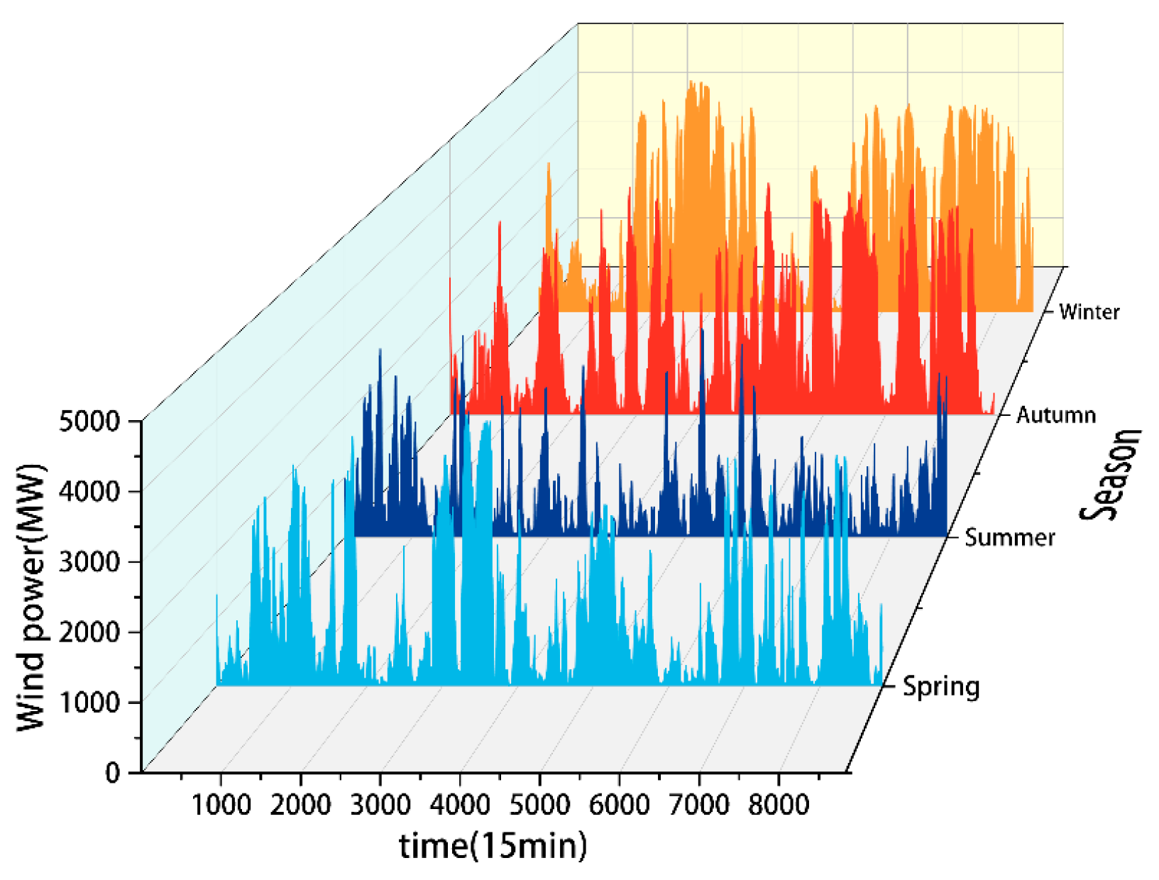
4.1. Original Dataset Description

The wind power sample data used in this paper is sourced from a Belgian wind farm obtained on the Elia website. The data have a sampling interval of 15 min, and the wind farm has an installed capacity of 5041.047 MW. Belgium’s climate, geographical location, and wind energy resources are representative of European conditions. The wind farm’s location is influenced by the Atlantic airflow, with changes in wind speed and direction effectively reflecting the wind farm’s operation across various seasons and weather conditions. Consequently, this dataset is beneficial for the effective analysis and research of the prediction method proposed in this paper.

Given that wind power is significantly influenced by seasonal and weather characteristics, we utilize data from the entire year of 2022 as the research sample, dividing it into four quarters. Figure 6 displays the original wind power data of the Belgian wind farm for 2022. To demonstrate the impact of different power fluctuation frequencies and amplitudes on the proposed model, January, April, August, and October are chosen as representative months across the four seasons for analysis. In each of these months, 1000 sample data points are selected for case analysis, with the first 50% used as the training set and the remaining 50% as the test set. Although the 70/30 or 80/20 split is more commonly used in machine learning, this setting was chosen for the following reasons: first, the ramp decomposition process reduced data redundancy and produced balanced subsequences across ramp types, ensuring sufficient samples even with a reduced training portion. Second, by enlarging the test set, we aimed to provide a more robust assessment of the model’s predictive accuracy, particularly under less frequent but highly volatile ramp events, which are the primary focus of this study. The 50/50 setting offered a more balanced and representative evaluation across all ramp phases.

Altering the number of model inputs can enhance prediction accuracy. This paper evaluates the performance of the proposed model using 1-step ahead, 2-step ahead, and 3-step ahead prediction strategies, verifying the effectiveness of this method through a multi-step prediction mechanism.

This paper will use the graph convolutional network prediction method considering ramp events to predict wind power. The model is simulated in Python 3.9 language, and the optimal structure of the model is determined by the control variable method. The model is tested and trained using the training set, and the first 9 power sampling points are used to predict the next power point. The number of GCN layers is designed to be two, and different structures are adopted for different ramp event adjacency matrices. By adjusting the parameters, the best effect is achieved when the initial learning rate is 0.001, the initial training round is 100 times, the BiLSTM is two layers, the batch size is 64, and the Dropout is 0.2–0.3.

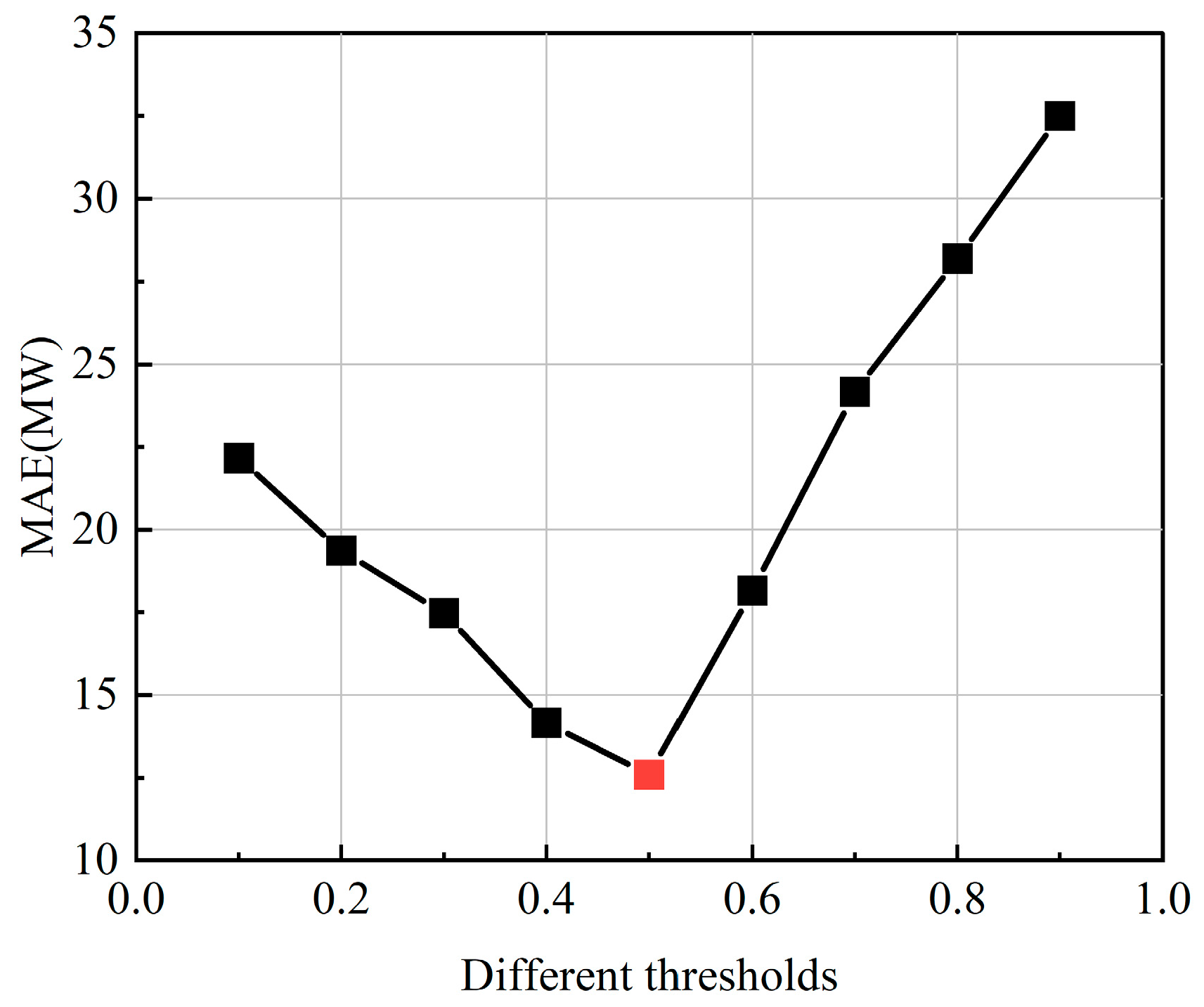
4.2. Calculation of Scheduling Time Period Weights and Indicator Weights

Taking the wind power data of four typical months in the four seasons of 2022 at the Elia website’s Belgian wind farm as an example, a comprehensively improved ramp definition is proposed, and the basic wind power sequence is decomposed into an ramp-up, ramp-down, and non-ramp stages. Figure 7 shows the wind power sequence after ramp decomposition.

The results of ramp events are shown in

Table 1. Analysis table of WPREs in four seasons.

	Spring	Summer	Autumn	Winter
Ramp-up event	9	12	12	11
Ramp-down event	8	11	11	13
Non-ramp event	3	4	2	2

. Obviously, in autumn and winter, due to windy and rainy weather, there are more cases of rapid changes in wind power, and bump events are more common, while in spring and summer, due to mostly sunny weather, the wind power is in a gentle stage, and only in a few cases will there be rapid power changes. Therefore, eliminating the impact of bump events and predicting wind power in all four seasons at the same time will help improve data quality and analyze the impact of different numbers of ramp events on the graph neural network prediction model proposed in this paper.

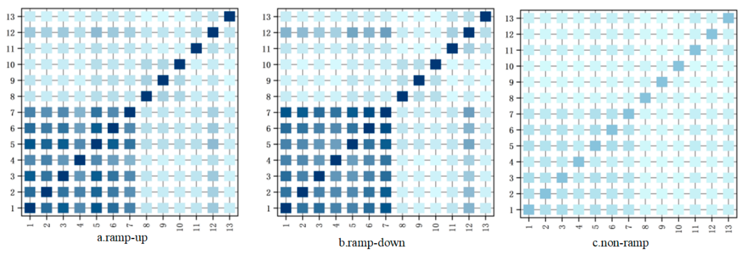
4.3. GCN Node Analysis

According to the aforementioned introduction, the NWP data for the wind farm encompasses wind speed measurements at tower heights of 10, 30, and 50 m, as well as wind direction at these same heights. Additionally, it includes meteorological parameters such as temperature, air pressure, and humidity. The climbing characteristics of wind power are defined by amplitude variation, duration, climbing rate, and climbing direction. Utilizing the known numerical weather forecast sequences, Pearson correlation analysis is conducted to investigate the intrinsic relationships between meteorological factors and various climbing sequences. The results of the correlation heat map analysis are presented in Figure 8.

By analyzing Figure 8 and comparing the correlation coefficients between the power and meteorological characteristics of different climbing sections, the following conclusions can be drawn: (1) The correlation coefficients between the wind speed at 10 m, 30 m, and 50 m and the power of each climbing section are all around 0.8, indicating that wind speed is the most important factor affecting power. (2) The correlation coefficients between the wind direction at 10 m, 30 m, and 50 m and the power of each climbing section are all around 0.25, and the wind direction has only a certain correlation with the output power. (3) The correlation between air pressure, temperature, and humidity and the power of each climbing section is slightly different. The rapid drop in air pressure gradient will also cause power to climb down, so the correlation between air pressure and the downhill section is the highest, followed by the uphill and non-climbing sections. Combining the results of the correlation analysis, the three adjacency matrices shown in Figure 9 are obtained. The matrices are sparse and diverse in nature. Each matrix carries different information and complements each other to form a complete feature association system. This prediction model provides more comprehensive information.

The adjacency matrix characterizes the association pattern between different climbing sections and meteorological factors, providing an explicit topological structure for GCN. At the same time, the graph structure is independently constructed for different climbing events to avoid confusion of feature association patterns. In the up-climbing event: low-altitude wind speed (10 m, 30 m) and climbing characteristics (amplitude change, climbing rate) show a strong correlation, indicating that low-altitude wind shear has a significant driving effect on the rapid increase in power; the change in pressure gradient further verifies the impact of meteorological system dynamics on the up-climbing event. In the down-climbing event: the high-altitude wind speed (50 m) has the highest correlation with the power drop, reflecting the physical law of the high wind speed cut-out mechanism; at the same time, the strong pressure gradient indicates that the sudden change in air pressure is an important environmental factor triggering the power drop. In the non-climbing event: the correlation between temperature and humidity is dominant, while the influence of wind speed and wind direction is weak, which is consistent with the characteristic of small power fluctuations under stable meteorological conditions. Through multi-layer message passing, GNN can further extract nonlinear information from weakly correlated features such as wind direction and humidity, making up for the limitation of the Pearson correlation coefficient that only measures linear relationships, enhancing the interpretability of the graph structure and laying a solid foundation for subsequent predictions.

Based on the above analysis of the correlation between wind power ramp events and meteorological factors, the threshold will be selected below. Different thresholds are set, and the ramp characteristics and influencing factors with correlation index greater than the threshold are input into the prediction model from high to low. In the preliminary comparison, we observed that a lower threshold will produce an overly dense graph, thereby reducing the prediction accuracy, while a higher threshold will lead to graph fragmentation and insufficient connectivity. The relationship between threshold selection and MAE value is shown in Figure 10. It can be seen from the figure that when the threshold is selected as 0.5, the MAE is the smallest; therefore, the error is the smallest.

4.4. Predictive Model Results Analysis

In this subsection, we utilize the prediction method of ramp feature recognition to forecast wind power. The proposed method’s effectiveness is validated by comparing it with prediction methods from other sources.

To verify the predictive efficacy of the proposed method, we compared the data predicted by the BiLSTM method (Model 1) and the GCN method (Model 2) to those predicted by the proposed method (Model 3) evaluating by previously defined evaluation indicators: RMSE, MAE, and MAPE.

To validate the effectiveness of the proposed forecasting model, this study designs wind power prediction experiments from two perspectives: (1) comparative performance evaluation between the graph neural network prediction model incorporating ramp feature recognition and benchmark models without ramp feature consideration on identical wind power datasets; (2) systematic investigation of various models across multiple forecasting horizons and seasonal variations in wind power sequence prediction. This dual-strategy experimental design ensures comprehensive assessment of model robustness and generalization capability under diverse operational scenarios. Figure 11, Figure 12, Figure 13 and Figure 14 clearly display the predicted output results under various scenarios.

Table 2. The wind power prediction error results before and after ramp feature recognition.

	Index	Spring			Summer			Autumn			Winter
Method		MAE	MAPE	RMSE	MAE	MAPE	RMSE	MAE	MAPE	RMSE	MAE	MAPE	RMSE
Before		30.066	0.128	38.965	39.666	0.128	70.922	65.134	0.108	91.625	65.768	0.022	94.946
After		12.597	0.051	17.690	23.506	0.068	40.483	29.304	0.052	52.756	42.067	0.014	59.691

and

Table 3. Error comparison of several prediction models at different prediction steps.

Season	Step	Evaluation Indicators	Model 1	Model 2	Model 3
Spring	1-step ahead	MAE	22.869	27.127	15.1713
		MAPE	0.0836	0.1756	0.0595
		RMSE	32.1357	33.843	21.9507
	2-step ahead	MAE	21.9859	25.93	21.3648
		MAPE	0.0789	0.0929	0.0786
		RMSE	30.8346	36.0336	29.7885
	3-step ahead	MAE	22.8793	22.3461	22.214
		MAPE	0.0785	0.089	0.0781
		RMSE	32.2695	31.6698	30.7075
Summer	1-step ahead	MAE	39.6276	36.1062	19.0921
		MAPE	0.1712	0.1237	0.0693
		RMSE	71.8246	68.3593	32.8247
	2-step ahead	MAE	38.7775	34.8332	23.9008
		MAPE	0.1543	0.0804	0.0745
		RMSE	72.0189	68.0761	40.4538
	3-step ahead	MAE	40.4744	38.2804	26.6685
		MAPE	0.2226	0.1278	0.0984
		RMSE	72.5032	69.5466	44.9899
Autumn	1-step ahead	MAE	56.7392	51.3428	50.7459
		MAPE	0.1002	0.0663	0.0591
		RMSE	87.0996	78.8623	79.7704
	2-step ahead	MAE	55.7436	51.863	51.9949
		MAPE	0.1052	0.0704	0.079
		RMSE	83.9547	79.9794	80.7358
	3-step ahead	MAE	55.4655	52.0087	49.404
		MAPE	0.1133	0.1045	0.078
		RMSE	83.3012	78.4778	76.3651
Winner	1-step ahead	MAE	66.7616	62.837	55.5984
		MAPE	0.0223	0.021	0.0157
		RMSE	95.7773	90.7758	81.2365
	2-step ahead	MAE	71.1707	57.9993	58.812
		MAPE	0.0235	0.0196	0.019
		RMSE	98.3987	84.1629	83.2265
	3-step ahead	MAE	66.0338	62.7856	60.1348
		MAPE	0.0221	0.021	0.0194
		RMSE	94.2949	89.9361	84.1961

present the prediction errors of different scenarios and prediction models. Figure 15, Figure 16 and Figure 17 illustrate the prediction error distribution of different scenarios and prediction models. Based on these results, we will analyze the predictive performance of the model from two perspectives: results with the recognition of ramp features and results with multi-step prediction.

(1)

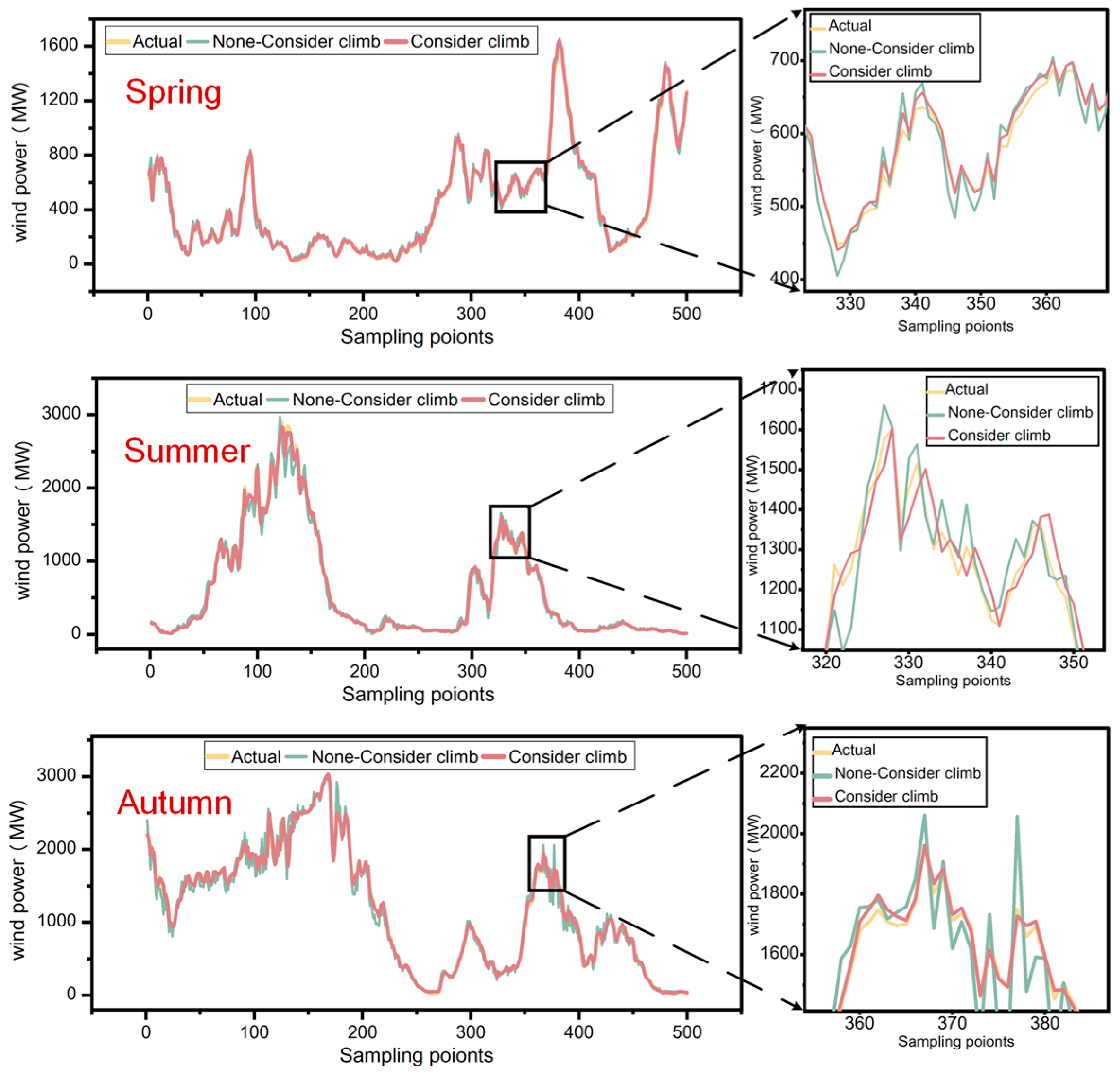
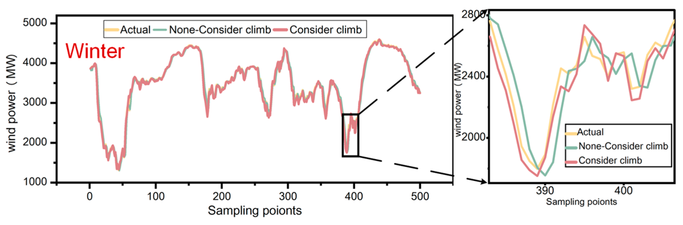
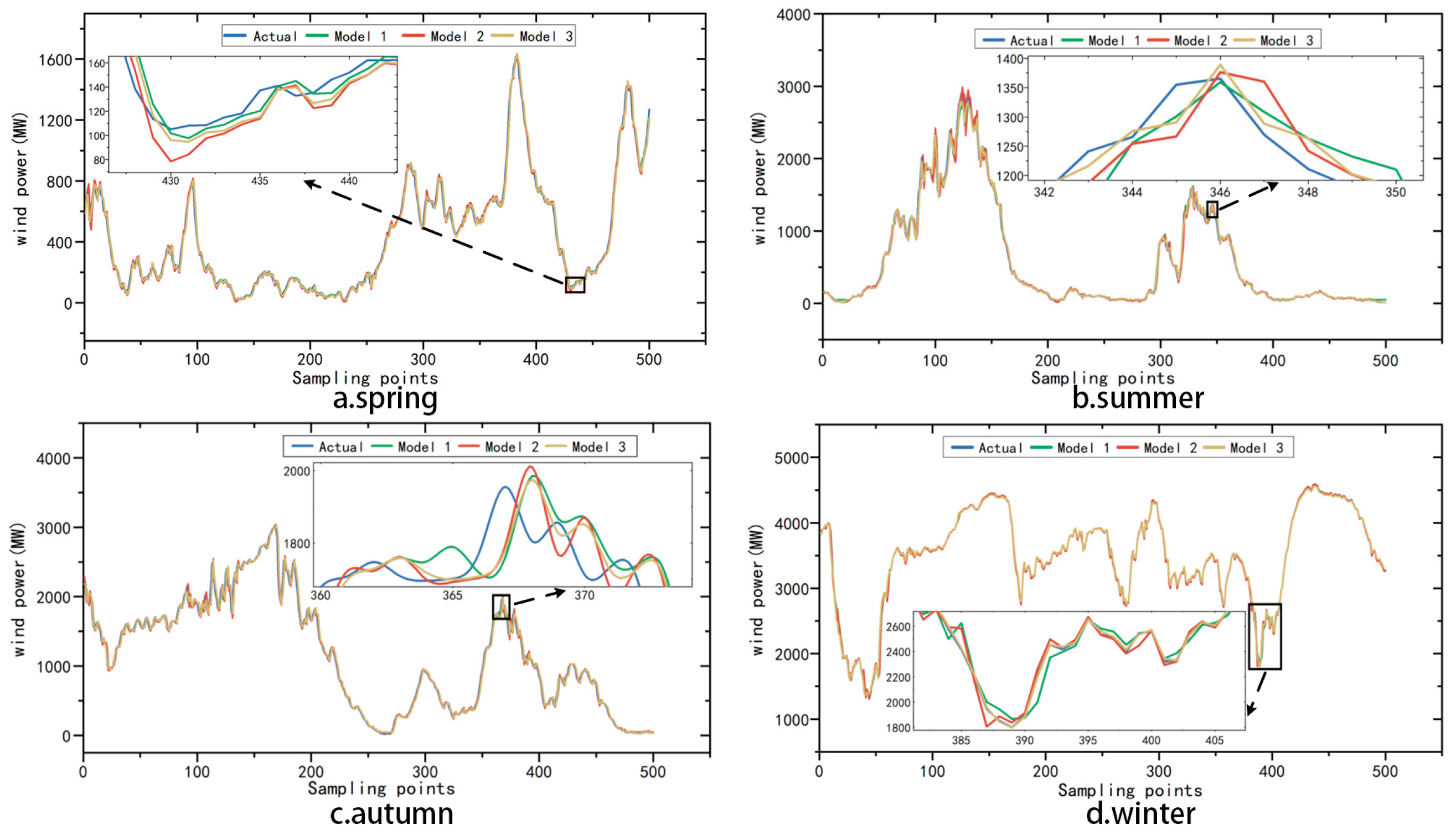
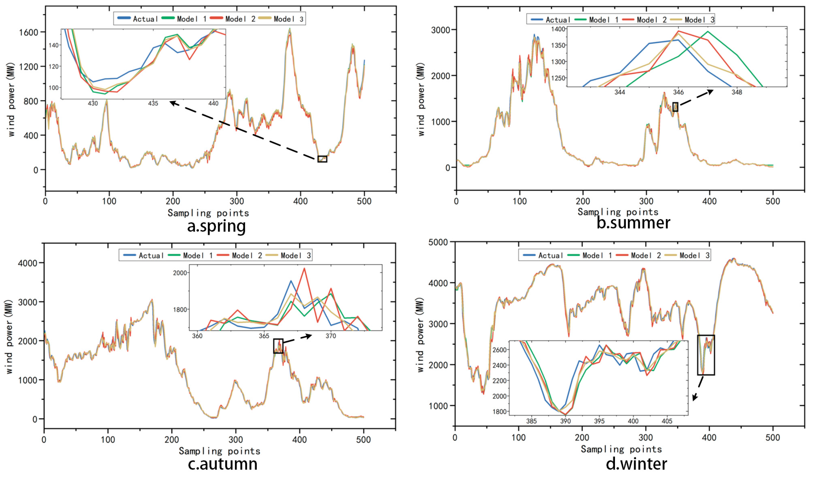
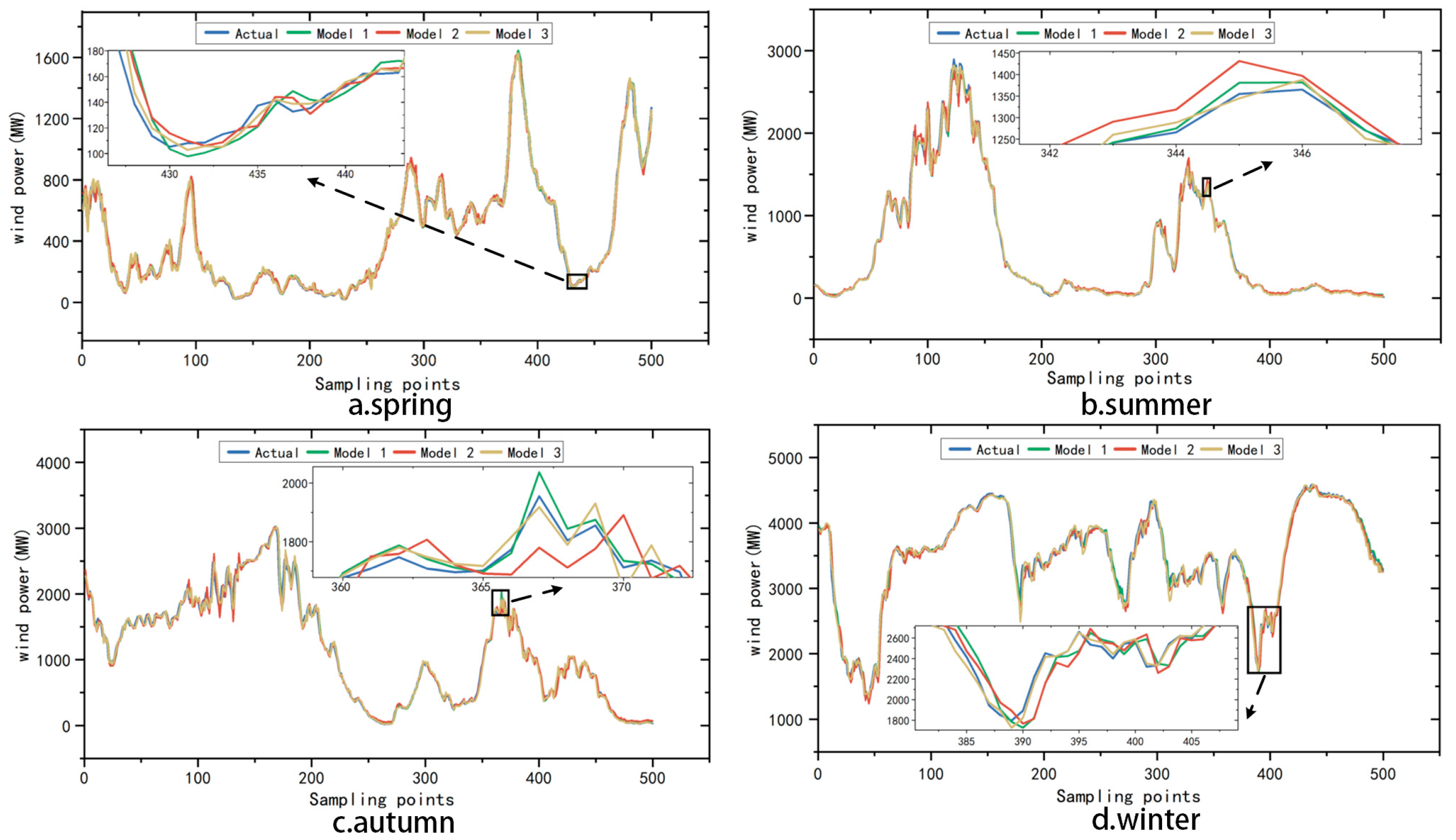
Analysis of the prediction results considering the recognition of ramp features

As Figure 11 clearly demonstrates, in spring, summer, autumn, and winter, the prediction model considering ramp feature recognition offers distinct advantages, whether comparing the actual wind power value or tracking the wind power change trend. The prediction graphs for the four seasons are partially enlarged, and it can be seen that: when the climbing characteristics are not considered, the model’s prediction ability for wind power is poor, and large errors will occur in the range of drastic fluctuations; after considering the climbing characteristics, the predicted value of wind power is more closely aligned with the true value, and can better track the changing trend of wind power. The integrated forecasting method proposed in this paper effectively follows the fluctuation trend of wind power under varying fluctuation frequencies and sizes, demonstrating high accuracy. Though the prediction model that does not consider ramp feature recognition can track wind power changes to some degree, the trend is not as prominent, and its performance is inferior in some seasons, falling short of the method proposed in this paper. Overall, the integrated prediction model proposed in this paper more effectively tracks the trend change in wind power under different fluctuation frequencies and sizes (across different seasons).

A comprehensive comparison of different seasons and corresponding error indicators is presented in Table 2. After considering the recognition of ramp features and comparing the error indexes of the integrated prediction model with those without considering ramp feature recognition, the MAE, MAPE, and RMSE decreased significantly. In the spring prediction results, MAE, MAPE, and RMSE decreased by 58.10%, 60.56%, and 54.60%, respectively. In summer, these values decreased by 40.74%, 46.96%, and 42.92%, respectively. In autumn and winter, the error indexes also decreased by more than 20%, proving the effectiveness of the prediction model considering ramp feature recognition.

To account for the above error results, two fitting curves are included in each panel of Figure 13 to assess the overall accuracy of the model. From the scatter plot, we can see that regardless of the season, the prediction results without considering the climbing characteristics are quite divergent. In spring, the actual values diverge more severely in the range of 750–1000, in summer, the actual values diverge more severely in the range of 2000–3000, in autumn, the actual values diverge more severely in the range of 1000–3000, and in winter, the actual values diverge more severely in the range of 1000–3000. It is evident that the integrated prediction model considering ramp feature recognition has the best prediction effect, outperforming the model without considering ramp feature recognition. To further compare the influence of different forecasting steps on the prediction results, the prediction outcomes and evaluation indicators under various forecasting compensations are statistically analyzed.

(2)

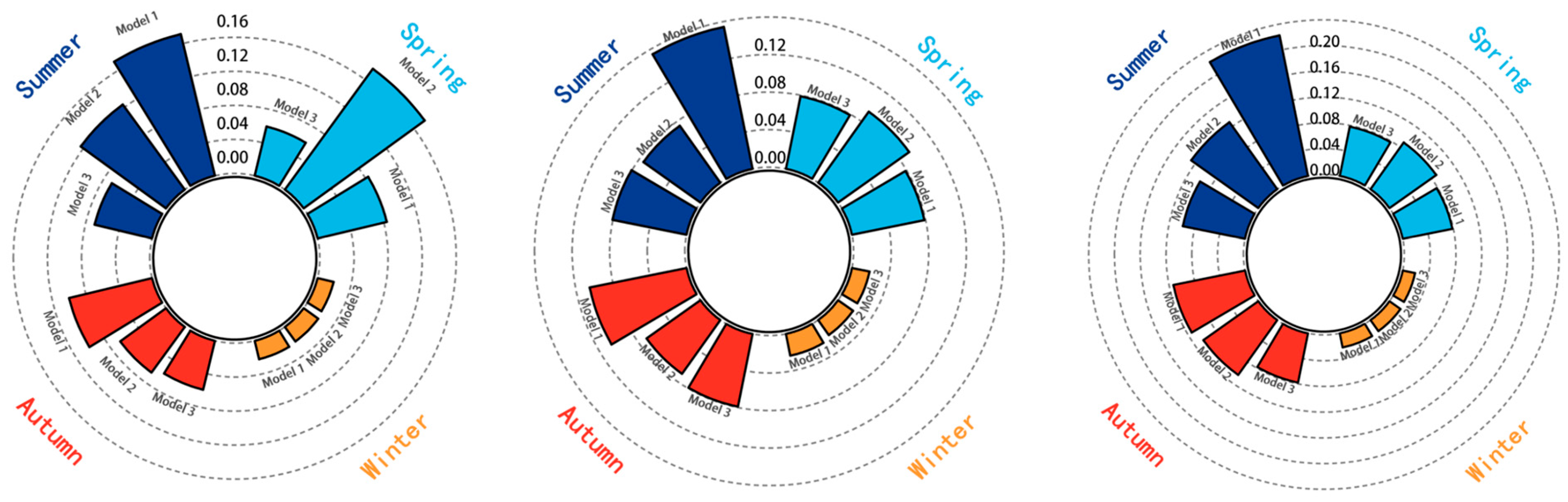
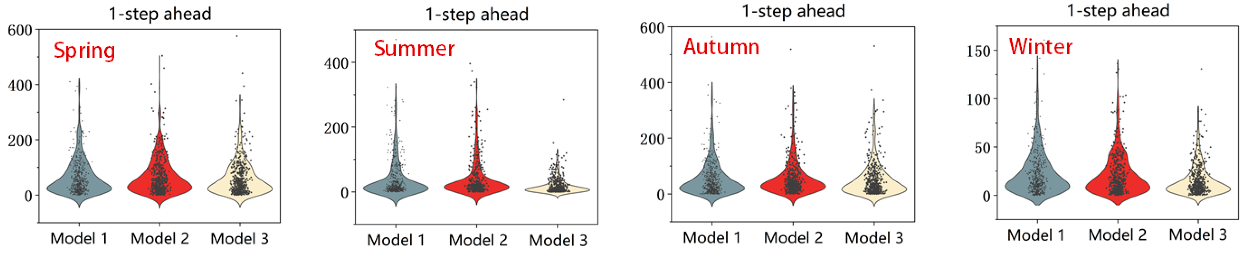
Analysis of the prediction results with multi-step prediction

To acquire more detailed information on future wind power prediction, multi-step wind power prediction is useful. In order to verify the performance of the prediction model proposed in this paper for multi-step advance prediction, one to three step advance predictions were carried out for wind power series. Figure 12, Figure 13 and Figure 14 display the results of 1-step, 2-step, and 3-step ahead predictions under different seasons.

It can be seen from Figure 12, Figure 13 and Figure 14 that the prediction accuracy decreases as the prediction step length increases. According to Figure 12a, Figure 14a and Figure 15a, the prediction error of the forecast model increases linearly with the growth of the ahead prediction step length. Moreover, in Figure 12b–d, Figure 14b–d and Figure 15b–d, the fitting degree of the prediction curve increases linearly with the increase in the prediction step size, and the deviation between the predicted power and the actual power curve also becomes larger and larger. Comparing the prediction effects of Model 1 and Model 2 on the peak value, it can be observed that the prediction results of both models have little difference in peak value, and neither has a better advantage in that regard. However, the integrated prediction model used in this paper outperforms these two models, with ideal prediction effects at power peak and trough turning points.

Combining

Table 4. Comparison of indicators before and after error correction.

	Index	Spring			Summer
Method		MAE	MAPE	RMSE	MAE	MAPE	RMSE
Before EC		15.1713	0.0595	21.9507	19.0921	0.0693	32.8247
After EC		8.3576	0.0501	8.3902	6.8115	0.0547	13.5584
		Autumn			Winter
		MAE	MAPE	RMSE	MAE	MAPE	RMSE
Before EC		50.7459	0.0591	79.7704	55.5984	0.0157	81.2365
After EC		19.0100	0.0455	22.4820	30.1968	0.0142	66.7278

with Figure 12, Figure 14 and Figure 15, and taking spring as an example, we observe the following: (1) For the 1-step ahead forecast, all three evaluation indicators (MAE, MAPE, and RMSE) of Model 2 are higher than those of Model 1 and the integrated forecast model. The forecast model exhibits the smallest indicators among the three forecasting models and are reduced by 7.6977, 0.0241, 1.0185, and 1.1956, 0.1161, 1.1892, respectively, compared with Model 1 and Model 2. (2) For the 2-step ahead forecast, all three evaluation indicators of Model 2 are higher than those of Model 1 and the forecast model, and the Model 1’s MAE and MAPE increase compared to the forecast model, too. (3) For the 3-step ahead prediction, the three evaluation indicators of Model 1, Model 2 and the forecast model are compared. The evaluation indicators of the forecast model are lower than those of Model 1 and Model 2.

In summary, considering the error distribution of 1-step, 2-step, and 3-step ahead predictions (as shown in Figure 16 and Figure 17), it can be concluded that the prediction effect of the 1-step ahead is better. Figure 15 visualizes the prediction index results for different prediction step sizes, and it can be concluded that whether in spring, summer, autumn or winter, as the prediction step size increases, the prediction index of the model increases accordingly, indicating that the prediction accuracy further decreases. Figure 17 shows the distribution of prediction errors for one-step-ahead predictions. Taking spring as an example, it can be seen that the prediction model proposed in this paper has a smaller error, and the maximum error is smaller than that of the other two models. The width of the violin plot is concentrated in a smaller error range. The other three seasons also show the same characteristics. The prediction accuracy of the forecast model will decrease as the prediction step increases, but the multi-step prediction results meet the accuracy requirements. This also indicates that the model proposed in this paper is more suitable for short-term wind power forecasting. The proposed forecast model has high prediction accuracy, strong multi-steps forecasting capabilities, and multiple application values.

The comparative analysis demonstrates that the proposed methodology exhibits distinct advantages over both BiLSTM and GCN models, achieving enhanced overall prediction accuracy. This improvement primarily stems from the innovative sequence decomposition strategy: through improved ramp characterization and meteorological factor correlation analysis, the original wind power sequence is decomposed into three distinct subsequences (ramp-up, ramp-down, and non-ramp phases). The subsequent implementation of a hybrid GCN-BiLSTM architecture for these decomposed subsequences, combined with comprehensive multi-dimensional evaluation, reveals that the proposed prediction model optimizes conventional approaches and effectively enhances prediction outcomes, thereby substantiating the feasibility of the framework presented in this study.

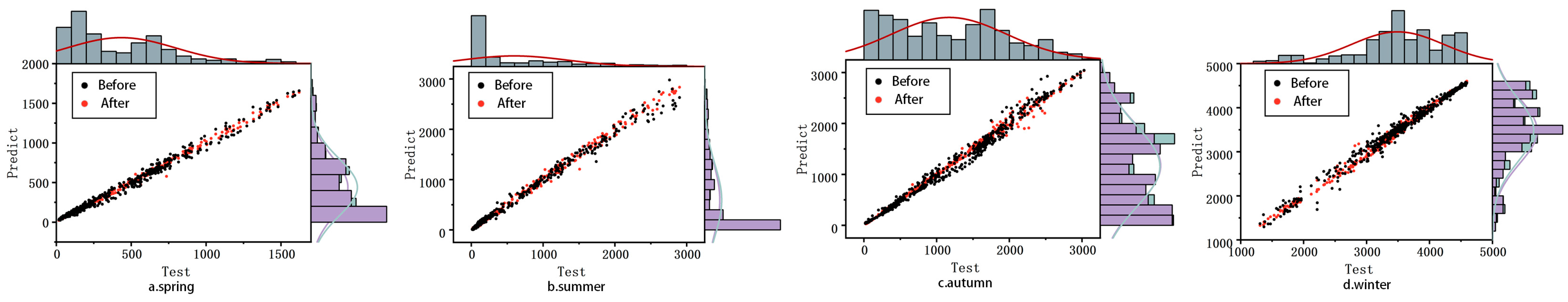
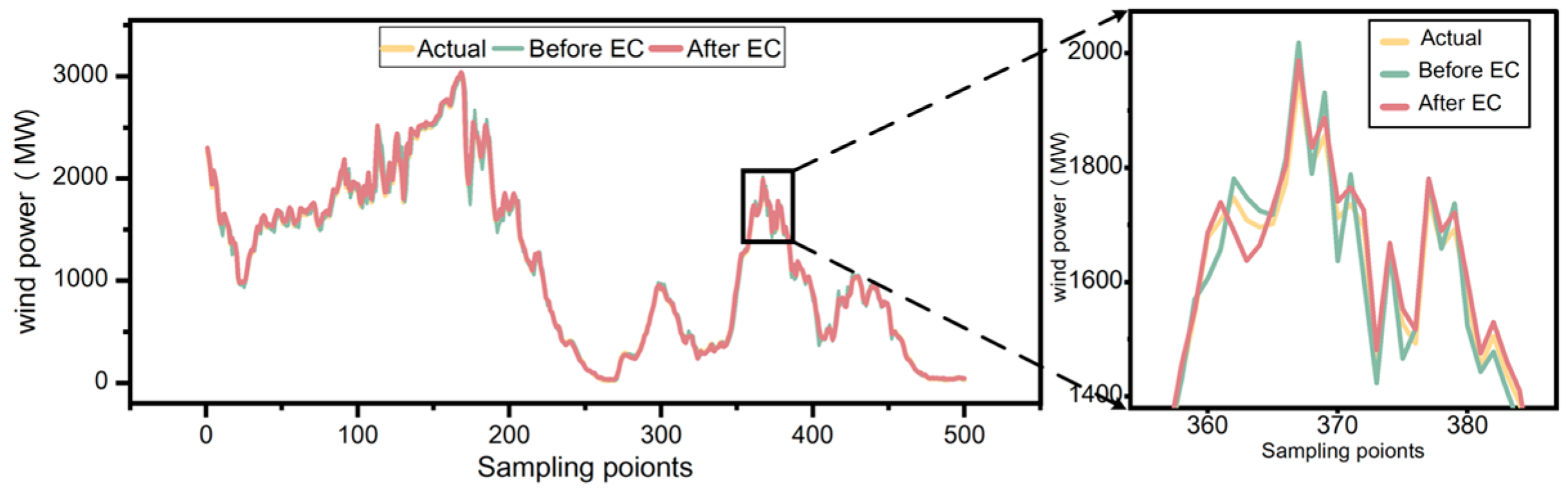
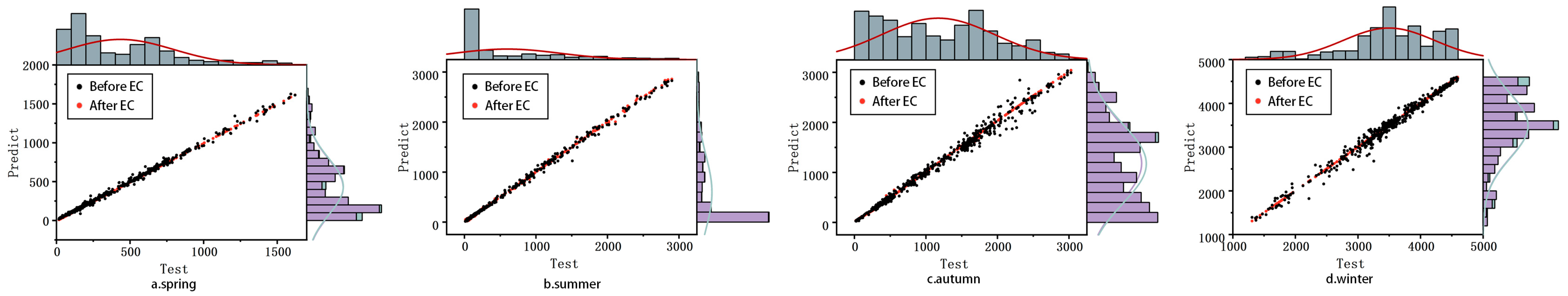
4.5. Analysis of Prediction Results of Error Correction Model

In order to verify the feasibility of the error correction model mentioned in Section 2.4, the integrated prediction model combined with error correction is used as the primary model for prediction analysis. To intuitively display the model’s prediction effect, the 1-step ahead prediction strategy is adopted in this subsection for error correction analysis. The following analysis presents the error distribution of the actual wind power value and predicted value for the wind farm before and after model error correction in all four seasons.

The error correction model was added to the forecast results in autumn, enabling a comparison between the forecast results before and after error correction, as shown in Figure 18. It can be concluded that, based on the recognition and segmentation of the power ramp in the integrated prediction model mentioned above, the predicted value is closer to the actual power during changes, and the overall prediction result more accurately reflects the actual wind power and follows the changing trend of the actual wind power. Specifically, the corrected forecast results not only better track the change path of real wind power in terms of overall trend, but also show smaller error fluctuations in numerical accuracy. Taking the typical slope periods in the figure as an example, the forecast results before error correction often show obvious lag or offset near the power mutation point, while the corrected curve can capture the position and amplitude of the power turning point more quickly.

Figure 19 presents the forecast distribution diagram of the wind power sequence for the wind farm in different seasons before and after error correction. The horizontal axis of the forecast value scatter distribution diagram after error correction represents the actual power value of the wind farm, while the vertical axis denotes the forecast value after wind power correction. The closer the points in the figure are to the line y = x, the better the model’s prediction effect. It can be clearly seen from the figure that after the error correction, the overall distribution of the forecast scatter points is more compact, most of the points are densely distributed near the direct proportional function, and the degree of deviation is significantly reduced. Compared with the “divergent” distribution of the forecast value before the error correction, the corrected results show a stronger linear correlation, indicating that the model has improved the forecast accuracy in multiple power intervals, and the forecast error has been effectively suppressed in different seasons.

The specific forecast error indicators are shown in Table 4: the MAE after correction in the four seasons is 6.8137, 12.2806, 31.7359, and 25.4016 lower than the uncorrected forecast results, respectively; MAPE is 0.0094, 0.0146, 0.0136, and 0.0015 lower than the uncorrected forecast results, respectively; RMSE is 13.5605, 19.2663, 57.2884, and 14.5087 lower than the uncorrected prediction results. Therefore, the proposed error prediction model can obtain relatively accurate prediction results and effectively reduce the prediction error. The error correction effect is more apparent when there are greater changes in wind power fluctuation frequency and amplitude.

5. Conclusions

This work aims to tackle the challenge of low prediction accuracy during rapid wind power fluctuations by proposing a graph neural network-based short-term forecasting method, which integrates ramp event recognition with real-time error correction. The approach begins with an improved ramp detection process, where wind power sequences are decomposed into three types based on ramp characteristics and their correlation with meteorological variables. On this basis, a multilayer GCN is applied to extract spatial and temporal features from the data, allowing ramp-type-aware prediction modeling. A real-time feedback mechanism is further introduced to dynamically correct forecast errors during operation.

Compared with conventional methods that do not differentiate between ramp phases, this model improves the segmentation of ramp events and builds a more expressive muti-event graph, which helps capture the influence of different meteorological factors. It also incorporates a closed-loop correction process that compensates for systematic deviations in the output.

Experimental results on the Elia dataset from a Belgian wind farm confirm that the proposed method significantly reduces prediction errors, especially during intense ramp events. Specifically, it achieves about a 28% improvement in prediction accuracy over baseline models and maintains high performance across various forecasting horizons. These findings indicate the method’s potential to enhance short-term wind power prediction in practical settings. Nonetheless, current limitations include the relatively simple meteorological feature set and the reliance on accurate prior ramp identification. Future improvements will focus on expanding the input feature space and refining the decomposition process to further enhance efficiency and reliability.

References

1. Farah, S.; David, W.A.; Humaira, N.; Aneela, Z.; Steffen, E. Short-term multi-hour ahead country-wide wind power prediction for Germany using gated recurrent unit deep learning. Renew. Sustain. Energy Rev. 2022, 167, 112700. [Google Scholar] [CrossRef]
2. Hanifi, S.; Liu, X.L.; Lin, Z.; Lotfian, S. A critical review of wind power forecasting methods-past, present and future. Energies 2020, 13, 3764. [Google Scholar] [CrossRef]
3. Cao, B.; Chang, L. Development of short-term wind power forecasting methods. In Proceedings of the 2022 IEEE 7th Southern Power Electronics Conference, SPEC, Nadi, Fiji, 5–8 December 2022. [Google Scholar]
4. Global Wind Report 2024—Global Wind Energy Council. Available online: https://www.gwec.net/reports/globalwindreport/2024 (accessed on 3 July 2024).
5. González-Sopeña, J.; Pakrashi, V.; Ghosh, B. An overview of performance evaluation metrics for short-term statistical wind power forecasting. Renew. Sustain. Energy Rev. 2021, 138, 110515. [Google Scholar] [CrossRef]
6. Wang, H.; Zhang, N.; Du, E.; Yan, J.; Han, S.; Liu, Y. A comprehensive review for wind, solar, and electrical load forecasting methods. Glob. Energy Interconnect. 2022, 5, 9–30. [Google Scholar] [CrossRef]
7. Liu, H.; Li, Y.; Duan, Z.; Chen, C. A review on multi-objective optimization framework in wind energy forecasting techniques and applications. Energy Convers. Manag. 2020, 224, 113324. [Google Scholar] [CrossRef]
8. He, J.J.; Yu, C.J.; Li, Y.L.; Xiang, H.Y. Ultra-short term wind prediction with wavelet transform, deep belief network and ensemble learning. Energy Convers. Manag. 2020, 205, 112418. [Google Scholar] [CrossRef]
9. Jiang, Y.; Chen, Y.C.; Kun, Y.U.; Liao, Y.C. Short-term wind power forecasting using hybrid method based on enhanced boosting algorithm. J. Mod. Power Syst. Clean Energy 2017, 5, 126–133. [Google Scholar] [CrossRef]
10. Lin, Z.; Liu, X.; Collu, M. Wind power prediction based on high-frequency SCADA data along with isolation forest and deep learning neural networks. Int. J. Electr. Power Energy Syst. 2020, 118, 105835. [Google Scholar] [CrossRef]
11. Lu, P.; Ye, L.; Zhao, Y.; Dai, B.; Pei, M.; Tang, Y. Review of meta-heuristic algorithms for wind power prediction: Methodologies, applications and challenges. Appl. Energy 2021, 301, 117446. [Google Scholar] [CrossRef]
12. Dhiman, H.S.; Deb, D.; Guerrero, J.M. On wavelet transform based convolutional neural network and twin support vector regression for wind power ramp event prediction. Sustain. Comput. Inform. Syst. 2022, 36, 100795. [Google Scholar] [CrossRef]
13. Zhou, B.; Duan, H.; Wu, Q.; Wang, H.; Or, S.W.; Chan, K.W.; Meng, Y. Short-term prediction of wind power and its ramp events based on semi-supervised generative adversarial network. Int. J. Electr. Power Energy Syst. 2021, 125, 106411. [Google Scholar] [CrossRef]
14. He, B.; Ye, L.; Pei, M.; Lu, P.; Dai, B.; Li, Z.; Wang, K. A combined model for short-term wind power forecasting based on the analysis of numerical weather prediction data. Energy Rep. 2022, 8, 929–939. [Google Scholar] [CrossRef]
15. Lu, P.; Ye, L.; Pei, M.; Zhao, Y.; Dai, B.; Li, Z. Short-term wind power forecasting based on meteorological feature extraction and optimization strategy. Renew. Energy 2022, 184, 642–661. [Google Scholar] [CrossRef]
16. Yang, T.; Yang, Z.; Li, F.; Wang, H. A short-term wind power forecasting method based on multivariate signal decomposition and variable selection. Appl. Energy 2024, 360, 122759. [Google Scholar] [CrossRef]
17. Hou, G.; Wang, J.; Fan, Y. Multistep short-term wind power forecasting model based on secondary decomposition, the kernel principal component analysis, an enhanced arithmetic optimization algorithm, and error correction. Energy 2023, 286, 129640. [Google Scholar] [CrossRef]
18. Yang, M.; Che, R.; Yu, X.; Su, X. Dual NWP wind speed correction based on trend fusion and fluctuation clustering and its application in short-term wind power prediction. Energy 2024, 302, 131802. [Google Scholar] [CrossRef]
19. Yang, M.; Wang, D.; Xu, C.; Dai, B.; Ma, M.; Su, X. Power transfer characteristics in fluctuation partition algorithm for wind speed and its application to wind power forecasting. Renew. Energy 2023, 211, 582–594. [Google Scholar] [CrossRef]
20. Yang, M.; Guo, Y.; Huang, Y. Wind power ultra-short-term prediction method based on NWP wind speed correction and double clustering division of transitional weather process. Energy 2023, 282, 128947. [Google Scholar] [CrossRef]
21. Ye, L.; Li, Y.; Pei, M.; Zhao, Y.; Li, Z.; Lu, P. A novel integrated method for short-term wind power forecasting based on fluctuation clustering and history matching. Appl. Energy 2022, 327, 120131. [Google Scholar] [CrossRef]
22. Yang, M.; Wang, T.; Zhang, X.; Zhang, W.; Wang, B. Considering dynamic perception of fluctuation trend for long-foresight-term wind power prediction. Energy 2023, 289, 130016. [Google Scholar] [CrossRef]
23. Zhao, B.; He, X.; Ran, S.; Zhang, Y.; Cheng, C. Spatial correlation learning based on graph neural network for medium-term wind power forecasting. Energy 2024, 296, 131164. [Google Scholar] [CrossRef]
24. Xiao, F.; Ping, X.; Li, Y.; Xu, Y.; Kang, Y.; Liu, D.; Zhang, N. The Short-Term Prediction of Wind Power Based on the Convolutional Graph Attention Deep Neural Network. Energy Eng. 2024, 121, 359–376. [Google Scholar] [CrossRef]
25. Lv, Y.; Hu, Q.; Xu, H.; Lin, H.; Wu, Y. An ultra-short-term wind power prediction method based on spatial-temporal attention graph convolutional model. Energy 2024, 293, 130751. [Google Scholar] [CrossRef]
26. Cui, Y.; Chen, Z.; He, Y.; Xiong, X.; Li, F. An algorithm for forecasting day-ahead wind power via novel long short-term memory and wind power ramp events. Energy 2022, 263, 125888. [Google Scholar] [CrossRef]
27. Tascikaraoglu, A.; Uzunoglu, M. A review of combined approaches for prediction of short-term wind speed and power. Renew. Sustain. Energy Rev. 2014, 34, 243–254. [Google Scholar] [CrossRef]
28. Wu, X.; Sun, R.; Qiao, Y.; Lu, Z. Estimation of error distribution for wind power prediction based on power curves of wind farms. Power Syst. Technol. 2017, 41, 1801–1807. [Google Scholar]
29. Zhao, J.; Guo, Y.; Xiao, X.; Wang, J.; Chi, D.; Guo, Z. Multi-step wind speed and power forecasts based on a WRF simulation and an optimized association method. Appl. Energy 2017, 197, 183–202. [Google Scholar] [CrossRef]
30. Wang, Q.; Yu, P.; Lv, M.; Wu, X.; Li, C.; Chang, X.; Wu, L. Real-time prediction of wave-induced hull girder loads for a large container ship based on the recurrent neural network model and error correction strategy. Int. J. Nav. Arch. Ocean Eng. 2024, 16, 100587. [Google Scholar] [CrossRef]
31. Zhang, S.; Liu, M.; Liu, M.; Lei, Z.; Zeng, G.; Chen, Z. Day-ahead wind power prediction using an ensemble model considering multiple indicators combined with error correction. Appl. Soft Comput. 2023, 148, 110873. [Google Scholar] [CrossRef]
32. Ye, L.; Dai, B.; Li, Z.; Pei, M.; Zhao, Y.; Lu, P. An ensemble method for short-term wind power prediction considering error correction strategy. Appl. Energy 2022, 322, 119475. [Google Scholar] [CrossRef]
33. Hu, J.; Zhang, L.; Tang, J.; Liu, Z. A novel transformer ordinal regression network with label diversity for wind power ramp events forecasting. Energy 2023, 280, 128075. [Google Scholar] [CrossRef]
34. Dalton, A.; Bekker, B.; Koivisto, M.J. Simulation and detection of wind power ramps and identification of their causative atmospheric circulation patterns. Electr. Power Syst. Res. 2021, 192, 106936. [Google Scholar] [CrossRef]
35. Gallego-Castillo, C.; Cuerva-Tejero, A.; Lopez-Garcia, O. A review on the recent history of wind power ramp forecasting. Renew. Sustain. Energy Rev. 2015, 52, 1148–1157. [Google Scholar] [CrossRef]
36. Zhang, J.; Cui, M.; Hodge, B.-M.; Florita, A.; Freedman, J. Ramp forecasting performance from improved short-term wind power forecasting over multiple spatial and temporal scales. Energy 2017, 122, 528–541. [Google Scholar] [CrossRef]
37. Zhao, Y.; Liao, H.; Pan, S.; Zhao, Y. Interpretable multi-graph convolution network integrating spatio-temporal attention and dynamic combination for wind power forecasting. Expert Syst. Appl. 2024, 255, 124766. [Google Scholar] [CrossRef]
38. Wei, C.; Pi, D.; Ping, M.; Zhang, H. Short-term load forecasting using spatial-temporal embedding graph neural network. Electr. Power Syst. Res. 2023, 225, 109873. [Google Scholar] [CrossRef]
39. Zhao, J.; Yan, Z.; Zhou, Z.; Chen, X.; Wu, B.; Wang, S. A ship trajectory prediction method based on GAT and LSTM. Ocean Eng. 2023, 289, 116159. [Google Scholar] [CrossRef]
40. Wei, Y.; Chen, Z.; Zhao, C.; Chen, X.; He, J.; Zhang, C. A three-stage multi-objective heterogeneous integrated model with decomposition-reconstruction mechanism and adaptive segmentation error correction method for ship motion multi-step prediction. Adv. Eng. Inform. 2023, 56, 101954. [Google Scholar] [CrossRef]
Figure 1. Representational quantity of ramp events.
Energies 18 02763 g001
Figure 2. Multi-layer GCN structure. (A) Input layer; (B) Output layer.
Energies 18 02763 g002
Figure 3. GCN model architecture.
Energies 18 02763 g003
Figure 4. Error correction flowchart.
Energies 18 02763 g004
Figure 5. Framework of the integrated wind power prediction. The red star here represents the location of the wind farm.
Energies 18 02763 g005
Figure 6. Wind power generation of a wind farm in Belgium in 2022.
Energies 18 02763 g006
Figure 7. Schematic diagram of four seasons wind power ramp classification.
Energies 18 02763 g007
Figure 8. Correlation heat map analysis.
Energies 18 02763 g008
Figure 9. Adjacency matrix of different climbing events. The darker the color, the stronger the correlation, and the lighter the color, the weaker the correlation.
Energies 18 02763 g009
Figure 10. Relationship diagram between different thresholds and errors.
Energies 18 02763 g010
Figure 11. The prediction results before and after the recognition of ramp features.
Energies 18 02763 g011aEnergies 18 02763 g011b
Figure 12. Prediction results of four seasons of several forecasting models 1-step ahead.
Energies 18 02763 g012
Figure 13. Prediction results of the four seasons of several forecasting models 2-step ahead.
Energies 18 02763 g013
Figure 14. Prediction results of the four seasons of several forecasting models 3-step ahead.
Energies 18 02763 g014
Figure 15. Considers the four-season prediction error distribution before and after ramp recognition.
Energies 18 02763 g015
Figure 16. Prediction results of multi-step ahead of the four seasons of several forecasting models.
Energies 18 02763 g016
Figure 17. One-step prediction error distribution of different forecasting models in different seasons.
Energies 18 02763 g017
Figure 18. Prediction results before and after error correction (Autumn).
Energies 18 02763 g018
Figure 19. Prediction error distribution before and after error correction of wind farm four-season model.
Energies 18 02763 g019