Performance Analysis of Artificial Intelligence Models for Classification of Transmission Line Losses

Abstract

Conventional approaches to analyzing power losses in electrical transmission networks have largely emphasized generic power loss minimization through the integration of loss-reducing devices such as shunt capacitors. However, achieving optimal power loss minimization requires a more data-driven and intelligent approach that transcends traditional methods. This study presents a novel classification-based methodology for detecting and analyzing transmission line losses using real-world data from the Ikorodu–Sagamu 132 kV double-circuit line in Nigeria, selected for its dense concentration of high-voltage consumers. Twelve (12) transmission lines were examined, and the collected data were subjected to comprehensive preprocessing, feature engineering, and modeling. The classification capabilities of advanced deep learning models—Long Short-Term Memory (LSTM), Bidirectional Long Short-Term Memory (BiLSTM), and Gated Recurrent Unit (GRU)—were explored through six experimental scenarios: LSTM, LSTM with Attention Mechanism (LSTM-AM), BiLSTM, GRU, LSTM-BiLSTM, and LSTM-GRU. These models were implemented using the Python programming environment and evaluated using standard performance metrics, including accuracy, precision, recall, F1-score, support, and confusion matrices. Statistical analysis revealed significant variability in transmission losses, particularly in lines such as I1, Ps, Ogy, and ED, which exhibited high standard deviations. The LSTM-AM model achieved the highest classification accuracy of 83.84%, outperforming both standalone and hybrid models. In contrast, BiLSTM yielded the lowest performance. The findings demonstrate that while standalone models like GRU and LSTM are effective, the incorporation of attention mechanisms into LSTM architecture enhances classification accuracy. This study provides a compelling case for employing deep learning-based classification techniques in intelligent power loss classification across transmission networks. It also supports the realization of SDG 7 by aiming to provide access to reliable, affordable, and sustainable energy for all.

1. Introduction

Energy is an essential commodity required for the seamless operation of industrial processes, as well as commercial and residential activities. It plays a pivotal role in powering homes, organizations, and industries [1,2,3]. This energy can be derived from either conventional fossil fuels or renewable resources. Regardless of the source, the energy delivery chain typically consists of three primary stages: generation (the production hub), transmission (the bulk conveyance of energy), and distribution (ensuring that end users receive quality power for consumption) [4,5,6]. In simpler terms, electrical energy is generated, transmitted over long distances, and ultimately distributed to consumers through a network infrastructure. While the distribution network is often more complex due to its structure and the variability of voltage requirements among consumers, the transmission network is comparatively simpler due to the absence of direct load connections [7,8,9,10]. Transmission lines consist of several essential components—conductors, insulators, shield wires, and support structures—each contributing to the system’s overall performance. Among these, conductors are especially important, as inadequate design can result in substantial and costly energy losses during transmission [11,12].

Energy losses, commonly referred to as “losses”, are a frequent and often unavoidable occurrence in both transmission and distribution networks. These electrical losses represent the gap between the energy generated and the amount that end users are billed for, essentially reflecting unaccounted-for energy [13,14]. Transmission and distribution (T\&D) losses have been reported to account for approximately 30% of the hidden costs in Africa’s energy sector [15].

Electrical network losses are typically categorized into two types: technical losses (TL) and non-technical losses (NTL). NTLs are caused by factors such as energy theft, meter tampering, faulty or bypassed meters, unmetered supply, and inaccurate meter readings. [13,16,17,18]. At the grid level, these losses can result in transformer overload, voltage imbalance, and uncertainty in consumption data. Importantly, non-technical losses (NTLs) negatively impact honest consumers by driving up electricity prices and degrading energy quality. An increase in NTLs often leads to higher energy tariffs and diminished system reliability [19]. Numerous studies have focused on identifying the root causes of non-technical losses (NTLs) and developing effective mitigation strategies [13,20]. Detecting NTLs is a crucial step in addressing them. One study [21] examined non-hardware-based NTL detection techniques, categorizing them into hardware-based and non-hardware-based approaches. The study highlighted that hardware-based methods often require substantial capital investment and increase energy costs due to the need for new infrastructure. In contrast, non-hardware-based methods use system and consumer data to identify abnormal usage patterns, which were further divided into network-based, data-based, and hybrid techniques. Notably, a study [22] employed a data-based approach for theft detection, utilizing consumption data from smart meters and clustering methods. They applied a distance-based classification technique to identify anomalies using the Gustafson–Kessel fuzzy clustering algorithm. Their model evaluated sixteen scenarios representing abnormal consumption patterns caused by NTLs, achieving a true positive rate of 63.6% and a false positive rate of 24.3%, outperforming other unsupervised learning techniques.

Artificial intelligence (AI)-based approaches for NTL detection have proven to be more accurate, efficient, and faster than traditional methods [23]. These studies provide comprehensive reviews of AI-driven NTL detection techniques, classifying them based on algorithms, extracted features, and performance metrics. Comparative evaluations of data-based, network-based, and hybrid methods offer valuable insights for both researchers and industry practitioners. In contrast, technical losses (TLs) have received less research attention due to the complexity and challenges involved in detection [24]. TLs result from inherent electrical properties, such as network impedance. For example, [25] analyzed data from a distribution company to estimate losses and billing efficiency on 11kV feeders, linking distribution losses to factors like meter bypassing, tampering, incorrect billing, illegal connections, non-payment, and aging infrastructure. Another study [26] focused on reducing transmission losses in wind-integrated networks using mixed-integer nonlinear programming (MINLP).

Artificial intelligence (AI) is playing an increasingly vital role in modern energy systems. Smart grids, equipped with intelligent devices and sensors, are designed to improve the distribution, control, and generation of electricity. For instance, machine learning-based smart meters are essential in Ambient Assistive Living (AAL) environments, where they help identify consumption patterns [27]. AI is often integrated with edge computing and analytics to enhance system modeling and responsiveness. The effectiveness of smart grids, smart homes, and smart meters relies heavily on the integration of AI with secure communication technologies. Common AI techniques used in smart grids include machine learning, deep learning, and swarm intelligence, all of which are crucial for data analytics, system security, and automation in Internet of Things (IoT)-enabled environments [28,29,30]. The progression to “AI 2.0” has been driven by advancements in both algorithms and computing hardware. Technologies such as deep learning and reinforcement learning have matured, and their combination—deep reinforcement learning (DRL)—has reached significant milestones, notably demonstrated by AlphaGo’s victory over Go champion Sedol Lee [31].

The power systems sector has seen significant advancements through the adoption of artificial intelligence (AI), particularly in the detection and reduction of losses. Velasco et al. [32] demonstrated that deep learning models offer faster convergence for estimating technical losses, enabling near real-time operations. Coma-Puig et al. [33] investigated the application of explainable AI (XAI) for detecting non-technical losses (NTLs) in electricity and gas networks, resulting in notable improvements in system performance. Almasoudi [34] concluded that AI integration enhances the resilience, efficiency, and sustainability of power systems. His work employed hybrid convolutional neural network (CNN) architectures—such as CNN-RNN, CNN-GRU, and CNN-LSTM—for effective fault detection and analysis.

Shafei et al. [35] applied a CNN-based approach to fault detection and characterization in medium-voltage distribution networks. In the field of civil engineering, CNN-based structural damage detection under limited data conditions was performed using transfer learning techniques [36]. Similarly, [37] developed an intelligent method for detecting defects in electricity transmission line equipment, using data mining and improving performance through CNN-based models enhanced with transfer learning. In another study, [38] proposed a novel hybrid approach for fault detection and identification in transmission lines within interconnected networks, utilizing data from phasor measurement units (PMUs).

The reviewed literature makes it clear that while numerous detection systems exist, many fall short in their ability to support informed, technical decision-making for effective loss mitigation. Most systems are designed to identify losses but fail to classify the loss type, thereby hindering actionable insights that network operators can use to implement timely and strategic interventions. This gap is particularly critical in the context of Africa’s ongoing energy crisis, where energy losses—especially in transmission networks—pose a severe challenge. Given that transmission lines carry large volumes of electricity, even minor losses can cascade into substantial shortages at the distribution level. Minimizing these losses is, therefore, not just a technical necessity but a strategic imperative for achieving energy sufficiency across the continent.

To address this pressing issue, the development of a next-generation energy loss management system is essential—one that goes beyond mere detection. Such a system must be capable of identifying the root causes of losses in real-time and recommending effective remedial actions. A key insight from the literature is that one of the main obstacles to effective loss mitigation is the accurate classification of loss types. Without this, interventions remain generic and suboptimal. While many existing approaches focus on reducing power losses through conventional means, such as the strategic placement of equipment like shunt capacitors, these solutions often overlook the need for intelligent, context-specific strategies.

This study responds to that need by applying advanced AI techniques to classify transmission losses with high precision. By doing so, it lays the groundwork for smarter, more targeted network management—equipping utility providers with the tools they need to make data-driven decisions, enhance grid reliability, and move closer to sustainable energy goals.

The main contributions of the present study are as follows:

(1)

This study introduces a novel classification-based methodology using deep learning models (LSTM, GRU, BiLSTM, and hybrids) to detect and analyze transmission line losses based on real-world high-voltage network data from Nigeria, moving beyond conventional loss minimization techniques.

(2)

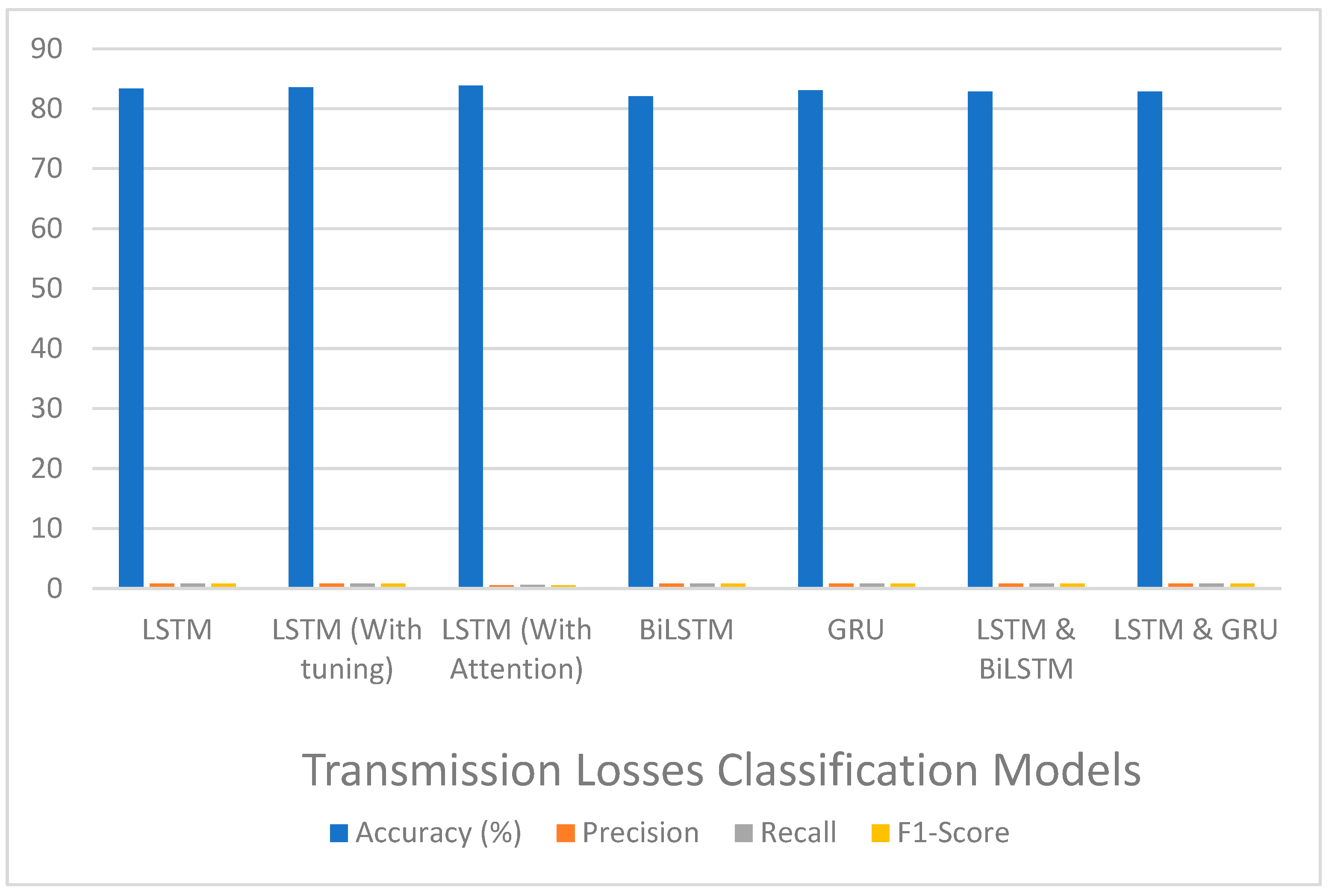
It is among the first to apply a comparative deep learning framework—including attention mechanisms (LSTM-AM)—for loss classification across multiple scenarios, with LSTM-AM achieving the highest accuracy of 83.84%.

(3)

The research highlights the significance of data preprocessing, feature engineering, and statistical variability analysis as diagnostic tools for identifying loss-prone lines and informing targeted interventions.

(4)

By providing actionable insights for intelligent transmission loss management, the study contributes to the advancement of data-driven energy systems aligned with the goals of affordable and reliable electricity access.

2. Materials and Method

This study investigates the classification of transmission losses as a strategic approach to improving loss management within electrical transmission networks. The predictive capabilities of AI models were leveraged to classify power losses using historical transmission line data. The architectures of the implemented AI models were developed and simulated within a Python-based environment. Model performance was rigorously evaluated using standard classification metrics, including accuracy, precision, recall, F1-score, support, and confusion matrices.

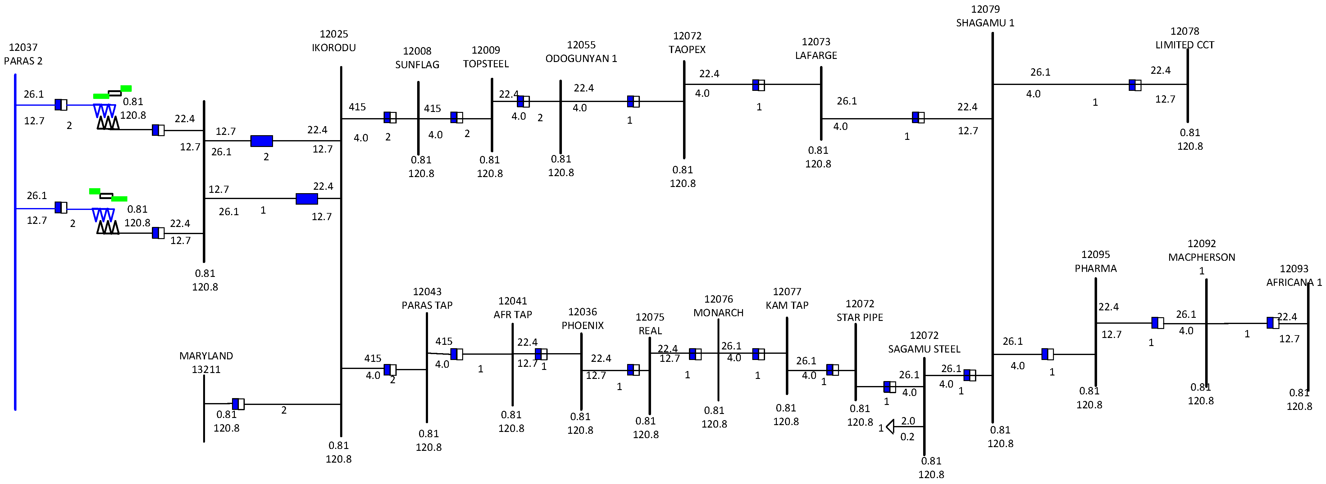
2.1. Transmission Line Data Collection and Preprocessing

The dataset utilized in this study was collected using a Schneider PM5100 smart energy meter from the Ikorodu–Sagamu 132 kV double-circuit transmission line shown in Figure 1, which serves as the selected case study. This particular line holds strategic significance within the Nigerian power grid due to the high concentration of industrial high-voltage consumers connected at the 132 kV level. Notable among these consumers are Sunflag, Monarch, and African Foundry, all of which are linked via Tee-offs along the line—transforming the transmission route into a complex, network-like structure. The primary power supply to this corridor originates from the Egbin Steam Power Plant through the Egbin–Ikorodu double-circuit line, while an auxiliary supply is provided by the Ayede–McPherson–Sagamu 132 kV line. Owing to the substantial load demand in the region, the Sagamu and Ijebu Ode 132/33 kV substations are supplied from Ayede, whereas the remaining load centers are primarily fed by the Egbin–Ikorodu line.

During data collection, inconsistencies emerged, as certain feeders were not consistently represented across all monthly records. To ensure a robust and uniform analysis, twelve (12) feeders out of the fifteen (15) detailed in

Table 1. List of T-offs in Ikorodu–Sagamu 132kV Double Circuit Line.

S/N	Lines	Line Code	Circuit
1	Ikorodu	12,025	1
2	Sunflag	12,008	1
3	Topsteel	12,009	1
4	Odogunyan 1	12,055	1
5	Taopex	12,072	1
6	Lafarge	12,073	1
7	Paras_1	12,037	2
8	Paras Tap1	12,043	2
9	AFR Tap	12,041	2
10	Phoenix	12,036	2
11	Real	12,075	2
12	Monarch	12,076	2
13	Kam Tap	12,077	2
14	Star Pipe	12,078	2
15	Sagamu Steel	12,079	2

from the Ikorodu–Sagamu 132 kV double-circuit line were systematically selected for model development. The dataset was organized into two time series: one for actual power values and another for forecasted power. These series were subjected to preprocessing and feature engineering, followed by a chronological train-test split. For model development, the Long Short-Term Memory (LSTM), Bidirectional LSTM (BiLSTM), and Gated Recurrent Unit (GRU) models were employed, necessitating the sequencing of data with a time step of one. Finally, both input and output datasets for training and testing were reshaped to meet the models’ input requirements. A sample of the preprocessed dataset is presented in

Table 2. Loss data head for the case study.

AFL	I1	I 2	Ks	Ps	Phx	Qt	Sp	Sf	Tp	Ts	Ogy	TG	TL	Bl	ED
4.07	13.58	102.41	0.000	18.06	8.99	3.42	2.35	1.76	11.16	0.94	21.2	29.22	21.530	0.330	123.68
3.75	17.41	97.56	0.000	0.00	8.95	3.16	1.94	1.56	10.13	0.75	20.7	10.13	20.110	−0.590	104.99
3.66	21.43	97.72	2.344	0.00	10.03	1.88	2.33	1.60	11.32	0.77	20.2	11.32	22.614	2.414	107.85
4.40	5.35	87.78	2.348	0.00	11.38	1.93	1.92	1.07	11.32	0.60	21.2	11.32	23.648	2.448	80.80
4.33	1.75	97.40	2.351	0.00	10.57	2.28	2.08	1.27	11.32	0.64	23.7	11.32	23.521	−0.178	86.94

AFL = African foundaries limited, I1 = Ikorodu1, I2 = Ikorodu2, Ks = Kamsteel, Ps = Paras, Phx = Phoenix, Qt = Quantum, Sp = Starpipe, Sf = Sunflag, Tp = Taopex, Ts = Topsteel, Ogy = Odogunyan, TG = Total Generation, TL = Total Loss, Bl = Bilateral, ED = Energy Difference.

. The loss threshold values for the loss types were presented as a percentage of the energy difference (ED) on the network under consideration. For the case study, the relationship between ED, total load (TL), and total generation (TG) is expressed in Equations (1)–(3).

$$TL=Ogy-Bl$$

(1)

$$TG=Tp-Ps$$

(2)

$$ED=TG+I1+I2-TL$$

(3)

where $TL$ is the total load, $Ogy$ is the Odogunyan line, $Bl$ represents all other bilaterals, $TG$ represents the total generation, $Tp$ represents the Taopex line, $Ps$ represents the Paras line, $ED$ represents the Energy Difference, $I1$ represents Ikorodu line 1, and $I2$ represents Ikorodu line 2. The $ED$, which represents the Energy Difference between the sending end and the receiving end, is an industry standard used to identify the losses recorded within a system, according to

Table 3. Loss threshold values.

Category	Description
Energy Theft	40% and above Energy Difference
Resistive Loss	30% and 40% Energy Difference
Corona Loss	20% to 30% Energy Difference
Reactive Loss	10% and 20% Energy Difference
Normal Loss	5% to 10% Energy Difference
Metering Issues	Less than 5% Energy Difference

, where six types of losses are categorized.

The steps used for the preprocessing and feature engineering pipeline are discussed subsequently:

• Identify columns with null values:

FOR each column IN dataset: IF count_missing_values(column) > 0: flag column

2.

Datetime Formatting: the date strings were converted to datetime objects:

FOR each entry IN ‘date’: convert to datetime format (dd/mm/yyyy hh:mm)

3.

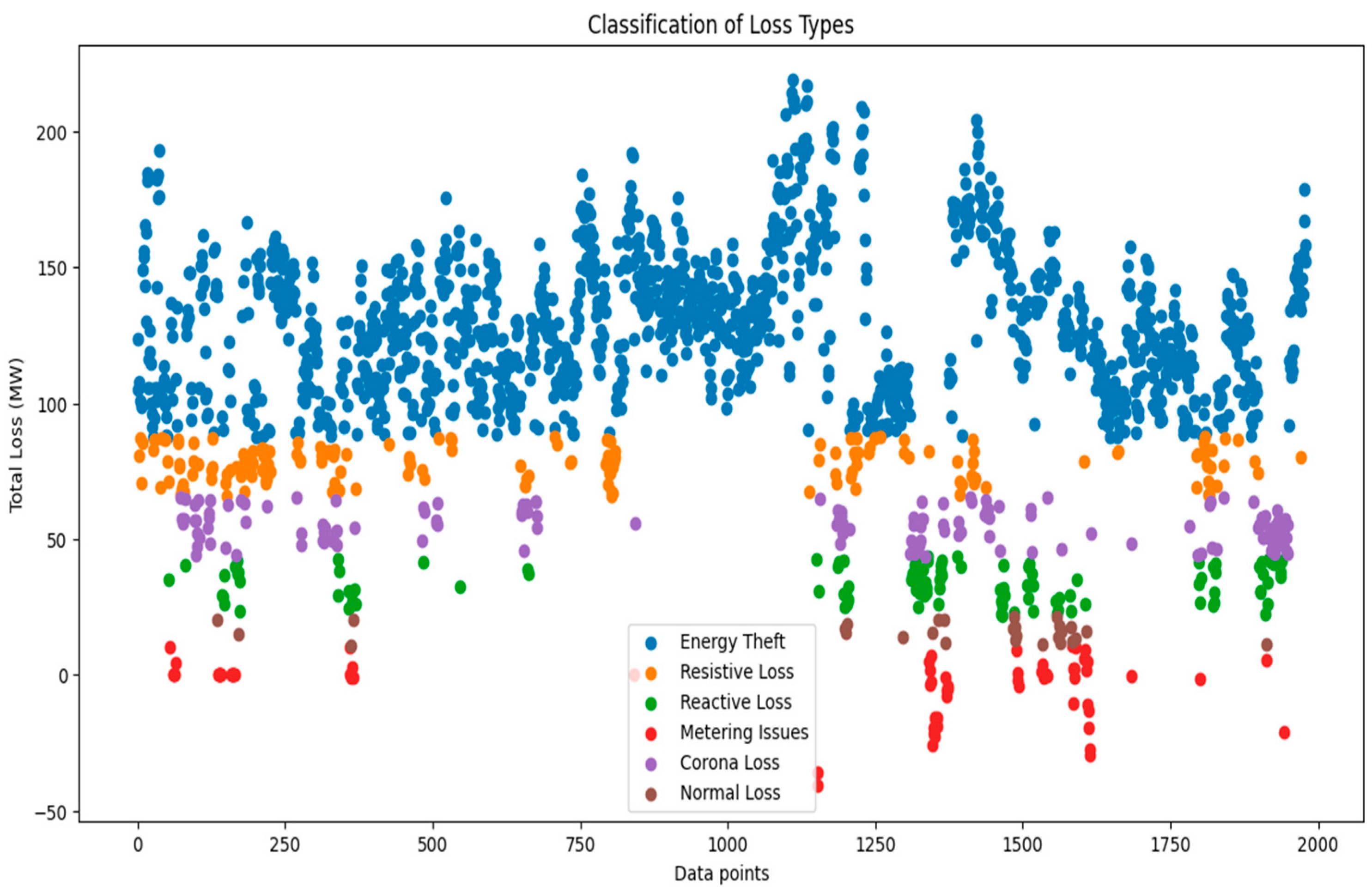
Engineering of loss type classes: used the ‘Energy Difference’ column values to categorize the loss types into classes using the threshold values in Table 3.

4.

Label Encoding: The categorical ‘loss_type’ labels were transformed into a numerical format using ‘label encoding’ to ensure compatibility with the neural network models. This was performed via this pseudocode:

Assign a unique integer to each distinct value in the ‘loss_type’ column.

5.

Select all the 12 loss lines and drop less important features, such as datetime, ED, TG, TL, and BI, as shown in Table 2.

6.

Feature Normalization: all numeric features were normalized to the [0, 1] range using the Min-max feature scaling, as seen in the equation below:

$$x_{scaled}={\displaystyle \frac{x-x_{min}}{x_{max}-x_{min}}}$$

7.

Time-series sequencing: for temporal models like LSTM, GRU, and BiLSTM, the data was reshaped into sequences using a sliding window approach:

FOR i = 0 TO N—time_steps:

X[i] = X[i:i + time_steps],

y[i] = y[i + time_steps]

where N = Number of samples

Each sequence consisted of a defined number of previous time steps (time_steps), and the corresponding target was the value at the next time step.

A time step of 1 was sufficient for this use case, as the dataset represented shorter dependencies. Although multiple time steps were tested, it did not improve the model accuracy.

8.

Train-test splitting: shuffle data randomly and allocate 80% for training and 20% for testing.

2.2. Transmission Line Losses Modeling

The notion behind power loss is based on the deviation of the voltage and current between the sending end and the receiving end. In Figure 2, consider that the transmission line length is Δx with resistance RΔx, conductance GΔ, current $I$, and voltage $V$. By applying Kirchhoff’s voltage law to this circuit, it can be written that

$$V={\displaystyle \frac{1}{2}}RI∆x+{\displaystyle \frac{1}{2}}R\left[I+∆I\right]∆x+V+∆V$$

(4)

By simplifying the equation by dividing through by $∆x$ and tending it to zero, Equation (4) becomes

$${\displaystyle \frac{dV}{dx}}=-RI$$

(5)

Taking the second derivative of Equation (5) yields Equation (6) as follows:

$${\displaystyle \frac{d^{2}V}{d{x}^2}}=-R{\displaystyle \frac{dI}{dx}}$$

(6)

Again, the application of Kirchhoff’s current law to the transmission line equivalent circuit results in the current Equation (7).

$$I={\displaystyle \frac{1}{2}}G\left(V+{\displaystyle \frac{∆V}{2}}\right)∆x+C{\displaystyle \frac{d}{dt}}\left(V+{\displaystyle \frac{∆V}{2}}\right)∆x+I+∆I$$

(7)

where $C$ is the capacitance. Again, by simplifying the equation through dividing by $∆x$ and letting it tend to zero, Equation (7) becomes

$${\displaystyle \frac{dI}{dx}}=-\left[GV+C{\displaystyle \frac{dV}{dt}}\right]$$

(8)

Equation (8) can be further simplified by taking the limit ${\displaystyle \frac{dV}{dt}}$ to zero.

$${\displaystyle \frac{dI}{dx}}=-GV$$

(9)

Taking the second derivative of Equation (6) yields Equation (10) as follows:

$${\displaystyle \frac{d^{2}I}{d{x}^2}}=-G{\displaystyle \frac{dV}{dx}}$$

(10)

The substitution of Equations (5) and (9) into Equations (6) and (10), respectively, results in Equations (11) and (12) that characterize the power flow along the transmission lines.

$${\displaystyle \frac{d^{2}V}{d{x}^2}}=RGV$$

(11)

$${\displaystyle \frac{d^{2}I}{d{x}^2}}=RGI$$

(12)

Applying boundary conditions in Equations (13) and (14) to Equation (8) results in Equation (15), which represents voltage power flow as follows:

$$V\left(0\right)=V_0$$

(13)

$$V\left(l\right)=0, l\to \infty$$

(14)

$$V\left(x\right)=V_0{e}^{-x\sqrt{RG}}$$

(15)

Applying boundary conditions in Equations (16) and (17) to Equation (12) yields Equation (18), which represents the current power flow as follows:

$$I\left(0\right)=I_0$$

(16)

$$I\left(l\right)=0, l\to \infty$$

(17)

$$I\left(x\right)=I_0{e}^{-x\sqrt{RG}}$$

(18)

Here, $I_0$ and $V_0$ represent the initial current and voltage, respectively. Equations (15) and (18) enable the prediction of current and voltage at any point along a transmission line. It should be recalled that the resistance of the conductor and weather conditions are mainly responsible for the power loss along a transmission line; hence, it can be asserted that losses along a transmission line have two basic components, namely, ohmic $L_o$ and corona $L_c$ losses. Therefore, the total losses ($L_T$) along a transmission line can be modeled as

$$L_T=L_o+L_c$$

(19)

These components can be individually modeled as

$$L_o=I^{2}R$$

(20)

$$L_c=242{\displaystyle \frac{\left(f+25\right)}{\delta }}.\sqrt[4]{{\displaystyle \frac{r}{d}}}{\left(V-V_c\right)}^2.{\left(10\right)}^{-5}kW$$

(21)

Here, f is the frequency of transmission, δ is the air density factor, r is the conductor radius, d is the transmission lines spacing, representing the operating voltage, and Vc is the disruptive voltage. Substituting Equations (20) and (21) in Equation (19) yields Equation (22), expressed as follows

$$L_T={RI}^2+242{\displaystyle \frac{\left(f+25\right)}{\delta }}.\sqrt[4]{{\displaystyle \frac{r}{d}}}{\left(V-V_c\right)}^2.{\left(10\right)}^{-5}kW$$

(22)

Equation (22) can be used to evaluate the losses along a transmission line.

2.3. Models for Transmission Losses Management System

This section addresses the design of classification models of transmission losses using different classification models as presented as follows.

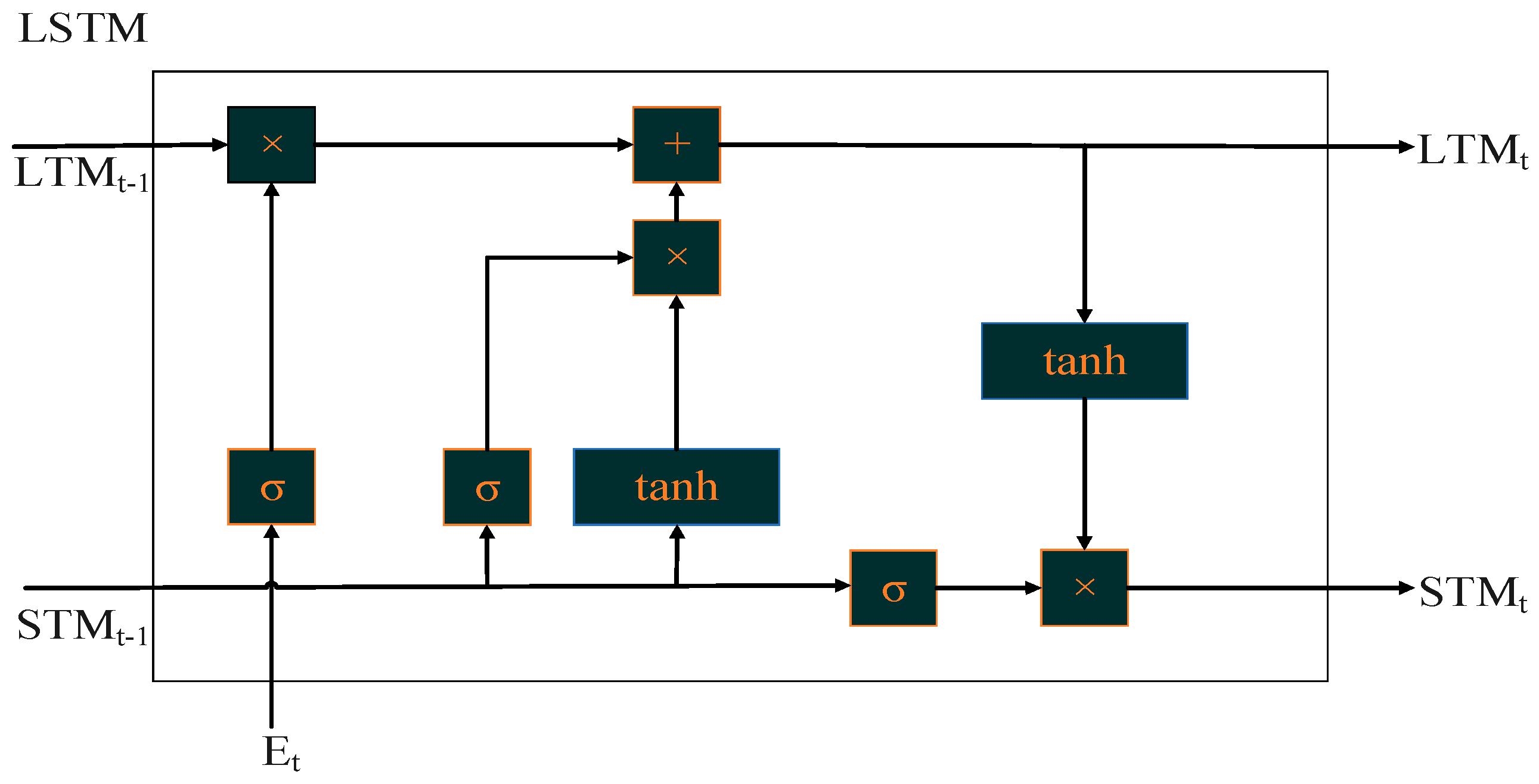
2.3.1. Long Short-Term Memory (LSTM) Model

The Long Short-Term Memory (LSTM) model, a specialized type of Recurrent Neural Network (RNN), is designed to effectively capture temporal dependencies and learn complex patterns in sequential data. In this study, the LSTM model was employed to classify transmission loss data due to its robust capability in handling time series inputs. LSTM networks are characterized by their use of memory cells and gating mechanisms, which enable them to retain, discard, or update information over time. As illustrated in Figure 3, the LSTM architecture comprises three primary gates: the input gate, the forget gate, and the output gate. These gates regulate the flow of information into and out of the memory cells, ensuring that only relevant data are propagated through the network. The input and forget gates determine how much new information is added and how much previous information is discarded from the cell state. The final output is a selectively filtered version of the internal cell state, influenced by the context of both current and past inputs. The behavior of the gates and the cell states can be mathematically described using the following Equations (23)–(28), based on the input time series $X_t$ and the number of hidden units $h$ [39]:

$$\mathrm{Input} \mathrm{Gate}: I_t=\sigma (X_t{W}_{xi}+H_{t-1}{W}_{hi}+b_i)$$

(23)

$$\mathrm{Forget} \mathrm{Gate}: F_t=\sigma (X_t{W}_{xf}+H_{t-1}{W}_{hf}+b_f)$$

(24)

$$\mathrm{Output} \mathrm{Gate}: O_t=\sigma (X_t{W}_{xo}+H_{t-1}{W}_{ho}+b_o)$$

(25)

$$\mathrm{Intermediate} \mathrm{Cell} \mathrm{State}: {\tilde{C}}_t=\tanh (X_t{W}_{xo}+H_{t-1}{W}_{ho}+b_c)$$

(26)

$$\mathrm{Cell} \mathrm{State} (\mathrm{next} \mathrm{memory} \mathrm{input}): C_t=F_t ° C_{t-1}{\tilde{C}}_t$$

(27)

$$\mathrm{New} \mathrm{State}: H_t=O_t ° \mathrm{t}\mathrm{a}\mathrm{n}\mathrm{h}\left(C_t\right)$$

(28)

Here, $W_{hi}, W_{xc}{,W}_{xf}, W_{xo}, and W_{hc},W_{hf},W_{ho }$ are the weight parameters, while $b_i, b_f,{b_c,b}_o$ symbolize bias parameters, $°$ represents the element-wise multiplication. Note that the estimation of $C_t$ depends on the output information from memory cells ($C_{t-1})$ and the current time step ${\tilde{C}}_t$.

2.3.2. Bidirectional Long Short-Term Memory (BiLSTM) Model

The Bidirectional Long Short-Term Memory (BiLSTM) network is an extension of the standard LSTM architecture that incorporates two parallel processing layers—one operating in the forward direction and the other in the backward direction. This dual-track structure enables the model to capture both past and future dependencies within a time series, thereby improving its temporal learning capability. As illustrated in Figure 4, the forward layer (indicated by the red arrow) processes the input sequence $X_t$ from left to right, while the backward layer (shown by the blue arrow) processes the same sequence in reverse, from right to left. The final output is obtained by combining the outputs from both directions, typically through a weighted sum or concatenation of the prediction scores. In this study, the BiLSTM architecture was employed to enhance classification performance by leveraging contextual information from both preceding and succeeding time steps.

2.3.3. Gated Recurrent Unit (GRU) Model

The Gated Recurrent Unit (GRU) model, a streamlined variant of the Long Short-Term Memory (LSTM) network, was employed in this study for the classification of transmission losses. Unlike LSTM, the GRU architecture utilizes a single hidden state and merges the functionalities of the input and forget gates into a single update gate. Additionally, it features a reset gate, which regulates the influence of the previous hidden state on the current hidden state, as depicted in Figure 5. Due to the absence of a separate cell state and the reduction in the number of gating mechanisms, GRUs require fewer parameters and involve fewer tensor operations. This simplification contributes to a faster training process and more efficient convergence. The mathematical formulation of the GRU cell is presented in Equations (29)–(32) [40]:

$$r_t=\sigma \left(W_{xr}{x}_{\left[t\right]}+b_{xr}+W_{hr}{h}_{\left[t-1\right]}+b_{hr}\right)$$

(29)

$$z_t=\sigma \left(W_{xz}{x}_{\left[t\right]}+b_{xz}+W_{hz}{h}_{\left[t-1\right]}+b_{hz}\right)$$

(30)

$$k_t=tanh\left(W_{xk}{x}_{\left[t\right]}+b_{xk}+r_t{\odot (W}_{hk}{h}_{\left[t-1\right]}+b_{hk})\right)$$

(31)

$$h_{\left[t\right]}=\left(1-z_t\right)\odot k_t+z_t\odot h_{\left[t-1\right]}$$

(32)

Here, $\sigma$, $tanh$, and $\odot$ are used as the elements of the weight matrices $W_x$, $W_h$, $b_x$, and $b_h$.

2.3.4. Input–Output Design of the Models

The input–output design of the models used in this study is outlined as follows:

• Input Structure

The input data consists of sequences of time-series observations. Each sequence is made up of time_steps past observations, where each time step contains multiple features such as African Foundries Limited, Kamsteel, Sunflag, and other energy-related variables (12 features in total as shown in Table 2). A sliding window approach was used to generate these sequences. Each input sequence represents the data from the previous time_steps and is fed into the model as input for predicting the loss type at the subsequent time step.

2.

Output Structure

The model’s task is to classify the loss type (e.g., “Energy Theft”, “Resistive Loss”, etc.) based on the input sequence, which is a multi-class classification problem. The output layer consists of a dense layer with softmax activation, where each unit corresponds to a possible class. The model outputs the probability for each class, and the class with the highest probability is selected as the predicted loss type for the given sequence.

For this study, the ReLU activation function was adopted for the recurrent layers while the network was trained for 150 epochs, a batch size of 32 with an added dense layer, as presented in

Table 4. Simulation parameters.

Parameters	Type or Value
Optimizer	Adam
Learning rate	0.001
Loss	sparse_categorical_crossentropy
Output dense layer function	softmax
Model activation function	ReLU
Epochs	150
Batch size	32

. The Adam optimizer and cross-entropy error were used for optimization and the loss function, respectively.

2.4. Model Training and Testing

The model training process encompassed both architectural design and optimization strategies. The models were implemented using the TensorFlow and Keras libraries. To mitigate overfitting and enhance generalization to unseen data, dropout layers with varying rates were incorporated. These layers randomly deactivate a fraction of connections during training, thus improving the model’s robustness. Following this, additional layers were added to deepen the network, with another dropout layer introduced to further guard against overfitting. The final layer was a fully connected (dense) layer, where the number of output units corresponded to the target features of the dataset. To introduce non-linearity and enable the network to learn more complex patterns, the Rectified Linear Unit (ReLU) activation function was applied within the hidden layers.

For optimization, the Adaptive Moment Estimation (Adam) optimizer was selected for its efficiency in handling sparse gradients and noisy data. Categorical cross-entropy was chosen as the loss function, as detailed in Table 4 The model was trained over 150 epochs using 80% of the dataset, allowing it to iteratively adjust its internal weights and improve predictive performance. Testing was conducted using the remaining 20% of the data, also over 150 epochs, to evaluate the model’s ability to classify transmission loss data based on the knowledge acquired during training. The randomized search method was employed for the tuning of the model hyperparameters, as presented in

Table 5. Result of hyperparameters tuning using randomized search method.

Hyperparameter	Range Tested	Best Value Found	Justification
Optimizer	Adam	Adam	Adam optimizer was chosen for its efficiency and adaptability to the model’s requirements.
Learning Rate	0.0001 to 0.01 (log scale)	0.0016	The learning rate of 0.0016 was optimal based on validation performance. It balanced model stability and convergence speed.
Epochs	50 to 200	150	While 50 epochs were initially tested for quick evaluation, 150 epochs were later selected as it showed a stable convergence and optimal model performance.
Batch Size	16, 32, 64	32	A batch size of 32 provided a balance between computational efficiency and gradient stability during training.
Units (layer 1)	32, 64, 128	64	The LSTM layer 1 was tuned to have 64 units
Dropout Rate (Layer 1)	0.2 to 0.5	0.3	Dropout of 0.3 was found to prevent overfitting effectively without compromising performance.
Units (layer 2)	32, 64, 128	64	The LSTM layer 2 was tuned to have 64 units.
Dropout Rate (Layer 2)	0.2 to 0.5	0.2	Dropout of 0.2 was also found to prevent overfitting, just like in Layer 1

.

2.5. Simulation Scenarios Transmission Loss Management System

In this section, six classification model architectures, namely, LSTM, LSTM-Attention Mechanism (LSTM-AM), BiLSTM, GRU, LSTM-BiLSTM, and LSTM-GRU, with the model parameters presented in

Table 6. LSTM model parameters.

Layer (type)	Output Shape	Parameters
lstm_1	(None, 1, 64)	19,712
dropout_1	(None, 1, 64)	0
lstm_2	(None, 32)	12,416
dropout_15 (Dropout)	(None, 32)	0
dense_16 (Dense)	(None, 5)	165
Total params	0	32,293 (126.14 KB)
Trainable params	0	32,293 (126.14 KB)
Non-trainable params	0	0 (0.00 B)

,

Table 7. LSTM-AM model parameters.

Layer (type)	Output Shape	Parameters
input_layer	(None, 1, 12)	0
lstm_1	(None, 1, 32)	5760
dropout_1	(None, 1, 32)	0
dense_1	(None, 1, 64)	2112
dense_2	(None, 1, 1)	65
reshape _1	(None, 1)	0
dense_3	(None, 1)	2
Reshape_2	(None, 1, 1)	0
Multiply	(None, 1, 32)	0
lstm_2	(None, 64)	24,832
dropout_2	(None, 64)	0
dense_4	(None, 5)	325
Total params	0	33,096 (129.28 KB)
Trainable params	0	33,096 (129.28 KB)
Non-trainable params	0	0 (0.00 B)

,

Table 8. BiLSTM model parameters.

Layer (type)	Output Shape	Parameters
bidirectional	(None, 128)	39,424
dropout	(None, 128)	0
dense_1	(None, 32)	4128
dense_2	(None, 6)	198
Total params	0	43,750 (170.90 KB)
Trainable params	0	43,750 (170.90 KB)
Non-trainable params	0	0 (0.00 B)

,

Table 9. GRU model parameters.

Layer (type)	Output Shape	Parameters
gru_1	(None, 1, 64)	14,976
dropout_1	(None, 1, 64)	0
gru _2	(None, 32)	9408
dropout_2	(None, 32)	0
Dense	(None, 6)	198
Epochs	0	150
Batch size	0	32
Total params	0	24,582 (96.02 KB)
Trainable params	0	24,582 (96.02 KB)
Non-trainable params	0	0 (0.00 B)

,

Table 10. LSTM-BiLSTM model parameters.

Layer (Type)	Output Shape	Parameters
input_layer	(None, 1, 12)	0
lstm_1	(None, 1, 64)	19,712
batch_normalization_1	(None, 1, 64)	256
dropout_1	(None, 1, 64)	0
bidirectional	(None, 1, 128)	66,048
batch_normalization_2	(None, 1, 128)	512
dropout_2	(None, 1, 128)	0
lstm_ 2	(None, 64)	49,408
batch_normalization_3	(None, 64)	256
dropout_3	(None, 64)	0
Dense	(None, 6)	390
Epochs		150
Batch size		32
Total params		136,582 (533.52 KB)
Trainable params		136,070 (531.52 KB)
Non-trainable params		512 (2.00 KB)

and

Table 11. LSTM-GRU model architecture.

Layer (Type)	Output Shape	Parameters
input_layer	(None, 1, 12)	0
lstm_1	(None, 1, 64)	19,712
dropout_1	(None, 1, 64)	0
gru	(None, 1, 64)	24,960
dropout_2	(None, 1, 64)	0
lstm_2	(None, 32)	12,416
dropout_3	(None, 32)	0
dense	(None, 1583)	52,239
Epochs	0	150
Batch size	0	32
Total params	0	109,327 (427.06 KB)
Trainable params	0	109,327 (427.06 KB)
Non-trainable params	0	0 (0.00 B)

respectively, were built for the classification of the transmission loss data.

The classification scenarios were simulated using the Python 3.13.2 programming environment, which is widely regarded as one of the most versatile tools for simulations across various domains, including data science and artificial intelligence. Python’s extensive standard library (e.g., math and datetime) and its rich ecosystem of third-party libraries (such as NumPy, Pandas, and TensorFlow) make it an ideal choice for applications in web development, data science, AI/ML, and automation. The flowchart depicting the transmission loss classification system is shown in Figure 6. Six distinct classification models, as detailed in Table 5, Table 6, Table 7, Table 8, Table 9 and Table 10, were implemented to classify transmission losses. The performance of each model was assessed using key metrics, including the confusion matrix, accuracy, recall, precision, and F1-score.

2.6. Performance Evaluation

The performance of the classification models for the loss classification system developed in this study was evaluated based on the following metrics: confusion matrix, accuracy, recall, precision, and F1-score.

i.

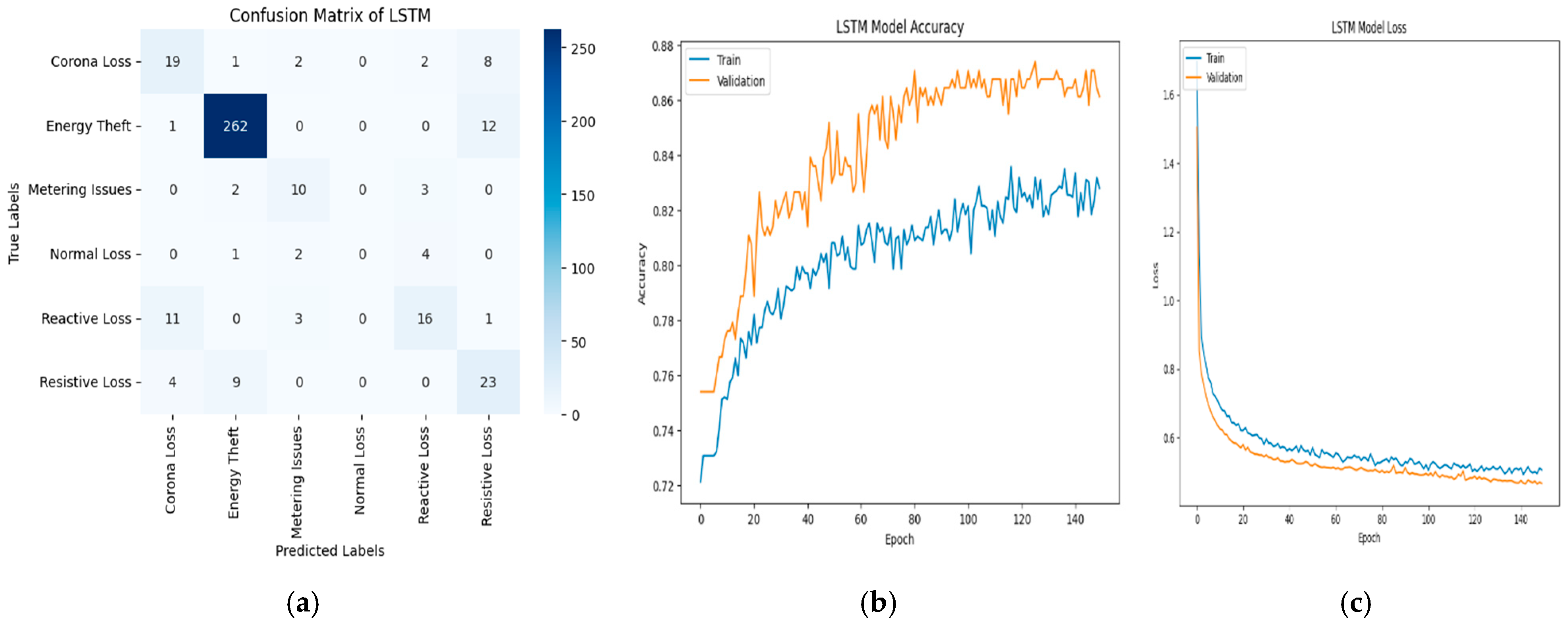
Confusion matrix: The confusion matrix is a tabular summary showing the number of correct and incorrect predictions for each class, organized by true labels (rows) and predicted labels (columns). While the elements of the main diagonal represent the number of correctly classified instances, the off-diagonal elements represent the number of misclassified instances. It matrix consists of four key components, namely,

• True Positive (TP), which indicates the number of positive cases that the model correctly identified;
• False Negative (FN), representing the number of actual positive cases that the model incorrectly classified as negative;
• False Positive (FP), which refers to the number of negative cases that the model mistakenly classified as positive;
• True Negative (TN), signifying the number of negative cases that the model correctly classified.

These components can be used to compute machines learning models as follows.

ii.

Accuracy: The accuracy of the classification system refers to the ratio of correctly classified instances (TP + TN) to the total number of instances (TP + TN + FP + FN). It can be mathematically expressed as Equation (33).

$$Accuracy={\displaystyle \frac{TP+TN}{(TP+FP+TN+FN)}}$$

(33)

It is usually measured in percentage, and the higher the value of the accuracy of a system, the better the system.

iii.

Recall: The recall is simply defined as the ratio of correctly predicted positive instances to all the actual positive instances. The idea behind the recall is how many instances have been classified as a particular class of losses. Recall is also called sensitivity, and it can be mathematically expressed as Equation (34).

$$Recall={\displaystyle \frac{TP}{(TP+FN)}}$$

(34)

Note also that a high recall value implies that the model is good at identifying the most positive instances.

iv.

F1-score: The F1-score is also known as the F Measure, and it measures the harmonic mean/equilibrium between the precision and the recall, thereby balancing their trade-off. It can be mathematically expressed as Equation (35).

$$F1-score={\displaystyle \frac{2\ast precision\ast recall}{precision+recall}}$$

(35)

Also, the higher the F1-score of a system, the better the balance between the precision and recall of the system.

v.

Precision: The precision of a classification system simply measures the ratio of correctly predicted positive instances to the total predicted positive instances. It can be mathematically expressed as Equation (36).

$$Precision={\displaystyle \frac{TP}{(TP+FP)}}$$

(36)

A higher precision value implies that the model is excellent at avoiding false positives.

3. Results and Discussions

The results, ranging from data analysis to model testing obtained in this study, are presented in this section.

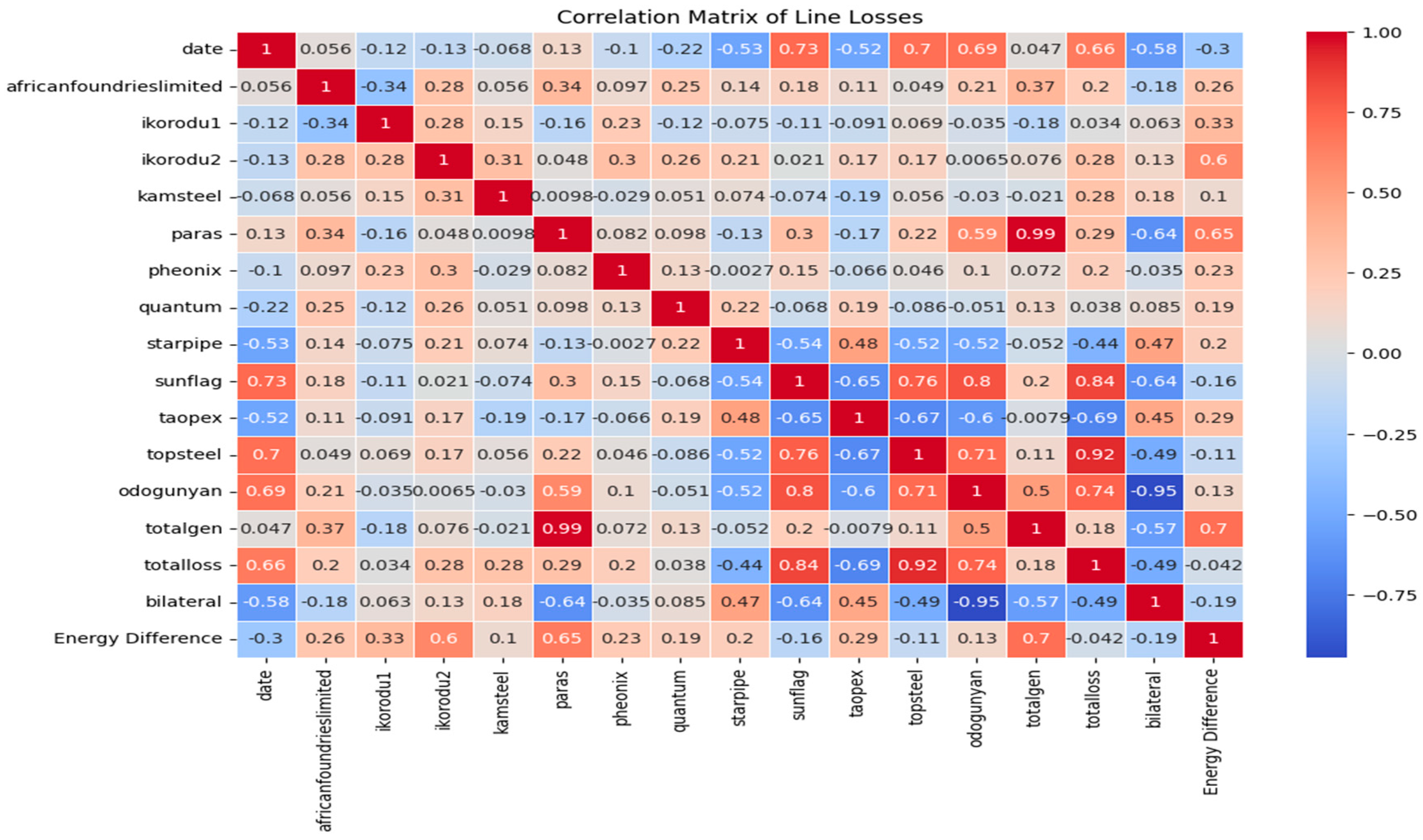
3.1. Insights from Data Preprocessing

Figure 7 presents a histogram illustrating the distribution of transmission losses for each line under consideration. The loss values for the African Foundries Limited line range approximately between 0 and 6, with a concentration around 4. This suggests that the line experiences consistent losses, which may be attributed to normal operational conditions or typical inefficiencies.

For the Ikorodu1 line, the loss values range between −60 and 20, with the majority of losses displaying a nearly normal distribution across the entire range. This indicates a varied range of losses, potentially resulting from fluctuating operational conditions. Similarly, the Ikorodu2 line shows loss values ranging from 0 to 150, with most of the losses normally distributed throughout the plot. The peak at 0 could represent periods of minimal usage or highly efficient operations. The Kamsteel line exhibits loss values between 0 and 16, with most data points concentrated near 0, indicating that lower losses dominate this dataset. In contrast, the Paras line displays a multimodal distribution, with prominent peaks near 0, between 60 and 80, and around 100–110. The wide range of this distribution (0 to 120) suggests significant variability in the system, which may be due to changing operational conditions or external factors.

For the Phoenix line, the distribution is positively skewed, with the majority of data points concentrated between 1 and 3. Losses beyond 6 are rare, suggesting occasional sporadic occurrences. The Quantum line, on the other hand, shows a sharp peak in the 0–5 range, with a right-skewed distribution and a notable drop in occurrences at higher loss values, indicating possible outliers or rare events. The Starpipe line demonstrates the highest concentration of data in the 0–0.5 range, with over 300 occurrences. As the loss value increases, the frequency of occurrences declines, with a wider distribution between 1 and 3. In the case of Sunflag, a dominant peak occurs in the 0–1 range, with over 1000 instances. A sharp decline is observed beyond this range, suggesting minimal variation in losses at higher values.

The Taopex line exhibits multiple peaks, notably near 0, at 10, and around 18–20, with instances exceeding 350. This suggests multiple operational conditions influencing the losses. The Topsteel line shows a similar trend, with the highest concentration of data in the 0–0.5 range, with over 1300 occurrences, indicating that most values in this dataset are either exactly 0 or very close to it. Finally, the Odogunyan line reveals a bimodal distribution, with peaks around values 20–30 and between 110 and 125. This suggests that the line experiences two distinct operational phases, each characterized by different loss behaviors. These results provide a clearer understanding of the system dynamics, offering insights into the causes of high variability in losses. Such information is crucial for improving system performance and aligning operational strategies with performance objectives.

Figure 8 displays the correlation matrix heatmap, which depicts the Pearson correlation coefficients between different lines, ranging from −1 to 1. A strong positive correlation is observed between the “totalgen” and “totalloss” lines, indicating a strong relationship between total generation and total losses. Additionally, a strong positive correlation is observed between “paras” and “totalgen”. In contrast, “starpipe” and “taopex” exhibit a strong negative correlation, suggesting an inverse relationship between these lines. The “Energy Difference” line shows moderate correlations with several other lines, highlighting its dependence on multiple factors. These findings are essential for understanding the factors affecting losses, optimizing energy transmission, and improving overall efficiency in power systems.

Figure 9 illustrates the time series analysis of daily average energy losses for total generation and total load in the system over the period from June 2024 to September 2024. The energy losses, expressed in megawatts (MW), exhibit significant fluctuations throughout the analyzed period, characterized by notable spikes and dips. The energy loss trend for the total load shows a relatively stable and gradual progression, with occasional minor peaks consistently remaining below 30 MW. In contrast, the daily average energy loss for total generation demonstrates substantial variations, with a particularly high energy loss observed at the beginning of June 2024, often exceeding 100 MW. This is followed by sharp declines and subsequent spikes, suggesting instability or inefficiency in generation. The sudden drops in energy loss observed in late June and mid-August 2024 are indicative of potential system outages or scheduled maintenance events, which contribute to these irregular fluctuations.

Figure 10 presents the distribution of energy losses for both total generation and total load within the network. The horizontal axis represents the magnitude of energy loss, ranging from approximately −20 MW to 140 MW, while the vertical axis displays the relative frequency of occurrence of these energy loss values, normalized to show the probability density rather than raw observations. The area under each curve sums to 1, offering insights into the overall behavior of the system. The distribution for total generation exhibits a bimodal shape, suggesting that generation losses are more variable and prone to extreme deviations. In contrast, the total load distribution is unimodal, with a prominent peak around 20 MW, indicating that load losses tend to be smaller and more consistent compared to generation losses. Additionally, there is a region of overlap between the two distributions, specifically around 40–60 MW, which implies that, in certain scenarios, generation and load losses may be of similar magnitude. The higher variability and greater magnitude of generation losses highlight that energy production is more susceptible to inefficiencies than the load side of the system.

The result presented in

Table 12. Statistical description of the line losses.

Statistic	AFL	I1	I 2	Ks	Ps	Phx	Qt	Sp	Sf	Tp	Ts	Ogy	TG	TL	Bl	ED
Mean	3.84	−23.16	78.52	2.52	69.40	2.95	2.56	1.31	4.25	7.24	7.26	45.56	76.64	24.69	−20.87	107.31
Min	0.00	−67.71	−1.37	0.00	0.00	0.00	0.00	0.00	0.00	−1.47	0.00	0.00	0.00	−100.18	−40.74	−40.74
25%	3.66	−32.54	69.89	0.00	43.19	2.21	2.30	0.39	0.42	1.01	0.80	19.12	55.62	12.76	−40.04	82.23
50% (Median)	4.04	−24.81	83.64	0.00	72.58	2.59	2.63	1.21	0.92	7.41	1.05	24.70	88.75	16.60	−10.20	113.91
75%	4.30	−15.34	93.49	3.18	96.50	3.49	2.93	2.00	7.16	11.90	16.93	82.70	104.71	39.72	−2.96	138.99
Max	6.58	25.81	128.60	17.87	114.41	12.27	21.51	3.68	21.60	21.88	44.60	129.59	117.85	68.51	54.39	218.97
Std Dev	0.87	15.12	24.80	4.23	36.14	1.64	1.01	0.96	6.01	5.81	10.13	42.25	35.62	15.71	32.30	45.60

shows the statistical description of the losses, offering insight into the distribution and spread of the losses obtained from the case study. It can be seen that AFL has a relatively small spread of loss values, ranging from 0 to 6.58, with a mean, maximum, minimum, and standard deviation of 3.84, 6.58, 0, and 0.87, respectively. Also, I1 has a wide spread of loss values, ranging from −67.71 to 25.81, with a mean, maximum, minimum, and standard deviation of −23.16, 25.81, −67.71, and 15.12, respectively. It was generally observed that the losses show wide variations, especially for lines such as I1, Ps, Ogy, and ED, with large standard deviations indicating a high spread, whereas some lines like Phx and Qt show relatively lower spread and variability.

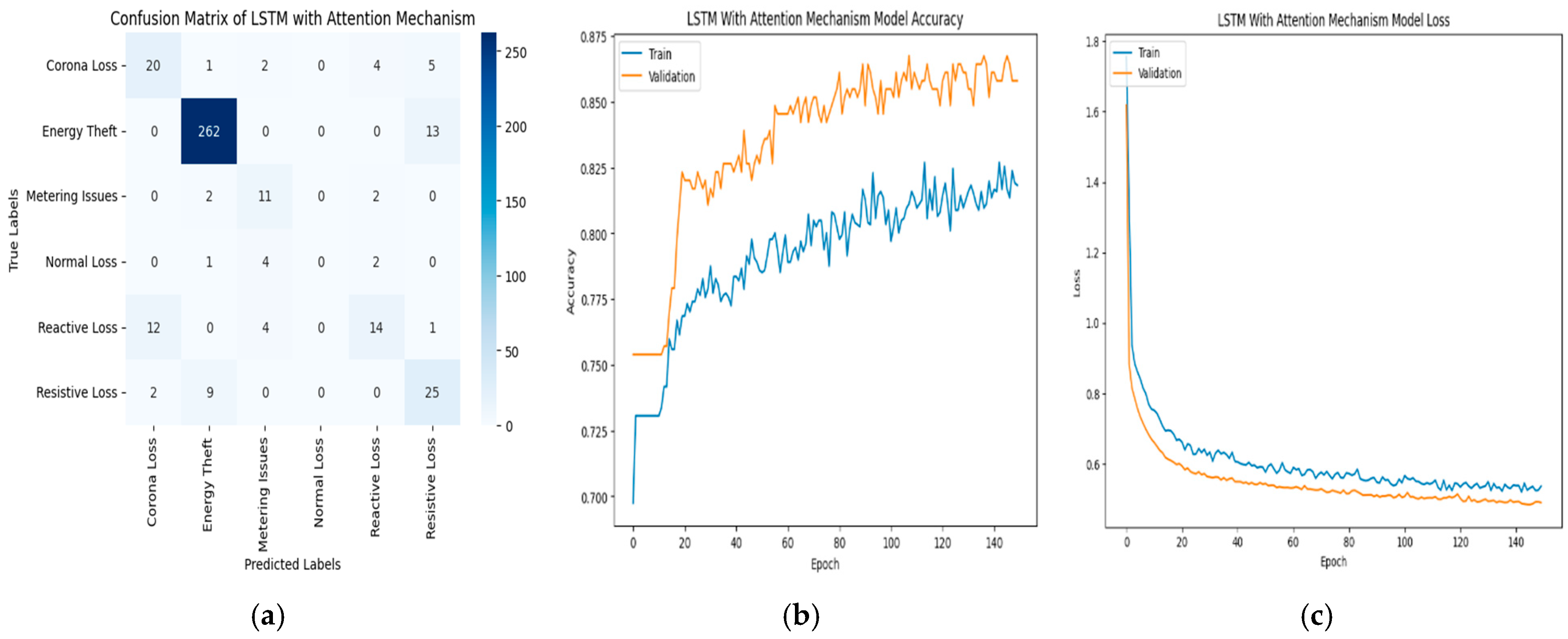
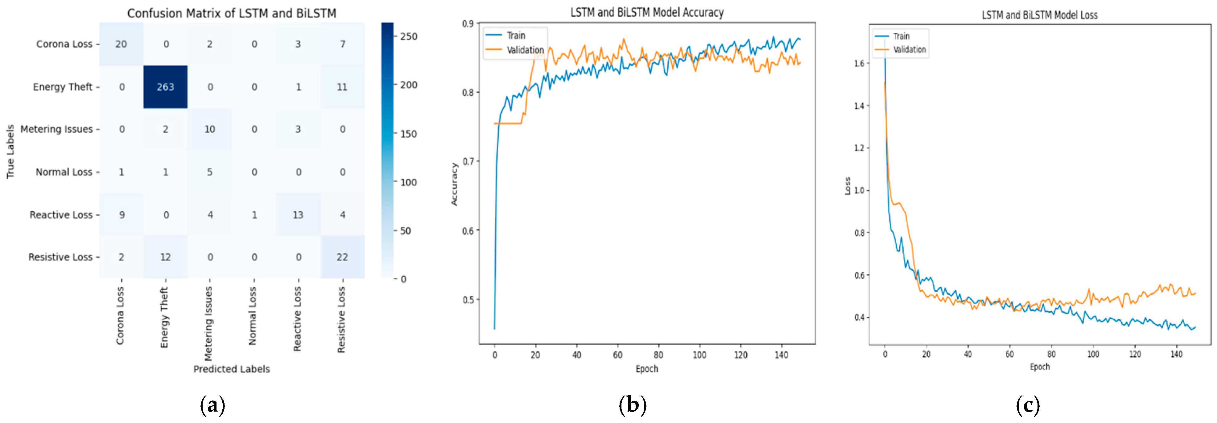
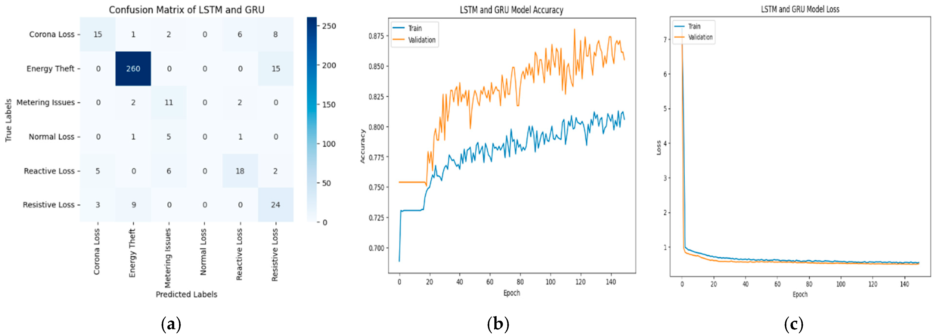
3.2. Transmission Loss Classification Result

As shown in

Table 13. Distribution of loss by type.

Loss Type	Count
Energy Theft	1440
Resistive Loss	169
Corona Loss	150
Reactive Loss	113
Metering Issues	79
Normal Loss	29
Total Counts	1980

, energy theft has the highest occurrence, with 1440 instances, while normal loss has the lowest occurrence, with only 29. All other loss types fall between these two extremes. This suggests that energy theft is the most significant contributor to losses in the network, and efforts should be focused on addressing it while also monitoring the other loss types. Figure 11 presents the scatter plot of energy losses in the transmission network, illustrating that the total loss for each data point ranges from approximately −50 MW to over 200 MW. The data points are categorized into six different loss types, each represented by a unique color.

Generally, it can be inferred that energy theft dominates the loss magnitude, indicating that it is the largest contributor to total losses. It is also evident that metering issues and normal loss are less frequent, with sparse occurrences suggesting they are less impactful. In conclusion, this result provides an effective means of visualizing the classification and magnitude of different loss types, highlighting the significant impact of energy theft.

Figure 12 presents a confusion matrix for evaluating the performance of the LSTM-based classification model for predicting six different loss types. It can be observed from the model that there were 19, 262, 10, 0, 16, and 23 correct classifications of corona loss, energy theft, metering issues, normal loss, reactive loss, and resistive loss, respectively. Additionally, the LSTM validation accuracy and training accuracy start at about 0.750 and 0.720, respectively, and increase steadily, though with significant fluctuations, which implies the LSTM’s ability to learn from the training. Similarly, the training loss and validation loss start at a high value of approximately 1.7 and decrease continuously until they reach approximately 0.5 by the end of the training process.

Figure 13 shows the result of the LSTM-AM model with a confusion matrix, where it is observed that there were 20, 262, 11, 0, 14, and 25 correct classifications of corona loss, energy theft, metering issues, normal loss, reactive loss, and resistive loss, respectively. The validation accuracy and training accuracy start at about 0.755 and 0.700, respectively, and increase steadily with fluctuations, which implies the model’s ability to learn from the training process. Similarly, the training loss and validation loss start at a high value of approximately 1.7 and decrease continuously until they reach approximately 0.4 by the end of the training process.

Figure 14 depicts the result of BiLSTM, where the confusion matrix reported that 21, 262, 11, 0, 20, and 22 correct classifications of corona loss, energy theft, metering issues, normal loss, reactive loss, and resistive loss, respectively, were obtained. For the model accuracy, the validation and training initiate at about 0.750 and 0.650, respectively, and increase steadily with fluctuations, which implies the model’s ability to learn from the training process. Likewise, for the model loss, the training and validation initiate at approximately 1.6 and 1.3, respectively, but decrease sharply to about 0.5 at 20 epochs and continue until they reach approximately 0.4 by the end of the training process.

Figure 15 depicts the result of the GRU model, with the confusion matrix reporting that 20, 260, 11, 0, 17, and 21 correct classifications of corona loss, energy theft, metering issues, normal loss, reactive loss, and resistive loss, respectively, were obtained. The model accuracy and model loss of the GRU exhibit the same trend as that of BiLSTM.

Figure 16 presents the result of LSTM-BiLSTM, where the confusion matrix reported that 20, 263, 10, 0, 13, and 22 correct classifications of corona loss, energy theft, metering issues, normal loss, reactive loss, and resistive loss, respectively, were obtained. For the model accuracy, the validation and training begin at about 0.750 and 0.450, respectively, and increase steadily with fluctuations, indicating the model’s ability to learn from the training process. Similarly, for the model loss, the training and validation initiate at approximately 1.7 and 1.5, respectively, but decrease sharply to about 0.5 at 20 epochs and continue until the end of the training process.

Figure 17 presents a confusion matrix for evaluating the performance of the LSTM-GRU-based classification model for predicting six different loss types. It can be observed from the model that there were 15, 260, 11, 0, 18, and 24 correct classifications of corona loss, energy theft, metering issues, normal loss, reactive loss, and resistive loss, respectively. For the model accuracy, the validation and training start at about 0.750 and 0.675, respectively, and increase steadily with fluctuations, depicting the model’s ability to learn from the training process. Additionally, for the model loss, the training and validation start at approximately 1.7 and 1.5, respectively, but decrease sharply to about 0.5 at 20 epochs and continue until the end of the training process.

The results presented in

Table 14. Comparison of LSTM with Models for Classification of Transmission Losses.

Model	Accuracy (%)	Precision	Recall	F1-Score
LSTM	83.33	0.83	0.83	0.83
LSTM-AM	83.84	0.54	0.58	0.55
BiLSTM	82.07	0.83	0.84	0.83
GRU	83.08	0.83	0.83	0.83
LSTM & BiLSTM	82.83	0.82	0.83	0.82
LSTM & GRU	82.83	0.83	0.83	0.82

compare the accuracy of various loss models applied to the case study. The table reports the performance of six different models: LSTM, LSTM-AM, BiLSTM, GRU, LSTM-BiLSTM, and LSTM-GRU, which are formed from various combinations of Long Short-Term Memory (LSTM), Gated Recurrent Units (GRU), and Attention Mechanism (AM). The accuracy values for these models are as follows: 83.33% for LSTM, 83.84% for LSTM-AM, 82.07% for BiLSTM, 83.08% for GRU, 82.83% for LSTM-BiLSTM, and 82.83% for LSTM-GRU. Based on these results, it can be inferred that the LSTM-AM model achieves the highest accuracy, indicating that higher accuracy is desirable for optimal system performance.

Furthermore, the precision values for the models are reported as follows: 0.83 for LSTM, 0.54 for LSTM-AM, 0.83 for BiLSTM, 0.83 for GRU, 0.82 for LSTM-BiLSTM, and 0.83 for LSTM-GRU. Among these, the models LSTM, BiLSTM, GRU, and LSTM-GRU demonstrate superior precision, as values closer to unity signify better precision. In terms of recall, the values are as follows: 0.83 for LSTM, 0.58 for LSTM-AM, 0.84 for BiLSTM, 0.83 for GRU, 0.83 for LSTM-BiLSTM, and 0.83 for LSTM-GRU. BiLSTM stands out with the highest recall, which reflects better performance in correctly identifying relevant instances (with values approaching unity indicating better recall). Finally, the F1-scores for each model are: 0.83 for LSTM, 0.55 for LSTM-AM, 0.83 for BiLSTM, 0.83 for GRU, 0.82 for LSTM-BiLSTM, and 0.82 for LSTM-GRU. The F1-scores suggest that LSTM, BiLSTM, and GRU perform better, with higher F1-scores indicating a balanced trade-off between precision and recall.

These results indicate that the integration of the attention mechanism (AM) slightly enhances the LSTM performance for the transmission loss management system. Notably, the hybridization of LSTM and GRU results in a lower accuracy of 82.83%, which is comparatively less effective than the other hybrid models. In conclusion, while the standalone models GRU and LSTM performed well, the hybrid LSTM-AM model yielded the best results, underscoring the importance of combining different models to achieve higher accuracy. Figure 18 visually represents the results presented in Table 10, further illustrating that the hybrid LSTM-AM model provided the best performance, while BiLSTM achieved the lowest performance. Based on these findings, it is recommended that hybridizing deep learning models for feature extraction, combined with machine learning models for classification, be adopted to enhance the performance of the transmission loss management system.

The comparison of the present study with existing studies is presented in

Table 15. Comparison with existing studies.

Authors	Focus	Models	Results
[41]	Transmission line fault classification (Jamshoro-New Karachi), Sindh, Pakistan	Temporal convolutional networks (TCN) Bidirectional Long Short-Term Memory (BiLSTM) Gated Recurrent Units (GRUs)	TCN achieves accuracy of 99.9%. BiLSTM achieves accuracy of 92.31% GRU achieves accuracy of 95.27%.
[42]	Fault detection and location power grid	Artificial neural network (ANN) Adaptive Neuro-fuzzy inference system (ANFIS)	ANN recorded 92–95% operational efficiency ANFIS recorded 97–99% operational efficiency
[43]	Fault classification in 115-kV hybrid transmission line in the Provincial Electricity Authority (PEA-Thailand) system	Probabilistic neural networks (PNNs) Back-propagation neural networks (BPNNs) Support vector machine (SVM)	PNN recorded 100% accuracy of sending end BPNN recorded 100% accuracy of sending end SVM recorded 100% accuracy of sending end
Present Study	Transmission line loss classification	Long short-term memory (LSTM) Bidirectional long short-term memory (BiLSTM) Gated recurrent units (GRU) Long short-term memory—Attention Mechanism (LSTM-AM) LSTM-BiLSTM LSTM-GRU	LSTM achieved accurcay of 83.33% BiLSTM achieved accurcay of 82.07% GRU achieved accurcay of 83.08% LSTM-AM achieved accurcay of 83.84% LSTM-BiLSTM achieved accurcay of 82.83% LSTM-GRU achieved accurcay of 82.83%

. It can be observed that while existing studies focused chiefly on transmission line faults detection and classification this study focused on transmission line loss classification. This establish the novelty of this study with a focus on transmission line loss classification. It should be noted that both the existing studies and the present study leverages deep models for the purpose of classification.

4. Conclusions and Future Directions

This study was driven by the inefficiencies inherent in traditional methods of managing transmission losses, which prompted the exploration of artificial intelligence (AI) as a potential solution. The findings highlight the pivotal role of data preprocessing and feature engineering as diagnostic tools, facilitating the identification of patterns, inefficiencies, and correlations within energy system operations. These techniques emphasize the importance of optimizing generation processes to reduce the high variability and magnitude of transmission losses while maintaining stable and manageable load losses.

Statistical analysis of transmission loss data revealed significant variations, particularly for lines such as I1, Ps, Ogy, and ED, where large standard deviations indicated a broad spread of values. The extreme fluctuations observed in the maximum and minimum values of several variables suggested the presence of outliers, highlighting the need for targeted strategies to minimize losses and enhance system efficiency. In evaluating the performance of seven different classification scenarios, it was found that standalone models—GRU and LSTM—performed well, while BiLSTM showed the least favorable results. Notably, the hybrid LSTM-AM model outperformed all others, achieving the highest classification accuracy of 83.84%. This positions LSTM-AM as the most effective architecture for transmission loss management. Although the accuracy of the models ranged from 82.07% to 83.84%, the hybrid LSTM-BiLSTM and LSTM-GRU models both reached 82.83%, indicating that combining these architectures did not lead to a significant accuracy improvement.

The study provides important findings and practical recommendations. Given the strong performance of the hybrid LSTM-AM model, it is recommended that future transmission loss classification systems adopt hybrid approaches that combine deep learning for feature extraction with machine learning techniques for prediction. However, it is important to acknowledge the study’s limitations, particularly the unavailability of comprehensive transmission loss data from the Nigerian grid. This lack of data presented a challenge in fully optimizing the model’s performance. Similarly, the lack of data limits the study to a particular section of the entire Nigerian transmission network under consideration.

Looking ahead, future work will focus on exploring the optimization potential of the Particle Swarm Optimization (PSO) algorithm to reduce energy losses in the transmission system. This approach aims to further enhance system efficiency and maximize revenue by minimizing transmission losses. Additionally, future studies may seek to expand the dataset to strengthen model robustness and improve performance across diverse real-world scenarios.

References

1. Amole, A.O.; Oladipo, S.; Olabode, O.E.; Makinde, K.A.; Gbadega, P. Analysis of grid/solar photovoltaic power generation for improved village energy supply: A case of Ikose in Oyo State Nigeria. Renew. Energy Focus 2023, 44, 186–211. [Google Scholar] [CrossRef]
2. Gaonwe, T.P.; Kusakana, K.; Hohne, P.A. A review of solar and air-source renewable water heating systems, under the energy management scheme. Energy Rep. 2022, 8, 1–10. [Google Scholar] [CrossRef]
3. Ma, Z.; Ye, C.; Li, H.; Ma, W. Applying support vector machines to predict building energy consumption in China. Energy Procedia 2018, 152, 780–786. [Google Scholar] [CrossRef]
4. Kiasari, M.; Ghaffari, M.; Aly, H.H. A Comprehensive Review of the Current Status of Smart Grid Technologies for Renewable Energies Integration and Future Trends: The Role of Machine Learning and Energy Storage Systems. Energies 2024, 17, 4128. [Google Scholar] [CrossRef]
5. Akinyele, D.; Amole, A.; Olabode, E.; Olusesi, A.; Ajewole, T. Simulation and analysis approaches to microgrid systems design: Emerging trends and sustainability framework application. Sustainability 2021, 13, 11299. [Google Scholar] [CrossRef]
6. Amole, A.O.; Akinyele, D.O.; Olabode, O.E.; Idogun, O.O.; Adeyeye, A.O.; Olarotimi, B.S. Comparative Analysis of Techno-Environmental Design of Wind and Solar Energy for Sustainable Telecommunications Systems in Different Regions of Nigeria. Int. J. Renew. Energy Res. 2021, 11, 1776–1792. [Google Scholar] [CrossRef]
7. Adefarati, T.; Bansal, R.C. Integration of renewable distributed generators into the distribution system: A review. IET Renew. Power Gener. 2016, 10, 873–884. [Google Scholar] [CrossRef]
8. Ehimen Airoboman, A. On the Assessment of Power System Stability Using Matlab/Simulink Model. Int. J. Energy Power Eng. 2015, 4, 51. [Google Scholar] [CrossRef]
9. Salimon, S.A.; Fajinmi, I.O.; Adewuyi, O.B.; Pandey, A.K.; Adebiyi, O.W.; Kotb, H. Graph theory-enhanced integrated distribution network reconfiguration and distributed generation planning: A comparative techno-economic and environmental impacts analysis. Clean. Eng. Technol. 2024, 22, 100808. [Google Scholar] [CrossRef]
10. Owusu, K.B.; Annan, J.K.; Effah, E.; Kwame Tweneboah-Koduah, F.; Bediako Owusu, K.; Kojo Annan, J. Mitigation of Technical Losses in Ghana’s Transmission Network using Optimal Capacitor Bank Allocation Technique. Glob. J. Res. Eng. Felectrical Electron. Eng. 2015, 15, 21–31. [Google Scholar]
11. Alam, M.S.; Arefifar, S.A. Hybrid PSO-TS Based Distribution System Expansion Planning for System Performance Improvement Considering Energy Management. IEEE Access 2020, 8, 221599–221611. [Google Scholar] [CrossRef]
12. Oyedepo, S.O.; Uwoghiren, T.; Babalola, P.O.; Nwanya, S.C.; Kilanko, O.; Leramo, R.O.; Aworinde, A.K.; Adekeye, T.; Oyebanji, J.A.; Abidakun, O.A. Assessment of Decentralized Electricity Production from Hybrid Renewable Energy Sources for Sustainable Energy Development in Nigeria. Open Eng. 2019, 9, 72–89. [Google Scholar] [CrossRef]
13. Carr, D.; Thomson, M. Non-Technical Electricity Losses. Energies 2022, 15, 2218. [Google Scholar] [CrossRef]
14. Gaur, B.; Ucheniya, R.; Saraswat, A. Real power transmission loss minimization and bus voltage improvement using UPFC. In Lecture Notes in Electrical Engineering; Springer: Berlin/Heidelberg, Germany, 2020; Volume 662, pp. 1–9. [Google Scholar]
15. Kojima, M.; Trimble, C. Making Power Affordable for Africa and Viable for Its Utilities; World Bank: Washington, DC, USA, 2016. [Google Scholar]
16. de Savian, F.S.; Siluk, J.C.M.; Garlet, T.B.; Do Nascimento, F.M.; Pinheiro, J.R.; Vale, Z. Non-technical Losses in Brazil: Overview, Challenges, and Directions for Identification and Mitigation. Int. J. Energy Econ. Policy 2022, 12, 93–107. [Google Scholar] [CrossRef]
17. Barja-Martinez, S.; Aragüés-Peñalba, M.; Munné-Collado, Í.; Lloret-Gallego, P.; Bullich-Massagué, E.; Villafafila-Robles, R. Artificial intelligence techniques for enabling Big Data services in distribution networks: A review. Renew. Sustain. Energy Rev. 2021, 150, 111459. [Google Scholar] [CrossRef]
18. Kim, S.; Sun, Y.; Lee, S.; Seon, J.; Hwang, B.; Kim, J.; Kim, J.; Kim, K.; Kim, J. Data-Driven Approaches for Energy Theft Detection: A Comprehensive Review. Energies 2024, 17, 3057. [Google Scholar] [CrossRef]
19. Alzahrani, A.; Ferdowsi, M.; Shamsi, P.; Dagli, C.H. Modeling and Simulation of Microgrid. Procedia Comput. Sci. 2017, 114, 392–400. [Google Scholar] [CrossRef]
20. Khan, F.A.; Pal, N.; Saeed, S.H. Optimization and sizing of SPV/Wind hybrid renewable energy system: A techno-economic and social perspective. Energy 2021, 233, 121114. [Google Scholar] [CrossRef]
21. Guarda, F.G.K.; Hammerschmitt, B.K.; Capeletti, M.B.; Neto, N.K.; dos Santos, L.L.C.; Prade, L.R.; Abaide, A. Non-Hardware-Based Non-Technical Losses Detection Methods: A Review. Energies 2023, 16, 2054. [Google Scholar] [CrossRef]
22. Viegas, J.L.; Esteves, P.R.; Vieira, S.M. Clustering-based novelty detection for identification of non-technical losses. Int. J. Electr. Power Energy Syst. 2018, 101, 301–310. [Google Scholar] [CrossRef]
23. Saeed, M.S.; Mustafa, M.W.; Hamadneh, N.N.; Alshammari, N.A.; Sheikh, U.U.; Jumani, T.A.; Khalid, S.B.A.; Khan, I. Detection of non-technical losses in power utilities—A comprehensive systematic review. Energies 2020, 13, 4727. [Google Scholar] [CrossRef]
24. Odje, M.; Uhunmwangho, R.; Okedu, K.E. Aggregated Technical Commercial and Collection Loss Mitigation Through a Smart Metering Application Strategy. Front. Energy Res. 2021, 9, 703265. [Google Scholar] [CrossRef]
25. Iheukwumere Uchechukwu, M.; Ephraim, O.N.C. Evaluation of Technical and Commercial Losses on Power Distribution Networks in Nigeria Using Statistical Analytical Method. Am. J. Electr. Comput. Eng. 2021, 5, 56. [Google Scholar] [CrossRef]
26. Kumar, M.; Pal, N. Machine Learning-based Electric Load Forecasting for Peak Demand Control in Smart Grid. Comput. Mater. Contin. 2023, 74, 4785. [Google Scholar] [CrossRef]
27. Ahmadi, B.; Giraldo, J.S.; Hoogsteen, G.; Gerards, M.E.T.; Hurink, J.L. A multi-objective decentralized optimization for voltage regulators and energy storage devices in active distribution systems. Int. J. Electr. Power Energy Syst. 2023, 153, 109330. [Google Scholar] [CrossRef]
28. Passos Júnior, L.A.; Oba Ramos, C.C.; Rodrigues, D.; Pereira, D.R.; de Souza, A.N.; Pontara da Costa, K.A.; Papa, J.P. Unsupervised non-technical losses identification through optimum-path forest. Electr. Power Syst. Res. 2016, 140, 413–423. [Google Scholar] [CrossRef]
29. Guha, D.; Roy, P.K.; Banerjee, S. Symbiotic organism search algorithm applied to load frequency control of multi-area power system. Energy Syst. 2018, 9, 439–468. [Google Scholar] [CrossRef]
30. Bartłomiejczyk, M.; Hołyszko, P.; Filipek, P. Measurement and analysis of transmission losses in the supply system of electrified transport. J. Ecol. Eng. 2016, 17, 64–71. [Google Scholar] [CrossRef]
31. Xie, J.; Lu, Y.; Gao, R.; Zhu, S.C.; Wu, Y.N. Cooperative Training of Descriptor and Generator Networks. IEEE Trans. Pattern Anal. Mach. Intell. 2020, 42, 27–45. [Google Scholar] [CrossRef]
32. Velasco, J.A.; Amaris, H.; Alonso, M. Deep Learning loss model for large-scale low voltage smart grids. Int. J. Electr. Power Energy Syst. 2020, 121, 106054. [Google Scholar] [CrossRef]
33. Coma-Puig, B.; Calvo, A.; Carmona, J.; Gavaldà, R. A case study of improving a non-technical losses detection system through explainability. Data Min. Knowl. Discov. 2024, 38, 2704–2732. [Google Scholar] [CrossRef]
34. Almasoudi, F.M. Enhancing Power Grid Resilience through Real-Time Fault Detection and Remediation Using Advanced Hybrid Machine Learning Models. Sustainability 2023, 15, 8348. [Google Scholar] [CrossRef]
35. Shafei, A.P.; Silva, J.F.A.; Monteiro, J. Convolutional neural network approach for fault detection and characterization in medium voltage distribution networks. E-Prime-Adv. Electr. Eng. Electron. Energy 2024, 10, 100820. [Google Scholar] [CrossRef]
36. Chamangard, M.; Ghodrati Amiri, G.; Darvishan, E.; Rastin, Z. Transfer Learning for CNN-Based Damage Detection in Civil Structures with Insufficient Data. Shock Vib. 2022, 2022, 3635116. [Google Scholar] [CrossRef]
37. Yin, X.; Zuo, Y.; Fu, G. Design of intelligent detection method for electricity transmission line equipment defect based on data mining algorithm. Int. J. Thermofluids 2024, 24, 100814. [Google Scholar] [CrossRef]
38. Khan, A.Q.; Ullah, Q.; Sarwar, M.; Gul, S.T.; Iqbal, N. Transmission Line Fault Detection and Identification in an Interconnected Power Network using Phasor Measurement Units. IFAC-Pap. 2018, 51, 1356–1363. [Google Scholar] [CrossRef]
39. Amole, A.O.; Oladipo, S.; Ighravwe, D.; Makinde, K.A.; Ajibola, J. Comparative Analysis of Deep Learning Techniques Based COVID-19 Impact Assessment on Electricity Consumption in Distribution Network. Niger. J. Technol. Dev. 2023, 20, 29–46. [Google Scholar] [CrossRef]
40. Sehovac, L.; Nesen, C.; Grolinger, K. Forecasting building energy consumption with deep learning: A sequence to sequence approach. In Proceedings of the Proceedings-2019 IEEE International Congress on Internet of Things, ICIOT 2019-Part of the 2019 IEEE World Congress on Services, Milan, Italy, 8–13 July 2019; Institute of Electrical and Electronics Engineers Inc.: Piscataway Township, NJ, USA, 2019; pp. 108–116. [Google Scholar]
41. Tunio, N.A.; Tunio, M.A.; Raza, M.A.; Faheem, M.; Hashmani, A.A.; Nadeem, R. Performance Comparison Between Deep Learning Models for Fault Classification in Transmission Lines Using Time Series Data. Energy Sci. Eng. 2025, 6, 2330–2351. [Google Scholar] [CrossRef]
42. Yadav, G.K.; Kirar, M.K.; Gupta, S.C.; Rajender, J. Integrating ANN and ANFIS for effective fault detection and location in modern power grid. Sci. Technol. Energy Transit. 2025, 80, 1–20. [Google Scholar] [CrossRef]
43. Klomjit, J.; Ngaopitakkul, A. Comparison of artificial intelligence methods for fault classification of the 115-kv hybrid transmission system. Appl. Sci. 2020, 10, 3967. [Google Scholar] [CrossRef]
Figure 1. Ikorodu–Sagamu 132kV Double Circuit Line.
Energies 18 02742 g001
Figure 2. The equivalent circuit of a transmission line.
Energies 18 02742 g002
Figure 3. The architecture of LSTM Unit.
Energies 18 02742 g003
Figure 4. The architecture of BiLSTM Unit.
Energies 18 02742 g004
Figure 5. The architecture of GRU Unit.
Energies 18 02742 g005
Figure 6. Flowchart of the transmission loss classification system.
Energies 18 02742 g006
Figure 7. Distribution of losses for the lines under consideration.
Energies 18 02742 g007
Figure 8. Correlation of the line losses.
Energies 18 02742 g008
Figure 9. Time series of total generation and total loss.
Energies 18 02742 g009
Figure 10. Distribution of energy loss for total generation and total loss.
Energies 18 02742 g010
Figure 11. Classification of loss types.
Energies 18 02742 g011
Figure 12. LSTM model result.
Energies 18 02742 g012
Figure 13. LSTM-AM model results.
Energies 18 02742 g013
Figure 14. BiLSTM model result.
Energies 18 02742 g014
Figure 15. GRU model results.
Energies 18 02742 g015
Figure 16. LSTM-BiLSTM model result.
Energies 18 02742 g016
Figure 17. LSTM-GRU model results.
Energies 18 02742 g017
Figure 18. Comparison of Transmission Loss Classification Models.
Energies 18 02742 g018