Efficiency Testing of Pelton Turbines with Artificial Defects—Part 1: Buckets

Abstract

Pelton turbines are susceptible to hydro-abrasive erosion from sediment-laden flows, resulting in a progressive loss of efficiency. Typical defect classes can be derived from the analysis of such damage observed in hydropower plants. A systematic strategy was developed to investigate the effect of locally damaged Pelton runners on the efficiency in laboratory tests using a model turbine. For this purpose, nine identical runners were fabricated and machined with an increasing size, depth, or number of different artificial defect types, such as splitter, rounded or sharp-edged, defects at the cutout, defects in the bucket base, and added ripples on the bucket sides. The processing steps, the efficiency measurement, and the extracted slopes of the efficiency drops are discussed in detail. The main findings are that the efficiency losses due to the various defects increase in a good approximation linearly with the machining depth and that the individual defect types can be superimposed. Defects at the splitter, bucket base, and bucket side dominate the losses at partial load of the turbine, while those at the cutout dominate at full load. Based on the results of this measurement campaign, power plant operators can estimate the magnitude of efficiency losses in their plant.

1. Introduction

It is well known that Pelton turbines, especially at high heads, are susceptible to erosion due to sediment-laden flows. A large number of publications on this subject are summarized in comprehensive review articles [1,2]. Hydro-abrasive erosion progresses rapidly or slowly, depending on head and sediment load, and inevitably alters the surface of the turbine components, which in turn affects the local flow conditions. Typical damages found in Pelton turbines are erosion of the injector surfaces, especially at the seat ring and the needles, and erosion of the bucket surfaces, the crest of the splitter, and the cutout [3]. Hydro-abrasive erosion is inevitably associated with loss of power and revenue reduction. Based on a careful economic analysis, plant operators must decide when to repair, refurbish, or eventually replace their runners. This decision depends on many factors such as repair costs, turbine downtime, and electricity price trends [4,5,6,7].

Many studies in the past have attempted to correlate suspended sediment concentration and particle size distribution with the observed damage in buckets and injectors of Pelton turbines [3,8,9,10]. Defects have been quantified as mass loss [11,12] or deviations from templates [13,14,15], or by digitizing the bucket surfaces with, e.g., photogrammetry or laser scans [16,17]. A method for measuring the reduction in coating thickness of coated buckets due to hydro-abrasive erosion is presented in [8]. Among the many publications in the field, only a few studies establish a relationship between geometric defects and efficiency losses [8,9,10,11,14,18,19,20,21]. Most of the quantitative data on the relationship between geometric degradation and efficiency losses are available with respect to splitter height or width [18,21]. The drawback of such studies in hydropower plants is that there is always a sum of different defects that cannot be individually traced back to their effect on efficiency. Despite the common occurrence of typical defects on the splitter, cutout, or bucket surfaces, the individual defects will develop differently depending on the bucket design and the operating regime of the turbine. This lack of knowledge about the influence of the individual defects on efficiency is addressed in the present study. While accurate efficiency measurements in hydropower plants or index tests with good repeatability are always challenging, require personal experience, and involve a considerable financial outlay, the geometric degradation of elements in Pelton turbines can be easily documented and quantitatively measured using templates, scales, or laser scans [21]. For this reason, it would be desirable to be able to estimate the efficiency losses of typical geometric defects found in Pelton turbines. The ultimate goal of such estimates is, of course, the economic optimization of turbine refurbishment measures, which, however, is not part of this study.

To address the issue of efficiency losses associated with damage to the Pelton buckets due to erosion, a measuring campaign was initiated by the Lucerne School of Engineering and Architecture. After analyzing typical damages described in the literature [3,8,9,10,11,14,21] and in reports of hydropower plant operators, it was decided to perform tests with increasing artificial defects of the buckets. This approach allows the impact of each individual defect on efficiency to be evaluated separately or in combination. The stepwise increase in depth and size of the artificial defects enables the visualization of the drop in efficiency as a function of the abrasion progression of each defect considered individually over a wide range of the operating field. By combining defects, it is possible to determine whether and how individual damage patterns influence one another. In this way, the validity of the superposition principle of individual defects on efficiency can be verified. Furthermore, the issue of the progression of efficiency losses with increasing defects, as raised by [19,20,22], can be addressed.

Tests with suspended sediment in the laboratory, as presented in [23], were not considered feasible due to the long duration of the erosion process and the degradation of the sharp edges of the particles over time and thus their erosive effectiveness. Such investigations are valuable for understanding the erosion process and for validating numerical schemes for predicting erosion, but do not allow for an understanding of the effect of individual defects on efficiency, nor a prediction of efficiency losses of real turbines in the field.

To allow later validation of the efficiency losses with CFD (Computational Fluid Dynamics) simulations, the geometrical defects described in the present study were modeled with 3D-CAD (Computer-Aided Design). The modifications of the bucket geometries were modeled with as few geometrical parameters as possible to make them easily applicable for parameter studies. Simple parameterization also makes it easier to compare different bucket sizes and designs, especially regarding the determination of efficiency losses. Of course, such modeling of artificial defects involves many simplifications; e.g., the often-observed typical waviness of eroded splitter crests was not modeled.

In recent years, great progress has been made in the simulation of erosion processes using CFD. Local hotspots of erosion in Pelton buckets [24], injectors [25], and distributors [26] can be accurately predicted. However, the relationship between efficiency loss and simulated erosion patterns has not yet been established. The experimental data presented here will later allow the improvement of CFD simulation techniques based on validation with well-defined geometrical defects and accurate efficiency data.

2. Test Rig and Data Acquisition

2.1. Experimental Setup

The test rig comprises an alimentation pump feeding a single-jet horizontal model Pelton turbine, see Figure 1. The injector is equipped with an internal servomotor, the nozzle-needle angles are 90–50° and the nozzle diameter is 36.6 mm. The electromagnetic flow meter was calibrated before and after the test series using the flying start-and-finish method according to [27].

All boundary conditions for high-quality measurements required by the test standard [28], such as turbine size and test head, were met, see

Table 1. Hydraulic and geometrical parameters.

Turbine Part	Subject	Value
Hydraulic parameters	Head, H	120 m
	Flow rate, Q	11–35 L/s
	Nozzle seat ring diameter, D0	36.6 mm
Injector	Nozzle seat ring angle, αD	90°
	Needle angle, αN	50°
	Needle stroke, s	29 mm (0 to 35 L/s)
Runner	Jet pitch circle diameter, D	327.7 mm
	Inner bucket width, B	80 mm
	Lever arm for weights, rweight	1 m
Torque measurement	Lever arm for load cell generator, rgen	1 m
	Lever arm for load cell bearing, rbearing	0.25 m

. The shaft torque was measured using the principle of the balance arrangement, as described in (Section 7.4.2, [28]). The torque acting on the runner was measured at the torque arms of the swinging frames of the generator and the bearing block. The latter enables the frictional torque in the runner bearings to be determined.

The main counter-torque on the lever arm of the generator was generated by adding weights, m_weight, in the range of 2 to 24 kg. The residual torque was measured with a load cell, see Figure 2, left. This load cell had been calibrated with weights and displays kg, m_gen. The friction torque on the bearing is an order of magnitude smaller than that on the generator. Therefore, it was measured only with a load cell (in kg) and a shorter lever arm, m_bear, see Figure 2, right.

For data acquisition of each measuring point, data were sampled with a frequency of 1 or 2 kHz. Appropriate filtering was applied beforehand on each signal. The duration for each measuring point was set to 60 s. After internal averaging, n = 120 data points were read out every 0.5 s.

In addition to the efficiency measurements, endoscopic flow visualization was performed with cameras above and below the entering jet to observe splashing water due to artificial bucket defects.

2.2. Hydraulic Efficiency and Uncertainty Analysis

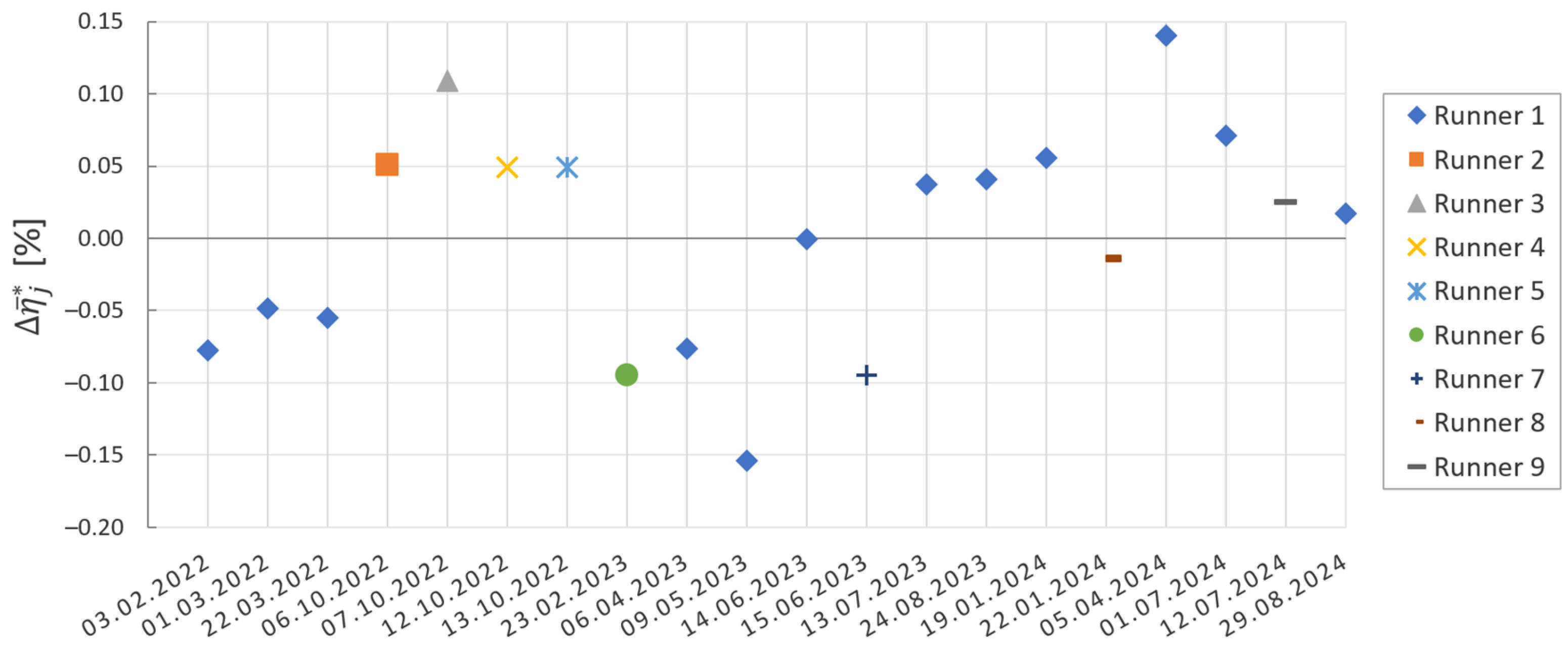
Measurements and data evaluation were performed according to [28]. The hydraulic efficiency is defined by the ratio of mechanical and hydraulic power (Section 8.3.3, [28]).

$${\eta }_h={\displaystyle \frac{P_m}{P_h}}$$

(1)

From the measured data points as described in Section 2.1, the mean values as well as the standard deviation of each quantity X were determined.

$$\overline{X}={\displaystyle \frac{{\sum }_{i=1}^n{X}_i}{n}} s_X=\sqrt{{\displaystyle \frac{{\sum }_{i=1}^n\left(X_i-\overline{X}\right)}{n-1}}}$$

(2)

The uncertainty in the measurement of a quantity X may be expressed as an absolute value e_X or as a relative value: f_X = e_X/X, [28], Annex F. In order to determine the total uncertainty of each measured quantity, the systematic and the random contributions have to be considered. All calculated uncertainties are listed in

Table 2. Uncertainties.

Uncertainty Type	Symbol	Error	Unit
Instrument uncertainties
Flow rate	${\left(f_Q\right)}_s$	±0.106	%
Pressure	${\left(e_{p_1}\right)}_s$	±900	Pa
Rotational speed	${\left(f_n\right)}_s$	±0.05	%
Pipe diameter	${\left(e_{D_1}\right)}_s$	±0.20	mm
Length lever arm for weights	${\left(e_{r_{weight}}\right)}_s$	±0.19	mm
Length of generator lever arm	${\left(e_{r_{gen}}\right)}_s$	±0.305	mm
Length of bearing lever arm	${\left(e_{r_{Mass}}\right)}_s$	±0.20	mm
Weights at generator	${\left(e_{m_{weight}}\right)}_s$	±0.015	kg
Load cell at generator	${\left(e_{m_{gen}}\right)}_s$	±0.010	kg
Load cell at bearing	${\left(e_{m_{bearing}}\right)}_s$	±0.014	kg
Uncertainties of physical quantities
Gravity	${\left(e_g\right)}_s$	0.000025	m/s2
Density	${\left(f_{\rho }\right)}_s$	0.01	%
Resulting uncertainty during tests (range)
Flow rate	$\left(f_Q\right)$	±(0.118–0.172)	%
Torque	$\left(f_T\right)$	±(0.089–0.341)	%
Hydraulic power	$\left(f_{P_h}\right)$	0.14–0.22	%
Mechanical power	$\left(f_{P_m}\right)$	0.1–0.35	%
Random uncertainty of efficiency	${\left(f_{{\eta }_h}\right)}_{r95}$	±0.1	%
Systematic uncertainty of efficiency	${\left(f_{{\eta }_h}\right)}_s$	0.1–0.4	%
Hydraulic efficiency	$\left(f_{{\eta }_h}\right)$	0.17–0.4	%

.

$$(e_X)=\sqrt{{{\left(e_X\right)}_s}^2+{{\left(e_X\right)}_r}^2}$$

(3)

The random uncertainties during the measurement were determined based on the Student’s t-distribution as described in [28], Annex H. With the 120 sampling points, the t-factor becomes 2 for a confidence level of 95%:

$${\left(e_X\right)}_r={\displaystyle \frac{t·s_X}{\sqrt{n}}}$$

(4)

The relative uncertainty of the hydraulic efficiency as defined in [28], Annex F, is the following:

$$(f_{{\eta }_h})=\pm \sqrt{{\left(f_{P_h}\right)}^2+{\left(f_{P_m}\right)}^2}$$

(5)

The hydraulic power is defined at position 1 at the inlet of the turbine, i.e., upstream of the injection nozzle according to (Section 8.3.1, [28]):

$$P_h=E\cdot {\left(\rho Q\right)}_1$$

(6)

The associated relative uncertainty is the following:

$$(f_{P_h})=\pm \sqrt{{\left(f_E\right)}^2+{\left(f_Q\right)}^2+{\left(f_{\rho }\right)}^2}{P}_h=E\cdot {\left(\rho Q\right)}_1$$

(7)

The specific hydraulic energy (Section 8.2.3.2.1, [28]), is the following:

$$E={\displaystyle \frac{p_{abs1}-p_{abs2}}{\bar{\rho }}}+{\displaystyle \frac{{v_1}^2-{v_2}^2}{2}}+g\cdot \left(z_1-z_2\right)=gH$$

(8)

Simplifying the equation for a horizontal axis single-jet Pelton turbine with the pressure transducer mounted at the level of z₁ according to (Section 8.2.3.2.2, [28]) gives the following:

$$E={\displaystyle \frac{p_1}{\bar{\rho }}}+{\displaystyle \frac{{v_1}^2}{2}}$$

(9)

The relative uncertainty of the specific hydraulic energy according to [28], Annex F, is the following:

$$\left(f_E\right)=\pm {\displaystyle \frac{\left(e_E\right)}{E}}=\pm \sqrt{{\left({\displaystyle \frac{\left(e_{p_1}\right)}{\bar{\rho }}}\right)}^2+{\left(v_1\left(e_{v_1}\right)\right)}^2+{\left({\displaystyle \frac{p_1}{{\bar{\rho }}^2}}\left(e_{\bar{\rho }}\right)\right)}^2}$$

(10)

The absolute uncertainty of the velocity is the following:

$$(e_{v_1})=\pm \sqrt{{\left({\displaystyle \frac{4 \left(e_Q\right)}{d_1^2 \pi }}\right)}^2+{\left({\displaystyle \frac{8 Q {\left(e_{d_1}\right)}_s}{d_1^3 \pi }}\right)}^2}$$

(11)

The mechanical power is defined in (Section 8.3.2, [28]) as the following:

$$P_m=T_m 2 \pi n$$

(12)

The relative uncertainty of the mechanical power according to [28], Annex F, is the following:

$$\left(f_{P_m}\right)=\sqrt{{\left(f_{T_m}\right)}^2+{\left(f_n\right)}^2}$$

(13)

The contributions to the mechanical torque from the weights, the load cells of the generator, and the runner bearing are the following:

$$T_m=T_{weight}+T_{gen}+T_{bearing}$$

(14)

Measurements are carried out at the outer end of the lever arms at the corresponding radii.

$$T_m=g \left(m_{weight}{ r}_{weight}+m_{gen}{ r}_{gen}+m_{bearing}{ r}_{bearing}\right)$$

(15)

The relative uncertainty of the torque measurement is the following:

$$(f_{T_m})=\pm {\displaystyle \frac{\left(e_{T_m}\right)}{T_m}}=\pm {\displaystyle \frac{\sqrt{{\left(e_{T_{weight}}\right)}^2+{\left(e_{T_{gen}}\right)}^2+{\left(e_{T_{bearing}}\right)}^2}}{T_m}}$$

(16)

The absolute uncertainty of the generator torque measurement is calculated the same way for the three contributions i = weight; gen; bearing:

$$\left(e_{T_i}\right)=\sqrt{{\left(m_i{ r}_i {\left(e_g\right)}_s\right)}^2+{\left({g r}_i\left(e_{m_i}\right)\right)}^2+{\left(\mathrm{g}{m}_i\left(e_{r_i}\right)\right)}^2}$$

(17)

2.3. Repeatability

For the measurement campaign with the gradually deepened defects, the measurement uncertainty is important, but even more important is the reproducibility of the measurements. To investigate the reproducibility, a reference runner (runner 1) was studied over a period of two years. During this period, the efficiency hill chart was measured several times and the average efficiency was determined. For each of these series of measurements, the runner was always completely disassembled and reassembled in order to include the effect of assembling on the repeatability. Figure 3 includes 11 repeated tests with runner 1 and the efficiency tests of 8 additional, identical runners (runners 2 through 9). In total, there are j = 19 points displayed. All these measurements were performed with runners in their original state before going through the machining processes.

The points shown in Figure 3 are averaged and offset corrected efficiency differences as defined in Equation (18).

$$∆{\overline{\eta }}_j^{*}=∆{\overline{\eta }}_j-{\displaystyle \frac{1}{n}}\sum _{j=1}^{n=19}∆{\overline{\eta }}_j$$

(18)

$∆{\overline{\eta }}_j$ is defined as the average of all individual measured points per runner.

$$∆{\overline{\eta }}_j={\displaystyle \frac{1}{n}}\sum _{i=1}^{n=99}∆{\eta }_{j, i}$$

(19)

The bandwidth of the variation of the measured efficiency is less than ±0.15%.

3. Processing Steps of the Buckets

Typical erosion patterns found in Pelton turbines are classified in [3,17]. Rai identified erosion of the splitter, the cutout, and the bucket surface as well as pitting holes due to droplet or raindrop erosion at various locations on the bucket bottom, as shown in Figure 4. With the exception of the bulging erosion lines between the splitter and the curved surface, which were considered to have only a minor effect on efficiency, all types of erosion were attempted to be tested on the model turbine with artificially machined defects. The typically found waviness on the splitter crest was not attempted to be modeled because no typical wavelength of such waviness depending on the bucket size or operating parameters could be identified from prototype measurements. In addition, this waviness was assumed to have only a minor effect on efficiency.

For the present study, it was decided that the geometry of the erosion patterns would be simplified as much as possible, while retaining the main features of the defects observed in the prototype turbines. The goal was to describe the geometric modification with as few parameters as possible. The erosion depth was typically increased in 7 steps, and the hill charts were measured for each step as well as for the base geometry.

The mechanism of erosion in the splitter area is mainly due to the impact of sediment particles on the surface, while material removal in the curved area is mainly due to scraping.

In addition to the erosion damage shown in Figure 4, defects in the base of the bucket are also common. In coated buckets, the coating can flake off, while cavitation pitting is frequently observed in uncoated buckets. Often, the erosion pattern on the walls is dominated by a wave-like structure, as shown in the photograph in Figure 5, right.

In the following sections, the individual machined damage types are described in detail.

3.1. Sharp-Edged Splitter Crest

Sharp-edged splitter crests are mostly found in coated buckets, where the base material is removed from the splitter crest over time, leaving the coated sides of the splitter intact. The selected parameters for this configuration are the radius R and the position of the center of the corresponding circle, see Figure 6a. In total, 7 steps of material removal were tested (Figure 6b).

3.2. Rounded Splitter Crest

In the case of uncoated buckets, the splitter tends to be rounded by the impact of particles on its crest. Basically, the same parameters were chosen for the modifications as for the sharp-edged splitter. In addition, a radius R₂ had to be defined for the splitter crest, see Figure 7.

3.3. Cutout

The following parameters were required for isolated cutout processing without affecting the splitter tip: the depth Δc of material removal and the definition of distance l₁. To describe the geometry, a spline was placed through the points defined by the value of l₁ and the angles of 10 and 27 degrees, as shown in Figure 8.

3.4. Splitter Tip

To learn more about the efficiency loss caused by the splitter tip alone, the runner from the cutout removal described in Section 3.3 was used after the last machining step. The maximum depth removed from the splitter tip after 7 operations was 3.5 mm. The angle definition of the splines had to be adjusted slightly to ensure a smooth transition from the cutout to the splitter tip (Figure 9).

3.5. Cutout and Splitter Tip

A fourth runner was machined by stepwise removal of the cutout including the tip removal (Figure 10). The idea behind this approach was to test whether the efficiency decay of different defects could be superimposed from measurements with individual defects.

3.6. Bucket Base, Smooth, and Sharp-Edged

A fifth runner was machined in the base of the buckets to investigate typical drop erosion damage often found in Pelton buckets. The axial width ga was increased in four steps to 11 mm, the radial height g_r to 25 mm, and the depth g_d from 0.1 to 0.25 mm. The dimensions and machining steps are shown in Figure 11.

Two different types of the shape of the bucket base defects, bucket base indentation sharp and smooth, were investigated as shown in Figure 12.

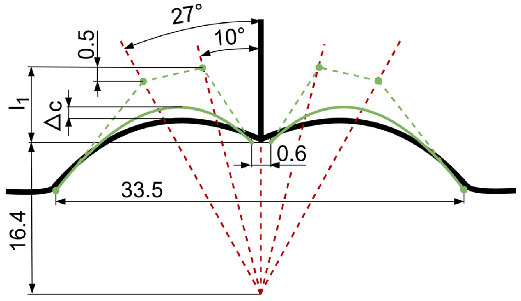
3.7. Bucket Base, Depth

In another four steps, the bucket base defects described in Section 3.6 were further processed, increasing the depth g_d from 0.25 mm to 1.25 mm.

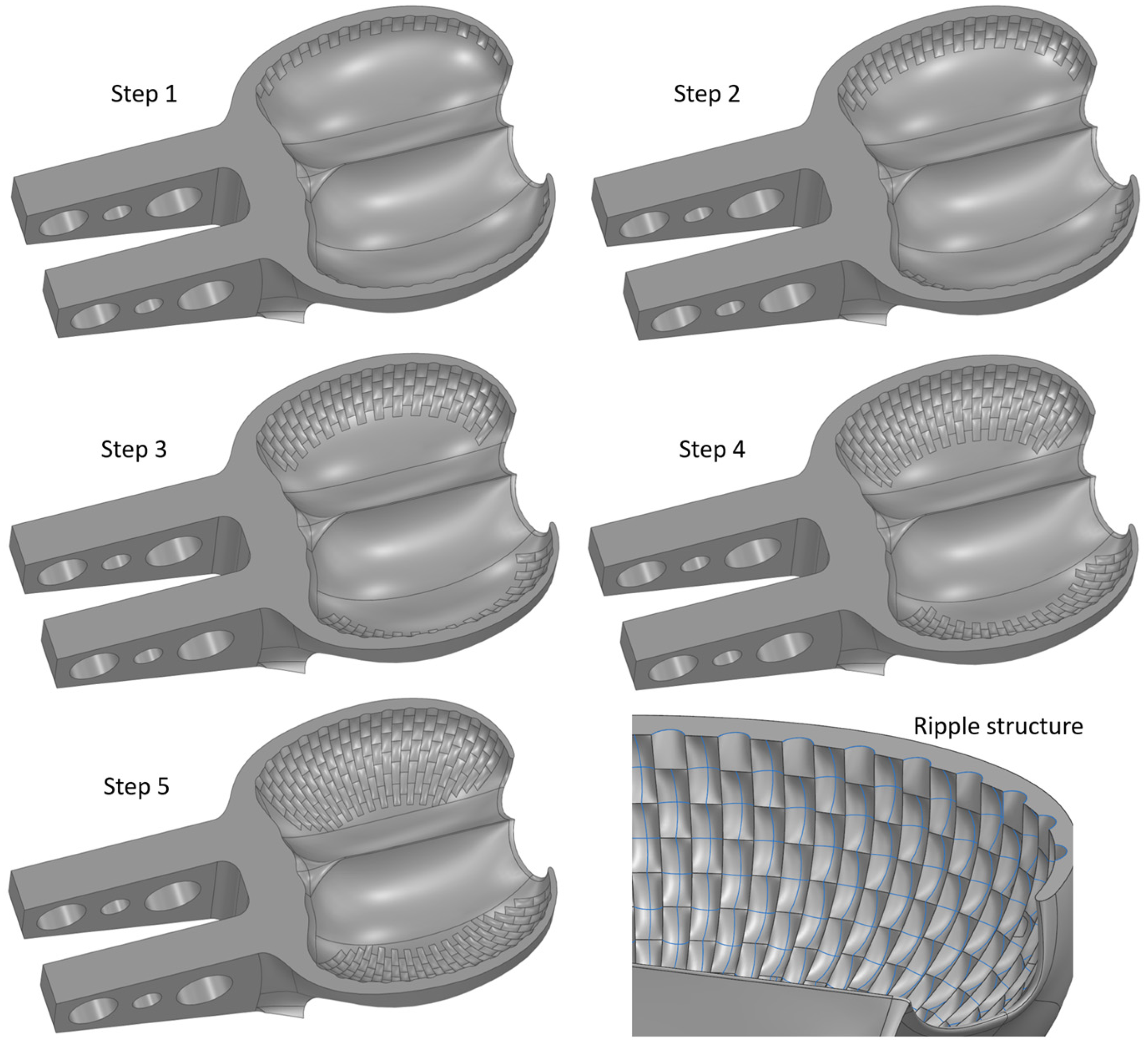
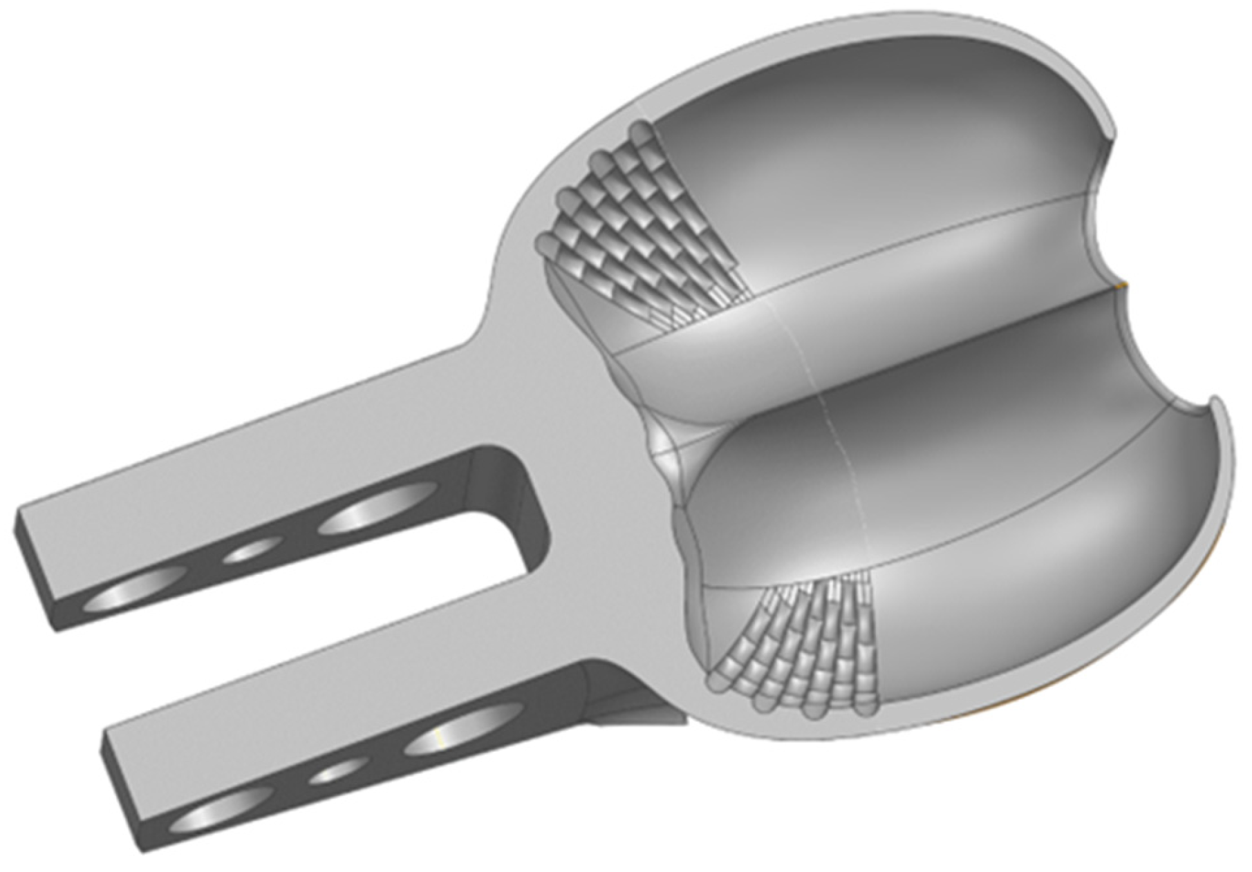
3.8. Bucket Sides, Number of Ripples

The scaly erosion patterns observed on the inside of the buckets, mostly of uncoated runners, were simulated by machining an increasing number of ripples on the surface (see Figure 13). Five steps with increasing rows of ripples were tested. The depth bd of all ripples in these test series was 0.4 mm. The ripple sizes were kept constant in their height (b_r = 6 mm) and width (b_a = 2 mm at the bottom row to 3 mm at the top row).

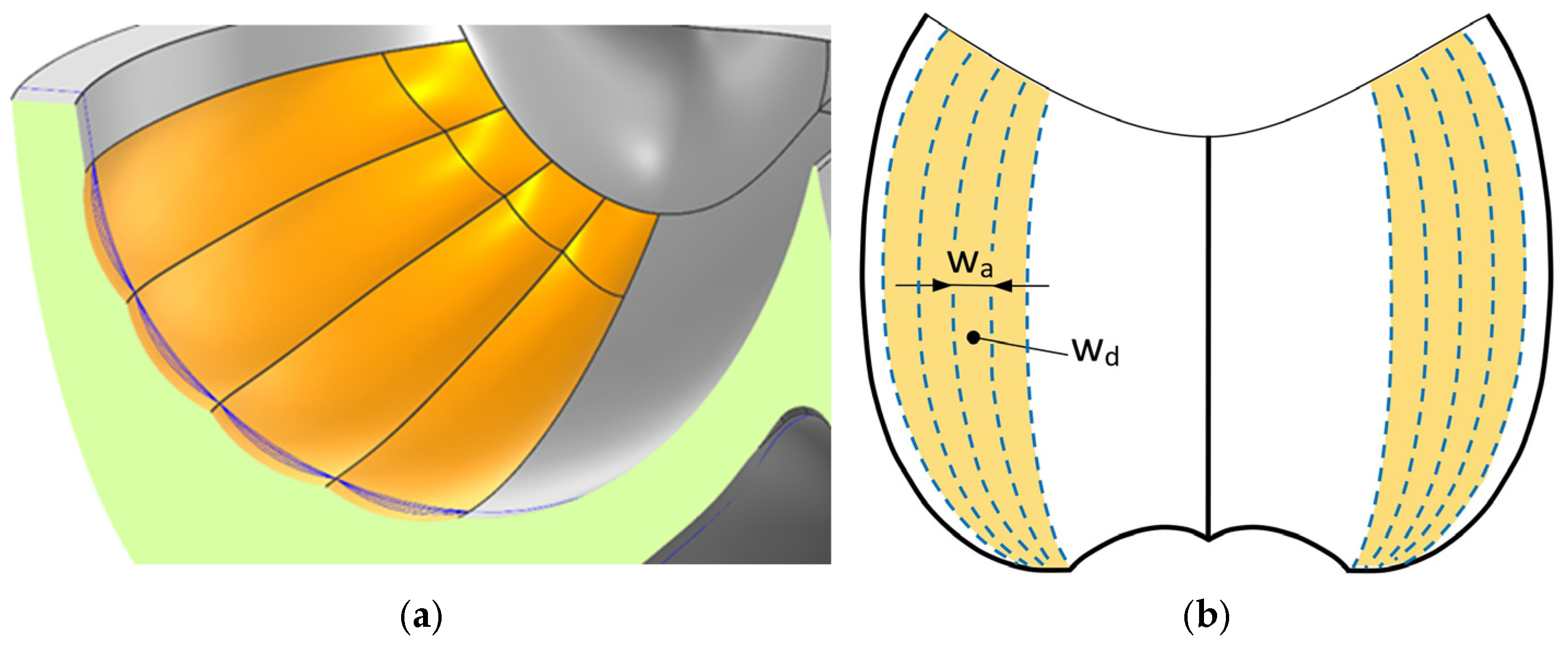
3.9. Bucket Sides, Depth of Ripples

In a further three steps, the depth of the ripples described in Section 3.8 was increased from 0.4 mm to 1.3 mm with steps of 0.3 mm. The size of the structures was kept constant.

3.10. Bucket Side in Bucket Root

The erosion observed on the root on the inside of coated buckets was determined with the same ripples as described in Section 3.8, but just a third of the surface was machined (Figure 14). These test series were performed with runner 8. In three steps, the depth of the ripples was increased from 0.4 mm to 1.3 mm with steps of 0.3 mm. The size of the structures was kept constant.

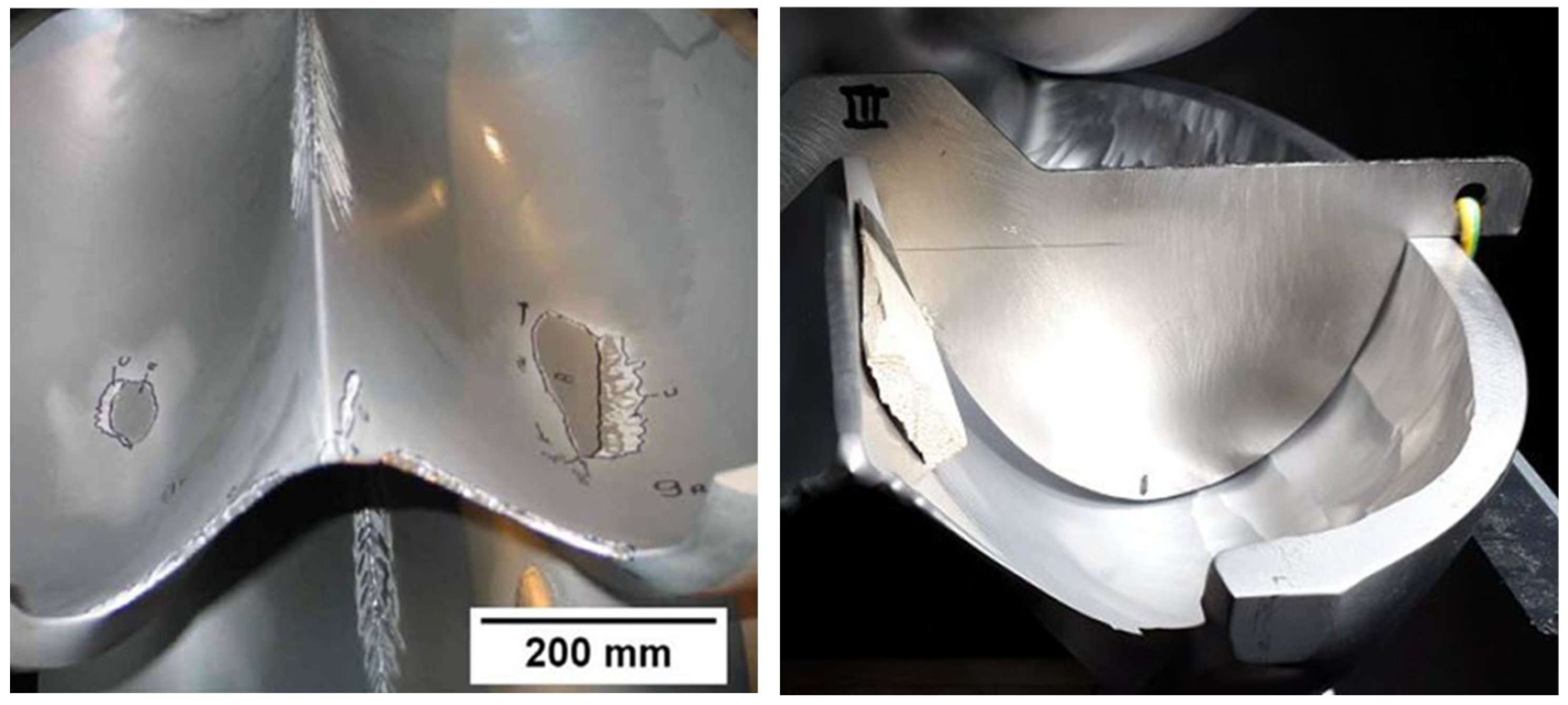
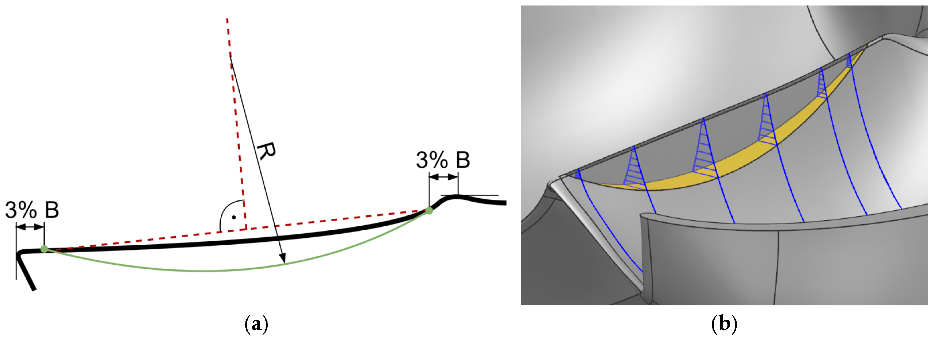
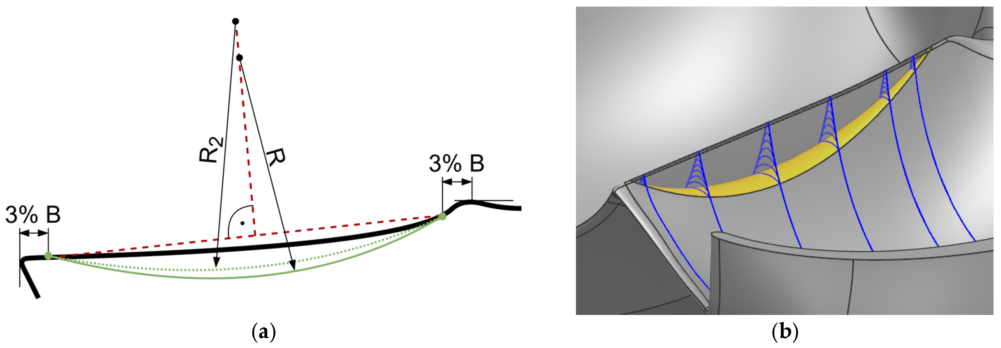
3.11. Wave-Type Defects at Bucket Wall

In addition to the ripple structures on the bucket walls, the effect of wave-like structures along the walls was investigated with runner 9. Four such waves with a width of w_a = 7.35 mm were machined. The depth w_d was increased in 5 steps which were 0.1, 0.2, 0.35, 0.55, and 0.80 mm. The dimensions and machining steps are shown in Figure 15.

3.12. Superposition of Defects

In addition to the defects described above, a series of tests were conducted in which different types of defects were superimposed. For this, different modifications were applied to the same runner one after the other. The processing steps and the number of hill chart measurements are listed in

Table 3. Hill chart measurements of 1 reference runner and 8 stepwise machined runners.

Runner No.	Modifications	Section	Series Name	Machining Steps	Number of Measured Hill Charts
1	Unmodified runner for reference measurements		R	1–7	11
2	Sharp-edged splitter	Section 3.1	A	1–7	8
	+Cutout	Section 3.3	B	8–14	7
	+Splitter tip	Section 3.4	C	15–21	7
	+Bucket base indentation, sharp	Section 3.6	U	22–25	4
	+Bucket base indentation depth, sharp	Section 3.7	V	26–29	4
3	Rounded splitter	Section 3.2	D	1–7	8
	+Cutout	Section 3.3	E	8–14	7
	+Splitter tip	Section 3.4	F	15–21	7
4	Cutout	Section 3.3	G	1–7	8
	+Splitter tip	Section 3.4	H	8–14	7
	+Sharp-edged splitter	Section 3.1	S	15–21	7
5	Cutout + Splitter tip	Section 3.5	J	1–7	8
	+Bucket base indentation, smooth	Section 3.6	M	8–11	4
	+Bucket base indentation depth, smooth	Section 3.7	N	12–15	4
	+Rounded splitter	Section 3.2	T	16–22	7
6	Bucket side	Section 3.8	K	1–5	6
	+Bucket side depth	Section 3.9	L	6–7	2
7	Sharp-edged splitter + Cutout + Splitter tip	Section 3.1, Section 3.3, Section 3.4	P	1–7	8
8	Bucket side in bucket root	Section 3.10	Q	1–3	4
9	Waveform defects at bucket walls	Section 3.11	X	1–5	6

.

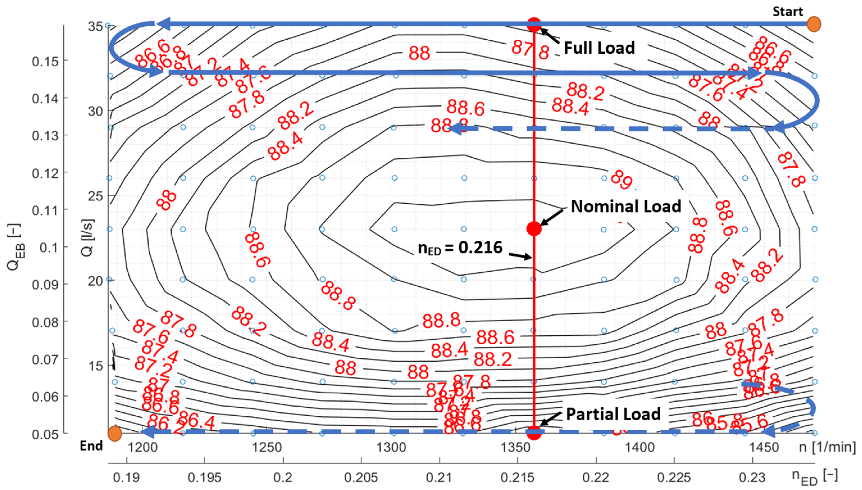
4. Hill Chart Measurement

4.1. Procedure

The hill chart shows the curves of the constant values of turbine efficiency as a function of operating parameters. For each of the steps listed in Table 3, the complete hill chart was measured, for a total of 123 charts. The head was kept constant at 120 m within a range of ±0.1 m. During the tests, the flow rate was varied by operating the nozzle, as well as the rotational speed by varying the load on the generator. For each hill chart, 99 points were measured. The example of the hill chart measurement with runner 1 dated 9 May 2022 is depicted in Figure 16. The blue dots indicate each of these 99 measuring points. The iso-efficiency curves were determined from two-dimensional, linear interpolation of the measured data. The series of measurements always followed the same sequence, starting with high flow rates and gradually increasing or decreasing the speed from 1187 to 1470 rpm in each row with a constant flow rate.

For non-dimensional representation (second axis label in Figure 16) and further analysis of the hill charts, the discharge factor and the speed factor defined in [28], Annex A, were used.

Discharge factor

$$Q_{EB}={\displaystyle \frac{Q}{{B^{2}E}^{0.5}}}$$

(20)

Speed factor

$$n_{ED}={\displaystyle \frac{nD}{E^{0.5}}}$$

(21)

The line at n_ED = 0.216 is highlighted in Figure 16. In the subsequent evaluation of efficiency drops with increasing defects, this line is selected for the presentation of detailed results. Since efficiency drops are significantly more dependent on the discharge factor than on the speed factor, selected results are presented on this highlighted line. Turbines in hydropower plants are commonly operated at or near this speed factor, which is close to the best efficiency.

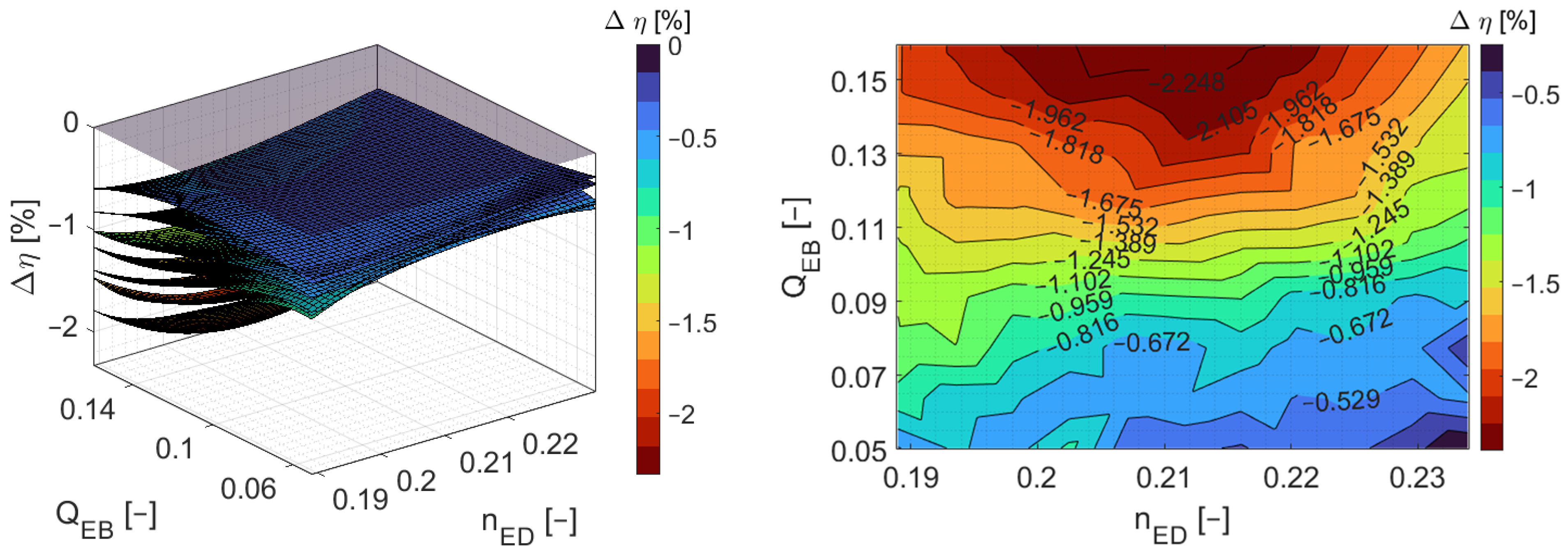
4.2. Example of Sharp-Edged Splitter (Series A, Section 3.1)

Sharp-edge splitter tests are presented in the following example. In each machining step, the splitter width in the mid position was increased by 0.5 mm. The maximum width of 3.5 mm was reached in step 7, corresponding to 4.375% of the inner bucket width.

The hill chart was measured after each machining step. The observed efficiency drop increased almost linearly at each of the 99 measured points. On the left side of Figure 17, the efficiency drops at each of the points are interpolated by a third-degree polynomial. On the right side, the efficiency drop between step 0 and 7 is represented by iso-lines of efficiency loss. At the best efficiency point of the hill chart, this loss is approximately 1.5% (efficiency points with respect to the original efficiency).

Although the graph on the left side of Figure 17 does not provide direct quantitative data for correlation of efficiency loss from step to step, it does give an overview of the deformation of the hill charts with increasing splitter crest machining. For the selected example with a sharp-edged splitter, we see a much larger drop in efficiency at low flow rates, that is, at a low discharge factor. At the upper bound, with high flow rates, Figure 17 right, the drop between step 0 and 7 is about 0.8%, while at the lower bound, with low flow rates, it amounts to 2.3%. When the speed factor is varied, however, there is no clear trend. Within the uncertainty of the measurement, the drop in efficiency seems to be independent of the speed factor.

The drop in efficiency at low flow rates can be physically explained by the increasing ratio of splitter width to jet diameter. As this ratio increases, its influence on the local losses of the impinging jet increases.

4.3. Example of the Cutout (Series G, Section 3.3)

The example of the tests with the increased cutout depth shows opposite effects on efficiency compared to the splitter machining. The maximum cutout depth, in the center of each cutout, has also increased in each step by 0.5 mm, reaching 3.5 mm at step 7.

The graph on the right side of Figure 18 shows a smaller drop in efficiency at low discharge factors (up to 0.5%), increasing to about 2.2% at full load. While the dependence of the drop on the discharge factor is strong, it is less pronounced for the speed factor.

The physical explanation for the opposite trend can again be found in the jet diameter, but this time the negative effect of the increased cutout depth is worse for large jet diameters, as the incidence angle of the jet is degraded over a larger range.

4.4. Examples of Waveform Defects at Bucket Walls (Series X, Section 3.11)

Wavelike defects are typically observed in uncoated buckets exposed to hydro-abrasive erosion. Five machine steps with an increasing depth of the waves were applied. As can be seen in Figure 19, left, the first three machining steps are responsible for only a minor drop in efficiency, while after that the decay increases rapidly. While there is practically no influence of the speed factor, the influence of the discharge factor decreases over-proportionally for low flow rates.

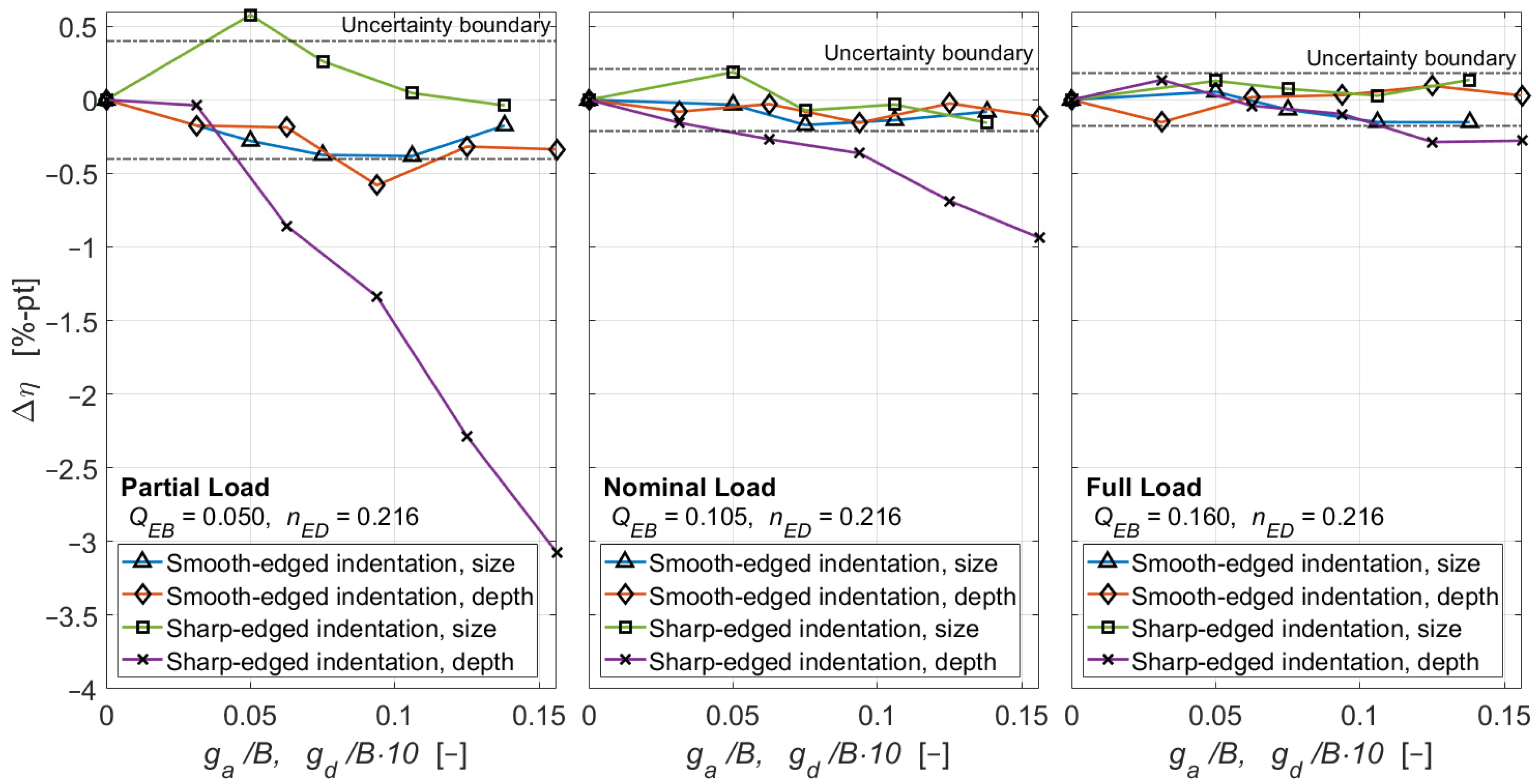
4.5. Efficiency Decay Due to Indentations in the Bucket Base (Series M, N, U, and V, Section 3.6 and Section 3.7)

The defects in the bucket base include indentations of variable size and depth. The effect of smooth-edged indentations of varying sizes was measured in series M and with an increasing depth in series N. The effect of sharp-edged indentations of varying sizes was measured in series U and with an increasing depth in series V. Three points in the hill chart were selected for presentation at speed factor n_ED = 0.216. The three different flow rates correspond to partial load (Figure 20, left), nominal load (Figure 20, center), and full load (Figure 20, right). With the exception of the series V measurements, no clear trends for the efficiency drops could be identified. Most of the variations of the measuring points lie within the uncertainty band. At partial load, the losses of series V increase over-proportionally with the decrease of the flow rate.

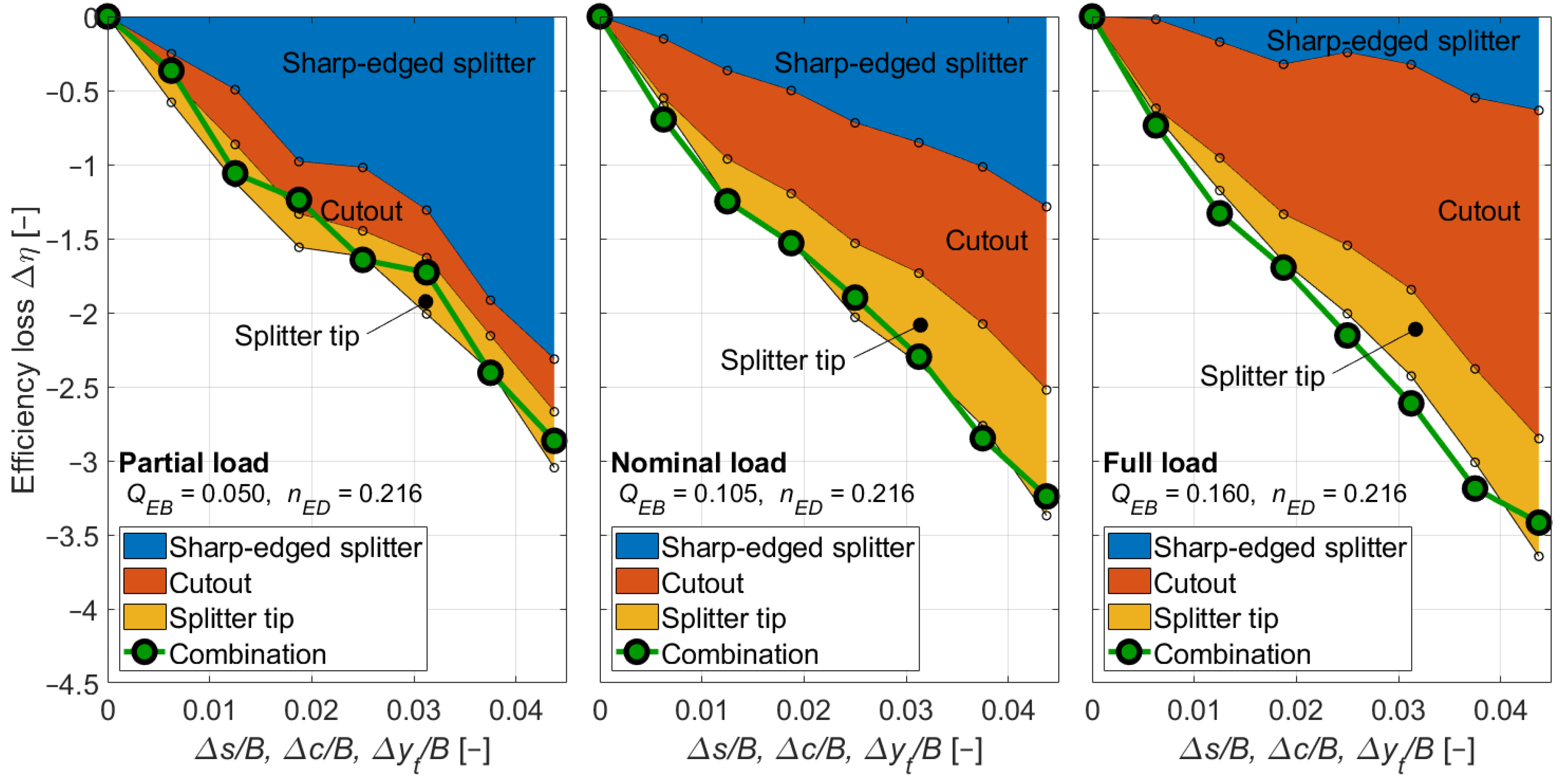
4.6. Combination of Splitter, Cutout, and Tip (Series P)

In the series P measurements, the combination of the simultaneous machining of splitter (sharp-edged), cutout, and tip was carried out in 7 steps. The results of these measurements are connected by green lines in Figure 21. Three points in the hill chart were selected for presentation at speed factor n_ED = 0.216. The three different flow rates correspond to partial load (left), nominal load (center), and full load (right). The summed up individual efficiency drops of series A, G, and H lead to the same results as the ones of the combined measurements, series P. The conclusion from this finding is that the individual efficiency drops can be superimposed. Obviously, the splitter dominates the losses at partial load, while those due to the cutout dominate at full load.

4.7. Types of Efficiency Decay

Two fundamentally different types of efficiency decay were identified. In the case of one type of damage, a linear drop in efficiency was detected from the very beginning (Figure 22, left); in the case of the other, this linear drop began after a threshold value was reached, Figure 22, right.

Above a certain threshold, the decay in efficiency becomes close to linear with the defect depth for all machined defects (splitter, cutout, tip, bucket base, and all types of machined bucket walls). A threshold value was observed for the waveform defects at the bucket walls. There was no threshold value for the splitter, the cutout, and the tip.

5. Conclusions

A strategy was developed for the systematic investigation of typical damages found in Pelton turbines. For this investigation, nine identical runners were fabricated. Individual hill chart measurements of these runners showed a reproducibility of the average efficiency in the range of about 0.15%. One runner was kept in its original state throughout the entire project, while the other eight runners were machined to increase the size, depth, or number of the defects. Due to the different nature of the individual defects, the idea behind the procedure was the assumption that the efficiency deficits of each local damage can be superimposed.

The tests performed and the associated hill charts covered a typical operational range of Pelton turbines in hydropower plants. Since uncertainty and reproducibility are of paramount importance for such a planned test series, a careful uncertainty analysis was performed, as well as a test series to verify the reproducibility over the entire test period.

To illustrate the investigation procedure, examples of machining steps and efficiency measurements are shown for selected cases. The evaluated hill charts of the different processed defects show typical characteristics. Common to the majority of cases is that the dependence of the efficiency decay is dominated by the discharge factor Q_EB. The dependence on the speed factor n_ED is less pronounced. With the exception of the cutout, all efficiencies decrease prominently at low discharge factors. In the case of machined defects at the cutout, the efficiency drops more at high discharge factors. The largest efficiency drops, in the order of 10%, were measured for the L series on the bucket sides (Section 3.8 and Section 3.9) after the final machining steps. Maximum efficiency drops in the range of 5 to 10% were found for the X series with wave-type defects on the bucket walls (Section 3.11). The combination of machining the sharp-edged splitter, cutout, and splitter tip (Section 3.1, Section 3.3 and Section 3.4) in series P resulted in a maximum efficiency drop of 3.5%.

The effect of the indentation in the bucket base was surprisingly low, with the exception of the sharp-edged indentation at maximum width and depth. The measured efficiency drop was within the range of the measurement uncertainty.

Probably, the most important finding of this study is that, in general, the efficiency decreases in a good approximation linearly with the depth of machining in the considered range. This linear decrease in efficiency starts for all defects from the beginning of the machining except for the bucket walls, which show a linear decrease after reaching a certain threshold value. In addition, most of the efficiency drops of the individually investigated defects could be superimposed and gave the same results as the combined measurements of the runners with all defects. For plant operators, this means that individual defects can be analyzed separately and the associated efficiency loss can be determined accordingly. The total expected efficiency loss of the turbines is then a summation of the individual losses. This data, combined with measurements of damages in hydropower plants, can be used to predict current efficiency losses.

References

1. Ge, X.; Sun, J.; Chu, D.; Liu, J.; Zhou, Y.; Zhang, L.; Chen, H.; Binama, M.; Zheng, Y. Sediment erosion on Pelton turbines: A review. Chin. J. Mech. Eng. 2023, 36, 64. [Google Scholar] [CrossRef]
2. Shrivastava, N.; Rai, A.K. Hydro-abrasive erosion in Pelton turbines: Comprehensive review and future outlook. Renew. Sustain. Energy Rev. 2025, 207, 114957. [Google Scholar] [CrossRef]
3. Rai, A.K. Hydro-Abrasive Erosion of Pelton Turbine. Ph.D. Thesis, IIT Roorkee, Roorkee, India, 2017. [Google Scholar]
4. Abgottspon, A.; Staubli, T.; Bieri, E.; Felix, D. Economic optimization of maintenance measures based on continuous efficiency monitoring. In Proceedings of the Vienna Hydro 2022, Vienna, Austria, 9–11 November 2022. [Google Scholar]
5. Rai, A.K.; Kumar, A.; Staubli, T. Financial analysis for optimization of hydropower plants regarding hydro-abrasive erosion: A study from Indian Himalaya. In Proceedings of the 29th Symposium of Hydraulic Machinery and Systems, Kyoto, Japan, 17–21 September 2018. [Google Scholar]
6. Martinez-Monseco, F.J. Analysis of maintenance optimization in a hydroelectric power plant. J. Appl. Res. Technol. Eng. 2020, 1, 23–29. [Google Scholar] [CrossRef]
7. International Bank for Reconstruction and Development/The World Bank. Operation and Maintenance Strategies for Hydropower, Handbook for Practitioners and Decision Makers; The World Bank: Washington, DC, USA, 2020. [Google Scholar]
8. Felix, D. Experimental Investigation on Suspended Sediment, Hydro-Abrasive Erosion and Efficiency Reductions of Coated Pelton Turbines. Ph.D. Thesis, ETHZ, Zürich, Switzerland, 2017. [Google Scholar]
9. Thapa, B. Sand Erosion in Hydraulic Machinery. Ph.D. Thesis, Faculty of Engineering & Technology, NTNU, Trondheim, Norway, 2004. [Google Scholar]
10. Bajracharya, T.R.; Acharya, B.; Joshi, C.B.; Saini, R.P.; Dahlhaug, O.G. Sand erosion of Pelton turbine nozzles and buckets: A case study of Chilime Hydropower Plant. Wear 2008, 26, 177–184. [Google Scholar] [CrossRef]
11. Padhy, M.K.; Saini, R.P. Study of silt erosion on performance of a Pelton turbine. Energy 2011, 36, 141–147. [Google Scholar] [CrossRef]
12. Padhy, M.K.; Saini, R.P. Effect of size and concentration of silt particles on erosion of Pelton turbine buckets. Energy 2009, 34, 1477–1483. [Google Scholar] [CrossRef]
13. Felix, D.; Kastinger, M.; Cracknell, N.; Boes, R. Umgang mit Feinsedimenten am Kleinwasserkraftwerk Susasca; Fachtagung Kleinwasserkraft: Flums, Switzerland, 2023. [Google Scholar]
14. Abgottspon, A.; Staubli, T.; Felix, D. Erosion of Pelton buckets and changes in turbine efficiency measured in the HPP Fieschertal. In Proceedings of the 28th IAHR Symposium on Hydraulic Machinery and Systems, Grenoble, France, 4–8 July 2016; Volume 48, p. 122008. [Google Scholar]
15. Felix, D.; Kastinger, M.; Cracknell, N.; Davidis, S.; Marschall, Y.; Albayrak, I.; Boes, R. OptiSed—Optimierung von Hochdruck-Kleinwasser-Kraftanlagen an feinsedimentreichen Flüssen. In Fallstudie zu Entsandung und Turbinenabrasion am Kleinwasserkraftwerk Susasca; SI/501760; Swiss Federal Office of Energy (SFOE) Bundesamt für Energie: Bern, Switzerland, 2023. Available online: https://www.aramis.admin.ch/Texte/?ProjectID=41589 (accessed on 5 February 2025).
16. Khan, R.; Ullah, S.; Qahtani, F.; Pao, W.; Talha, T. Experimental and numerical investigation of hydro-abrasive erosion in the Pelton turbine buckets for multiphase flow. Renew. Energy 2024, 222, 119829. [Google Scholar] [CrossRef]
17. Rai, A.K.; Kumar, A.; Staubli, T. Hydro-abrasive erosion in Pelton buckets: Classification and field study. Wear 2017, 392–393, 8–20. [Google Scholar] [CrossRef]
18. Abgottspon, A.; von Burg, M.; Staubli, T.; Felix, D. Analysis of hydro-abrasive erosion and efficiency changes measured on the coated Pelton turbines of HPP Fieschertal. In Proceedings of the 30th IAHR Symposium on Hydraulic Machinery and Systems, Lausanne, Switzerland, 5–10 July 2021; Volume 774, p. 012030. [Google Scholar]
19. Brekke, H.; Wu, Y.L.; Cai, B.Y. Design of Hydraulic Machinery Working in Sand Laden Water. In Abrasive Erosion & Corrosion of Hydraulic Machinery; Duan, C.G., Karelin, V.Y., Eds.; Imperial College Press: London, UK, 2002; pp. 155–233. [Google Scholar]
20. Bozic, H.; Hassler, P.; Schnablegger, W. Prüfung und Bewertung von Peltonlaufrädern—Unter besonderer Bedachtnahme auf den Trend zu geschmiedeten Laufrädern. In Proceedings of the Jahrestagung der Deutschen, Österreichischen und Schweizerischen Gesellschaft für Zerstörungsfreie Prüfung, Salzburg, Austria, 17–19 May 2004; DGZfP: Berlin, Germany, 2004. [Google Scholar]
21. Maldet, R. Pelton runner with high erosion caused by glacier sediment: Assessment and measures. In Proceedings of the 15th International Seminar on Hydropower, Vienna, Austria, 26–28 November 2008; pp. 639–646. [Google Scholar]
22. Zhang, Z. Pelton Turbines; Springer: Berlin/Heidelberg, Germany; New York, NY, USA, 2016. [Google Scholar]
23. Liu, J.; Liu, X.; Chang, X.; Qin, B.; Pang, J.; Lai, Z.; Jiang, D.; Qin, M.; Yao, B.; Zeng, Y. Research on the mechanism of sediment erosion in the bucket of a large-scale Pelton turbine at a hydropower station. Powder Technol. 2025, 455, 120805. [Google Scholar] [CrossRef]
24. Guo, B.; Xiao, Y.X.; Rai, A.K.; Liang, Q.W.; Liu, J. Analysis of the airwater-sediment flow behavior in Pelton buckets using a Eulerian-Lagrangian approach. Energy 2021, 218, 119522. [Google Scholar] [CrossRef]
25. Guo, B.; Xiao, Y.X.; Rai, A.K.; Zhang, J.; Liang, Q.W. Sediment-laden flow and erosion modeling in a Pelton turbine injector. Renew. Energy 2020, 162, 30–42. [Google Scholar] [CrossRef]
26. Shrivastava, N.; Rai, A.K. Numerical analysis of hydro-abrasive erosion in a five-jet Pelton turbine distributor. Flow Meas. Instrum. 2025, 103, 102855. [Google Scholar] [CrossRef]
27. ISO 4185:1980; Measurement of Liquid Flow in Closed Conduits, Weighing Method. ISO: Geneva, Switzerland, 1980.
28. IEC 63461:2024; Pelton Hydraulic Turbines—Model Acceptance Tests. IEC: Geneva, Switzerland, 2024.
Figure 1. Schematic representation of the test rig including instrumentation.
Energies 18 02716 g001
Figure 2. Torque measurements on the swinging arms of the generator (left) and the bearing block (right).
Energies 18 02716 g002
Figure 3. Results of reproducibility measurements of 9 identical runners.
Energies 18 02716 g003
Figure 4. Types of erosion with respective location in a Pelton bucket reproduced from [17]. (a): bucket surfaces, (b): bucket backside and (c): splitter.
Energies 18 02716 g004
Figure 5. Examples of defects in the base of a coated bucket in HPP Baspa II in India [3] (left) and of typical waviness of the surface of uncoated buckets, Susasca [15] (right).
Energies 18 02716 g005
Figure 6. Increasing the splitter width with sharp edges. (a): geometrical parameters, (b): machining steps.
Energies 18 02716 g006
Figure 7. Increasing the splitter width with rounded edges. (a): geometrical parameters, (b): machining steps.
Energies 18 02716 g007
Figure 8. The definition of the geometry for the machining of the cutout (top) and a comparison of all 7 machining steps (top view in the (middle), 3D view at the (bottom)).
Energies 18 02716 g008aEnergies 18 02716 g008b
Figure 9. The definition of the geometry for the machining of the tip removal (top) and a comparison of all 7 machining steps (bottom).
Energies 18 02716 g009
Figure 10. The definition of the geometry for the simultaneous machining of the tip and cutout removal (top) and a comparison of all 7 machining steps (top view in the middle, 3D view at the bottom).
Energies 18 02716 g010
Figure 11. The definition for machining the bucket base (left) and a comparison of all 4 machining steps (right).
Energies 18 02716 g011
Figure 12. Geometrical difference between machining of bucket base (left) and bucket base sharp (right).
Energies 18 02716 g012
Figure 13. The definition for machining the inner bucket sides with an increasing number of ripples.
Energies 18 02716 g013
Figure 14. The definition for machining the inner bucket sides in the root with an increasing depth of a defined number of ripples.
Energies 18 02716 g014
Figure 15. The definition for machining waveform defects at the bucket walls (b) and machining steps (a).
Energies 18 02716 g015
Figure 16. The procedure for measuring the hill chart of efficiency.
Energies 18 02716 g016
Figure 17. The efficiency decay for the seven machining steps of the sharp-edged splitter (left) and hill chart of the efficiency drop between reference (step 0) and step 7 (right).
Energies 18 02716 g017
Figure 18. The efficiency decay for the seven machining steps of the cutout (left) and the hill chart of the efficiency drop between reference (step 0) and step 7 (right).
Energies 18 02716 g018
Figure 19. The efficiency decay for the five machining steps of the waveform defects at bucket walls (left) and the hill chart of the efficiency drop between reference (step 0) and step 5 (right).
Energies 18 02716 g019
Figure 20. Example of efficiency drop due to indentations in bucket base (nED = 0.216, QEB = 0.050 (left), QEB = 0.105 (center), QEB = 0.160 (right)): measurement series M, N, U, and V.
Energies 18 02716 g020
Figure 21. Superposition of efficiency drops of splitter, cutout, and tip: 7 steps of individual defects and 7 steps for the combination at nED = 0.216, QEB = 0.050 (left), QEB = 0.105 (center), QEB = 0.160 (right).
Energies 18 02716 g021
Figure 22. Evaluation of slope of efficiency decay in operating point 74 (nED = 0.203, QEB = 0.0775). Sharp-edged splitter, series A (left). Waveform defects at bucket walls, series X (right).
Energies 18 02716 g022