Enhancing Pumped Hydro Storage Regulation Through Adaptive Initial Reservoir Capacity in Multistage Stochastic Coordinated Planning

Abstract

Hybrid pumped hydro storage plants, by integrating pump stations between cascade hydropower stations, have overcome the challenges associated with site selection and construction of pure pumped hydro storage systems, thereby becoming the optimal large-scale energy storage solution for enhancing the absorption of renewable energy. However, the multi-energy conversion between pump stations, hydropower, wind power, and photovoltaic plants poses challenges to both their planning schemes and operational performance. This study proposes a multistage stochastic coordinated planning model for cascade hydropower-wind-solar-thermal-pumped hydro storage (CHWS-PHS) systems. First, a Hybrid Pumped Hydro Storage Adaptive Initial Reservoir Capacity (HPHS-AIRC) strategy is developed to enhance the system’s regulation capability by optimizing initial reservoir levels that are synchronized with renewable generation patterns. Then, Non-anticipativity Constraints (NACs) are incorporated into this model to ensure the dynamic adaptation of investment decisions under multi-timescale uncertainties, including inter-annual natural water inflow (NWI) variations and hourly fluctuations in wind and solar power. Simulation results on the IEEE 118-bus system show that the proposed MSSP model reduces total costs by 6% compared with the traditional two-stage approach (TSSP). Moreover, the HPHS-AIRC strategy improves pumped hydro utilization by 33.8%, particularly benefiting scenarios with drought conditions or operational constraints.

1. Introduction

To address the global energy crisis and climate change challenges, future power system planning is transitioning towards a clean, low-carbon energy structure dominated by renewable energy (RE), primarily wind and solar photovoltaic (PV) sources [1,2,3,4]. However, the inherent volatility, randomness, and intermittency of RE sources pose significant challenges to the supply–demand balance and operational stability of power systems when integrated at large scales [5,6]. In this context, to ensure reliable electricity supply in power systems with high RE penetration, future power system planning must incorporate advanced energy storage technologies in order to enhance regulatory capacity and stabilize operations [7,8].

Among various energy storage technologies, pumped hydro storage (PHS) has emerged as the most widely utilized large-scale storage solution globally, owing to its high capacity, long lifespan, and efficient energy conversion [9,10]. Nevertheless, traditional PHS typically faces strict topographical and water resource requirements, thus limiting site selection. As a result, hybrid pumped hydro storage (HPHS) has emerged as a promising alternative by retrofitting existing cascade hydropower reservoirs to integrate conventional hydropower with pumped storage units, thereby reducing the need for new reservoir construction and leveraging existing water infrastructure [11,12,13]. Therefore, exploring the coordinated planning of HPHS-wind-solar system has become essential.

Most of the current research on HPHS-wind-solar system focuses on capacity configuration [14,15] and economic evaluation [16,17,18], analyzing the ability to compensate for RE output under different scenarios or capacities. For instance, Zhang et al. [14] investigated the interplay among capacity configuration, electricity prices, and transmission constraints, and proposed three screening principles to reveal the techno–economic interactions. Ak et al. [18] investigated the operational economic benefits of cascade hydropower and HPHS under various natural inflow and electricity price scenarios, and found that HPHS proved to be optimal across different conditions. However, to overcome the computational challenges posed by nonlinearity, the solution was simplified by fixing the variable for environmental flows. In day-ahead scheduling, Mengke Lu et al. [19] utilized an optimization model to effectively reduce the start–stop frequency and output fluctuations of thermal power units. In terms of economic evaluation, Zhang et al. [20] found that HPHS can effectively reduce wind and solar curtailment and that different pumping efficiencies have an impact on economic performance. Although these studies analyze the effectiveness of HPHS in compensating for wind and solar output from different perspectives, a knowledge gap still exists in the literature regarding the coordinated planning of HPHS-wind-solar systems.

In the coordinated planning of such hybrid systems, it is necessary not only to consider the operational schedule within each dispatch cycle but also to determine the investment strategies for HPHS, wind turbines, and PV plants under different scenarios. Our simulation experiments reveal that if the modeling approach for HPHS from [21]—which treats the initial reservoir capacity (IRC) in each dispatch stage as a fixed value—is continued, the IRC will not be flexibly adjusted to reflect fluctuations in wind and solar output. This inflexibility leads to premature depletion of water resources during the pumping period, preventing the full utilization of the regulatory capability of HPHS. Moreover, the approach in [16] that ignores IRC constraints, while ensuring adequate water resources, results in physically infeasible outcomes due to the lack of proper IRC constraint. More seriously, an unreasonable reservoir capacity configuration can even affect the investment planning for pumped storage units. Therefore, it is necessary to propose a scheduling strategy for IRC that allows for flexible adjustment.

Additionally, the variability in wind and solar output, as well as natural water inflows (NWIs), poses significant operational risks to the system. To address these uncertainties, scenario-based stochastic optimization has become the predominant methodology, with the two-stage stochastic programming (TSSP) model being particularly noteworthy [22,23,24]. However, TSSP cannot dynamically adjust decisions as uncertain information gradually unfolds, leading to suboptimal adaptability in later-stage investments [25]. To overcome this limitation, Multistage Stochastic Programming (MSSP) has garnered attention as a more flexible modeling approach, with Non-anticipativity Constraints (NACs) being one of its core concepts. This ensures that decisions made in the current stage are based solely on known information, without reliance on future information, thereby aligning more closely with the sequential decision-making processes in real-world planning. As a representative application, Ding et al. [25] proposed a NAC-based MSSP model to coordinate the expansion planning of power and electricity systems while accounting for the uncertainty in net load demand. Zhang et al. [26] developed a mobile emergency generator planning model incorporating NACs in order to optimize post-disaster recovery strategies, while Cobos et al. [27] further introduced a multistage robust unit commitment model that specifically addresses the non-anticipatory nature of wind power uncertainty. As the uncertainties associated with wind, solar, and NWIs evolve over distinct timescales [28,29,30], it is essential to classify and model them appropriately to accurately capture their impacts on system planning and operation.

Based on the above analysis, this study proposes a coordinated planning approach for a cascade hydropower-wind-solar-thermal-pumped hydro storage (CHWS-PHS) system, aiming to comprehensively consider investment decisions related to transmission expansion and the retirement of thermal power units during the long-term planning stage. Additionally, a novel HPHS-Adaptive Initial Reservoir Capacity (HPHS-AIRC) strategy is introduced in the operational stage to improve the absorption capacity of wind and solar fluctuations and enhance system operational flexibility. To better address uncertainties across different timescales, this paper incorporates NACs within an MSSP framework, facilitating hierarchical modeling and dynamic decision-making processes for inter-annual inflow variations and hourly wind and solar fluctuations. The primary contributions of this paper include:

(1)

Coordinated Planning Model based on MSSP: We develop an MSSP model that dynamically adjusts investment and operational strategies for the CHWS-PHS system, effectively addressing uncertainties and temporal variations in RE output and NWIs. The model incorporates NACs, enabling dynamic adjustments in response to unfolding uncertainties.

(2)

Proposed HPHS-AIRC Strategy: To address the unique reservoir management challenges associated with switching between pumping and generating modes in HPHS, the HPHS-AIRC strategy is proposed. This strategy is integrated into the multistage optimization model to maximize the regulatory potential of HPHS under uncertainties in NWIs and RE generation.

The remainder of this paper is organized as follows: Section 2 presents the coordinated planning model and the proposed HPHS-AIRC strategy; Section 3 discusses the modeling and handling of uncertainties in renewable generation and NWIs; Section 4 provides numerical studies; Section 5 provides discussion; and Section 6 concludes the paper.

2. Coordinated Planning Model

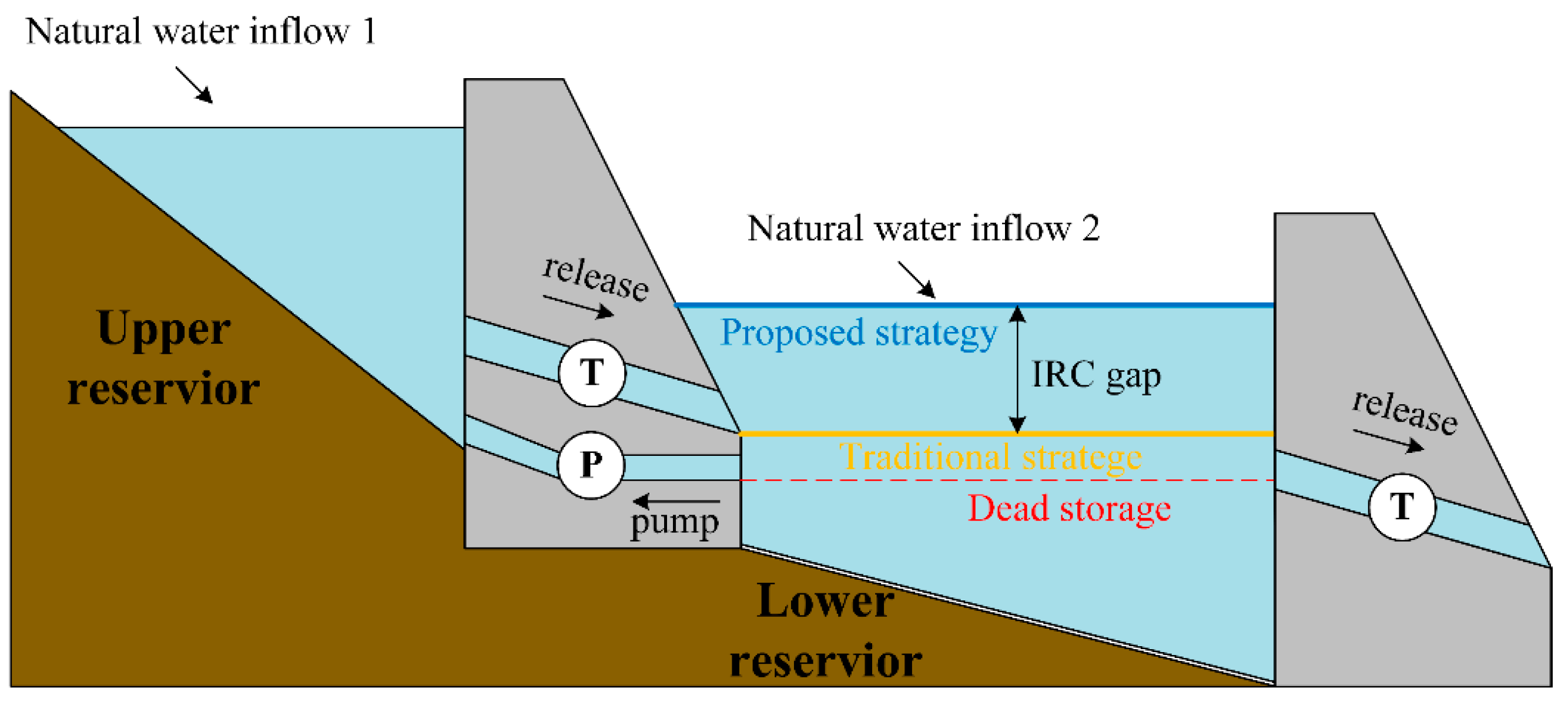
2.1. Proposed HPHS-AIRC Strategy

In the traditional scheduling strategy of cascade hydroelectric stations, the reservoir capacity must meet the capacity limit requirements (as shown in Equation (1)) to ensure safe system operation. Generally, the terminal volume of the hydro units in the current scheduling period is regarded as the same for the subsequent period. Therefore, the IRC is typically close to the lower capacity limit in order to maximize water resource utilization and improve the economic efficiency of system operations, as illustrated in Figure 1.

$$V_{t,0,h}=\underset{¯}{V_h}$$

(1)

where $V_{t,k,h}$ represents the reservoir volume of unit h at time k in stage t and $\underset{¯}{V_h}$ denotes the min value of reservoir volume of unit h.

As shown in Figure 1a, during periods of high RE output and low load, such as between 0:00 and 4:00 at night, the system typically requires PHS to store surplus wind and solar power. However, due to insufficient IRC, the PHS units are unable to start and perform energy storage, resulting in their regulation capability not being fully utilized, which limits the absorption of wind and solar energy.

To address this issue, this paper proposes an HPHS-AIRC strategy, which dynamically adjusts the IRC level for each scheduling period. Unlike traditional methods that rely on a fixed dead storage level, the proposed strategy optimizes the IRC based on the proportion of wind and solar generation and the operational status of the PHS equipment. By adjusting the IRC, the system can better accommodate fluctuations in wind and solar generation and ensure sufficient reservoir capacity to meet nighttime pumping demands, thereby avoiding RE curtailment.

Specifically, the IRC is determined by Equation (2).

$$V_{t,0,h}=\underset{¯}{V_h}+{\delta }^{\mathrm{pump}}\left({\displaystyle \frac{P_t^{wind}+P_t^{solar}}{D_t}}\right)\left(\overline{V_h}-\underset{¯}{V_h}\right)y_{t,h}^{\mathrm{pump}}$$

(2)

where ${\delta }^{\mathrm{pump}}$ represents the adaptive rate of HPHS-AIRC; $P_t^{wind}$ and $P_t^{solar}$ denote the total power generation at stage t of wind turbines and PV plants, respectively; $D_t$ signifies the total load demand at stage t; $\overline{V_h}$ denotes the max value of reservoir volume of unit h; and $y_{t,h}^{\mathrm{pump}}$ represents the construction and investment status of HPHS unit h in stage t.

As shown in Figure 1b, the proposed strategy significantly increases the IRC, ensuring effective absorption of surplus RE and avoiding the issue of insufficient water for pumping. Additionally, Figure 2 compares the reservoir levels under the traditional and proposed strategies. It is evident from the figure that the proposed strategy significantly increases the IRC of the lower reservoir (referred to as the IRC gap). This improvement is attributed to the adjustment of reserved pumping flow, which enhances the utilization of PHS and effectively overcomes the inefficiencies of the traditional scheduling strategy.

2.2. Objective Function

The objective of the proposed CHWS-PHS model is to minimize the total investment cost $C^{\mathrm{I}}$ and operational cost $C^{\mathrm{O}}$, with the net present value of the objective calculated using Equation (3).

$$\min {\displaystyle \sum _t^{\mathrm{NT}}\frac{1}{{\left(1+{\sigma }_{dr}\right)}^{t-1}}}\left(C^{\mathrm{I}}+C^{\mathrm{O}}\right)$$

(3)

where $\mathrm{NT}$ represents the number of planning stages and ${\sigma }_{dr}$ denotes the discount rate.

(1)

Investment Cost: The investment cost $C^{\mathrm{I}}$ (Equation (4)) comprises four components: variable-speed HPHS (VS-HPHS) units, wind farms, PV power plants, and transmission lines.

$$\begin{array}{c}{C}^{\mathrm{I}}={\displaystyle \sum _{hϵ\mathrm{CH}}{c}_h^{\mathrm{inv}}\left(y_{t,h}^{\mathrm{pump}}-y_{t-1,h}^{\mathrm{pump}}\right)+{\displaystyle \sum _{wϵ\mathrm{CW}}{c}_w^{\mathrm{inv}}\left(y_{t,w}-y_{t-1,w}\right)}}\\ +{\displaystyle \sum _{sϵ\mathrm{CS}}{c}_s^{\mathrm{inv}}\left(y_{t,s}-y_{t-1,s}\right)}+{\displaystyle \sum _{lϵ\mathrm{CL}}{c}_l^{\mathrm{inv}}\left(y_{t,l}-y_{t-1,l}\right)}\end{array}$$

(4)

where $c_h^{\mathrm{inv}}$, $c_w^{\mathrm{inv}}$, $c_s^{\mathrm{inv}}$, and $c_l^{\mathrm{inv}}$ represent the investment cost of VS-HPHS unit, wind farm, PV power plant, and power line, respectively; $y_{t,w}$, $y_{t,s}$, and $y_{t,l}$ denote the construction and investment status of wind farm w, PV power plant s, and power line l in stage t, respectively; and CH, CW, CS, and CL denote the set of candidate VS-HPHS units, wind farms, PV power plants, and power lines, respectively.

(2)

Operation Cost: The operational cost $C^{\mathrm{O}}$ (Equation (5)) includes the operational costs of thermal units $C^{\mathrm{G}}$ (Equation (6)) and the penalty costs for load shedding $C^{\mathrm{L}}$ (Equation (7)) and for wind and solar curtailment $C^{\mathrm{N}}$ (Equation (8)).

$$C^{\mathrm{O}}={\displaystyle \sum _k^{\mathrm{NK}}\left(C^{\mathrm{G}}+C^{\mathrm{L}}+C^{\mathrm{N}}\right)}$$

(5)

$$C^{\mathrm{G}}={\displaystyle \sum _{gϵ\mathrm{NG}\left(\mathrm{t}\right)}{c}_g^{\mathrm{fuel}}{F}_g\left(P_{t,k,g}\right)}$$

(6)

$$C^{\mathrm{L}}={\displaystyle \sum _{cϵ\mathrm{NC}}{c}_{load}^{\mathrm{shed}}{P}_{t,k,c}^{\mathrm{shed}}}$$

(7)

$$C^{\mathrm{N}}={\displaystyle \sum _{wϵ\mathrm{NW}\left(\mathrm{t}\right)}{c}_w^{\mathrm{shed}}\left(P_{t,k,w}^{\mathrm{f}}-P_{t,k,w}\right)}{y}_{t,w}+{\displaystyle \sum _{sϵ\mathrm{NS}\left(\mathrm{t}\right)}{c}_s^{\mathrm{shed}}\left(P_{t,k,s}^{\mathrm{f}}-P_{t,k,s}\right)}{y}_{t,s}$$

(8)

where NK denotes the number of time steps per stage; $\mathrm{NG}\left(t\right)$, $\mathrm{NC}$, $\mathrm{NW}\left(t\right)$, and $\mathrm{NS}\left(t\right)$ represent the number of units of thermal, node, wind farm, and PV power plants in stage t, respectively; $c_g^{\mathrm{fuel}}$ denotes the operational cost of thermal unit g; $F_g\left(\cdot \right)$ represents the heat rate curve of thermal power unit g; $P_{t,k,g}$ denotes the output of thermal unit g at time k in stage t; $c_{load}^{\mathrm{shed}}$ represents the costs of load curtailment; $P_{t,k,c}^{\mathrm{shed}}$ denotes load shedding at node c at time k in stage t; ${\left(\cdot \right)}^f$ denotes forecasted value of a quantity; $P_{t,k,w}$ and $P_{t,k,s}$ represent the output of wind farm w and PV power plant s at time k in stage t, respectively; and $c_w^{\mathrm{shed}}$ and $c_s^{\mathrm{shed}}$ represent the costs of wind and solar curtailment, respectively.

2.3. Constraints

The model is subject to a series of technical and investment constraints:

(1)

Planning decision constraints:

Planning decision constraints include several key aspects to ensure proper investment, operation, and decommissioning of equipment in the system. First, investment in each equipment type occurs only once, as specified in the following constraints (9)~(12).

$$y_{t-1,h}^{\mathrm{pump}}\le y_{t,h}^{\mathrm{pump}}\le 1,\forall hϵ\mathrm{CH}$$

(9)

$$y_{t-1,w}\le y_{t,w}\le 1,\forall wϵ\mathrm{CW}$$

(10)

$$y_{t-1,s}\le y_{t,s}\le 1,\forall sϵ\mathrm{CS}$$

(11)

$$y_{t-1,l}\le y_{t,l}\le 1,\forall lϵ\mathrm{CL}$$

(12)

In addition to investment constraints, decommissioning rules ensure the orderly retirement and commissioning of units. For thermal units, retirement is mandatory once the unit reaches its decommissioning age, as defined in Equation (13). For HPHS units, they can only operate after being commissioned, which is described in Equation (14):

$$I_{t,k,g}^{\mathrm{thermal}}=0,t\ge T_g^{\mathrm{retire}},\forall gϵ\mathrm{EG}$$

(13)

$$I_{t,k,h}^{\mathrm{pump}}\le y_{t,h}^{\mathrm{pump}},\forall hϵ\mathrm{CH}$$

(14)

where $I_{t,k,g}^{\mathrm{thermal}}$ represents the operating status of thermal unit g at time k in stage t; $T_g^{\mathrm{retire}}$ denotes the retirement stage of thermal unit g; $\mathrm{EG}$ denotes the set of existing thermal power units; and $I_{t,k,h}^{\mathrm{pump}}$ represents the pumping mode operating status of unit h at time k in stage t.

Finally, the operational states of the HPHS units are restricted to pumping, generating, or shutdown modes, ensuring no simultaneous pumping and generating. This restriction is enforced by Equation (15).

$$0\le I_{t,k,h}^{\mathrm{pump}}+I_{t,k,h}^{\mathrm{gen}}\le 1,\forall hϵ\mathrm{CH}$$

(15)

where $I_{t,k,h}^{\mathrm{gen}}$ denotes the generation mode operating status of unit h at time k in stage t.

(2)

VS-HPHS unit constraints:

For the VS-HPHS unit, both the upstream and downstream reservoirs receive NWIs, and any spilled water is discarded directly rather than passed downstream. Based on this, the constraints related to the power-generation unit and pumped-storage operations in the cascade hydropower system are outlined as follows.

(a)

Power-generation unit:

To begin with, the water-outflow constraint ensures that the water outflow remains within the generation capacity of the hydropower system, as expressed in Equation (16).

$$\underset{¯}{Q_h^{\mathrm{gen}}}{I}_{t,k,h}^{\mathrm{gen}}\le Q_{t,k,h}^{\mathrm{gen}}\le \overline{Q_h^{\mathrm{gen}}}{I}_{t,k,h}^{\mathrm{gen}}$$

(16)

where $Q_{t,k,h}^{\mathrm{gen}}$ represents the turbine flow of unit h at time k in stage t and $\underset{¯}{Q_h^{\mathrm{gen}}}$ and $\overline{Q_h^{\mathrm{gen}}}$ denote the min and max value of turbine flow of unit h, respectively.

Simultaneously, the reservoir capacity constraint maintains the reservoir’s volume within its upper and lower capacity limits, as shown in Equation (17).

$$\underset{¯}{V_h}\le V_{t,k,h}\le \overline{V_h}$$

(17)

Furthermore, the reservoir volume is balanced through the following relationship in Equation (18).

$$V_{t,k,h}=V_{t,k-1,h}+r_{t,k,h}+Q_{t,k,h-1}^{\mathrm{gen}}-Q_{t,k,h}^{\mathrm{gen}}+Q_{t,k,h}^{\mathrm{pump}}-Q_{t,k,h-1}^{\mathrm{pump}}-Q_{t,k,h}^{\mathrm{surplus}}$$

(18)

where $r_{t,k,h}$ represents the NWIs of unit h at time k in stage t; $Q_{t,k,h}^{\mathrm{pump}}$ denotes the pump flow of unit h at time k in stage t; and $Q_{t,k,h}^{\mathrm{surplus}}$ represents the curtailment water flow of unit h at time k in stage t.

The continuity of reservoir operations between consecutive scheduling periods is ensured by the following relationship, as shown in Equation (19).

$$V_{t-1,\mathrm{NK},h}=V_{t,0,h}$$

(19)

Next, the water-to-power relationship is described by Equation (20).

$$P_{t,k,h}^{\mathrm{gen}}={\eta }_h^{\mathrm{gen}}{Q}_{t,k,h}^{\mathrm{gen}}\left(h_{0,h}+{\alpha }_h{V}_{t,k,h}\right)$$

(20)

where $P_{t,k,h}^{\mathrm{gen}}$ represents the power generation of unit h at time k in stage t; ${\eta }_h^{\mathrm{gen}}$ represents the water-to-power conversion coefficient of the generation mode of the HPHS unit h; and $h_{0,h}$ and ${\alpha }_h$ denote the constant terms of the reservoir of unit h, which are determined by the physical size of the reservoirs [31].

Finally, the power output of the system is further constrained by the power-output constraint, which limits power generation based on the reservoir volume, as described in Equation (21).

$$\underset{¯}{P_h^{\mathrm{gen}}}{I}_{t,k,h}^{\mathrm{gen}}\le P_{t,k,h}^{\mathrm{gen}}\le \overline{P_h^{\mathrm{gen}}}{I}_{t,k,h}^{\mathrm{gen}}$$

(21)

where, $\underset{¯}{P_h^{\mathrm{gen}}}$ and $\overline{P_h^{\mathrm{gen}}}$ represent the min and max value of the generation power of unit h, respectively.

(b)

Pumped-storage unit:

For the constraints of the pumped-storage unit, the water-outflow constraint, power-output constraint, and water-to-power conversion constraint are defined in Equations (22), (23) and (24), respectively.

$$\underset{¯}{Q_h^{\mathrm{pump}}}{I}_{t,k,h}^{\mathrm{pump}}\le Q_{t,k,h}^{\mathrm{pump}}\le \overline{Q_h^{\mathrm{pump}}}{I}_{t,k,h}^{\mathrm{pump}}$$

(22)

$$0\le P_{t,k,h}^{\mathrm{pump}}\le \overline{P_h^{\mathrm{pump}}}{I}_{t,k,h}^{\mathrm{pump}}$$

(23)

$$P_{t,k,h}^{\mathrm{pump}}={\eta }_h^{\mathrm{pump}}{Q}_{t,k,h}^{\mathrm{pump}}\left(h_{0,h}+{\alpha }_h{V}_{t,k,h}\right)$$

(24)

where $Q_{t,k,h}^{\mathrm{pump}}$ denotes the pump flow of unit h at time k in stage t; $\underset{¯}{Q_h^{\mathrm{pump}}}$ and $\overline{Q_h^{\mathrm{pump}}}$ represent the min and max value of the pump flow for unit h, respectively; $\overline{P_h^{\mathrm{pump}}}$ denotes the max value of the pump power of unit h; and ${\eta }_h^{\mathrm{pump}}$ represents the water-to-power conversion coefficient of the pump mode of the HPHS unit h.

(3)

Thermal unit constraints:

Due to the system being primarily powered by RE units, with a relatively low proportion of thermal power units, only capacity limits (25) and ramp up (26) and down (27) limits are considered.

$$\underset{¯}{P_g}\le P_{t,k,g}\le \overline{P_g}$$

(25)

$$P_{t,k,g}-P_{t,k-1,g}\le R^{\mathrm{up}}{I}_{t,k-1,g}^{\mathrm{thermal}}+\underset{¯}{P_g}\left(I_{t,k,g}^{\mathrm{thermal}}\right.-\left.I_{t,k-1,g}^{\mathrm{thermal}}\right)+\overline{P_g}\left(1-I_{t,k,g}^{\mathrm{thermal}}\right)$$

(26)

$$P_{t,k-1,g}-P_{t,k,g}\le R^{\mathrm{down}}{I}_{t,k,g}^{\mathrm{thermal}}+\underset{¯}{P_g}\left(I_{t,k-1,g}^{\mathrm{thermal}}\right.-\left.I_{t,k,g}^{\mathrm{thermal}}\right)+\overline{P_g}\left(1-I_{t,k-1,g}^{\mathrm{thermal}}\right)$$

(27)

where $\underset{¯}{P_g}$ and $\overline{P_g}$ denote the min and max value of power generation by unit g, respectively, and $R^{\mathrm{up}}$ and $R^{\mathrm{down}}$ represent the ramp rate of the thermal power unit, respectively.

(4)

Wind and solar constraints:

The energy for HPHS is sourced from the surplus output of wind and solar power generation, ensuring optimal utilization and minimizing curtailment, as shown in Equation (28).

$$0\le P_{t,k,w}+P_{t,k,s}+P_{t,k,h}^{\mathrm{pump}}\le P_{t,k,w}^{\mathrm{f}}+P_{t,k,s}^{\mathrm{f}}$$

(28)

(5)

Power flow constraints:

Transmission line capacities are governed by Equations (29)~(33). The “big M” method [31] ensures that flow variables are appropriately constrained based on whether a transmission line is installed or not.

$$P{L}_{t,k,l}{X}_l=\left({\theta }_{t,k,s\left(l\right)}-{\theta }_{t,k,r\left(l\right)}\right),lϵ\mathrm{EL}$$

(29)

$$-\overline{P{L}_l}\le P{L}_{t,k,l}\le \overline{P{L}_l},lϵ\mathrm{EL}$$

(30)

$$-\overline{P{L}_l}{y}_{t,l}\le P{L}_{t,k,l}\le \overline{P{L}_l}{y}_{t,l},lϵ\mathrm{CL}$$

(31)

$$-\left(1-y_{t,l}\right)M\le P{L}_{t,k,l}{X}_l-\left({\theta }_{t,k,s\left(l\right)}-{\theta }_{t,k,r\left(l\right)}\right)\le \left(1-y_{t,l}\right)M,lϵ\mathrm{CL}$$

(32)

$$-\overline{{\theta }_c}\le {\theta }_{t,k,c}\le \overline{{\theta }_c}$$

(33)

where $P{L}_{t,k,l}$ represents power flow at line l at time k in stage t; ${\theta }_{t,k,c}$ denotes the bus angle in the power network at node c at time k in stage t; $\underset{¯}{P{L}_l}$ and $\overline{P{L}_l}$ denote the min and max value of power flow for line l, respectively; $s\left(l\right)$ and $r\left(l\right)$ represent the receiving bus and sending bus for line l, respectively; EL denotes the set of existing transmission lines; M denotes a sufficiently large number of typical values used in similar contexts ranging from 10⁴ to 10⁶; X_l represents the reactance of transmission line l; and $\underset{¯}{{\theta }_c}$ and $\overline{{\theta }_c}$ denote the min and max value of bus angle at node c, respectively.

(6)

Power balance constraints:

At each bus and time period, generation and net imports must meet demand, as modeled by Equation (34).

$$\begin{array}{l}{\displaystyle \sum _{g\in \mathrm{NC}}{P}_{t,k,g}}+{\displaystyle \sum _{h\in \mathrm{NC}}{\mathrm{P}}_{\mathrm{t},\mathrm{k},\mathrm{h}}^{\mathrm{gen}}}-{\displaystyle \sum _{h\in \mathrm{NC}}{P}_{t,k,h}^{\mathrm{pump}}}+{\displaystyle \sum _{w\in \mathrm{NC}}{P}_{t,k,w}}+{\displaystyle \sum _{s\in \mathrm{NC}}{P}_{t,k,s}}\\ -{\displaystyle \sum _{s\left(l\right)\in \mathrm{NC}}P{L}_{t,k,s\left(l\right)}}+{\displaystyle \sum _{r\left(l\right)\in \mathrm{NC}}P{L}_{t,k,r\left(l\right)}}+{\displaystyle \sum _{cϵ\mathrm{NC}}{P}_{t,k,c}^{\mathrm{shed}}}=D_{t,k}\end{array}$$

(34)

where $D_{t,k}$ denotes the total demand for the system at time k in stage t.

2.4. General Mathematical Formulation

Combining all costs and constraints, the CHWS-PHS planning problem is formulated as a multi-period MILP model, incorporating both discrete investment variables x_t and continuous operational variables y_t. The discrete variables are temporally coupled by constraint (35), resulting in the following formulation:

$$\begin{array}{l}\underset{\left\{x_t,y_t\right\}}{\min }{\displaystyle \sum _t^{\mathrm{NT}}{f}_t\left(x_t,y_t\right)}\\ s.t. D_t{x}_{t-1}+C_t{x}_t=b_t,t=1,\dots ,NT\\ \hspace{1em}\hspace{1em}\left(x_t,y_t\right)\in {\Psi }_t,t=1,\dots ,NT\end{array}$$

(35)

where $D_t$ and $C_t$ are known coefficient matrices capturing the coupling relationship between stages t − 1 and t, respectively; $b_t$ is a known parameter vector representing the external demands or system requirements at stage; ${\Psi }_t$ represents the feasible region of decision variables at stage t; and $f_t\left(\cdot \right)$ denotes the objective function.

3. Modeling and Handling of Uncertainties in Renewable Generation and Natural Water Inflows

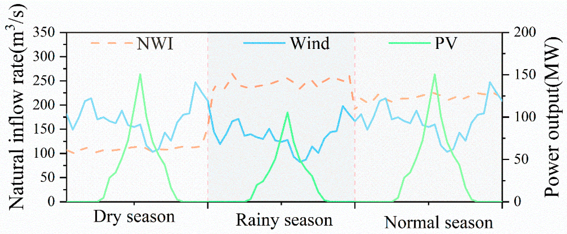
3.1. Comparative Analysis of NWIs, Wind, and Solar Uncertainties in Power System Planning

The variability of NWIs directly impacts the regulation capability of HPHS, while the uncertainties in wind and solar generation significantly influence the system’s load supply capacity and the demand for regulation resources. Generally, the uncertainty of NWIs is characterized by pronounced seasonal and inter-annual variations, with relatively minor intra-day fluctuations [28]. As illustrated in Figure 3, during the dry season, reduced precipitation results in insufficient NWIs, limiting the power generation and regulation capabilities of HPHS. In contrast, during the rainy season, abundant rainfall and snowmelt lead to sufficient NWIs, significantly enhancing the regulation capability of HPHS. To accurately capture the mid-to-long-term uncertainties of NWIs in the planning process, this study divides the entire planning horizon into multiple stages based on inter-annual variations and generates NWI instances for each stage using the Latin hypercube sampling method [32].

In comparison, the uncertainties of wind and solar resources are primarily reflected on intra-day and hourly timescales. Wind power generation typically peaks in the early morning and late evening, with reduced output at midday. Solar PV generation, on the other hand, reaches its maximum at noon and decreases to nearly zero in the morning and evening [29]. Additionally, wind and solar generation are strongly influenced by seasonal factors. For instance, higher wind speeds in winter result in increased fluctuations in wind power output, while longer daylight hours in summer significantly enhance PV generation [30]. These short-term uncertainties directly impact the system’s overall output capacity and regulation needs.

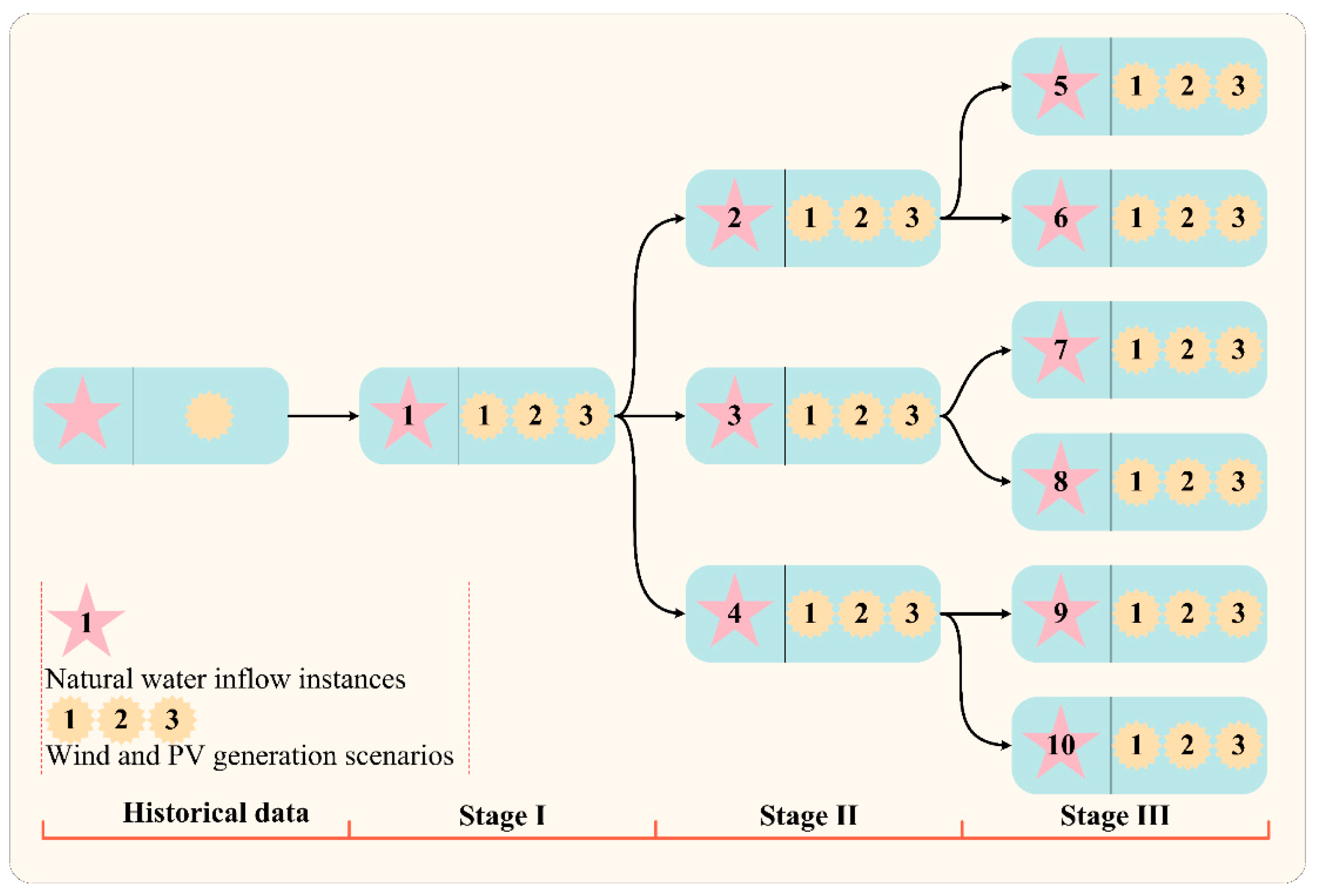
3.2. Handling Inter-Annual and Intra-Day Uncertainties with Instance Trees

To effectively address uncertainties across different timescales, this study proposes a multistage instance tree model with multi-timescale uncertainties, as shown in Figure 4. The inter-annual uncertainties of NWIs are represented as NWI instances, which generate multiple branches under the NACs to capture various long-term variability paths. Within each NWI instance, wind and solar generation scenarios are further generated in order to represent hourly fluctuations, forming a scenario tree for short-term variations. Each NWI instance is designed to accommodate multiple wind and solar scenarios, ensuring an all-scenario feasible planning solution.

Specifically, this study generates a large number of initial scenarios based on the probability distributions of NWIs, as well as wind and solar generation (e.g., wind generation is typically modeled by a Weibull distribution) and historical observational data. To reduce computational complexity while retaining key statistical characteristics, a fast-forward selection method [33] is applied to simplify the initial scenarios. Through scenario filtering and aggregation, a finite set of instances and scenarios is constructed, enabling the resolution of the multi-timescale planning model.

3.3. Non-Anticipativity-Constrained Multistage Optimization

When the uncertainty of NWIs is revealed at stage t, the corresponding unit investment status for that stage can be determined. Additionally, the decision-making process for each NWI instance considers the daily fluctuations in wind and solar power output. Due to the constraints imposed by the NACs, decisions made at each stage depend solely on the currently observable uncertainty realizations. Consequently, as the NWI uncertainties are progressively unveiled, a series of adaptive decision plans can be sequentially generated. This ensures the effectiveness of the proposed approach in addressing both the annual variations in NWIs and the daily fluctuations in wind and solar power output.

Building on this sequential decision-making framework, the proposed method enables dynamic adaptation to unfolding uncertainties. For instance, reservoir operational strategies and capacity expansion plans can be iteratively refined at each stage using updated forecasts for RE generation and NWIs. By incorporating this flexibility, the planning process becomes more robust and cost-effective, ensuring that the system remains resilient across a wide range of future scenarios.

With this foundation, the proposed approach provides a structured methodology for power system planning and scheduling in environments characterized by high renewable energy penetration and significant variability. Accordingly, we formulate the model through Equation (36).

$$\begin{array}{l}\underset{\left\{x_{t,i}\left({\vartheta }_{t,i}\right),y_{t,i}\left({\vartheta }_{t,i}\right)\right\}}{\min }{\displaystyle \sum _{t=1}^{NT}{p}_{t,i}{\displaystyle \sum _{i=1}^K\left(d^T{x}_{t,i}\left({\phi }_{t,i}\right)\right.}}+\left.f_t\left(x_{t,i}\left({\phi }_{t,i}\right),y_{t,i}\left({\phi }_{t,i}\right)\right)\right)\\ s.t. D_t{x}_{t-1,i}\left({\phi }_{t,i}\right)+C_t{x}_{t,i}\left({\phi }_{t,i}\right)=b_t,\forall t,\forall i\\ \left(x_{t,i}\left({\phi }_{t,i}\right),y_{t,i}\left({\phi }_{t,i}\right)\right)ϵ{\Psi }_{t,i}\left({\phi }_{t,i}\right),\forall t,\forall i\\ x_{t,i}\left({\phi }_{t,i}\right)=x_{t,j}\left({\phi }_{t,i}\right),\forall i,jϵ\left\{1,\dots ,K\right\}\cap \left({\phi }_{1,i},\right.\left.\dots ,{\phi }_{t-1,i}\right)=\left({\phi }_{1,j},\dots ,{\phi }_{t-1,j}\right)\end{array}$$

(36)

where $P_{t,i}$ denotes the probability associated with the scenario i at stage t and $d^T{x}_{t,i}\left({\phi }_{t,i}\right)$ represents a linear cost term associated with the variable $x_{t,i}$.

3.4. Implementation of the Proposed Model

The solution procedure is presented as follows:

• Step 1: Multistage Instance Tree Generation

Generate a multistage instance tree based on Section 3.2. This tree reflects various NWI uncertainties through a Monte Carlo simulation. Reduce the number of inflow instances by applying a suitable filtering or clustering technique.

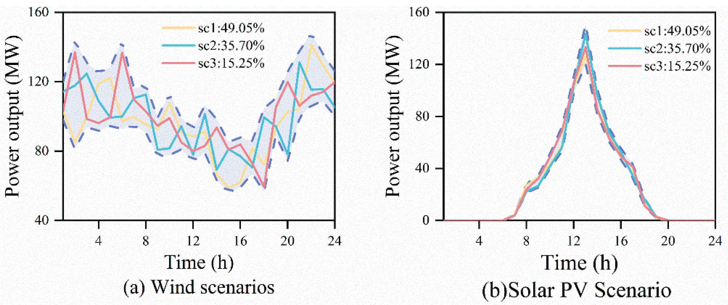
• Step 2: Wind and Solar Scenario Generation

For each NWI instance, generate multiple wind and solar scenarios at specified confidence intervals. Apply the fast-forward scenario reduction method (Section 3.2) to eliminate scenarios with low occurrence probabilities.

• Step 3: Multistage Stochastic Planning

Use the model detailed in Section 3.3 to coordinate system optimization for the scenario tree generated in Step 2. This step determines how investments and operations are adjusted at each stage as uncertainties unfold.

• Step 4: Solution to the Model

Solve the multistage stochastic CHWS-PHS model (Equation (36)) to obtain optimal decisions for both investment and operational stages across all scenarios, ensuring the system remains robust against evolving and diverse conditions.

4. Case Study

In this section, we validate the applicability of the proposed HPHS-AIRC strategy and the MSSP coordinated planning model using both the IEEE 14-bus and IEEE 118-bus systems. Computational experiments are conducted on a PC equipped with an AMD R7-4800H processor (3.2 GHz) and 32 GB RAM, utilizing the commercial solver GUROBI 10.0.1 within MATLAB 2022b for solving the MILP problems. An optimality gap of 0.1% is set to ensure solution precision.

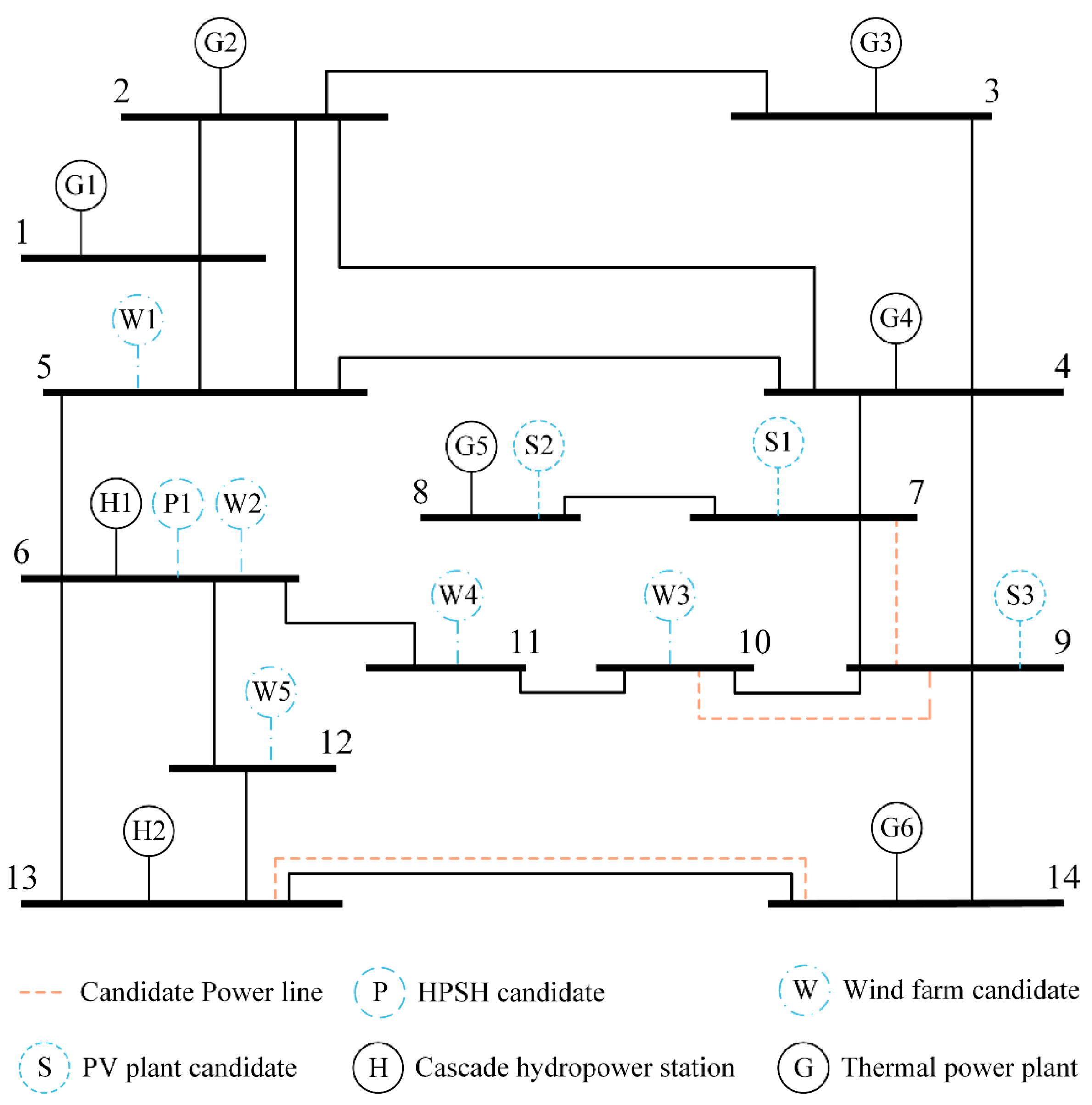
4.1. IEEE 14-Bus System

Figure 5 depicts the IEEE 14-bus CHWS-PHS test system, comprising six thermal generation units (G1–G6) and a two-stage cascade hydropower station. The cascade station features H1 as the upper reservoir and H2 as the lower reservoir. An HPHS candidate (P1) is situated at H1. In addition, five candidate wind farm locations (W1–W5) are provided, each offering three candidate wind units. Similarly, three PV candidate nodes (S1–S3) are available, each with three PV unit options. The figure also shows three candidate transmission lines: L1 (Node 7–9), L2 (Node 9–10), and L3 (Node 13–14).

To account for future scenarios with high wind and solar penetration, this study also considers decommissioning thermal units at predetermined retirement stages.

Table 1. Thermal generator parameters.

Unit	Lower (MW)	Upper (MW)	Ramp (MW/h)	Retirement Stage
G1	25	100	50	2
G2	75	300	150	-
G3	50	200	100	3
G4	100	300	150	2
G5	25	100	50	2
G6	50	250	125	3

lists the key parameters and retirement timelines of the thermal power units, whereas details regarding the cascade hydropower station are documented in [31]. The investment costs for wind farms, PV plants, VS-HPHS [34], and candidate transmission lines [35] are 1056 USD/kW, 639 USD/kW, 662 USD/kW, and 9190.74 USD/line, respectively. To maximize the utilization of wind and solar resources while ensuring a reliable power supply, the cost coefficients for load shedding and RE curtailment are set to 50,000 USD/MWh and 5000 USD/MWh, respectively. A 5% discount rate is applied to compute present values.

The study spans a 15-year planning horizon that is divided into three stages for analysis, with each stage representing a typical 24 h operational window. Consequently, NT = 3 and NK = 24, yielding a 72 h (3 × 24) simulation that captures planning and operational outcomes over 15 years. A 15% load increase is assumed at each stage, and forecast scenarios for NWIs and RE output are generated in accordance with Section 3.1.

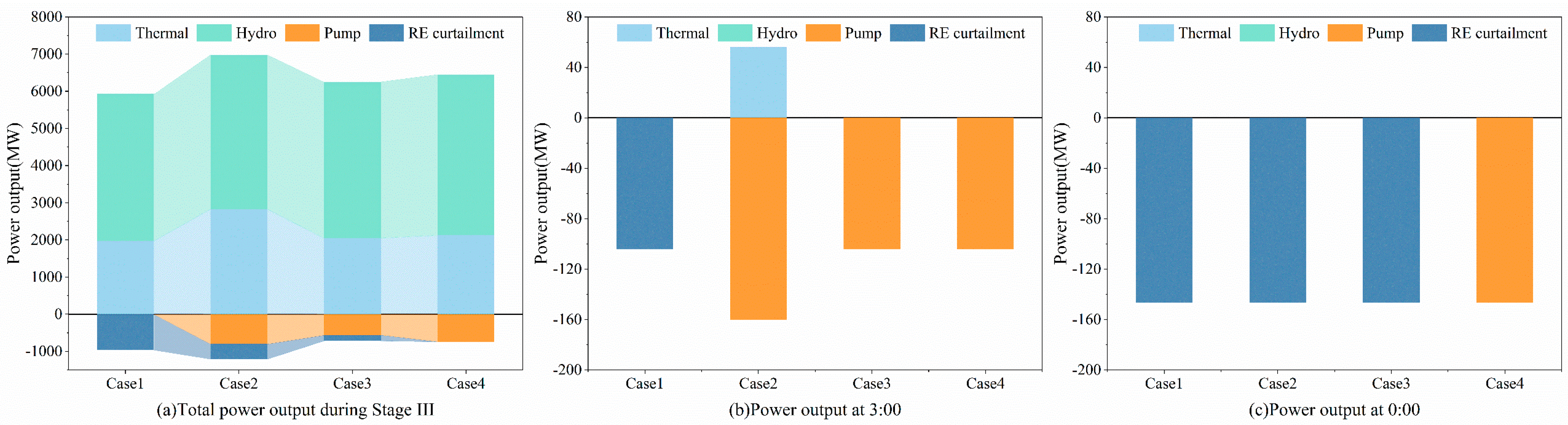
(1)

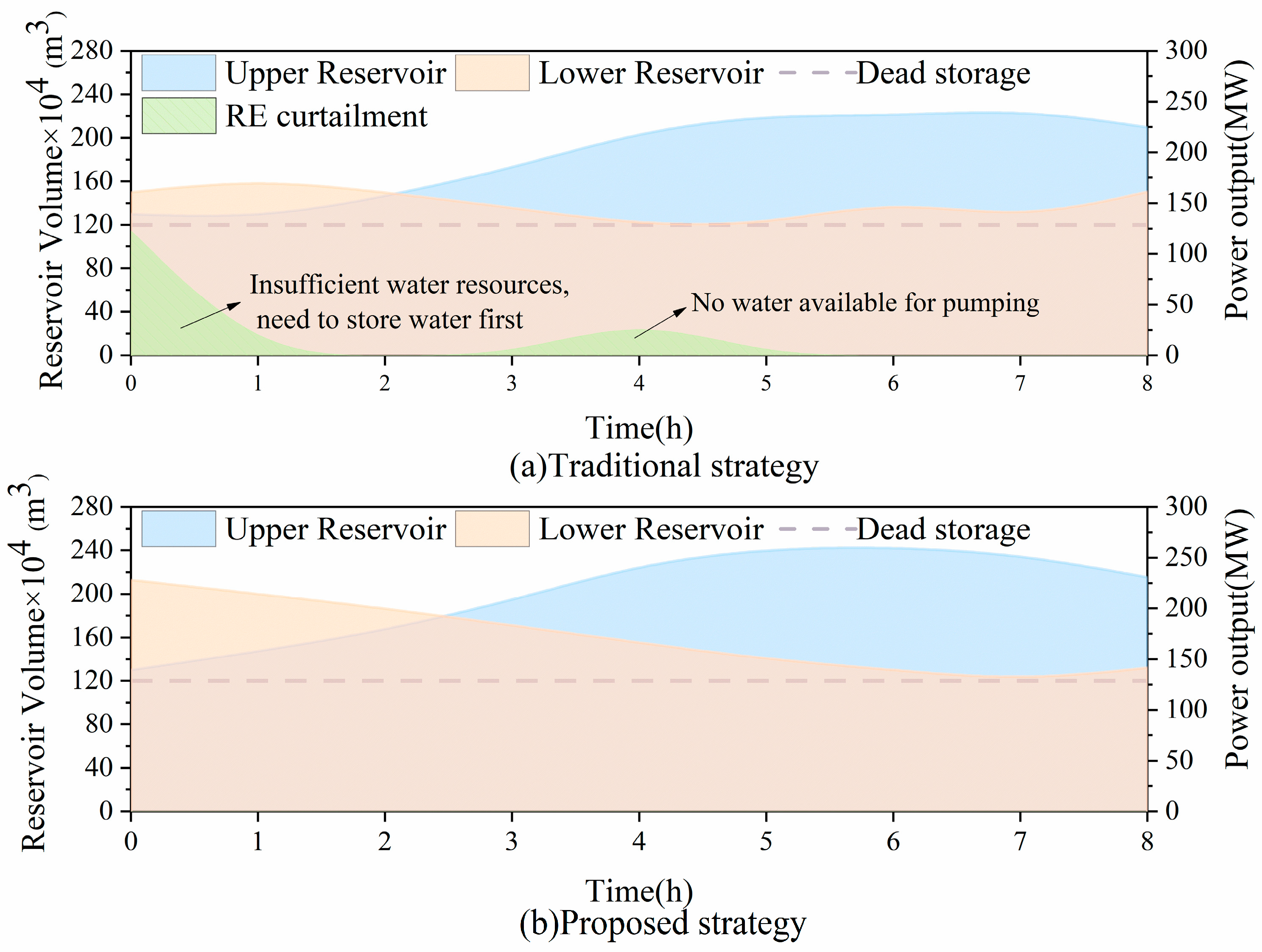
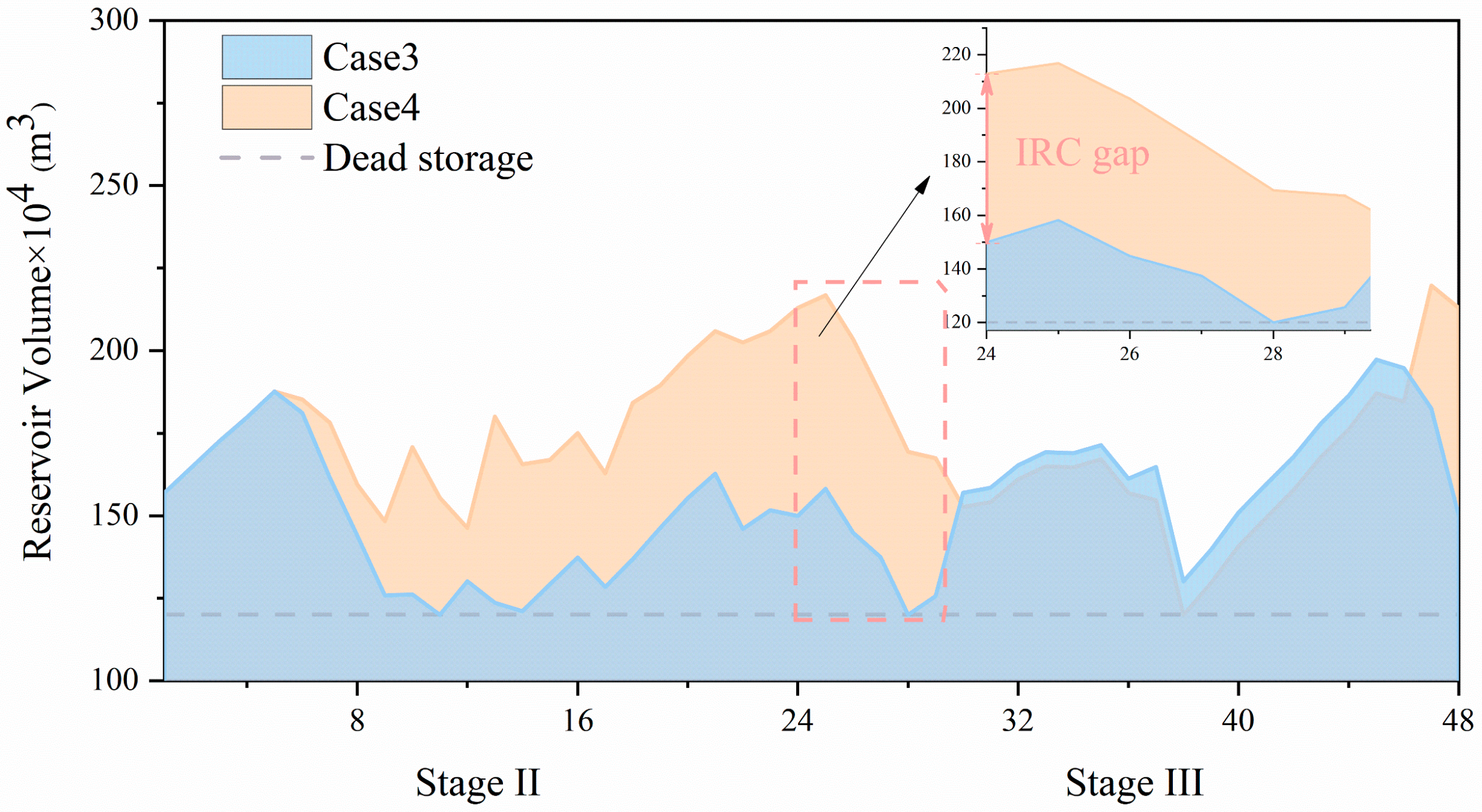
Proposed HPHS-AIRC Strategy

To assess the effectiveness of the HPHS-AIRC strategy, a comparative analysis is conducted under a deterministic scenario using the cases listed in

Table 2. Settings of Cases 1–4.

Case	Type of HPHS		IRC Strategy
	FS	VS	FIRC	HPHS-AIRC
Case 1	-	-	-	-
Case 2	√		√
Case 3		√	√
Case 4		√		√

.

Case 1: This study establishes Case 1 (without PHS) as the baseline case, with its cost results presented in

Table 3. Cost comparison in Cases 1–4.

Cost (USD Billion)	${\mathit{C}}^{\mathbf{I}}$	${\mathit{C}}^{\mathbf{G}}$	${\mathit{C}}^{\mathbf{N}}$	${\mathit{C}}^{\mathbf{L}}$	Total
Case 1	2.30	1.48	5.42	0	9.20
Case 2	2.33	1.49	2.30	0	6.13
Case 3	2.36	1.49	0.82	0	4.67
Case 4	2.36	1.51	0	0	3.87

. Over the entire planning period, Case 1 incurs a total cost of USD 9.20B, of which the penalty cost for RE curtailment accounts for the largest proportion at 58.91% (USD 5.42B), followed by the thermal power operating cost at 16.09% (USD 1.48B).

Figure 6 illustrates the output of each generation unit at different stages during the planning period. As the planning stages progress, thermal power units are gradually retired, with their output share dropping from 73% to 4.6%. Simultaneously, the share of RE generation significantly increases to meet the system’s load demand. However, due to insufficient regulation capability, RE curtailment occurs in Stage III, resulting in substantial penalty costs. Figure 7 illustrates the total power output in Stage III and the outputs at specific representative moments for Cases 1–4. The results indicate that as the share of wind and solar power generation rapidly increases, the system’s flexibility reserves struggle to accommodate the variability of RE, leading to significant RE curtailment at both 0:00 and 3:00, thereby leading to a substantial rise in system costs overall. To address this issue, PHS units need to be installed in Stage III to enhance the system’s flexibility reserves and reduce RE curtailment.

Case 2: To reduce RE curtailment in Stage III, Case 2 transforms the traditional cascade hydropower system in Case 1 into an HPHS system equipped with fixed-speed (FS) PHS units. The results in Table 3 show that the RE curtailment penalty cost in Case 2 decreases to USD 2.30B, representing a 42% reduction compared with Case 1. However, the issue of RE curtailment is not fully resolved. This is primarily due to the startup limitations of FS units, where the pumping power is constrained by Equation (37) and requires meeting the rated power (160 MW) to initiate. When the available RE curtailment at a given moment is insufficient to meet this requirement, curtailment still occurs.

$$P_{t,k,h}^{\mathrm{pump}}=\overline{P_h^{\mathrm{pump}}}{I}_{t,k,h}^{\mathrm{pump}}$$

(37)

As shown in Figure 7a, although the RE curtailment in Case 2 decreases by 42% compared with Case 1, the total thermal power output increases by 43%. This is because the planning objective is to maximize RE utilization. To avoid the significant penalty costs associated with RE curtailment, thermal units in Case 2 provide additional power output to assist the startup of the FS units, thereby completing the RE utilization task at the corresponding moments. For instance, in Figure 7b, at 3:00, Case 1 experiences 104 MW of RE curtailment, close to the 160 MW startup power required for the PHS units. Therefore, the thermal unit in Case 2 generates an additional 56 MW to enable the startup of the PHS units, successfully utilizing the RE output at this time.

Case 3: To address the issues associated with FS units, Case 3 replaces the FS units in Case 2 with variable-speed (VS) units. As shown in Table 3, the RE curtailment cost in Case 3 further decreases to USD 0.82B, representing a 64% reduction compared with Case 2. Additionally, the investment cost increases by USD 0.03B due to the fact that VS units are 42% more expensive than FS units [36]. In Figure 7a, both the thermal power output and the RE curtailment in Case 3 are lower than those in Case 2. Furthermore, Figure 7b shows that the pumping power in Case 3 is lower than in Case 2 and equals the RE curtailment in Case 1, with no thermal power output. This demonstrates the superior regulation capability of VS units, as they overcome the startup limitations of FS units, making VS units a more optimal solution for future high-RE-penetration systems. However, Case 3 still does not fully resolve the issue of RE utilization. For example, Figure 7c shows that at 0:00 in Stage III, Case 3 experiences 146.5 MW of RE curtailment, while the PHS units are not online.

Case 4: To further enhance the regulation capability of VS-HPHS units, the proposed HPHS-AIRC strategy is incorporated into Case 3. The result of Case 4 is shown in Table 3 and Figure 7. The results in Table 3 show that Case 4 completely eliminates the issue of RE curtailment, with the total cost reduced to USD 3.87 billion. As can also be seen in Figure 7c, Case 4 does not generate RE curtailment at 0:00. To further analyze the reason for this phenomenon, Figure 8 presents the reservoir volume curve of the lower hydro unit. At 0:00, during Stage III, the reservoir volume in Case 4 is $60\times {10}^4 {\mathrm{m}}^3$ higher than Case 3, allowing it to meet the pump demand. With the proposed HPHS-AIRC strategy, water demand of the lower reservoir is elevated during Stage II, leading to a reduction in overall hydropower output; this adjustment does not significantly increase the burden on thermal units. The total thermal power cost only rises by USD 0.02B while ensuring the complete utilization of wind and solar energy. This demonstrates that the HPHS-AIRC strategy, by optimizing the IRC and managing reservoir capacity scheduling, enhances system flexibility.

(2)

MSSP with NACs

To analyze the impact of the uncertainties in wind, solar, and NWIs mentioned in Section 3.3 on the planning results and to validate the effectiveness of the multistage coordinated planning model proposed in this paper, other cases are implemented based on Case 4, as listed in

Table 4. Uncertainty and planning method settings for Cases 5–7.

Case	Uncertainty		Model
	NWI	RE	TSSP	MSSP
Case 5	√		√
Case 6	√			√
Case 7	√	√		√

.

Case 5: This case serves as the baseline case built using the TSSP model. It considers the impact of NWI instances and their inter-annual variability on investment results, based on Case 4. Starting with a normal NWI instance in Stage I, the model branches into flood, normal, and drought conditions in Stage II and further diversifies in Stage III. Figure 9 illustrates the resulting three-stage NWI instance tree and the probability of each instance.

The total cost for Case 5 is USD 3.94B, with thermal power operating costs of USD 1.57B and total investment costs of USD 2.36B. Notably, thermal power operating costs increased by USD 0.06B due to the added uncertainty in NWIs. The investment decision results are shown in Figure 10a. Since the traditional TSSP model cannot adjust its investment decisions dynamically as uncertainties unfold, only a single investment plan is provided for each NWI instance in this case.

Case 6: To demonstrate the impact of the MSSP method with NACs on investment outcomes, Case 6 considers the same NWI instances as Case 5. The results show that the total cost of Case 6 is USD 3.85B, with investment costs of USD 2.19B and thermal power costs of USD 1.65B. The investment cost in Case 6 is USD 0.17B lower than in Case 5. To further explain this reduction, Figure 10b shows the unit investment decisions for Case 6 corresponding to each NWI instance. Case 6 makes one decision in Stage I; three decisions in Stage II, corresponding to drought, flood, and normal conditions; and six decisions in Stage III, corresponding to six different NWI instances. Due to the influence of NACs, for the same revealed uncertainty, such as evolutionary paths $\mathrm{①}\to \mathrm{②}\to \mathrm{⑤}$ and $\mathrm{①}\to \mathrm{②}\to \mathrm{⑥}$, the decisions made in the first two stages are identical and unaffected by the third-stage instances $\mathrm{⑤}$ and $\mathrm{⑥}$.

Furthermore, as shown in Figure 10, there were seven wind turbines installed in Stage II for Case 5, while in two of the three decision sets for Case 6, only six turbines were installed. In Stage III, three PV units were installed in Case 5, whereas in Case 6, only one PV unit was installed in instance $\mathrm{⑤}$. This suggests that the investment decisions generated by Case 5 for these scenarios are either unsuitable or not optimal. In fact, as NWI uncertainty is revealed over multiple years, the corresponding investment decisions should continuously adapt. The MSSP model, considering NACs, can make different investment decisions based on varying uncertainties, allowing it to better handle different uncertainty scenarios and achieve better cost outcomes.

Case 7: To further illustrate the impact of short-term fluctuations in wind and solar output on planning and scheduling results, Case 7 incorporates additional wind and solar uncertainties based on Case 6. The wind and solar output scenarios were generated using a 90% confidence interval to model the uncertainty of wind and solar resources in each NWI instance. A total of 2000 wind and solar output scenarios were generated, and scenario reduction techniques were applied to retain 3 representative scenarios. Figure 11 presents the resulting wind and solar power scenarios.

The costs for Case 7 are as follows: investment cost is USD 2.59B, thermal power generation cost is USD 1.70B, RE curtailment cost is USD 1.18B, load shedding cost is USD 0, and the total cost is USD 5.47B. Compared with Case 6, the investment cost increases by USD 0.40B, and thermal power operating costs rise by USD 0.05B. Additionally, an RE curtailment penalty of USD 1.18B occurs due to the increased volatility of wind and solar generation. As the fluctuations become more severe, the wind and solar generation in certain time periods exceeds the maximum pumping capacity of the HPHS units, resulting in excess wind and solar power being curtailed. Furthermore, the wind and solar output also impacts on the system’s ability to meet load requirements, with thermal units needing to produce more power to satisfy the generation demand.

Although the costs in Case 7 are higher compared with Case 6, the decisions in Case 7 are better adapted to the daily fluctuations in wind and solar generation, leading to better scenario feasibility. Additionally, the load shedding penalty remains zero, indicating that the model proposed in this study can still meet the power system’s supply–demand balance, even when facing a combination of multiple uncertainties.

4.2. Application of MSSP in the IEEE 118-Bus System

To further demonstrate the scalability and practicality of the proposed HPHS-AIRC strategy and the MSSP model, we apply them to the more complex IEEE 118-bus system. The IEEE 118-bus test system consists of 48 thermal generators distributed across various locations and nine two-stage cascade hydropower stations, each with upper reservoirs designated as candidate HPHS nodes. Additionally, the system includes 37 candidate wind farm locations and 32 candidate PV plant sites, with each site capable of accommodating up to three wind turbines or PV units. The generator parameters mirror those of the IEEE 14-bus system, ensuring consistency in model validation.

In this system, case studies similar to the IEEE 14-bus system were set up, primarily focusing on Case 3 to Case 7 for analysis.

Table 5. Results comparison for the IEEE 118-bus system.

Case	${\mathit{C}}^{\mathbf{I}}$ (USD Billion)	${\mathit{C}}^{\mathbf{G}}$ (USD Billion)	${\mathit{C}}^{\mathbf{N}}$ (USD Billion)	${\mathit{C}}^{\mathbf{L}}$ (USD Billion)	Total (USD Billion)	${\mathit{P}}^{\mathbf{pump}}$ (MW)	Time (s)
Case 3	16.94	11.96	4.04	0	32.94	5671	113
Case 4	16.94	12.19	0	0	29.13	7587	110
Case 5	17.45	11.16	2.11	0	30.72	-	1142
Case 6	17.26	11.54	0	0	28.80	-	2731
Case 7	18.55	12.54	1.04	0	32.13	-	6482

presents the computational costs and efficiency information for each case.

As shown in Table 5, Case 4 reduces wind and solar curtailment by 100% with only a 1.9% increase in thermal power operating costs. The total utilization rate of HPHS for typical daily periods improves by 33.8%. This indicates that, after adopting the HPHS-AIRC strategy, HPHS units can fully utilize their potential without being limited by insufficient water resources, thereby maximizing the integration of wind and solar power. This highlights the effectiveness of the HPHS-AIRC strategy.

In addition, we set Case 5 and Case 6 to compare the advantages of the MSSP model in addressing uncertainty with NACs, where only NWI uncertainty was considered. Case 6 achieved better investment and operational costs compared with Case 5, with a reduction in investment cost by USD 0.19B and the avoidance of RE curtailment penalties. This indicates that the MSSP model, when used for long-term planning, can generate more optimal investment decisions for different scenarios, leading to better operational performance and lower penalties. Furthermore, in terms of computational time, Case 6 only took 26 min longer than Case 5. Such a difference in computational time is entirely acceptable for long-term planning.

Finally, we set up Case 7, which resulted in an investment cost of USD 18.55B, a thermal generation operational cost of USD 12.54B, and RE curtailment penalties of USD 1.04B. It can be observed that when the intra-day fluctuations of wind and solar power output are additionally considered, all system costs increase, and the computational time extends to 6482 s. However, overall, these increases in cost and computational time remain entirely acceptable.

The results obtained for the IEEE 118-bus system are generally consistent with the conclusions derived from the IEEE 14-bus system, thereby validating the effectiveness of the proposed HPHS-AIRC strategy in enhancing the regulation capability of HPHS. Furthermore, the findings demonstrate the efficacy of the MSSP model with NACs in addressing multi-timescale uncertainties.

5. Discussion

5.1. Advantages of the HPHS-AIRC Strategy

The results from Cases 1–4 reveal that traditional fixed-speed PHS units have inherent limitations in RE absorption due to startup constraints. Replacing them with VS units reduces RE curtailment significantly. Furthermore, by introducing the HPHS-AIRC strategy in Case 4, the curtailment is completely eliminated. This is attributed to the strategy’s ability to flexibly coordinate reservoir volumes and pumping schedules across planning stages, thus enhancing regulation capability without significantly increasing thermal generation costs.

5.2. Impact of Uncertainty and MSSP Modeling

The performance of Cases 5–7 demonstrates the effectiveness of the MSSP model with NACs in improving long-term investment decisions under uncertainty. Case 6, with MSSP and NACs, achieves better cost performance than Case 5 with the traditional TSSP model, by enabling scenario-dependent but temporally consistent decisions. Case 7 further shows that while incorporating RE uncertainty increases the total cost and computational time, it also enhances the robustness and feasibility of the decisions, as evidenced by zero load shedding and reduced infeasibility under extreme scenarios.

5.3. Scalability and Practicality in Larger Systems

The extension to the IEEE 118-bus system confirms the scalability of the proposed approach. The HPHS-AIRC strategy consistently improves RE utilization, and the MSSP model proves capable of managing complex multi-year, multi-scenario decisions. The additional computational time required is acceptable for long-term planning purposes.

6. Conclusions

In this paper, we propose a multistage stochastic coordinated planning model for the CHWS-PHS system to address the impact of uncertainty across different timescales on system planning. Additionally, an HPHS-AIRC strategy is introduced to enhance the regulation ability of the HPHS. The proposed model adjusts investment strategies as uncertainty is revealed, ensuring that the strategies formulated at each stage remain optimal. Moreover, the HPHS-AIRC strategy improves the regulation capability of PHS units, especially in scenarios with arid conditions or difficulties in unit startup. By proactively adjusting the reservoir capacity scheduling, the strategy enhances the regulation ability of PHS in these challenging scenarios.

Simulation results for the IEEE 118-bus system indicate that: (1) the HPHS-AIRC strategy significantly improves the regulation ability of PHS, particularly under drought conditions or for units with insufficient regulation capacity, leading to a 33.8% increase in PHS utilization under identical conditions. (2) The proposed MSSP coordinated planning model provides distinct investment decisions for uncertain scenarios that unfold over time, resulting in a 6% reduction in the total cost compared with the TSSP model. (3) Although the computational time of the MSSP model reaches twice that of TSSP, the gap remains at an hour-level scale. Even when addressing more complex uncertainty scenarios, the final solution time is limited to 1.8 h, which remains acceptable for planning cycles.

While this study demonstrates the efficacy of the HPHS-AIRC strategy and the MSSP model in improving PHS regulation and cost-effective planning under uncertainty, several promising directions remain:

(1)

Topology Scalability: The current framework assumes a simplified PHS configuration. Future work could extend the HPHS-AIRC strategy to multistage cascaded reservoirs to evaluate its performance in complex hydropower topologies, where hydraulic coupling and sequential water-outflow constraints may challenge regulation stability.

(2)

Parameter Adaptability: The impact of adaptive control parameters δ_pump on regulation capability warrants systematic analysis. A sensitivity-driven parameter optimization framework could further enhance the strategy’s robustness across diverse operating scenarios.

References

- Virah-Sawmy, D.; Sturmberg, B. Socio-economic and environmental impacts of renewable energy deployments: A review. Renew. Sustain. Energy Rev. 2025, 207, 114956. [Google Scholar] [CrossRef]
- Mitchell, C. Momentum is increasing towards a flexible electricity system based on renewables. Nat. Energy 2016, 1, 15030. [Google Scholar] [CrossRef]
- Qiu, X.; Chen, Y.; Cai, W.; Niu, M.; Li, J. LD-YOLOv10: A Lightweight Target Detection Algorithm for Drone Scenarios Based on YOLOv10. Electronics 2024, 13, 3269. [Google Scholar] [CrossRef]
- Bhandari, B. A novel off-grid hybrid power system comprised of solar photovoltaic, wind, and hydro energy sources. Appl. Energy 2014, 133, 236–242. [Google Scholar] [CrossRef]
- Gielen, D.; Boshell, F.; Saygin, D.; Bazilian, M.D.; Wagner, N.; Gorini, R. The role of renewable energy in the global energy transformation. Energy Strategy Rev. 2019, 24, 38–50. [Google Scholar] [CrossRef]
- Shair, J. Power system stability issues, classifications and research prospects in the context of high-penetration of renewables and power electronics. Renew. Sustain. Energy Rev. 2021, 145, 111111. [Google Scholar] [CrossRef]
- Sterl, S. Smart renewable electricity portfolios in West Africa. Nat. Sustain. 2020, 3, 710–719. [Google Scholar] [CrossRef]
- Rana, M.M.; Uddin, M.; Sarkar, M.R.; Meraj, S.T.; Shafiullah, G.M.; Muyeen, S.M.; Islam, M.A.; Jamal, T. Applications of energy storage systems in power grids with and without renewable energy integration—A comprehensive review. J. Energy Storage 2023, 68, 107811. [Google Scholar] [CrossRef]
- Javed, M.S.; Zhong, D.; Ma, T.; Song, A.; Ahmed, S. Hybrid pumped hydro and battery storage for renewable energy based power supply system. Appl. Energy 2020, 257, 114026. [Google Scholar] [CrossRef]
- Barbour, E.; Wilson, I.A.G.; Radcliffe, J.; Ding, Y.; Li, Y. A review of pumped hydro energy storage development in significant international electricity markets. Renew. Sustain. Energy Rev. 2016, 61, 421–432. [Google Scholar] [CrossRef]
- Tan, Q.; Nie, Z.; Wen, X.; Su, H.; Fang, G.; Zhang, Z. Complementary scheduling rules for hybrid pumped storage hydropower-photovoltaic power system reconstructing from conventional cascade hydropower stations. Appl. Energy 2024, 355, 122250. [Google Scholar] [CrossRef]
- Acuña, G.; Domínguez, R.; Arganis, M.L.; Fuentes, O. Optimal Schedule the Operation Policy of a Pumped Energy Storage Plant Case Study Zimapán, México. Electronics 2022, 11, 4139. [Google Scholar] [CrossRef]
- Sospiro, P.; Nibbi, L.; Liscio, M.C.; De Lucia, M. Cost–Benefit Analysis of Pumped Hydroelectricity Storage Investment in China. Energies 2021, 14, 8322. [Google Scholar] [CrossRef]
- Zhang, X. Capacity configuration of a hydro-wind-solar-storage bundling system with transmission constraints of the receiving-end power grid and its techno-economic evaluation. Energy Convers. Manag. 2022, 270, 116177. [Google Scholar] [CrossRef]
- Sun, K.; Li, K.-J.; Pan, J.; Liu, Y.; Liu, Y. An optimal combined operation scheme for pumped storage and hybrid wind-photovoltaic complementary power generation system. Appl. Energy 2019, 242, 1155–1163. [Google Scholar] [CrossRef]
- Zhang, S.; Xiang, Y.; Liu, J.; Liu, J.; Yang, J.; Zhao, X.; Jawad, S.; Wang, J. A Regulating Capacity Determination Method for Pumped Storage Hydropower to Restrain PV Generation Fluctuations. Csee J. Power Energy Syst. 2022, 8, 304–316. [Google Scholar]
- Hunt, J.D.; Freitas, M.A.V.; Pereira Junior, A.O. Enhanced-Pumped-Storage: Combining pumped-storage in a yearly storage cycle with dams in cascade in Brazil. Energy 2014, 78, 513–523. [Google Scholar] [CrossRef]
- Ak, M. Quantifying the revenue gain of operating a cascade hydropower plant system as a pumped-storage hydropower system. Renew. Energy 2019, 139, 739–752. [Google Scholar] [CrossRef]
- Lu, M.; Guan, J.; Wu, H.; Chen, H.; Gu, W.; Wu, Y.; Ling, C.; Zhang, L. Day-ahead optimal dispatching of multi-source power system. Renew. Energy 2022, 183, 435–446. [Google Scholar] [CrossRef]
- Zhang, J.; Cheng, C.; Yu, S.; Shen, J.; Wu, X.; Su, H. Preliminary feasibility analysis for remaking the function of cascade hydropower stations to enhance hydropower flexibility: A case study in China. Energy 2022, 260, 125163. [Google Scholar] [CrossRef]
- Wang, Z.; Fang, G.; Wen, X.; Tan, Q.; Zhang, P.; Liu, Z. Coordinated operation of conventional hydropower plants as hybrid pumped storage hydropower with wind and photovoltaic plants. Energy Convers. Manag. 2023, 277, 116654. [Google Scholar] [CrossRef]
- Niknam, T. An efficient scenario-based stochastic programming framework for multi-objective optimal micro-grid operation. Appl. Energy 2012, 99, 455–470. [Google Scholar] [CrossRef]
- Park, H. Multi-year stochastic generation capacity expansion planning under environmental energy policy. Appl. Energy 2016, 183, 737–745. [Google Scholar] [CrossRef]
- Mavromatidis, G.; Orehounig, K.; Carmeliet, J. Design of distributed energy systems under uncertainty: A two-stage stochastic programming approach. Appl. Energy 2018, 222, 932–950. [Google Scholar] [CrossRef]
- Ding, T.; Hu, Y.; Bie, Z. Multi-Stage Stochastic Programming With Nonanticipativity Constraints for Expansion of Combined Power and Natural Gas Systems. IEEE Trans. Power Syst. 2018, 33, 317–328. [Google Scholar] [CrossRef]
- Zhang, G.; Zhang, F.; Zhang, X.; Wang, Z.; Meng, K.; Dong, Z.Y. Mobile Emergency Generator Planning in Resilient Distribution Systems: A Three-Stage Stochastic Model With Nonanticipativity Constraints. IEEE Trans. Smart Grid 2020, 11, 4847–4859. [Google Scholar] [CrossRef]
- Cobos, N.G. Network-constrained unit commitment under significant wind penetration: A multistage robust approach with non-fixed recourse. Appl. Energy 2018, 232, 489–503. [Google Scholar] [CrossRef]
- Rahat, S.H.; Steissberg, T.; Chang, W.; Chen, X.; Mandavya, G.; Tracy, J.; Wasti, A.; Atreya, G.; Saki, S.; Bhuiyan, A.E.; et al. Remote sensing-enabled machine learning for river water quality modeling under multidimensional uncertainty. Sci. Total Environ. 2023, 898, 165504. [Google Scholar] [CrossRef]
- Prasad, A.A.; Taylor, R.A.; Kay, M. Assessment of solar and wind resource synergy in Australia. Appl. Energy 2017, 190, 354–367. [Google Scholar] [CrossRef]
- Heide, D.; Von Bremen, L.; Greiner, M.; Hoffmann, C.; Speckmann, M.; Bofinger, S. Seasonal optimal mix of wind and solar power in a future, highly renewable Europe. Renew. Energy 2010, 35, 2483–2489. [Google Scholar] [CrossRef]
- Yin, Y.; Liu, T.; He, C. Day-ahead stochastic coordinated scheduling for thermal-hydro-wind-photovoltaic systems. Energy 2019, 187, 115944. [Google Scholar] [CrossRef]
- Straume, M.; Johnson, M.L. [7] Monte Carlo Method for determining complete confidence probability distributions of estimated model parameters. In Methods in Enzymology; Elsevier: Amsterdam, The Netherlands, 1992; Volume 210, pp. 117–129. [Google Scholar] [CrossRef]
- Wu, L.; Shahidehpour, M.; Li, Z. GENCO’s Risk-Constrained Hydrothermal Scheduling. IEEE Trans. Power Syst. 2008, 23, 1847–1858. [Google Scholar] [CrossRef]
- Liu, Z.; He, X. Balancing-oriented hydropower operation makes the clean energy transition more affordable and simultaneously boosts water security. Nat. Water 2023, 1, 778–789. [Google Scholar] [CrossRef]
- Alnowibet, K.A.; Alrasheedi, A.F.; Alshamrani, A.M. Integrated stochastic transmission network and wind farm investment considering maximum allowable capacity. Electr. Power Syst. Res. 2023, 215, 108961. [Google Scholar] [CrossRef]
- Zhao, Z. Beyond fixed-speed pumped storage: A comprehensive evaluation of different flexible pumped storage technologies in energy systems. J. Clean. Prod. 2024, 434, 139994. [Google Scholar] [CrossRef]