PV Production Forecast Using Hybrid Models of Time Series with Machine Learning Methods

Abstract

Photovoltaic (PV) energy production in Western countries increases yearly. Its production can be carried out in a highly distributed manner, not being necessary to use large concentrations of solar panels. As a result of this situation, electricity production through PV has spread to homes and open-field plans. Production varies substantially depending on the panels’ location and weather conditions. However, the integration of PV systems presents a challenge for both grid planning and operation. Furthermore, the predictability of rooftop-installed PV systems can play an essential role in home energy management systems (HEMS) for optimising local self-consumption and integrating small PV systems in the low-voltage grid. In this article, we show a novel methodology used to predict the electrical energy production of a 48 kWp PV system located at the Campus Feuchtwangen, part of Hochschule Ansbach. This methodology involves hybrid time series techniques that include state space models supported by artificial intelligence tools to produce predictions. The results show an accuracy of around 3% on nRMSE for the prediction, depending on the different system orientations.

1. Introduction

The installed PV capacity in Europe has risen dramatically from 30 GWp in 2010 to over 250 GWp in 2022 [1]. By the end of 2024, Germany alone has installed 99 GWp. With the goal of achieving climate neutrality, the installed capacity in Germany is expected to reach up to 400 GWp by 2040 [2]. A significant advantage of PV systems is their low levelized cost of electricity (LCOE) [3]. Additionally, the nominal efficiency rate is increasing by 0.4 percentage points annually, with current average efficiencies around 21% [4]. Integrating up to 400 GWp of PV generation compared to a load of 80 GW is already a challenge in Germany, especially in the low-voltage grids and strong rural regions.

Apart from participation in the day-ahead market, PV forecasting will play an essential role in the operation of low-voltage grids to implement §9EEG. The grid-friendly operation requires local generation and consumption forecasts. However, the accuracy of forecasts for this application is still a relevant but open question. On the other hand, cost-optimised self-consumption in buildings is already playing a significant role [5]. Battery storage systems typically enable this. Additional options for optimised PV self-consumption include battery electric vehicles (BEVs) as well as heat pumps, which are so-called flexible consumers [6]. The optimised control of flexible consumers requires an energy management system (EMS) or, with a focus on single-family households, home energy management systems (HEMS) [7]. The challenge of providing sufficiently precise forecasts for this purpose remains an open research question. In the past, production with traditional generation methods based on thermal sources and very stable prediction gave way to systems that depended on the weather in addition to the functional state of the facilities [8]. The continued increase in generation from renewable sources has led to an increase in the prediction error that has doubled in the last five years and continues to increase [9]. According to the International Energy Agency (IEA), in 2015, there was a production capacity of 196 GW using PV, and a capacity of between 400 and 800 GW was planned for 2020 [10]. The solution consists of having backup systems generally based on batteries and natural gas power plants, which are expensive [11]. Production stability is also a critical point in prediction. Clear lighting conditions are constant in southern European climates, with little cloud cover. In Central Europe, this cloudiness is highly variable, where up to 1/3 of the days of the year can be reached with high cloudiness. This further increases the difficulty of making predictions [12].

In contrast to the systems that are mounted on pitched roofs and point in the direction of the roof, flat roofs offer more degrees of freedom. One of the challenges—also with the system installed on the Campus Feuchtwangen (49°10′47.3′′ N 10°20′07.9′′ E)—is that the orientation of the production units not uniform but is distributed along the roof with varying orientations, making it impossible to use global irradiance as a basis for calculation for predicting energy production. For this reason, statistical methods were used for this task. However, given the complexity of the prediction, which must include environmental factors and a high degree of randomness in the observed data, it was decided to include a layer of machine learning that could complement the predictions. The result is a hybrid model that provides predictions at a considerable level.

This article presents the forecasting method developed at Campus Feuchtwangen for predicting photovoltaic energy production in a solar panel system with an unconventional physical configuration. In this context, traditional models based on solar position and panel inclination are not applicable due to the atypical spatial arrangement of the panels. Moreover, standard time series forecasting techniques have not provided satisfactory results in capturing the system’s production dynamics.

To address these limitations, a novel hybrid modelling approach is proposed. The model integrates state-space representations to internalise the systematic component of energy production, while artificial intelligence techniques are employed to capture and predict the more variable, weather-dependent aspects. This dual-structure framework enables accurate forecasting even under the complex conditions imposed by the system’s unique layout, offering a significant methodological contribution to the field of photovoltaic energy prediction.

It is structured as follows: Section 2 analyses the related work to this article; Section 3 explains the methods used in the article that led to the results shown in Section 4. Section 5 and Section 6 discuss the results and draw conclusions.

2. Related Work

The application of PV forecasts is often discussed in the context of HEMS for optimised PV self-consumption. On the one hand, HEMS are simulated in models where perfect forecasts are used for optimisation [5] or focusing on data prediction using rolling horizons within a 24-h timeframe [6]. A study surveying the practical implementation of 26 HEMS manufacturers revealed that over 50% of these systems currently incorporate PV forecasts [7].

An exact PV forecast will be the prevention of the curtailment of PV systems by §9EEG. By forecasting generation over the 24 h ahead, flexible consumers and their storage systems can be controlled to match. However, an intriguing and unresolved issue is the temporal resolution of these forecasts and how they are integrated into the optimisation algorithms. Another critical and increasingly significant aspect is the inclusion of demand forecasts for electricity and heat, and generation forecasts.

The objective of accurate PV power forecasting models plays a crucial role in ensuring reliable estimates of solar energy output. That forecasting capability is fundamental not only to the strategic planning of HEMS, but also rural electrification initiatives, solar-based irrigation systems, and comprehensive sustainable development efforts, particularly in socioeconomically vulnerable areas. It could effectively mitigate energy poverty while simultaneously contributing to climate resilience [8].

Reviews of PV forecasts have been abundant recently [9,10]. There is a growing interest in improving predictions, as a considerable increase in installed capacity is expected [11].

Production prediction is generally developed from irradiance prediction, especially global horizontal irradiance (GHI). However, it should be noted that energy production efficiency is independent of GHI, although it is correlated with temperature—a relationship that depends on the specific photovoltaic cell technology employed [12]. Other variables affect it, such as cloudiness, but the main one is the GHI. The models usually distinguish between a structural part with Irradiance and another stochastic part where time series models and other methodologies are used [13]. Wu et al. [14] analyse the methods applied to predict solar production. A distinction is made between methods based on time series and machine learning. The former is based on statistical models to determine the new predictions, such as exponential smoothing or ARIMA models. The second group is very varied, highlighting neural network, ensemble, and deep learning models. However, hybrid models stand out. Probabilistic models are also emerging as a new alternative. However, time series models in this type of task are usually combined with elements of machine learning [15].

Kavakci et al. [16] use a hybrid prediction method using time series decomposition; it models the trend as a stable element. It uses ML to model the seasonal and stochastic parts. Aziz and Chowdhury [17] apply ARIMA models for production prediction in Bangladesh. This process is more straightforward, where they use prior information to make univariate predictions. Chodakowska et al. [18] applies SARIMAX models to Jordan and Poland PV stations.

However, there is an incipient growth of academic interest in the development of machine-learning models in this area. Saigustia and Pijarski [19] use XGBoost to determine production in Spain. The results shown are exceptional in terms of fit, although no prediction results are shown. Currently, Long Short-Term Memory (LSTM) Networks and their derivatives are the models that show the most accurate results compared to the rest of the models [20,21]. Scott et al. [22] developed random forest (RF), NN, SVM, and LR models for prediction in different locations, such as Denmark, Holland, America, and Portugal. The proposed models can improve and reduce by half the error measured in terms of RMSE. Boujoudar et al. [23] use Catboost, LightGBM, XGboost and Random Forest to make predictions in semi-arid climate locations, finding that LightGBM outperformed the other models.

One of the main aspects of prediction is the prediction horizon. Predictions can be made for the short or long term. The short-term forecasts (one day ahead) are used for planning, while the former is used for specific operations, with the most common being predictions for one day ahead [24].

3. Materials and Methods

The Campus Feuchtwangen (Bavaria, Germany) has been operational as research building since 2018. This facility collects comprehensive data encompassing thermal, electrical, and environmental parameters such as temperature, humidity, and light levels. Additionally, the site is equipped with two independent weather stations that measure various meteorological data, including solar radiation, temperature, humidity, and wind. All this data is logged at one-minute intervals, providing a detailed and continuous record. Additionally, the site is integrated with the Sector Coupling Laboratory (Feuchtwangen, Germany).

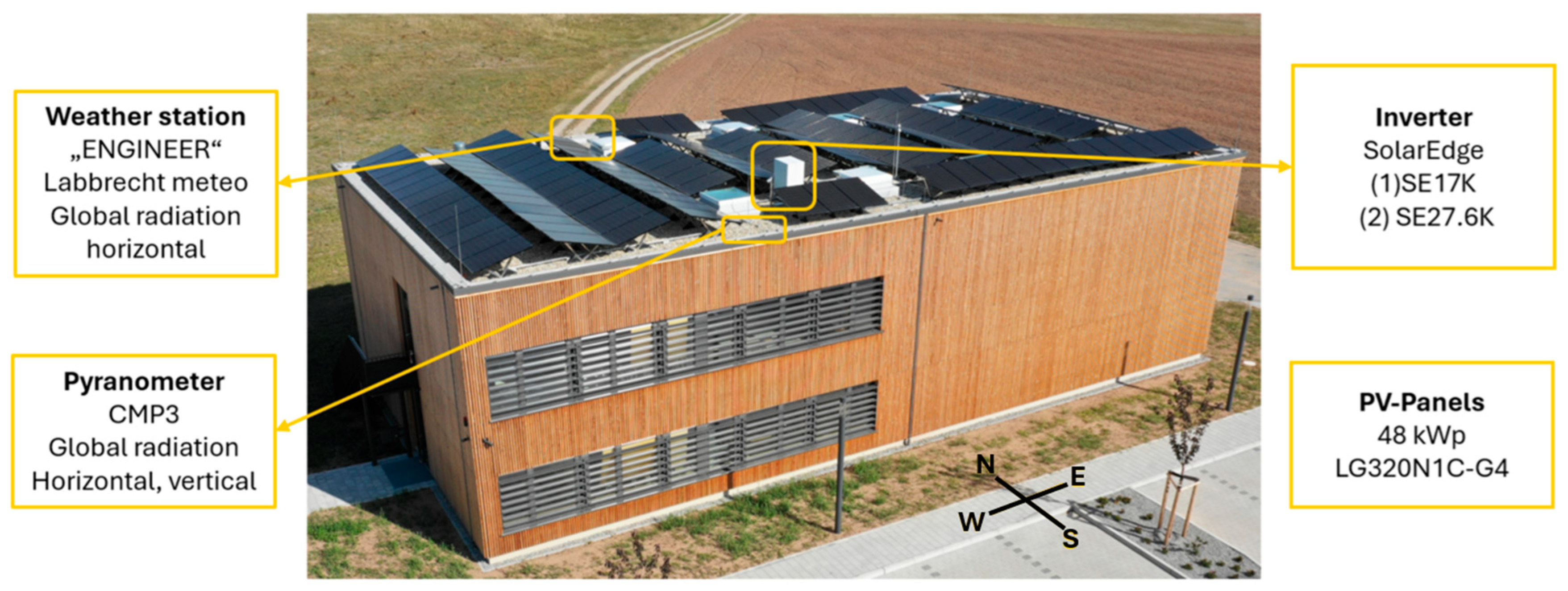
This laboratory connects flexible loads such as battery storage systems, heat pumps, and charging stations for electric vehicles. Figure 1 pictures this installation. The long-term objective is to optimise the operation of these interconnected systems using forecast data from HEMS.

The PV system has a total module capacity of 48 kWp. The design has a mixed orientation to increase the self consumption. It consists of 150 modules of the type LG320N1C-G4. The system is divided into two subsystems. System 1 has a module capacity of 20 kWp and uses a 17-kW inverter (SolarEdge 17K). It includes two strings with 31 modules each (9.92 kWp per string), both facing west. System 2 has a module capacity of 28 kWp and a 27.6 kW inverter (SolarEdge 27.6K). It consists of three strings: one with 27 modules facing south (8.64 kWp), one with 32 modules facing east (10.24 kWp), and one with 29 modules also facing east (9.28 kWp). Each module is equipped with a power optimiser (SolarEdge P370) to improve system performance.

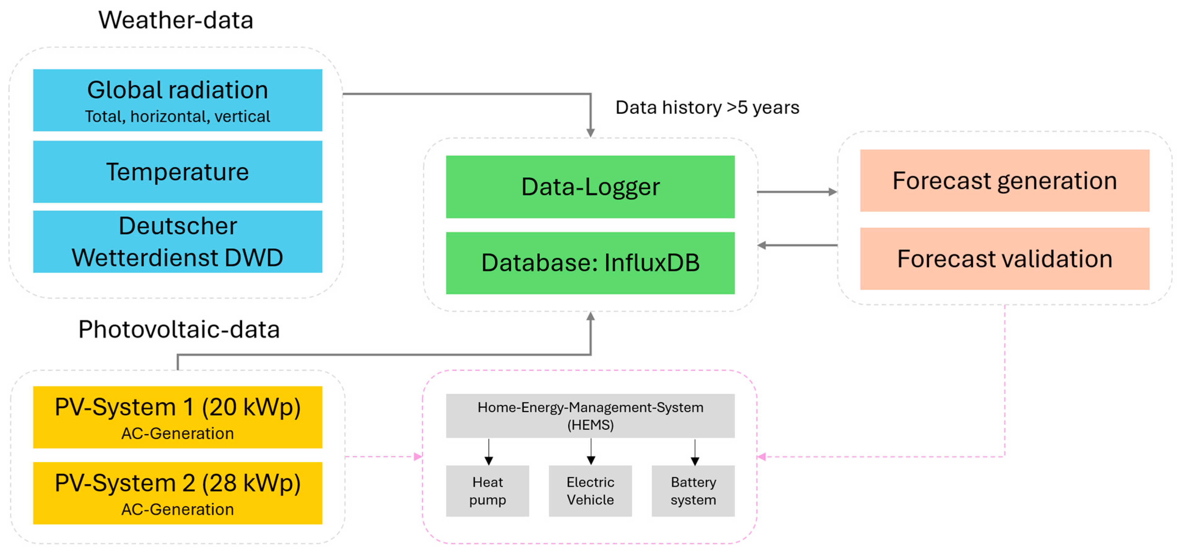
Overall, the building records approximately 1000 data points as time series. For this analysis, the collected data includes global solar radiation, temperature, and the AC production profiles of the two PV systems.

Additionally, data from Weather Station 7369 is utilised. The data is tracked by a data logger at a 60-s resolution and stored in an Influx database. A significant portion of the data has been historically recorded for over five years. The long-term goal is to use the PV surplus and forecast data to optimise the control of flexible loads in a CO₂₋ and cost-efficient manner. Figure 2 shows the functioning of the HEMS linked to data acquisition and forecasting.

3.1. Machine Learning Methods

3.1.1. Neural Networks

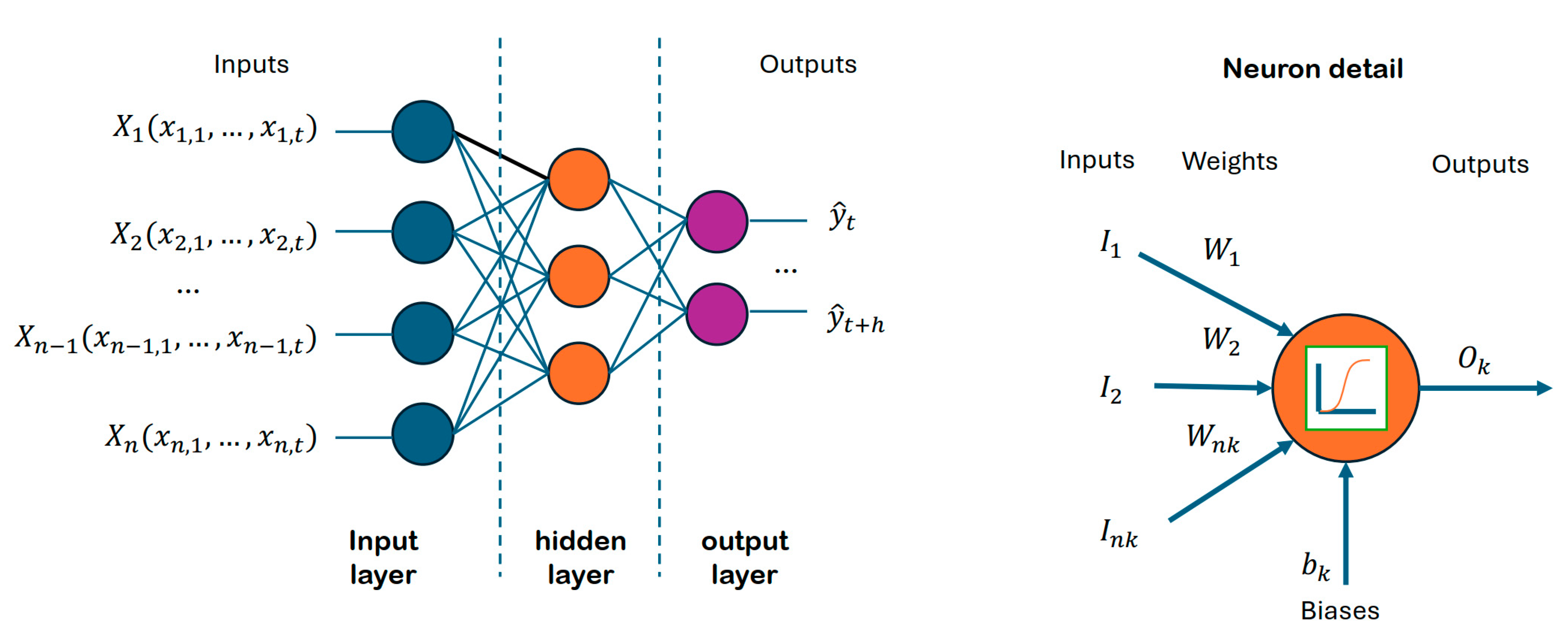
Neural networks are computational models composed of neurons, which are interconnected nodes organised in layers, that produce an output signal processing inputs received from other neurons or input data. The neurons are organised in layers: an input layer, where neurons are connected to the input variables, and an output layer, connected to output variables. All of them are interconnected through the neurons in the hidden layers. This structure can be seen in Figure 3.

There, $y_t$ represents the observed data and ${\widehat{y}}_{t+h}$ the h steps ahead predicted values. $X_n$ are time series variables related to the model, e.g., weather variables. The way the neurons are connected is through weighted links $W_i$ called axioms connected to inputs $I_i$. Every neuron k is connected to nk inputs that could be information from variables, or the outputs from other neurons. Additional biases $b_k$ permits more flexibility in the model. Inputs and biases are processed through an activation function $f$ to obtain an output $O_k$. The activation function introduces non-linearity properties to the network. The function can be either a linear activation, sigmoid, Tanh, or ReLU, among others, depending on the objective of the NN [14]. The output function related to each neuron can be stated as in (1).

$$O_k={\sum }_{i=1}^{nk}{W}_i{I}_i+b_k$$

(1)

One common type of neural network is the feedforward neural network, which consists of an input layer, one or more hidden layers, and an output layer. The input layer receives the initial data, such as images, text, or numerical values. Each neuron in the hidden layers applies a weighted sum of inputs and a nonlinear activation function, transforming the input data into a form suitable for the next layer. Finally, the output layer produces the network’s prediction or classification.

The global formulation of the neural network can be expressed as in (2).

$${\widehat{y}}_{t+1}=f(X_1,X_2,\dots ,X_n)$$

(2)

Training a neural network involves adjusting the weights of connections between neurons to minimise the difference between the network’s predictions and the actual targets. This is typically done using optimisation algorithms like gradient descent, combined with a loss function that quantifies the difference between predicted and actual values, measured using Mean Squared Error (MSE).

3.1.2. Least Squares Boosting Ensemble (LSBoost)

Ensemble methods are becoming more important every day in machine learning. The philosophy of working with these methods is to use apparently simple techniques that would not be expected to obtain great results and combine them so that the precision of their predictions increases considerably. Sets can be made using one of three different ways: bagging, boosting, and stacking. In our case, we have chosen to use the second.

Boosting leverages previous predictor errors to enhance future predictions. By amalgamating multiple weak base learners into a single strong learner, boosting markedly enhances model predictability. The process involves organising weak learners sequentially, allowing each learner to learn from its predecessor, thereby iteratively refining predictive models.

LSBoost algorithm [25] consists of sequentially building a series of regression trees, in which residuals of the previous trees are predicted through a loss function as in (3).

$$L\left(y_t,F_m\right)={\displaystyle \frac{{\left(y_t-F_m\right)}^2}{2}}$$

(3)

Being $F_m$ the regression tree on each stage and the first term $F_0\left(X\right)=y$. Each subsequent tree focuses on reducing the errors made by the previous trees, see Equation (4) and thereby gradually improving the overall prediction accuracy.

$$F\left(X,\left\{{{\rho }_m;\alpha }_m\right\}\right)={\sum }_{m=1}^M{\rho }_{m}h(X,{\alpha }_m)$$

(4)

With $M$ the maximum number of trees, and $h$ being a simple parametrized function of the observed data X using the parameters $\alpha$ and $\rho$. The final prediction is obtained by summing up the predictions from all the trees in the ensemble. An optimisation problem by minimising the errors is applied, and the numerical values of the parameters, as shown in (5), are obtained.

$$\left({\rho }_m,{\alpha }_m\right)=\mathrm{argmi}{\mathrm{n}}_{\rho ,\alpha }L(y_t,F_m)$$

(5)

This direct optimisation of the loss function makes LSBoost well-suited for regression problems, where the goal is to minimise the squared differences between predicted and observed values [26].

3.2. Novel Hybrid TBATS-ML Method

An exhaustive analysis of the time series reveals a deterministic component that traditional methodologies, such as exponential smoothing can predict. On this occasion, we have considered the use of state space models such as TBATS (Exponential smoothing state space model with Box-Cox transformation, ARMA errors, Trend and Seasonal components) [27]. A mathematical description of the TBATS models and all parameters can be found in the Appendix A at the end of the manuscript. In this article we considered two seasonal patterns: one for the daily seasonal cycle, and another for a yearly. The models to be adjusted were expressed as TBATS$(\omega ,\varphi ,p,q,\left\{24,k_{24}\right\},\left\{8760,k_{8760}\right\}$. The forecast library (version 8.20) of R software (version 4.4.1) has been used [27] for making the forecasts.

Once the TBATS state space prediction models have been obtained, this information from the deterministic part is used in an integrated way in A.I. models, similar to the process used in [28]. Within a neural network or ensemble regression model, the TBATS-adjusted variable is included in addition to a selected set of climatological variables from the DWD. New synthetic variables are added to this set to help the model in the prediction.

Finally, the model is trained by separating the training set into two subsets, one for fitting and one for validation of the model predictions. It is fitted by minimising the MSE (Mean Squared Error) and validated with the predictions made in the validation subset.

3.3. Accuracy Metrics

Metrics allow us to determine the model’s accuracy level in making predictions, all of which are based on prediction error. There are many metrics and no one metric can be considered the most suitable to perform the tasks. However, it is customary to use the MSE to fit prediction models, while others, such as the root mean square error (RMSE), as shown in (6), and the mean average percentage error (MAPE), are used to compare prediction accuracy and precision. In this case, the MAPE is discarded because it requires the values to be strictly positive, which is not the case.

$$RMSE=\sqrt{{\displaystyle \frac{{\left(y_t-{\tilde{y}}_t\right)}^2}{N}}}$$

(6)

where $N$ is the total number of observed values. The problem with RMSE is that it values the error absolutely, and comparing two stations of different capacities may be ineffective. Following [29], $NRMS{E}_{installed}$, which is defined in (7), will be used.

$$NRMS{E}_{installed}(\%)={\displaystyle \frac{\sqrt{\frac{{\left(y_t-{\tilde{y}}_t\right)}^2}{N}}}{P_{installed.peak}}}·100$$

(7)

4. Case Study: Prediction of Energy Production in PV Systems

The two solar panels located in the Feuchtwangen Campus at the Hochschule Ansbach are named PV-System1 (PV1), with a maximum peak production of 20 kW, and PV-System2 (PV2), with a maximum peak production of 30 kW. The data corresponds to the PV production from 2021 to March 2024, quarter-hourly measured. We reserved data from January 2024 to assess out-of-sample forecasts. The data was down-sampled for hourly measures to be synchronised with climate data obtained from DWD. 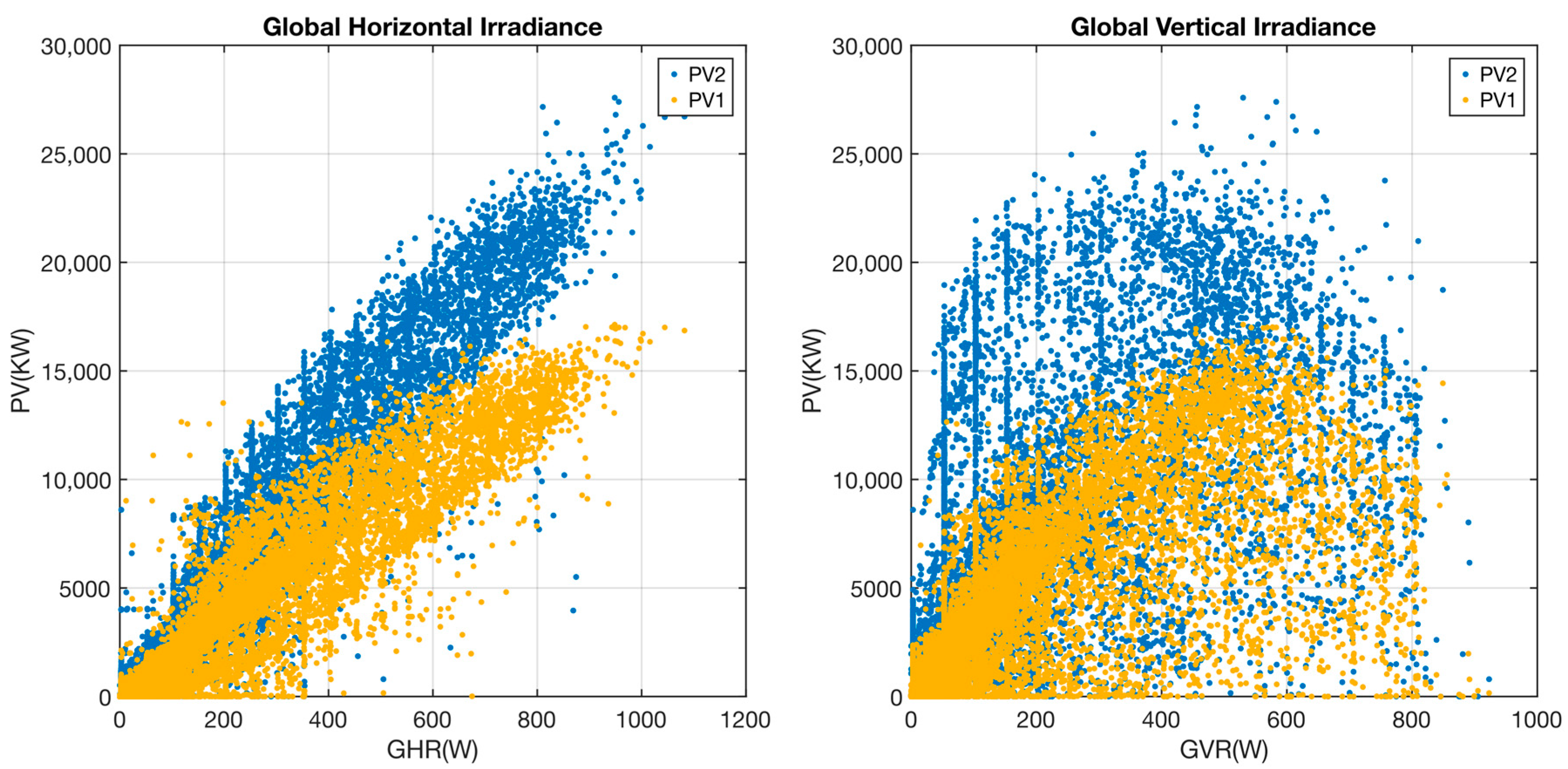Figure 4 shows the PV data for the period.

The figure shows the different behaviour of both PV installations. The orientation of the solar panels differs between both systems: 1 pure west orientation, 2 mixed south east orientation. Irradiation and energy production differ slightly between the systems (later peak and more outlies in the evening in system 1, ealier peak and more outliers in the morning) regardless of weather conditions. If we observe the behaviour of both installations with respect to the irradiance received (see Figure 5), we can see that there is a higher ratio for PV2 compared to PV1 for both Global Horizontal Irradiance (GHI) and Global Vertical Irradiance (GVI), which corroborates the situation described above.

Traditional methods of forecasting PV power from clear-sky radiation have limitations due to installation factors [30]. These methods often overlook localised atmospheric variations and installation-specific characteristics, such as panel orientation and shading effects. In addition, they do not account for dynamic weather patterns, resulting in inaccurate predictions. Advanced techniques incorporating site-specific data and machine learning are needed to improve forecast accuracy.

In any case, weather conditions are essential for solar PV production. Therefore, in order to carry out production forecasting, weather conditions must be taken into account. The climatological information used in this article has been obtained from the open database of the Deutsche Wetterdienst on its website https://opendata.dwd.de/ (accessed on 17 May 2024) [31].

4.1. Data Cleaning

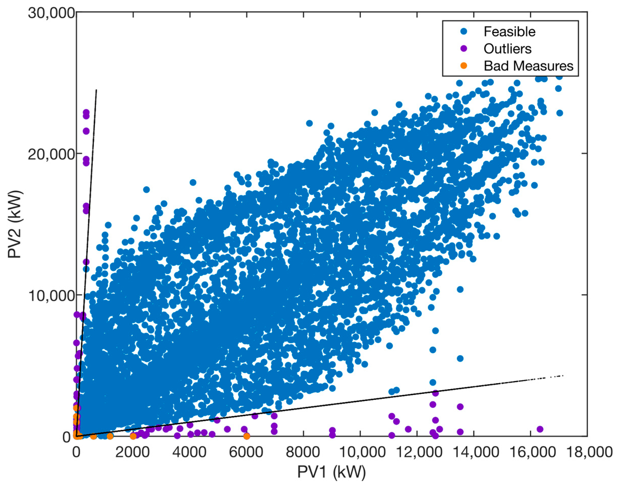
In any forecasting process, the forecaster must solve existing problems in the time series, either missing data or outliers. On this occasion, it is also necessary to deal with clearly erroneous measurement data, which are produced by errors provided by sensors. These are errors that can go unnoticed when training the models and introduce noise in the prediction models. Figure 6 reflects this situation, showing the values labelled as Feasible, Anomalous and mismeasurement. It can be seen how the data has been sectorized around the feasible region and the rest of the data to be corrected or eliminated.

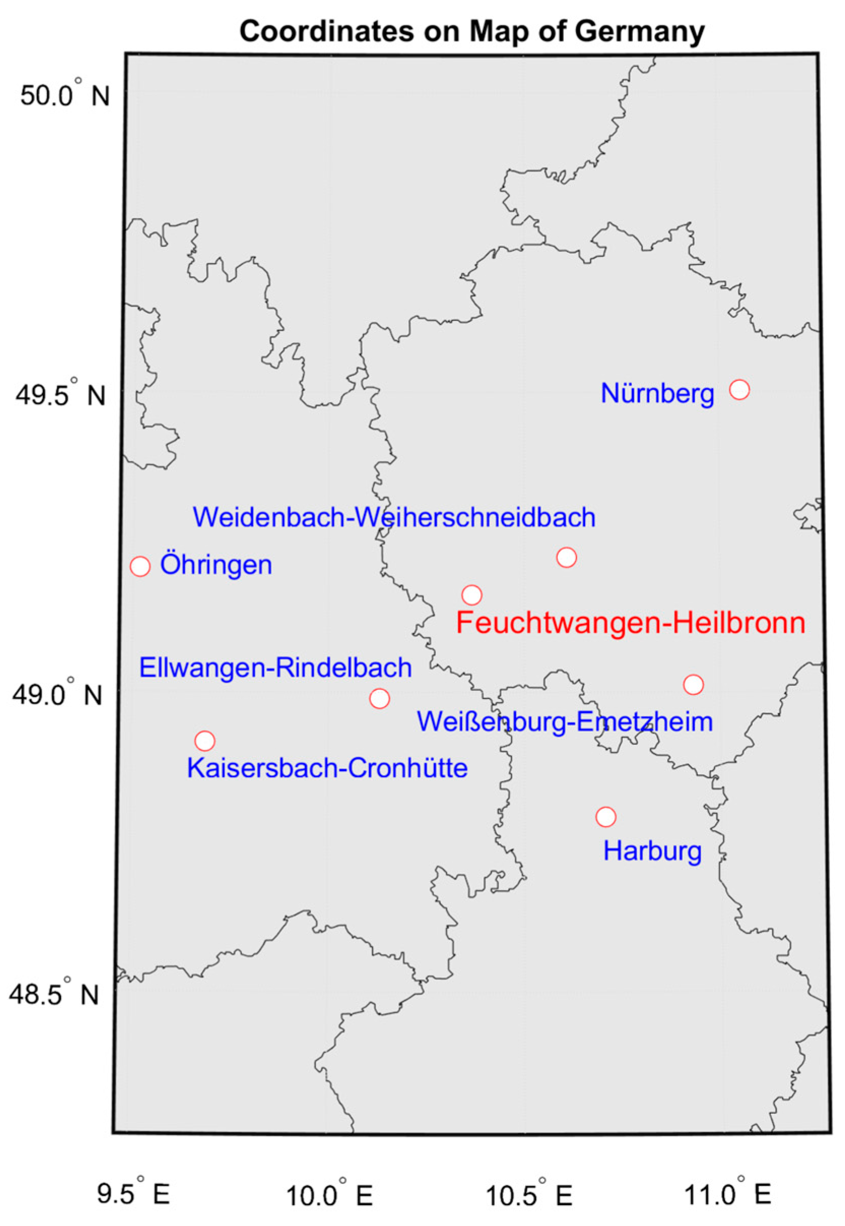
In the case of climatological variables, there is a similar situation with a large amount of missing data. In this case, we have resorted to generate regression models by means of A.I. using data provided by nearby weather stations that could provide reliable data for those moments of time. We followed filling procedures as explained in [32] but results were almost similar in all cases, so we decided to use MLP methods for this purpose. Figure 7 shows the stations from which data could be obtained.

Finally, after completing the series, we proceeded to reconstruct the PV1, PV2, GHI and GVI series. The result of the data cleaning is shown in the attached video. It includes a representation of the variables PV1, PV2, GHI and GVI over time, both in their original and repaired values.

4.2. Training and Forecasting

The data set worked on in this article covers the period from 1 January 2022, to February 2024. These are the data collected by the Feuchtwangen Campus facility. This set has been divided into three subsets: The training set, which includes the first period from January 2022 until 30 September 2023. A second set for in-sample validation, until 31 December 2023. Finally, the out-of-sample test set until March 2024.

The training of the models and their validation has been carried out using the facility’s own variables, in addition to the current climatological data provided by the DWD. In addition, synthetic variables that help the model to make predictions are included. These variables are listed in

Table 1. Synthetic variables created for the models.

Name	Description	Values
sun	Sun	Binary
PV1/PV2 d24	Power measurements generated in PV1/PV2 delayed 24 h	Real
Hour/month	Day/month of the year	Integer 1–24/1–12
DayOfYear	Consecutive day within the year	Integer 1–366
WeekOfYear	Calendar week within the year	Integer 1–53
TBATS	Data modeled using TBATS for the structural part of the model	Real

.

Subsequently, the models have been trained and the variables to be used in the predictions have been selected. The procedure includes a selection by Minimum Redundancy Maximum Relevance (MRMR) Algorithm [33] and F tests [34].

Due to the different characteristics of each installation, the variables used in each case do not coincide. This will be analysed later in the discussion of the results. Nevertheless, the procedure followed to perform the training and predictions with both facilities is the same.

In the case of prediction, two different prediction strategies have been analysed: In the first, current climatological data are used and forward prediction is performed using that observed base; in the second option, predicted climatological data provided by the DWD are used.

5. Results

The models have been analysed according to two strategies. The first one consists of using the current data, with which the models are trained, and from them make predictions of the energy production always based on the past. This makes sense if we take into account the inertia of time and the fact that day-to-day variations are not large. The other strategy is to make forecasts using the current production data, but using the climatological values predicted by the DWD. This delegates the responsibility of the climatology prediction to the DWD, although it depends on it, and it is necessary to know it to be able to make our predictions.

The differences between both strategies are not very dissimilar, however, this second strategy seems to provide better results independently of the installation and the models used, so it has been chosen to continue with it. The results are shown separately for each facility to facilitate reading comprehension.

Additionally, alternative methodologies not listed in the article were tested during the course of this study. They are not described in detail in the manuscript, as their performance was found to be inefficient and they were discarded. Comparisons with traditional prediction methods were also ruled out, primarily due to the impracticality of applying irradiance-based models in the context of our experimental setup. Thus, this work focuses exclusively on the approaches that demonstrated promising outcomes, avoiding those with unsatisfactory results.

5.1. PV System 1

The first step in the prediction was the estimation of the TBATS state space model using the forecast library. The model obtained was TBATS(1, {2,2}, -, {<24,6>, <8760,7>}). As explained, two seasonalities have been considered: an intraday and an interannual one.

Starting with all the variables offered by the DWD, an initial screening has been carried out by selecting those variables whose influence on the model is significant, both with the application of the F-Test method and the MRBR method. The use of more variables does not imply an increase in the precision of the model. Once the models have been adjusted, by means of an iterative procedure and aided by the SHAPLEY curves, the number of variables is reduced. Tests using principal component analysis have not been effective, so their use has been discarded. The strategy selected for this installation has been the use of the predictions provided by DWD.

The model has been fitted and 24-h forward predictions have been made on both the validation set and the out-of-sample test set.

Table 2. Comparison of tested models for PV1 installation.

Model	Validation RMSE	Forecasting RMSE	Forecasting NRMSE
Ensemble (LSBoost, min.leaf size:1, L.R. 0.042)	622	445	2.25%
Neural Network (Shallow, 1 Layer Size: 24)	699	621	3.11%
Tree (Non surrogate)	688	626	3.13%

shows a comparison of the models tested and the results obtained in their predictions.

Clearly, the Ensemble method outperformed the others in terms on accuracy, and has been selected for new forecasts. According to this model,

Table 3. Main climate variables used in the forecasts.

Name	Description	Values
V_VV	visibility	m
TT, TT_TU	air temperature	°C
RF	relative humidity	%
FF	Wind speed	°C
V_TEXXX	Soil temperature in XXX cm depth	°C

shows the selected climatological variables included. The table shows the variables and the description of the data obtained from DWD.

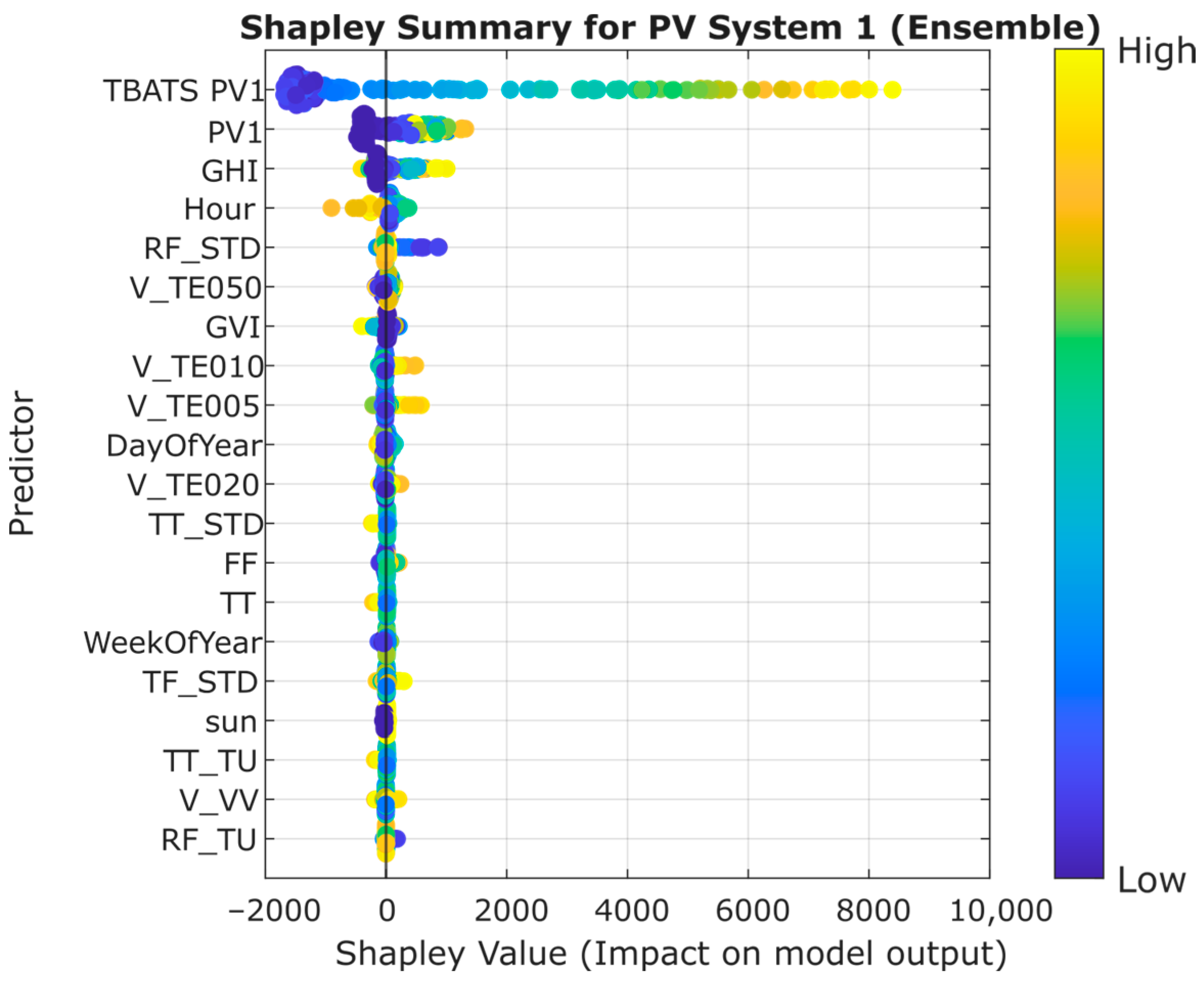
The SHAPLEY graph shown in Figure 8 shows the importance of each of the variables included in the selected model. In this case, soil temperature is observed to be influential in the model. Due to the inherent characteristics of the models, as illustrated in the SHAPLEY plots, the PV1 model demonstrates reduced flexibility in responding to anomalous meteorological conditions.

5.2. PV System 2

Following the same procedure as the previous case, the TBATS model obtained for the structural part of the model is: TBATS(1, {2,2}, -, {<24,6>, <8760,5>}). Finally,

Table 4. Comparison of tested models for PV2 installation.

Model	Validation RMSE	Forecasting RMSE	Forecasting NRMSE
Ensemble (LSBoost, min.leaf size:1, L.R. 0.042)	1358	987	3.52%
Neural Network (3 Layers of Sizes 4,1 and 9, Std.)	1226	917	3.28%
Tree (Non Surrogate)	1494	1097	3.92%

shows the values of the metrics obtained using each of the models. On this occasion, the neural network model outperforms the ensemble model in both validation and out-of-sample test predictions.

The NRMSE values are around 3.5% while for the previous case they were around 3%. This loss of precision in the predictions is mainly due to the fact that the structural component has less significance and that the climatological variables generally have greater variability in the prediction.

The climatological variables included in the selected model for PV-System 2 are shown in

Table 5. Climate variables used in the forecasts.

Name	Description	Values
V_N	visibility	1–8
TT_TU,TT_STD	air temperature	°C
RF_XXX	relative humidity	%
V_TEXXX	Soil temperature in XXX cm depth	°C
V_S1_Ns	Height of clouds 1st layer	m

. As can be seen, the variables do not coincide with those in Table 3, corroborating in part the different characteristics of both installations. There is a lower presence of variables related to temperature and a higher presence of variables related to cloudiness.

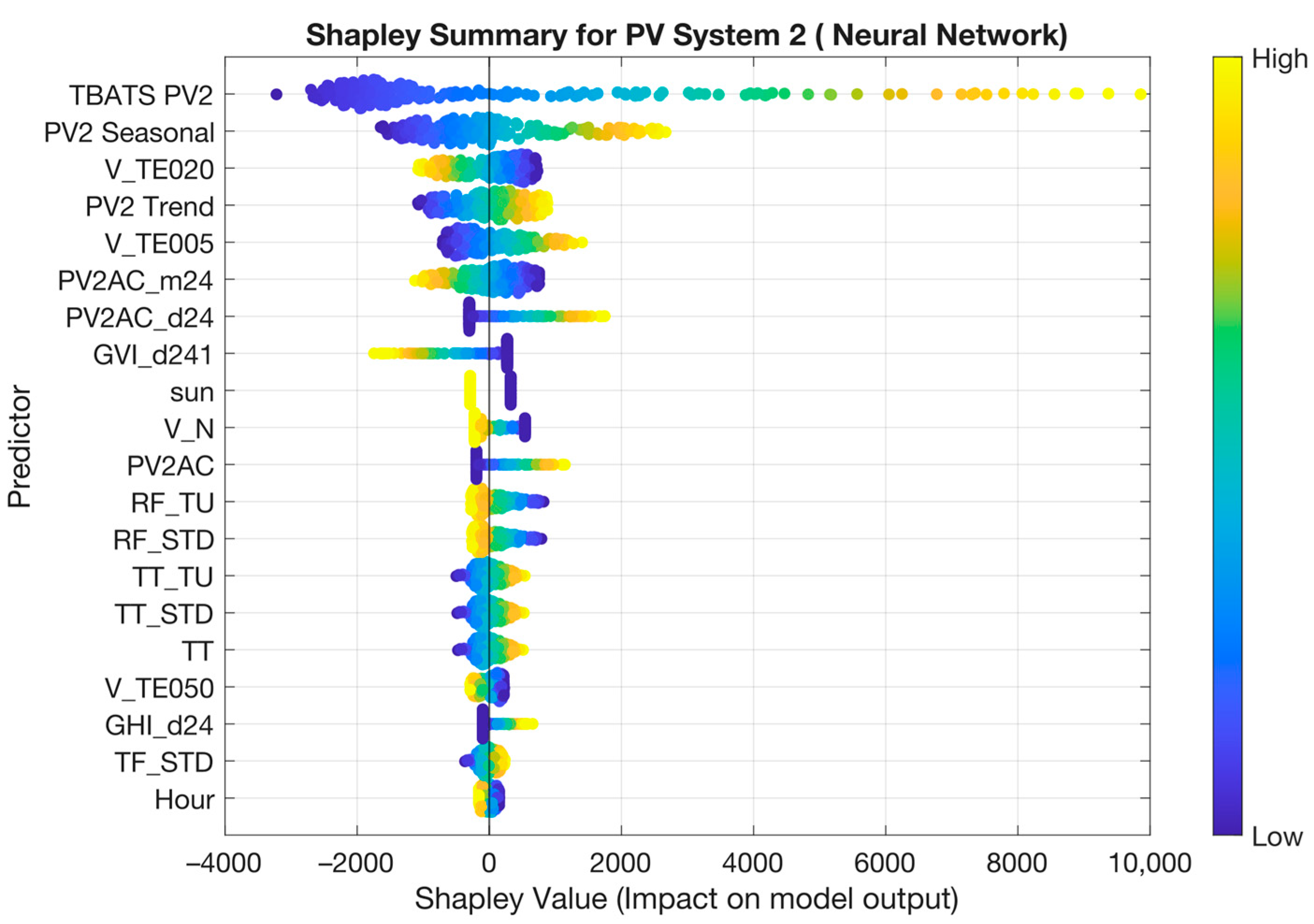
Figure 9 shows the SHAPLEY diagram in swarm format for the model chosen for the PV 2 installation. The climatological components become more important and the seasonality is more pronounced.

5.3. Discussion

The use of TBATS in the model allows for more accurate predictions, as shown by the nMAPEs of PV1 and PV2. In the PV-System 1 installation, this variable is the main variable and by far more important than the rest. In PV-System 2, the influence of TBATS is minor, although it is the main predictor. It was an expected result due to the fact that the panels of both systems have different solar alignments. It can be observed how in the second installation, the model is more affected by the climatological variables, especially those related to ground and air temperature.

This is mainly due to the orientation of the modules. For system 1 with a pure west orientation the TBATS PV 1 dominates in Figure 8 while system 2 with a mixed south east orientation is more affected by climatology.

In order to establish whether the predictions are within an acceptable level, they have been compared with the literature. Thus, for example, in [14] several papers with nRMSE around 9.5% [35], 5.29% [36] or 1.33% [37] are mentioned. The problem is that there is no single criterion for their calculation. Thus, in [36], the calculation for 24-h-ahead forecast accuracy is normalised over the range of the prediction, while in [35], it is calculated as we have done, using the installed capacity. In any case, the values obtained indicate that the predictions are accurate.

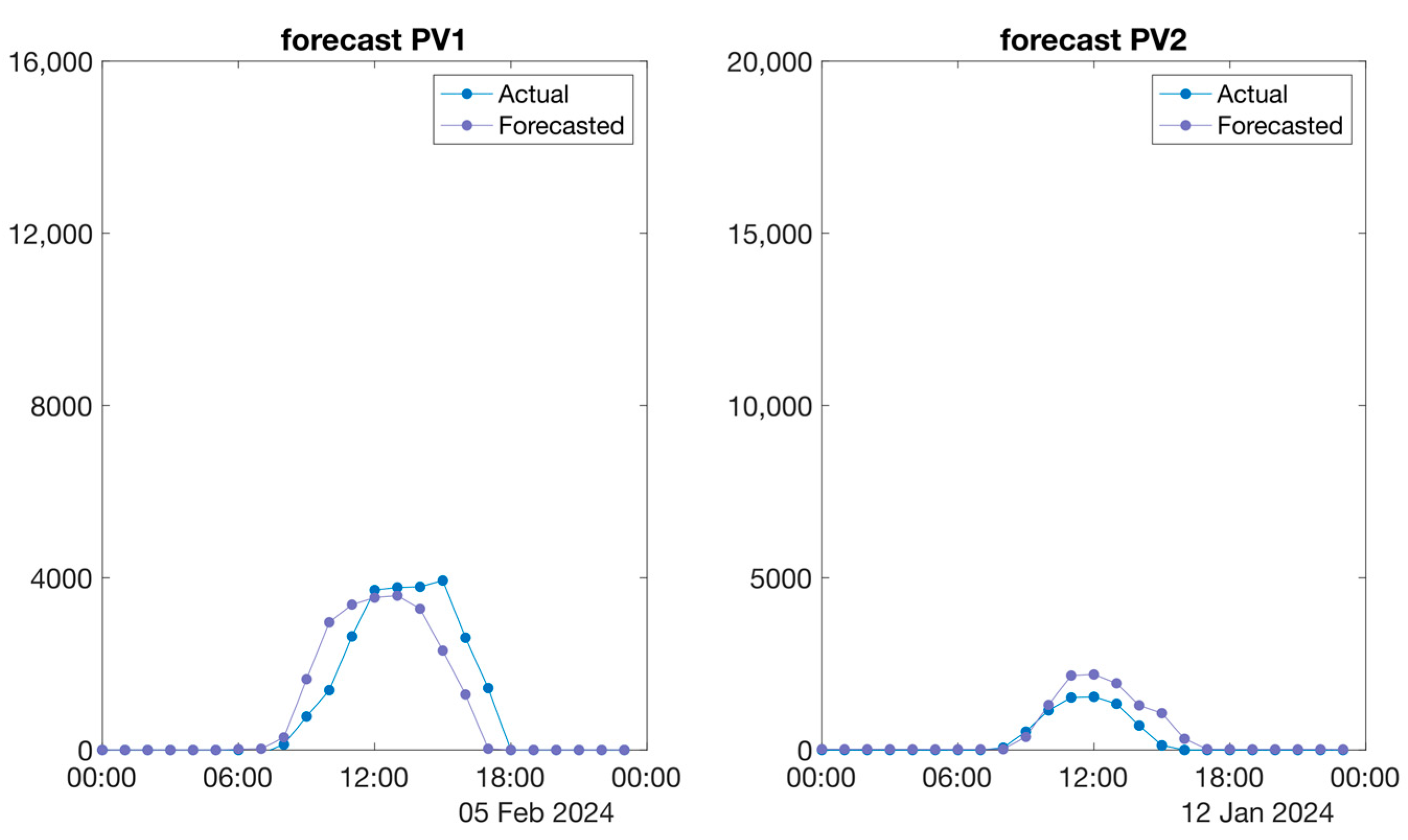
Finally, and for better understanding, we show in Figure 10 the comparison of the predicted values against the actual values in a typical day.

6. Conclusions

In this paper, machine learning methods have been used to predict the PV generation of the Campus Feuchtwangen with a 48 kWp system. The layout of the strings and the orientation of the panels do not allow the simplified use of traditional prediction methods, which are generally based on the use of the orientation angle and the location of the installation.

Therefore, past observed data and the use of climatological data obtained from the DWD have been used to predict both energy production and irradiance, presenting a hybrid prediction model based on time series and with the help of artificial intelligence. The new method is based on the introduction of TBATS state space models that, through the use of AI with the help of climatological variables, allow predictions to be made.

The results obtained indicate that the prediction accuracy is around 3% in nMAPE, which confirms that the incorporation of TBATS into the model improves its performance. Depending on the setup, different methodologies were required. Thus, for the PV1 installation, ensemble models with LSBoost have provided the best results, with nMAPE of 2.25%, while for PV2 systems neural networks have been used with an accuracy of 3.28%. The fact that system 1 is only west-facing and system 2 has an east, south and west aspect must be taken into account.

The accuracy of photovoltaic power predictions plays a fundamental role in supporting effective energy planning and operational decision-making. However, it is equally important to account for the uncertainty inherent in such predictive models. Providing information on the degree of uncertainty is necessary to support informed decision-making, particularly in applications where reliability and performance forecasting are critical. For this reason, future predictive outputs will be accompanied by appropriate indicators of model confidence or variability.

However, the results obtained are only framed for the period considered and for one building (Campus Feuchtwangen). While the results obtained are specific to the configuration analysed in this study, the methodology developed is extensible to other photovoltaic installations, especially those featuring mixed orientations. Furthermore, this approach can be extended to systems in which conventional forecasting methods fail to deliver satisfactory outcomes. The generalizability of the proposed model lies in its capacity to adapt to diverse spatial configurations and irradiance profiles, thereby offering a robust alternative for performance forecasting in complex or non-standard scenarios.

In future works we will try to go deeper into the physical elements of the facility to increase the accuracy of the predictions. Future research will also focus on developing and integrating uncertainty quantification methods to improve the reliability and usability of forecasting tools in practical energy management contexts.