Article

A Simplified Model Validation for the Energy Assessment of Opaque Adaptive Façades with Variable Thermal Resistance

by
Ismael Palacios Mackay
1,
Laura Marín-Restrepo
1 and
Alexis Pérez-Fargallo
2,*
1
Department of Building Science, Universidad del Bío-Bío, Concepción PC 4051381, Chile
2
Escuela de Arquitectura, Facultad de Arquitectura, Arte y Diseño, Universidad San Sebastián, Concepcion PC 4081339, Chile
*
Author to whom correspondence should be addressed.
Energies 2025, 18(11), 2682; https://doi.org/10.3390/en18112682
Submission received: 20 March 2025 / Revised: 11 May 2025 / Accepted: 14 May 2025 / Published: 22 May 2025
(This article belongs to the Special Issue Advanced Building Materials for Energy Saving—2nd Edition)

Abstract

:
Adaptive façades, also known as climate-adaptive building shells (CABSs), could make a significant contribution towards reducing the energy consumption of buildings and their environmental impacts. There is extensive research on glazed adaptive façades, mainly due to the available technology for glass materials. The technological development of opaque adaptive façades has focused on variable-thermal-resistance envelopes, and the simulation of this type of façade is a challenging task that has not been thoroughly studied. The aim of this study was to configure and validate a simplified office model that could be used for simulating an adaptive façade with variable thermal resistance via adaptive insulation thickness in its opaque part. Software-to-software model comparison based on the results of an EnergyPlus Building Energy Simulation Test 900 (BesTest 900)-validated model was used. Cooling and heating annual energy demand (kWh), peak cooling and heating (kW), and maximum, minimum, and average annual hourly zone temperature variables were compared for both the Adaptive and non-adaptive validated model. An Adaptive EnergyPlus model based on the BesTest 900 model, which uses the EnergyPlus SurfaceControl:MovableInsulation class list, was successfully validated and could be used for studying office buildings with a variable-thermal-resistance adaptive façade wall configuration, equivalent to a heavyweight mass wall construction with an External Insulation Finishing System (EIFS). An example of the Adaptive model in the Denver location is included in this paper. Annual savings of up to 26% in total energy demand (heating + cooling) was achieved and could reach up to 54% when electro-chromic (EC) glass commanded by a rule-based algorithm was added to the glazed part of the variable-thermal-resistance adaptive façade.

1. Introduction

Climate change and the urgent need to reduce energy demand in buildings, of which 36% of the energy consumption is related to greenhouse gas emissions [1], accounting for approximately 40% of the total energy consumption in the European Union (EU), have triggered research that has the goal of achieving nearly-zero-energy buildings and net-zero-energy buildings (nZEB and/or NZEB) for new constructions [2,3,4,5,6]. On the other hand, in Chile, buildings account for 22% of the country’s energy consumption [7], and a national energy efficiency plan was established for the 2022–2026 period to immediately trigger policies and construction standards to reduce the energy demand towards achieving the NZEB target by 2050.
The principle of energy conservation inside buildings, based on minimizing heat losses and maximizing heat gains, has been one of the paradigms for building envelope design [8,9]. The design’s goal is to select a thermal resistance value for the envelope’s insulation that minimizes the annual total energy demand (heating + cooling). However, the chosen value is not the daily or even monthly optimum value but is rather a compromising value for the entire year; it is the equivalent of making a design for an average situation [10,11,12]. Energy conservation principles have been derived for envelope designs that select, among other parameters, the same thermal resistance value for the whole envelope and for the whole year. The paradigm shift needed to achieve the nZEB goal consists of switching from static façades to adaptive façades for building envelope designs, where the envelope’s thermo-physical and/or thermo-optical characteristics could change and adapt throughout the year due to changing outdoor and/or indoor conditions, in order to improve the building energy performance [13,14,15,16,17].
CABSs are capable of changing some of their functions, characteristics, or behaviors over time in response to changes in environmental conditions and user requirements in order to improve a building’s performance while maintaining human comfort inside the building [18,19]. “Intelligent” CABSs are capable of changing their behavior via an external (extrinsic) control signal driven by an algorithm or control logic that “decides” when and how the façade should change its characteristics in response to changing conditions [9,20] in order to minimize energy demand and maintain a certain degree of comfort.
Adaptive façades can be implemented in both the glazed and opaque parts of a building envelope [9,20,21]. In recent years, several adaptive façade technologies have been developed for the glazed parts, such as motorized blinds, window frames, and (EC) glazing for solar shading, among others [22,23,24,25,26,27]. However, technologies based on variable thermal resistance for the opaque part of façades are still under development [10,12,28], which limits the availability of experimental data. Consequently, building performance assessments for adaptive insulation are scarce and they are mostly theoretical and based on building performance simulation (BPS).
Considering that the available BPS software can be used to model and simulate the glazed sections of adaptive façades, several studies have been conducted using BPS software for such adaptive façades [29], with different technologies being examined, including vertical, horizontal, baffle, and integrated louver shading [30], perforated curved louvers [26], movable window insulation and window frames [31,32,33], and adaptive materials such as EC glass [34,35], photovoltachromic glass [36], and thermochromic glass [37,38]. However, the evaluation of adaptive insulation based on variable thermal resistance for the opaque part of façades is complex. This is due to the lack of building simulation models for specific technologies among other limitations of BPS software which include the user interface, solution routines, control strategies, occupant influence, and domain integration [39,40]. Specifically, for the variable-thermal-resistance simulation of opaque façades, there are limitations in terms of the capability of BPS software to model the variable thermal resistance and to explicitly indicate the border conditions from the previous time step, which are the initial conditions for the next time step, specifically in systems that are dominated by the building’s time constant.
Moreover, there has not been any comparison between experimental measurements and simulated data for a specific adaptive insulation system [12,41]. By using the EnergyPlus “SurfaceControl:MovableInsulation” class list [42], an Adaptive insulation model could be defined with the ability to change the insulation thickness during run time to achieve adaptation. This is in contrast with a non-adaptive model, where insulation thickness must be changed manually (via code modification) before a new simulation run and cannot be changed during run time.
However, it is desirable to have a validated model to simulate the opaque section of adaptive façades that takes into account not only the temperatures at the interface between the insulation layer and the concrete and along the concrete layer [39] but also other variables of interest for building performance simulation, such as annual heating and cooling energy demand, peak heating, peak cooling, and indoor temperatures (maximum, minimum, and average) throughout the year-long period of study.
The objective of this research was to configure and validate a simplified office model based on the BesTest 900 and BesTest 900 Free Floating (FF) models, as specified in the ANSI/ASHRAE Standard 140-2011. This could be used to simulate an adaptive façade with variable thermal resistance via adaptive insulation thickness in its opaque section. To carry this out, a model was defined, and then, using the EnergyPlus “SurfaceControl:MovableInsulation” class list within the model, it was validated.

2. Materials and Methods

The model subjected to validation in this study was an “Adaptive” model based on a modified version of the BesTest 900 model [43]. It was coded and simulated in EnergyPlus software version 9.5.0. using the Windows 10 operating system environment and compared to a “Static” model that was used as a reference. The study site was in the Stapleton neighborhood in Denver, Colorado, USA, as indicated in the BesTest 900 specifications, fully described in Section 2.1. The “Static” and “Adaptive” versions, which are modified models of the original BesTest 900, are described in Section 2.2 and their EnergyPlus code differences are fully detailed in Appendix A.
The validation procedure of the “Adaptive” model presented in Section 2.3 was based on a software-to-software comparison [44] with the “Static” model that was previously validated for BesTest 900 and BesTest 900FF. For this validation study, the independent variable was the thermal resistance of the walls, which was modified by changing the insulation thickness, as explained in Section 2.2. The dependent variables were cooling annual energy demand (kWh), heating annual energy demand (kWh), peak heating (W) and peak cooling (W) for BesTest 900, and maximum annual hourly zone temperature (°C), minimum annual hourly zone temperature (°C), and average annual hourly zone temperature (°C) for BesTest 900FF. These dependent variables were the results of a year-long simulation of the models with the parameters, site, climate, and definitions of BesTest 900 indicated in Section 2.1. It should be noted that BesTest 900FF is a Free-Floating Temperature Test for BesTest900, and the construction model and simulation parameters are the same as those for BesTest 900 except that there is no mechanical heating or cooling system [43].

2.1. BesTest 900

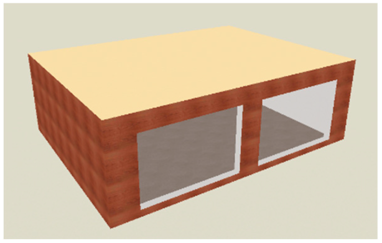
The basic testing building for BesTest 900 is shown in Figure 1. It is a rectangular, single-zone structure (8 m wide × 6 m long × 2.7 m high) with no interior partitions and 12 m2 of south-facing windows. It is located in the Stapleton neighborhood in Denver, Colorado, USA, and is one of the simplified models proposed by the ANSI/ASHRAE Standard 140-2011 [43]. The climate is characterized as cold, with clear winters/hot dry summers and an average number of annual heating degree days = 2756, considering a base temperature of 15.5 °C and data from the past 5 years. The BesTest 900 model specifications are shown in Table 1 and Table 2.
The BesTest 900 description of the heating and cooling systems, thermostat setpoints, and other parameters is the following:
  • Infiltration: 0.5 air change/hour.
  • Internal Load: 200 W continuous, 60% radiative, 40% convective, 100% sensible.
  • Mechanical System: 100% convective air system, 100% efficiency with no duct losses and no capacity limitation, no latent heat extraction, non-proportional-type dual-setpoint thermostat with deadband, heating < 20 °C, cooling > 27 °C.
  • Soil Temperature: 10 °C continuous.

2.2. Static and Adaptive Models

2.2.1. Static Model

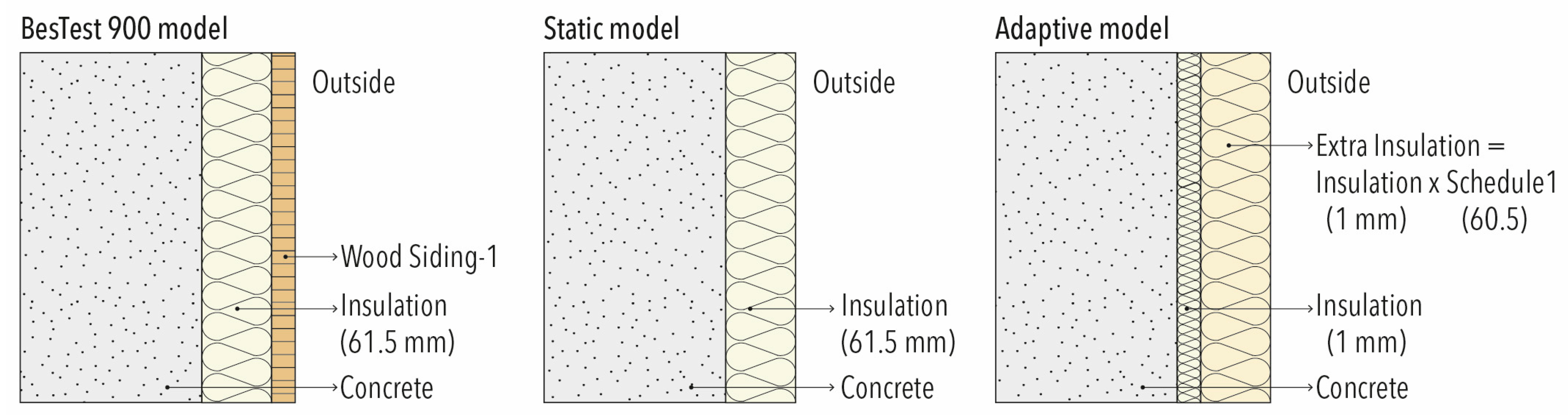
The model used as a reference for this study was the same BesTest 900 model, except for the “Wood Siding-1” shell, which was removed. This model variation is called “Static”, and the wall configuration is shown in Figure 2. The external layer of the Static model is the insulation; thus, this modified model is similar to a heavyweight-mass wall with an EIFS. For this study, the model variation is called the “Static” model because, in this model, the thermal resistance of its walls is fixed. The thermal resistance also depends on the amount and type of insulation as well as the materials included in the layers specified in the material, construction, and building surface of these EnergyPlus objects, aspects that could not be changed during run time. The Static model is used as the reference model and is taken from the original BesTest900 model that was validated using the software-to-software comparison methodology described by the ANSI/ASHRAE Standard 140-2011 (BESTEST) [43,44]. The results of this Static model are consistent and logically coherent as the only difference with the original BesTest 900 is the external Wood Siding shell that was removed from the BesTest900 original model to set up the Static model.

2.2.2. Adaptive Model

The “Adaptive” model shown in Figure 2 is an EnergyPlus model where the thermal resistance can be modified by changing the amount of extra insulation and during run time, by adjusting the “Schedule1” multiplier. The rest of the Adaptive model definitions are kept unchanged compared to those in the Static model.
The Adaptive model of Figure 2 is an example where the total insulation is equal to 61.5 mm. If the Schedule1 multiplier is changed, different total insulations can be achieved.
The Adaptive model was obtained by modifying the Static model using EnergyPlus code. The EnergyPlus “SurfaceControl:MovableInsulation” class list was used to add the ability to change the extra insulation added to the Static EnergyPlus model, allowing the wall’s thermal resistance in the model to be adjusted during run time to achieve adaptation in response to climate and/or interior occupancy changes within the study period.
The EnergyPlus “SurfaceControl:MovableInsulation” class list allows the user to specify an additional amount of insulation on the inside, outside, or both surfaces of a wall by adding the definition of the multiplier Schedule1 (see example in Figure 2). The actual insulation of the movable insulation that is added is equal to the insulation of the material layer times the current value in the movable insulation schedule [45].
The total insulation of the Adaptive model (see example in Figure 2) is calculated by adding the extra insulation that comes from multiplying the Schedule1 equal to 60.5 (example in Figure 2) by the insulation of the material layer (1 mm):
Final insulation thickness = 1 mm + 1 mm × 60.5 = 61.5 mm.
The example in Figure 2 shows that the Adaptive model is equivalent to the Static model, where the insulation thickness definition in the material layer is 61.5 mm.
The Adaptive model’s requirement is to achieve multiple insulation thicknesses to provide a variable-thermal-resistance model. For instance, if it is desirable for the Adaptive model to achieve a total insulation thickness of 30 mm, Schedule1 should be equal to 29 (1 mm + 1 mm × 29 = 30 mm); if it is desirable to achieve a total insulation thickness of 100 mm, Schedule1 should be equal to 99 (1 mm + 1 mm × 99 = 100 mm).
A detailed comparison of the EnergyPlus code differences for the Static and Adaptive models is presented in Appendix A.

2.2.3. Criteria for Selecting Thermal Resistances for Adaptive Model Validation

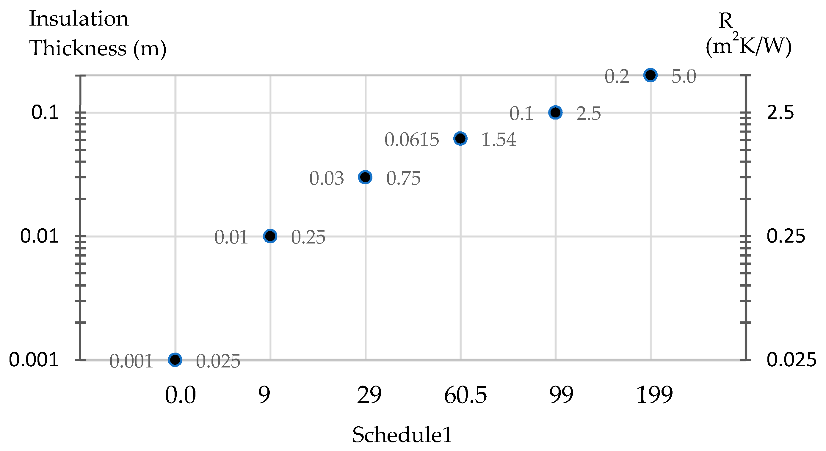
For this study, it is assumed that variable-thermal-resistance technology similar to that described in [46] is available and can reach up to 5.0 (m2 K/W). From the table defined by Palacios and Bobadilla [47] for an adaptive façade study, the thermal resistances that resulted in the most significant energy reduction were chosen for validation in this study. The BesTest900 thermal resistance used in the ANSI/ASHRAE Standard 140-2011 (BESTEST) is 61.5 mm, so this value was also included in the set. Considering the aforementioned study, the insulation thicknesses of 1 mm, 10 mm, 30 mm, 61.5 mm, 100 mm, and 200 mm were used as the chosen set to compare the simulation results of the Static model with those of the Adaptive model. It should be mentioned that BesTest 900 and 900FF use foam insulation. The insulation thickness and its thermal resistance value for the chosen set, considering a foam insulation lambda value of 0.040 (W/mK), are shown in Figure 3.
The possible insulation thicknesses for the Adaptive model range from a 1 mm total insulation thickness when no extra insulation is added (Schedule1 = 0.0) to 200 mm of total insulation, which is achieved when 199 mm of insulation is added (Schedule1 = 199).

2.3. Model Validation Procedure

2.3.1. Static Model Validation

The BesTest 900 and BesTest 900FF EnergyPlus original code was provided by EnergyPlus in version 8.1.0 and was converted to EnergyPlus version 9.5.0 using the IDFVersionUpdater provided by the EnergyPlus software. This conversion was necessary because at the time of this study, the original EnergyPlus BesTest 900 and BesTest 900FF code was only available for EnergyPlus version 8.1.0., and the validation was performed using EnergyPlus version 9.5.0. After the conversion described above, to obtain the Static EnergyPlus model using BesTest900 EnergyPlus version 9.5.0, the “Wood Siding” from the BesTest900 model construction definition was removed.
First Validation (Static Model Validation) Procedure:
The software conversion was verified by comparing the dependent variable results provided by EnergyPlus for the original code in version 8.1.0, with the EnergyPlus 9.5.0 converted code results, by using the software-to-software comparative test criteria described by the ANSI/ASHRAE Standard 140-2011 (BESTEST) [43,44].

2.3.2. Adaptive Model Validation

The results comparison between the Static (validated) and Adaptive models’ results was performed using the following procedure:
Second Validation (Adaptive Model Validation) Procedure:
  • Select one of the insulation thicknesses from the set detailed in Section 2.2.3 (1 mm, 10 mm, 30 mm, 61.5 mm, 100 mm, or 200 mm).
  • Adjust the Static model construction definition to achieve the chosen insulation.
  • In the Adaptive model, set the Schedule1 parameter to achieve the same total insulation chosen for the Static model. For example, if a 100 mm insulation thickness was chosen in step 1, then Schedule1 should be set to 99 to achieve a total insulation of 100 mm as explained in Section 2.2.2. (Figure 2).
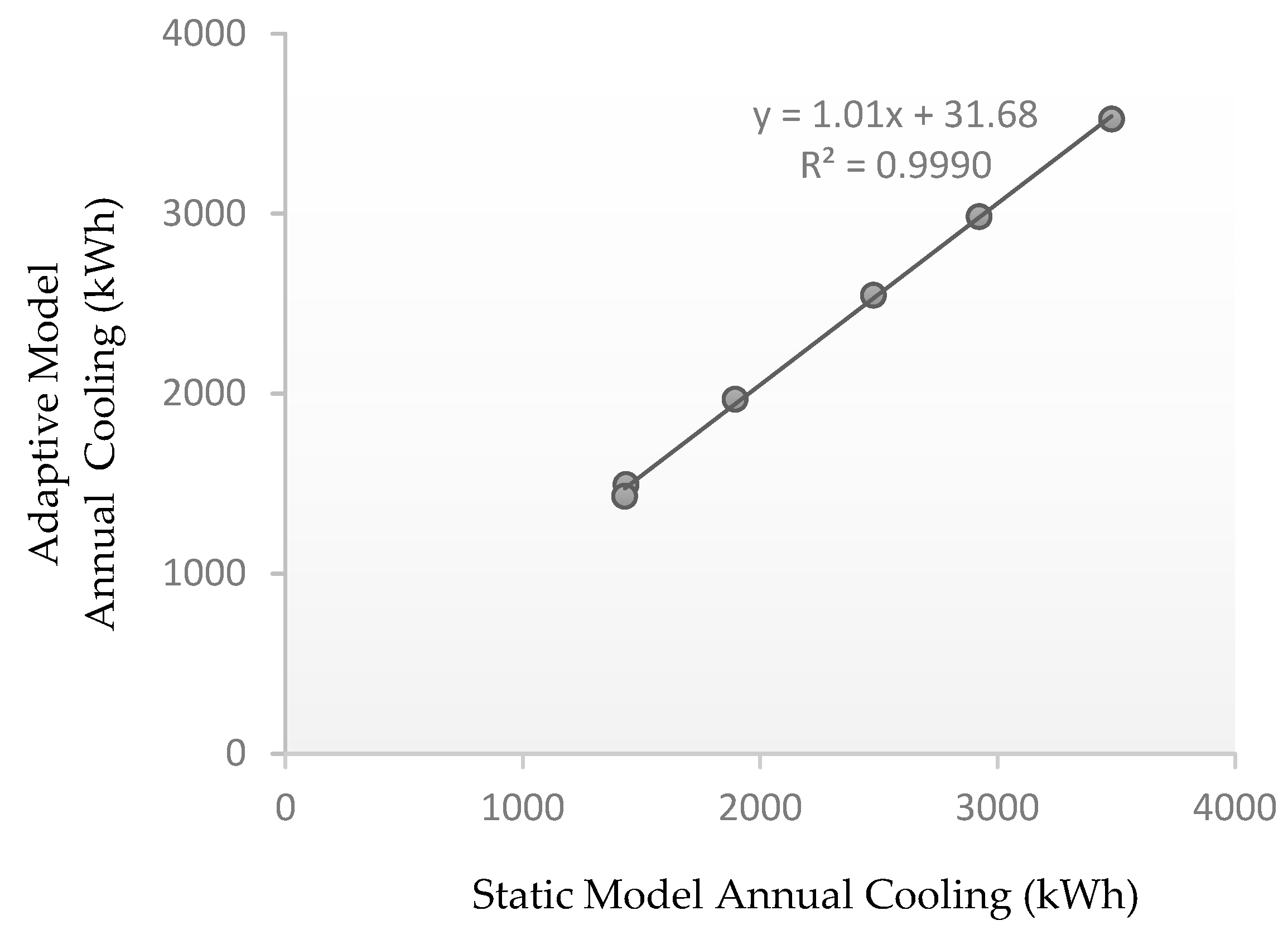
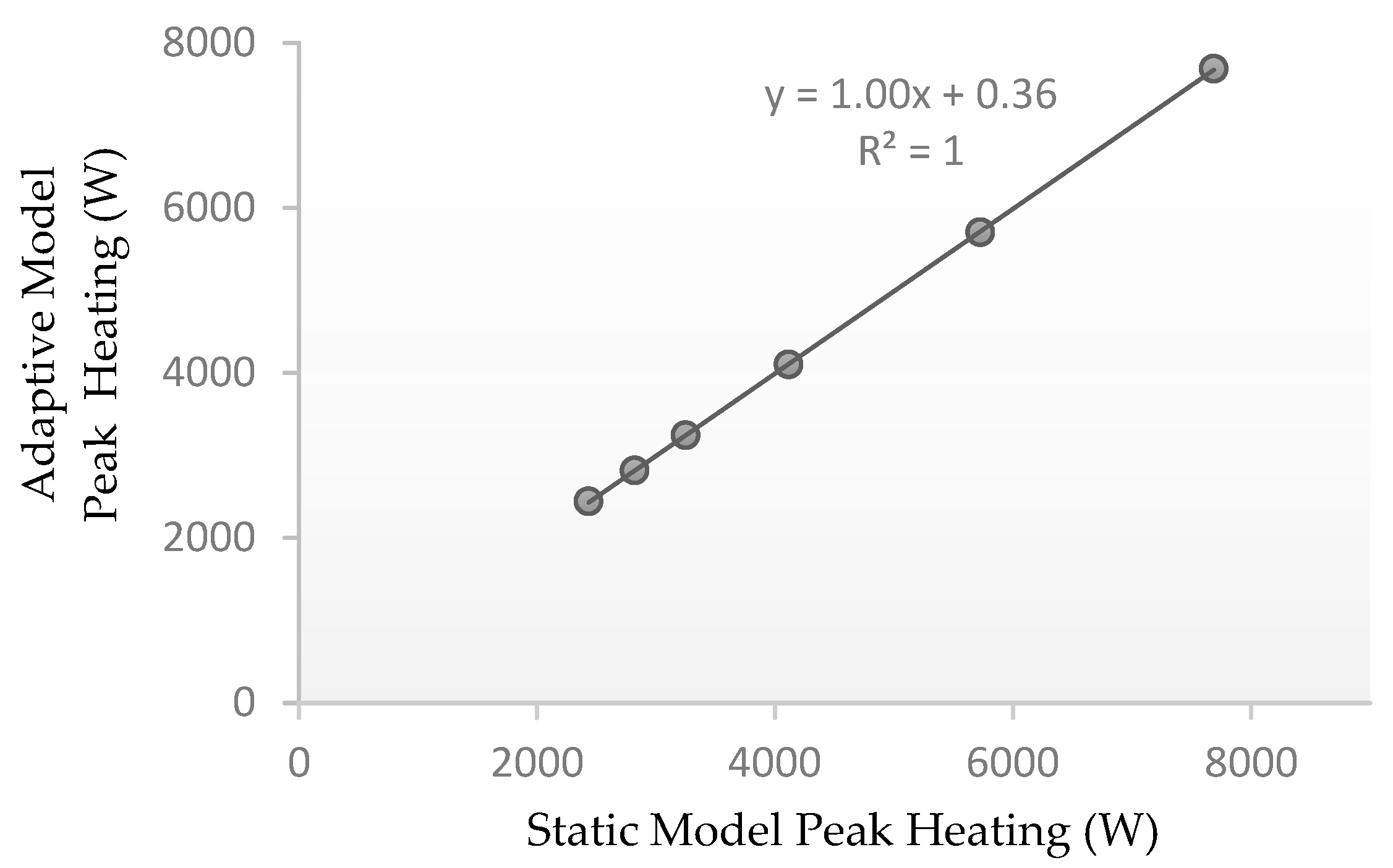
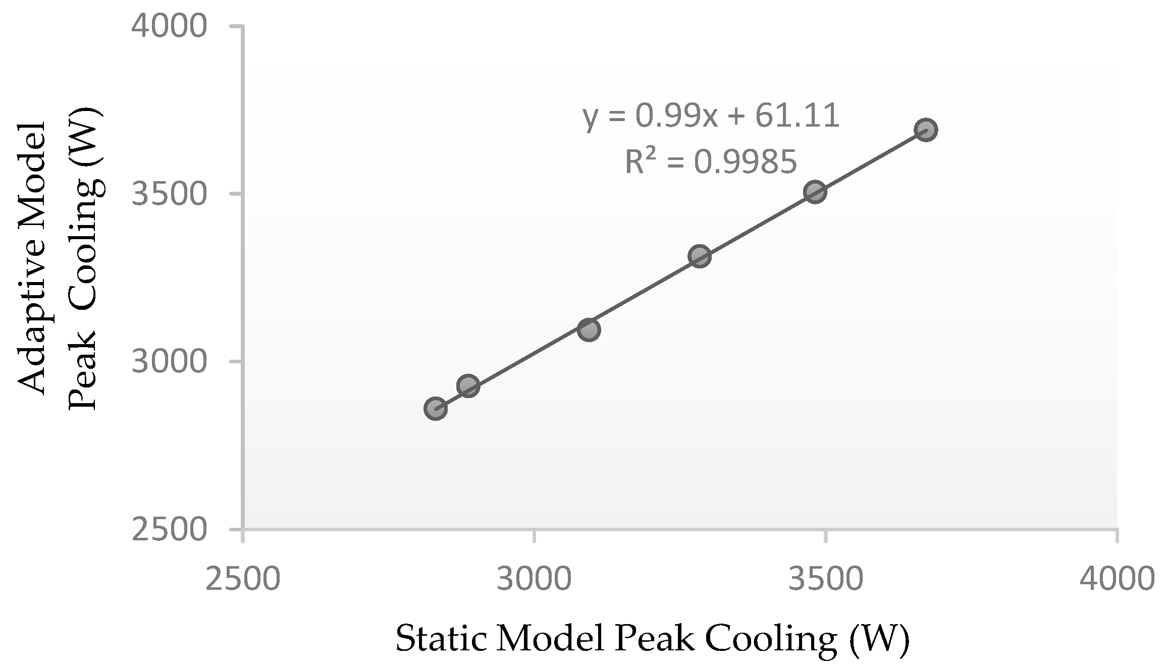
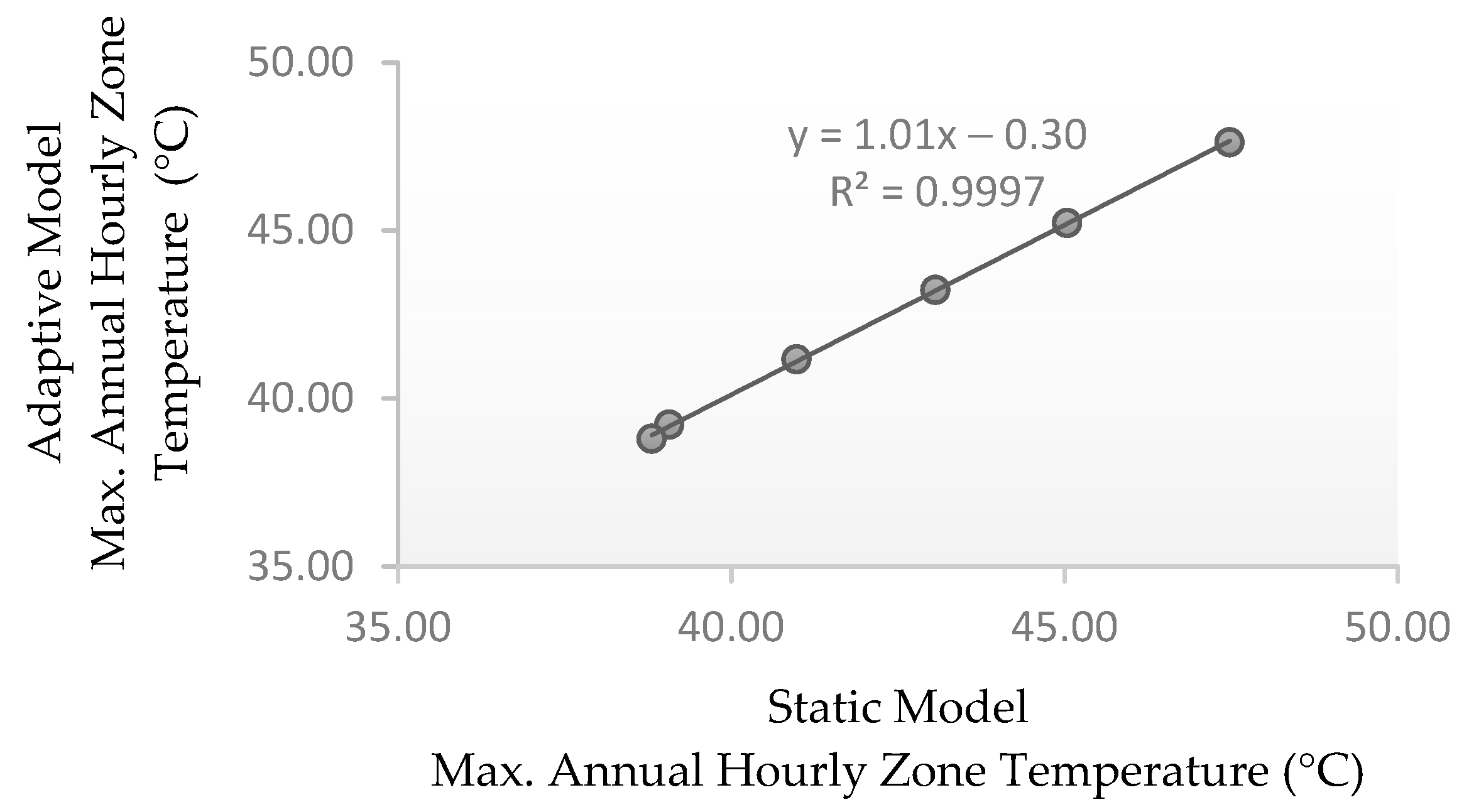
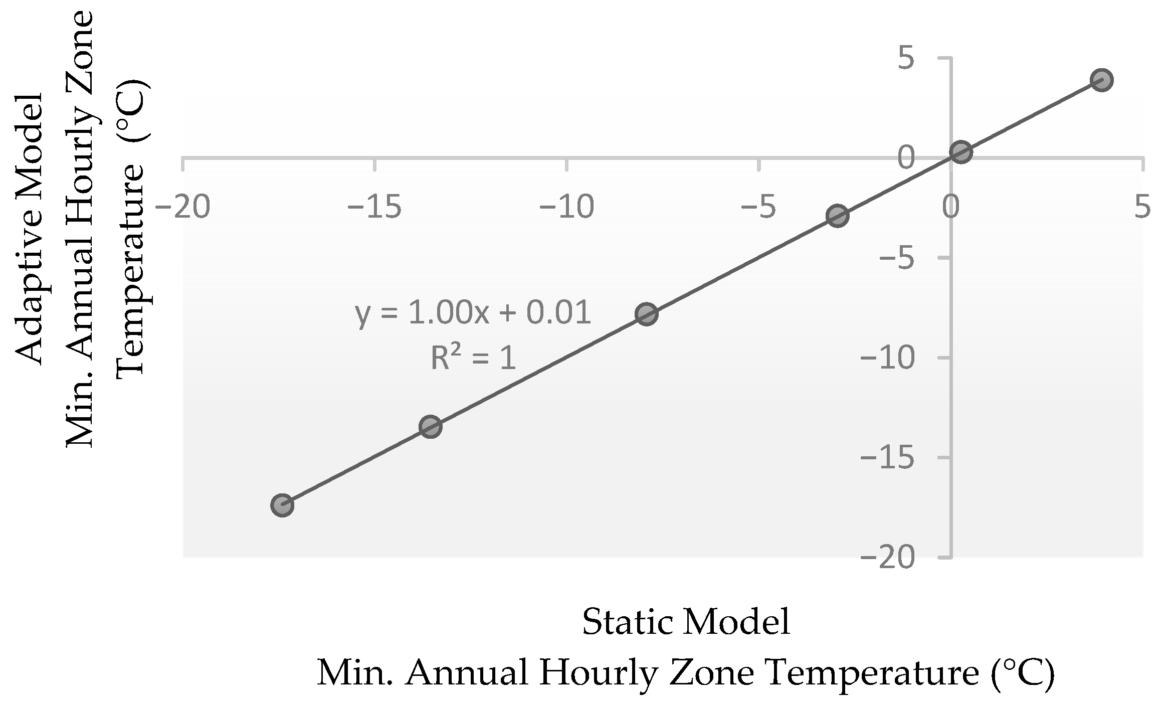
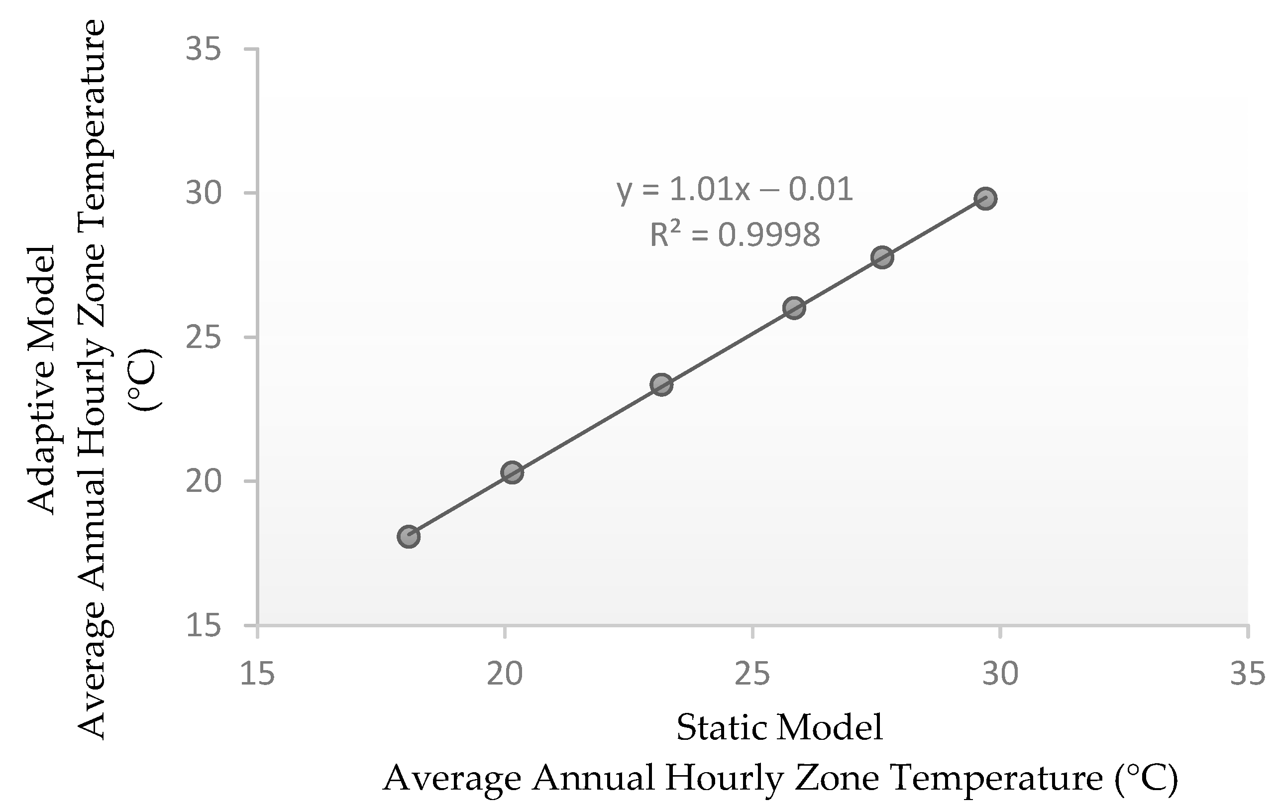
  • Simulate both cases (BesTest900 and 900FF) over a one-year period, for both the Static model and the Adaptive model, to obtain the dependent variables: cooling annual energy demand (kWh), heating annual energy demand (kWh), peak heating (W) and peak cooling (W) for BesTest 900, and maximum annual hourly zone temperature (°C), minimum annual hourly zone temperature (°C), and average annual hourly zone temperature (°C) for BesTest 900FF. It should be noted that when a specific total insulation of the set is chosen for comparison, the Adaptive model must be simulated using the chosen insulation for the entire one-year simulation period, as the insulation cannot be changed during run time in the Static model.
  • Repeat steps 1 through 4 for each insulation thickness in the selected set.
  • Compare the simulation results (dependent variables) by plotting the results for both Static and Adaptive models in the same chart, and adjust a linear regression model for each of the dependent variables. Use the corresponding R-squared (R2) value as a goodness-of-fit measure for the linear regression model to validate the results of the Adaptive model.

3. Results

The results were split into two groups: first and second validation results. For convenience in interpretation, the insulation thickness is presented in millimeters (mm).

3.1. First Validation: BesTest Case 900 and 900FF Original Results for EnergyPlus Version 8.3.0 and Results for EnergyPlus Version 9.5.0

The original EnergyPlus version 8.3.0 results shown in Table 3 and Table 4 were provided by EnergyPlus in [48], and the results for EnergyPlus version 9.5.0 (converted model) were computed by running the EnergyPlus converted model in a Windows 10 environment.
The differences between these two EnergyPlus versions of Case 900, as shown in Table 3, were 1.6% at most (peak cooling). Hence, they were not significant according to software-to-software comparison criteria. The results for version 9.5.0 for all variables moved slightly towards the BesTest average. The results for both versions were closer to the minimum than the average for annual heating and cooling and closer to the average than the minimum or maximum for peak values, considering the sample of software used in BesTest.
The variables for the Case 900FF test for both EnergyPlus versions were the same for maximum and average hourly zone temperatures and almost the same for minimum hourly zone temperature. It can be noted that the −3.9% difference between both versions was not significant since the temperature values were close to zero, increasing the percentage of the difference (Table 4).
The results of BesTest 900FF and BesTest 900 were near the average or close to the midpoint, located between the minimum and the average, except for annual heating, where the EnergyPlus models were close to the minimum value of the software comparison range. Considering that the variables of the BesTest 900 and 900FF original EnergyPlus model were within the range of the software used as a comparison for validation (see note [a] in Table 3 and Table 4), we expected that the newest version 9.5.0 model, converted using a tool developed by EnergyPlus for version conversions, would produce variables for the converted new model that were also within the range. To ensure a rigorous procedure, this assumption was verified, and the Static model was validated as illustrated in this section.

3.2. Second Validation: Case 900 and 900FF Results for Static and Adaptive Models

The % variation between the Adaptive and Static models was calculated as indicated in the following example:
Δ (%) = 100 × Δ (kWh)/Annual Heating Static Model (kWh)
Additionally, the difference was calculated as
Δ (kWh) = Annual Heating Adaptive Model (kWh) − Annual Heating Static Model (kWh)
The results of the Static versus Adaptive model for annual heating, annual cooling, peak heating, and peak cooling are depicted in Table 5. It is clear that when insulation = 1 mm, the Adaptive model behaved exactly as the Static model did. Hence, there was no extra insulation added, and the “SurfaceControl:MovableInsulation” class list had no effect. The differences in percentage between the Static and Adaptive results depended mainly on the amount of extra insulation added in the Adaptive model. For all the variables, starting from 10 mm and ending at 200 mm, the differences (% absolute value) between the Adaptive and Static models decreased as the extra insulation increased, except annual heating, which decreased for 10 mm, peak heating, which rose for 200 mm, and peak cooling, which decreased for 10 mm. When using a high thermal resistance in the “SurfaceControl:MovableInsulation” class list, EnergyPlus uses information from the previous hour’s heat balance (an equation simplification) without a significant effect on the overall final calculations, as stated in [49]. This may result in a slight deviation in peak heating at 200 mm.
The results of the dependent variables, annual heating, annual cooling, peak heating, and peak cooling for the six different insulation thicknesses shown in Table 5 were compared for the Static and Adaptive models by plotting the results and adjusting a linear regression model for each of the variables mentioned above. Figure 4, Figure 5, Figure 6 and Figure 7 show the results for the Static and Adaptive models for each insulation thickness, plotted on the same chart, along with their linear regression lines and linear equations and the corresponding R-squared (R2) values as a goodness-of-fit measure for the linear regression model. For example, each data point in Figure 4 represents the annual heating for the Static model and the corresponding annual heating for the Adaptive model for the same insulation thickness.
The resulting R2 values, presented in Figure 4, Figure 5, Figure 6 and Figure 7, are summarized in Table 6. The R2 values shown in Table 6 are very close to 1.0, indicating that the BesTest 900 variable results for the Adaptive model were statistically equivalent to those of the Static model.
Table 7 presents a comparison between the Static and Adaptive model results for maximum annual hourly zone temperature, minimum annual hourly zone temperature, and average annual hourly zone temperature, as required by the office space model defined by BesTest900FF, with the model modification explained in Section 2.2, for different insulation thicknesses.
The difference in percentage between the Static and Adaptive results depended mainly on the amount of extra insulation added in the Adaptive model except for the maximum annual hourly zone temperature, which maintained the difference (%) almost constant. When insulation = 1 mm, the Adaptive model behaved exactly as the Static model did (i.e., no extra insulation was added).
Starting from 10 mm and ending at 200 mm, the difference (% absolute value) between the Adaptive and Static models for the minimum annual hourly zone temperature increased as the extra insulation increased, except for the result for 200 mm insulation, which decreased. In the case of the average annual hourly zone temperature, the difference decreased as the insulation increased, except for the result for 10 mm insulation.
As stated previously for the BesTest 900 variables, Figure 8, Figure 9 and Figure 10 show the results for the BesTest 900 FF variables of the Static and Adaptive models for each insulation thickness plotted on the same chart, with their linear regression lines and linear equations and the corresponding R-squared (R2) values as a goodness-of-fit measure for the linear regression model.
The resulting R2 values for the linear regression model for each variable, for the Static vs. Adaptive models, are summarized in Table 8. The R2 values shown in Table 8 are all very close to 1.0, indicating that the BesTest 900FF variable results for the Adaptive model are statistically equivalent to those of the Static model.
As can be seen in Table 5 and Table 7, the difference between the Adaptive and the Static models are all less than 4.3%. Considering the goodness-of-fit measure (R2) shown in Table 6 and Table 8, the Adaptive model is statistically equivalent to the Static model for the dependent variables considered in BesTest Case 900 and Case 900 FF, thereby validating the Adaptive model.

4. Adaptive Model Example and Software Framework

The Adaptive model presented and validated in this research, with the same climate, configuration, and parameters as described in Section 2, was used to simulate the total energy demand reduction (heating + cooling) if an adaptive façade with variable thermal resistance for the opaque part of the façade was adopted in the model. First, the optimal insulation thickness for the Adaptive model was obtained and used as the reference for comparison with three other simulation alternatives. The four cases were the following:
Case A: Optimal insulation thickness for minimizing total energy demand (annual heating + annual cooling), considering the same insulation for all four walls (balanced insulation) of the Adaptive model and repeating this on every day of the 365-day simulation period.
Case B: Optimal insulation thickness for minimizing total energy demand (annual heating + annual cooling), considering that the insulation of each of the four walls of the Adaptive model could adopt a different thickness (unbalanced insulation). Each wall repeated the same insulation adopted, on every day of the 365 days of the simulation period.
Case C: Optimal insulation thickness for minimizing total energy demand (annual heating + annual cooling), considering that the insulation was the same for each wall (balanced insulation) and could change every day (adapt) during the 365-day simulation period for minimizing total energy demand.
Case D: The same as Case C but with electrochromic glazing added on both windows of the Adaptive model. The electrochromic glazing considered had two states: fully clear (Clear) and fully tinted (Dark). The parameters were obtained from the SageGlass Classic panel and exported from the International Glazing Database (IGDB), published by the Lawrence Berkeley National Laboratory (LBNL) using the LBNL Window program.
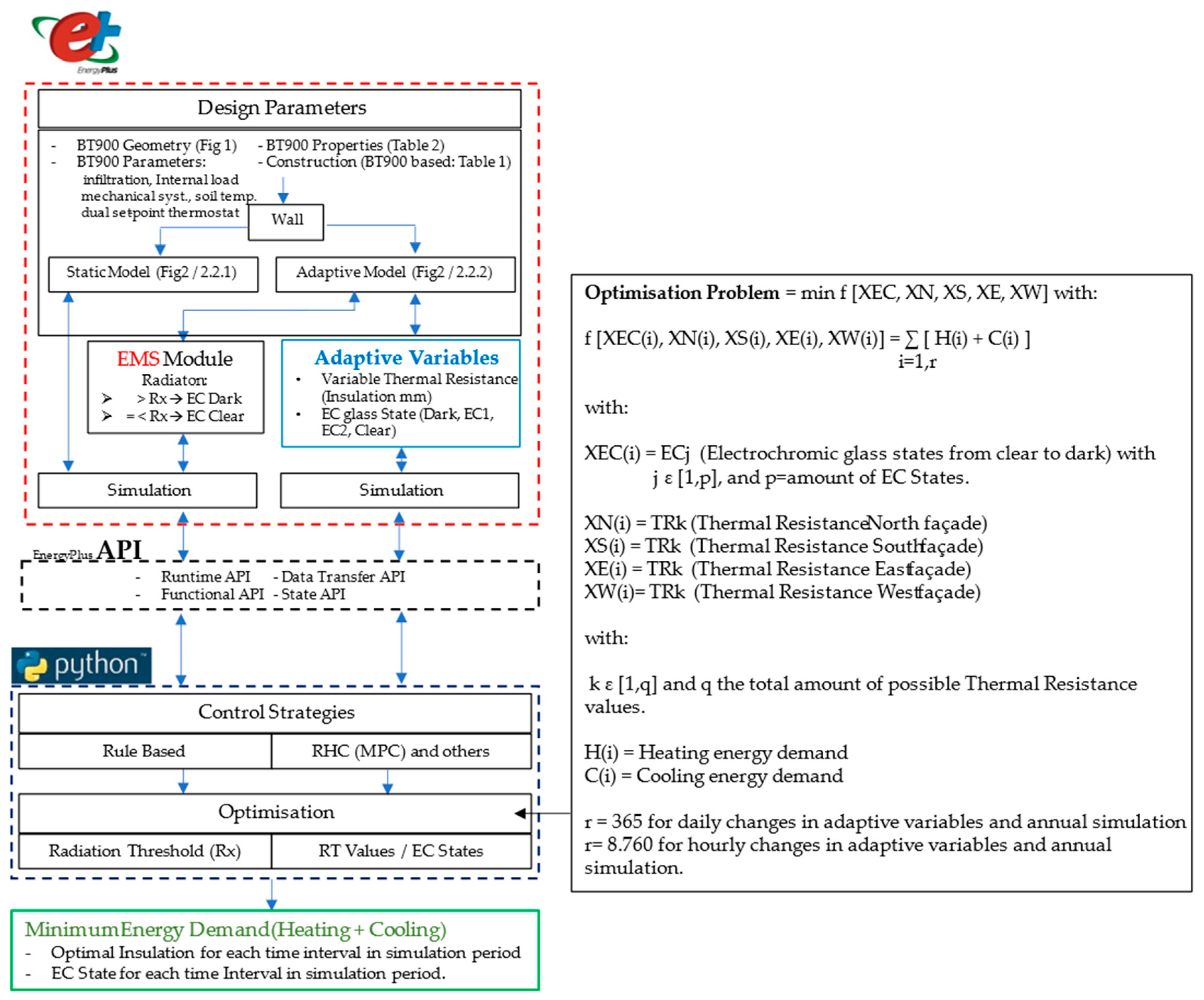
The simulation of the Adaptive model coded in EnergyPlus was executed by a Python version 3.9 program that communicated with EnergyPlus via an EnergyPlus API to call EnergyPlus as a function from Python.
The electrochromic glazing simulation for Case D was carried out using the EnergyPlus Energy Management System (EMS). The EMS program, written in the EnergyPlus Runtime Language (Erl), switched from the Clear state to the Dark state when the Incident Solar Radiation exceeded a radiation threshold (Rx). The optimization to determine the insulation thickness daily values was performed in Python.
The software simulation platform for adaptive façades with variable thermal resistance and electrochromic (EC) glazing is presented in Figure 11.
The results for Cases A, B, C, and D are presented in Table 9.
For Cases C and D, Table 10 shows the different values considered for the insulation thickness and the number of days in the year on which those values were adopted for minimizing energy demand.
The results for Case B show that if unbalanced insulation was considered for this climate, a 3% energy reduction was achieved compared to the balanced insulation of Case A. This was performed by increasing heating energy demand by 93 kWh and reducing cooling energy demand by 220 kWh. Although Cases A and B were not adaptive façade cases, it was interesting to explore the possibilities of unbalanced insulation thickness, such as moving energy demands from cooling to heating.
When an adaptive façade was considered for the Adaptive model (Case C) and the thermal resistance could adapt by changing the insulation thickness once a day, while keeping the same value for the four walls during the day (balanced–adaptive), energy demand was reduced by 26% compared to the optimal insulation thickness of Case A. In Case C, 60% of the time, high (≥150 mm) or low insulation (≤10 mm) was the optimal insulation for reducing total energy demand (heating + cooling).
Finally, Case D (Case C with EC glazing added) led to a 54% energy demand reduction compared to Case A. The heating demand was almost the same as that in Case A, and the cooling energy demand was significantly reduced by switching the EC glazing to the EC Dark state. The presence of the highest insulation thickness (200 mm) was needed for 62% of the year to compensate for less radiation received through windows due to the lower solar transmittance of the EC Clear state compared with Glass Type 1 of the original glass.

5. Discussion

Research on BPS has been conducted in recent years using simplified models such as the ones presented in [39,50,51,52]. This has been performed due to multiple factors such as geometry modeling, result validation, result comparison, the complexity of working with a whole real building, and computation time. The U.S. Department of Energy requested Lawrence Berkeley National Laboratory to prepare a comparative test for the EnergyPlus software with simplified models, according to the ANSI/ASHRAE Standard 140-2011 (BESTEST) [43,44]. The advantage of the BesTest model is the possibility of comparing the results provided by the standard, with the same BesTest model that is being used in a research study, even if a different software is used to model BesTest. The standard considers a software-to-software comparison of the results that are expected to be within a range of acceptable values for software validation [44].
A cellular office room model with and without the EnergyPlus “SurfaceControl:MovableInsulation” class list was analyzed in [39], and as the author stated, “the main purpose of the analysis was to compare the temperatures at the interface between the insulation layer and the concrete, and along the concrete layer.” On the other hand, in this research, the Adaptive model is based on the standardized BesTest Case 900 and 900FF models, with the EnergyPlus “SurfaceControl:MovableInsulation” class list added. This research not only complements the results described in [39] but also presents a quantitative validation for the “SurfaceControl:MovableInsulation” class list. However, adding the dependent variables related to energy demand, peak demand, and temperatures inside the model zone, and checking that the Adaptive model results compared with the expected results provided by BesTests, as part of the validation process, led to an EnergyPlus error that is described in the following paragraph. This error could not be found in [39] due to qualitative validation being used instead of quantitative validation. A transitory solution for using the “SurfaceControl:MovableInsulation” class list for a variable-thermal-resistance model, where no extra insulation was added, was also found and successfully used to obtain the result of the Adaptive model for a total insulation thickness of 1 mm.
In the Adaptive model validated in this research, to have a final insulation of 1 mm, the Schedule1 parameter should equal 0.0 so that an extra amount of insulation is not added (see Section 2.2), and the final insulation is the 1 mm base insulation that is always present (see 
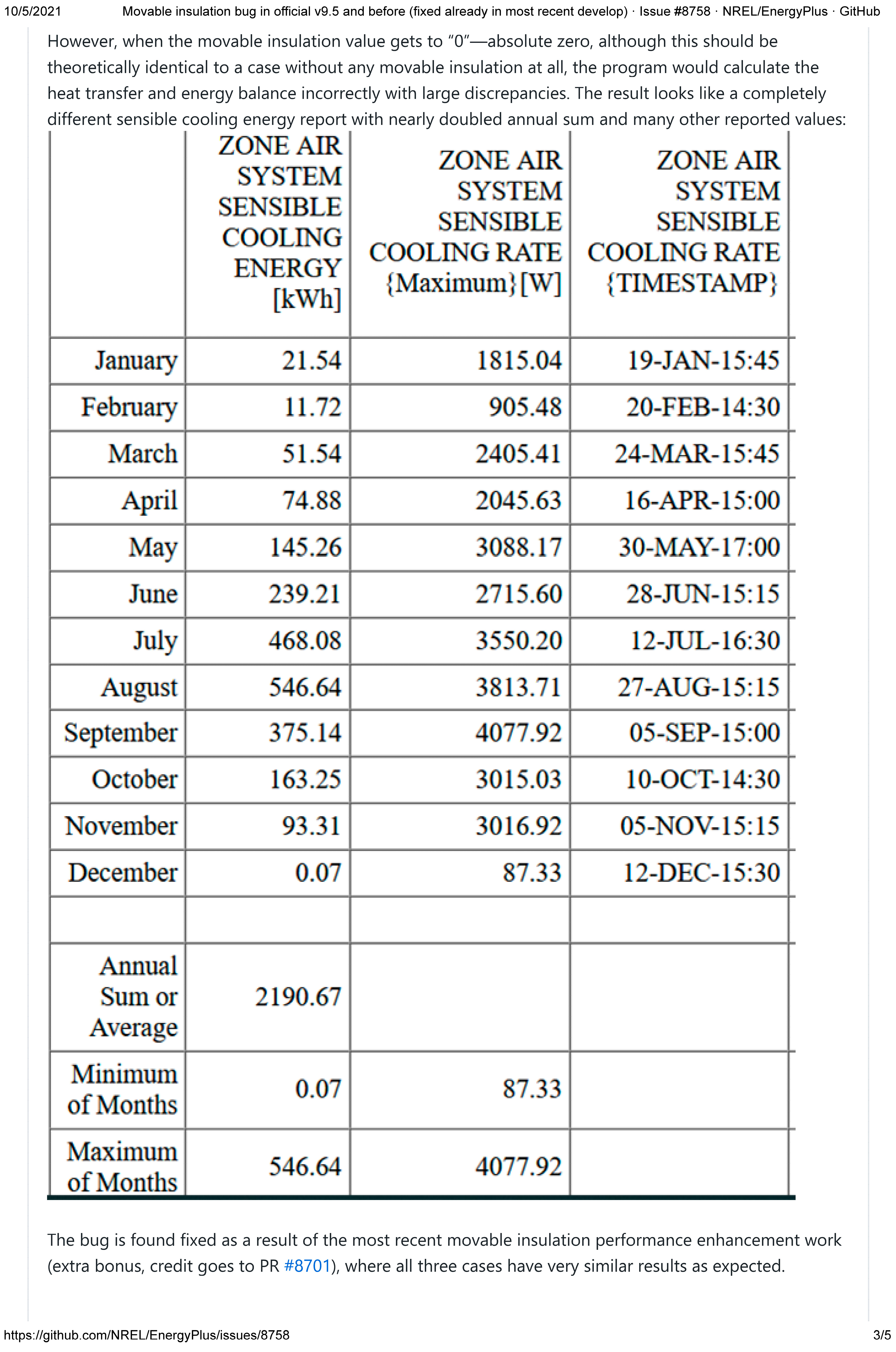
Figure 2). It is important to note that when Schedule1 = 0.0 was set in the EnergyPlus Adaptive model, the results were very different from those of the Static model and also outside the logical range of expected results, as seen in note (a) of 
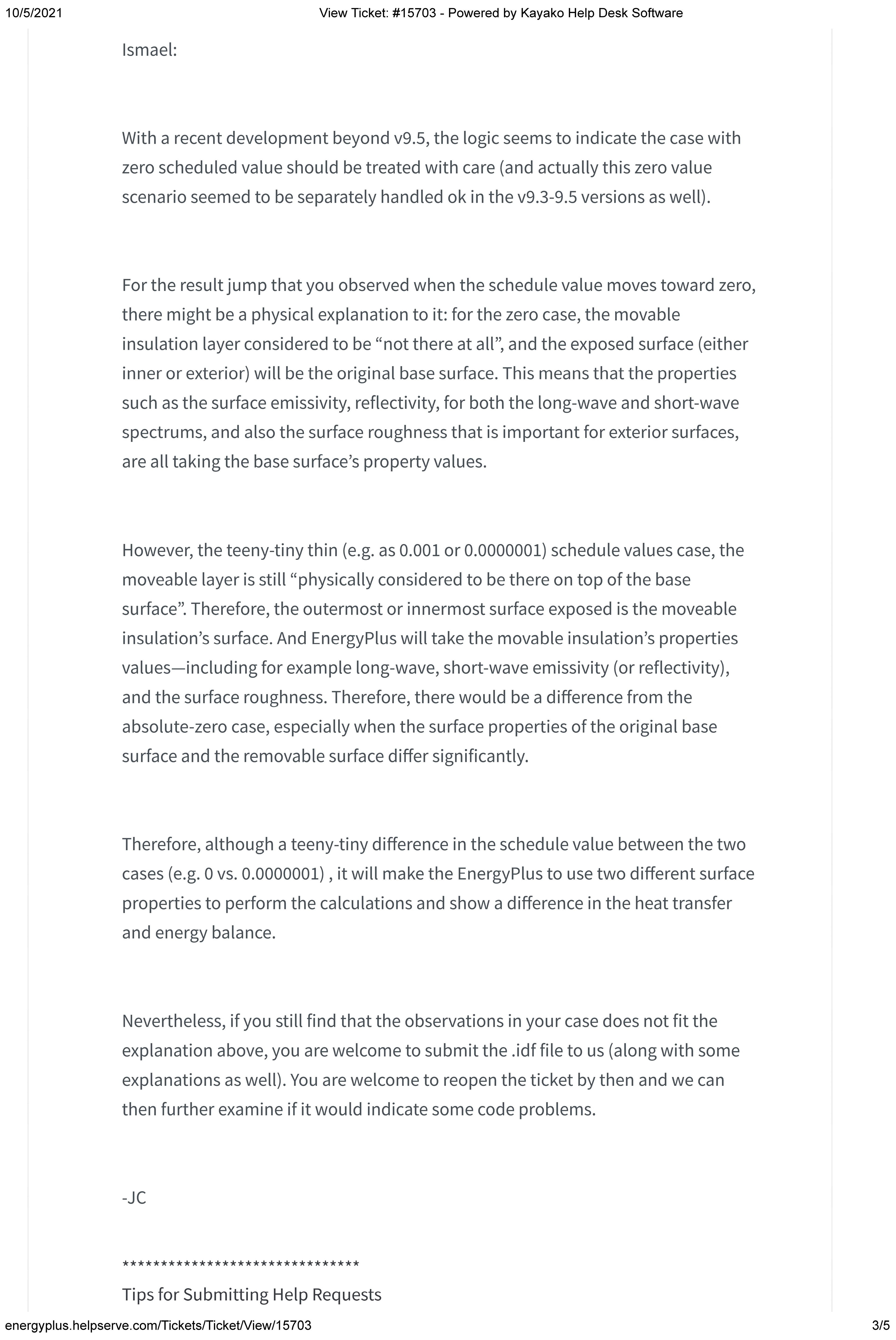
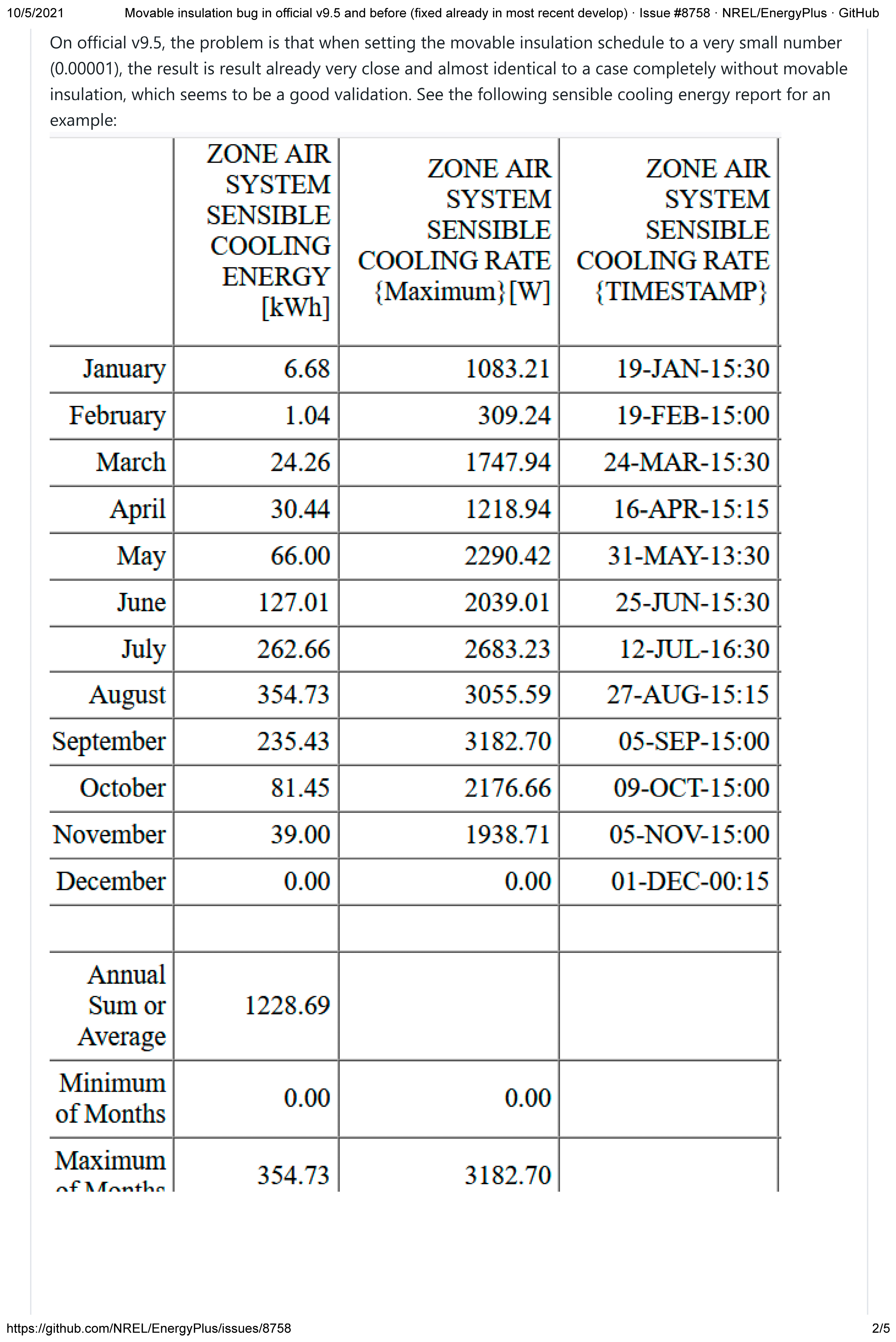
Table 5. In contrast, the other results (total insulation = 10 mm, 30 mm, 61.5 mm, 100 mm, 200 mm) were very close to the Static model results. EnergyPlus documentation for version 9.5.0 indicates that the multiplier could be any positive real number starting from 0.0. If a value for Schedule1 = 0.0000001 was set, the model results for 1 mm insulation thickness were the same for both the Static and Adaptive models, as shown in Table 5 and Table 7. Moreover, a Schedule1 floating value greater than 0.0, such as 0.001, produced results very near the Static model results. Considering the results of 
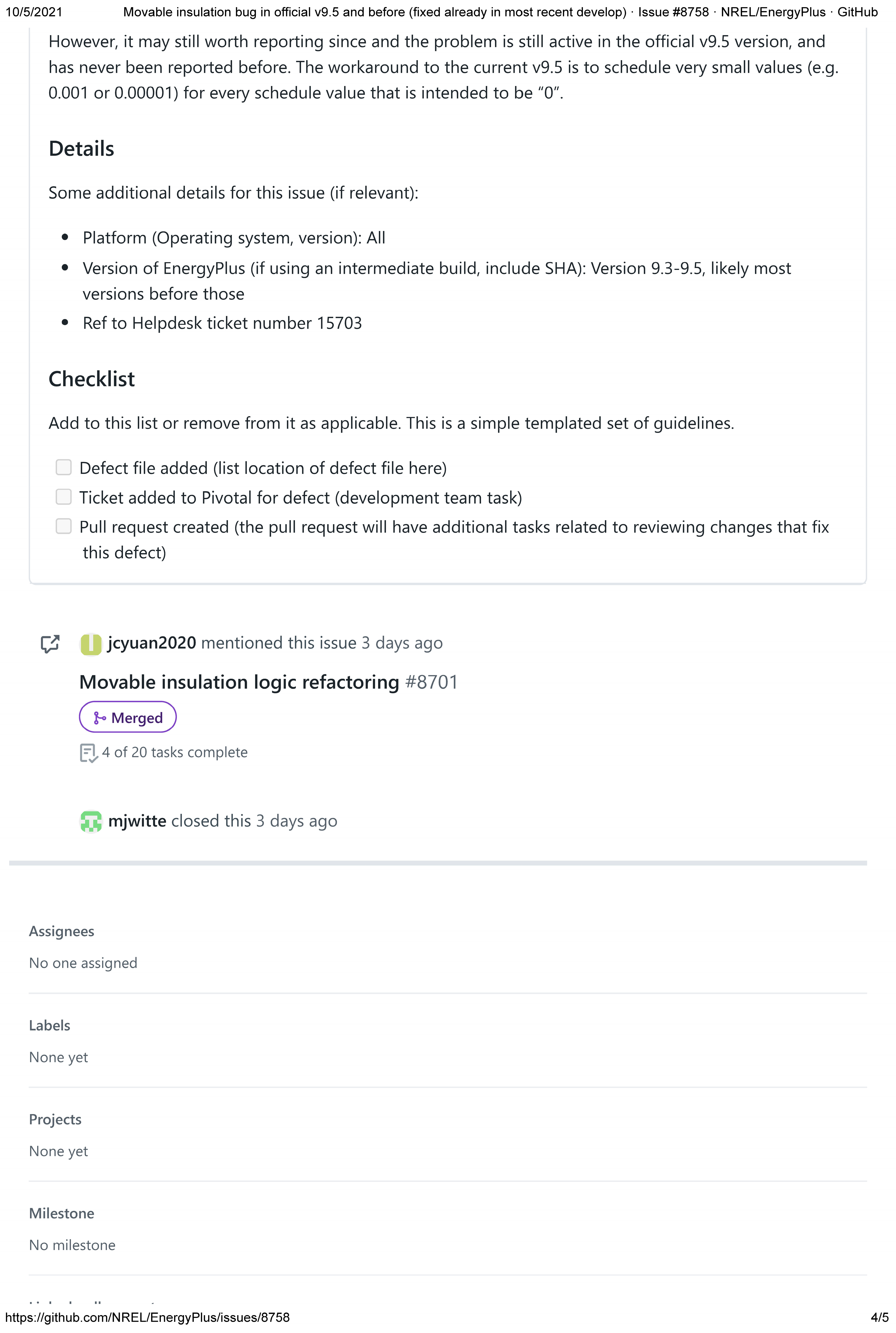
Table 5 note (a), setting Schedule1 = 0.0 in the SurfaceControl:MovableInsulation class list produced an EnergyPlus malfunction, and a partial solution consisted of considering a floating value greater than 0.0 but very close to it. The error was fully documented and sent to EnergyPlus support. On May 7th, 2021, it was confirmed to be a “code bug for the official EnergyPlus v9.5 and before” (see Appendix B for the report to EnergyPlus support and Appendix C for the official answer and confirmation from EnergyPlus regarding the software malfunction reported). The error was fixed, and the new code was included in the following EnergyPlus versions. It was also confirmed from EnergyPlus that using a Schedule1 positive floating value very close to 0.0 would give results “very close and almost identical to a case completely without movable insulation, which seems to be a good validation”. After finding a solution for the case Schedule1 = 0.0, where no extra insulation was added for setting up the Adaptive model for a total insulation = 1 mm, Table 5 and Table 7’s results for this case were generated using Schedule1 = 0.0000001 and were confirmed by EnergyPlus to be good validation. It is relevant that all previous research that used the SurfaceControl:MovableInsulation class list produced an EnergyPlus malfunction when Schedule1=0.0 was set (no extra insulation added), so those results were not correct for those simulations.
The framework presented in this study is entirely based on open-source free software: EnergyPlus, Python, and an EnergyPlus API for communication between them, with all the capabilities described in other frameworks like the one described in [39], which is based on the commercial software MATLAB 2013b and the free software EnergyPlus. One of the advantages of using Python is the availability of a collection of modules and fully documented applications, such as optimization algorithms and functions. There is a large software and research community around Python that develops and tests a wide range of applications that could be used to implement levels 1, 2, and 3 described in [39]. Moreover, the EnergyPlus API used in this research allows Python code to call and use EnergyPlus as a function, with almost unlimited possibilities for new technologies and model simulations, the implementation of new algorithms, and full statistical analysis and database management using existing modules and applications already developed in Python with free access and support. Finally, communicating EnergyPlus with Python is easier with the EnergyPlus API than with the software for MATLAB for communicating and co-simulating with EnergyPlus. The capability of Python with an API to call EnergyPlus as a function provides a powerful platform for building performance simulations of adaptive façades.
From the examples described in Section 4, although from an energy point of view, unbalanced insulation (Case B) is more effective than balanced insulation (Case A), the adoption of an unbalanced insulation design alternative depends on local regulations and the convenience after a comparative cost analysis is made (energy savings versus the amount of insulation costs), among other technical issues, such as thermal bridging risks. In countries like Chile, regulations and standards are based on the amount of insulation that walls must provide according to the climate zone where a projected building will be constructed. An unbalanced insulation design option could lead to an insulated wall that falls below the local regulations, and the rest of the walls exceed the standard.
The example described in Section 4, in Case D, illustrates the potential of an adaptive façade in its opaque and glazed parts to reduce energy demand towards 15 kWh/m2-year or less, expected for an nZEB building. The energy reduction could be higher if more states for the EC were considered. Additional improvement could be achieved if an algorithm such as Receding Horizon Control (RHC) was used to command the EC switching decision from one state to another, providing a solution to an optimization problem. In the example of Section 4, the EC switched when the Incident Solar Radiation exceeded a certain threshold (“rule-based” control strategy), and this was not the result of a simultaneous optimization problem solution, considering the insulation thickness and the EC state.

6. Conclusions

A simplified office model for simulating a variable-thermal-resistance façade was proposed based on the validated model of BesTest Cases 900 and 900FF. A minor modification of BesTest Case 900 was made by adding the EnergyPlus SurfaceControl:MovableInsulation class list and removing the Wood Siding present in the Case 900 model, obtaining a model similar to an EIFS with variable thermal resistance. The model and the EnergyPlus “SurfaceControl:MovableInsulation”class list used were quantitatively validated, and the process was fully documented, including EnergyPlus code modification. Moreover, the validation process allowed the discovery of an EnergyPlus software bug for the mentioned class list. The error condition and an example were reported to EnergyPlus, including a partial solution for using the class list. The bug was confirmed and the partial solution validated by EnergyPlus, after which the final solution was implemented in the following versions of EnergyPlus.
The results for the converted BesTest Case 900 and BesTest 900FF, shown in Table 3 and Table 4, were within the range of software comparison results presented in [48], so the converted model (coded in EnergyPlus version 9.5.0) was validated according to those criteria. This was expected because the only difference between the validated model and the converted model is the new version of EnergyPlus (version 9.5.0) used in the converted model code, also considering that the conversion was performed using an EnergyPlus version conversion program.
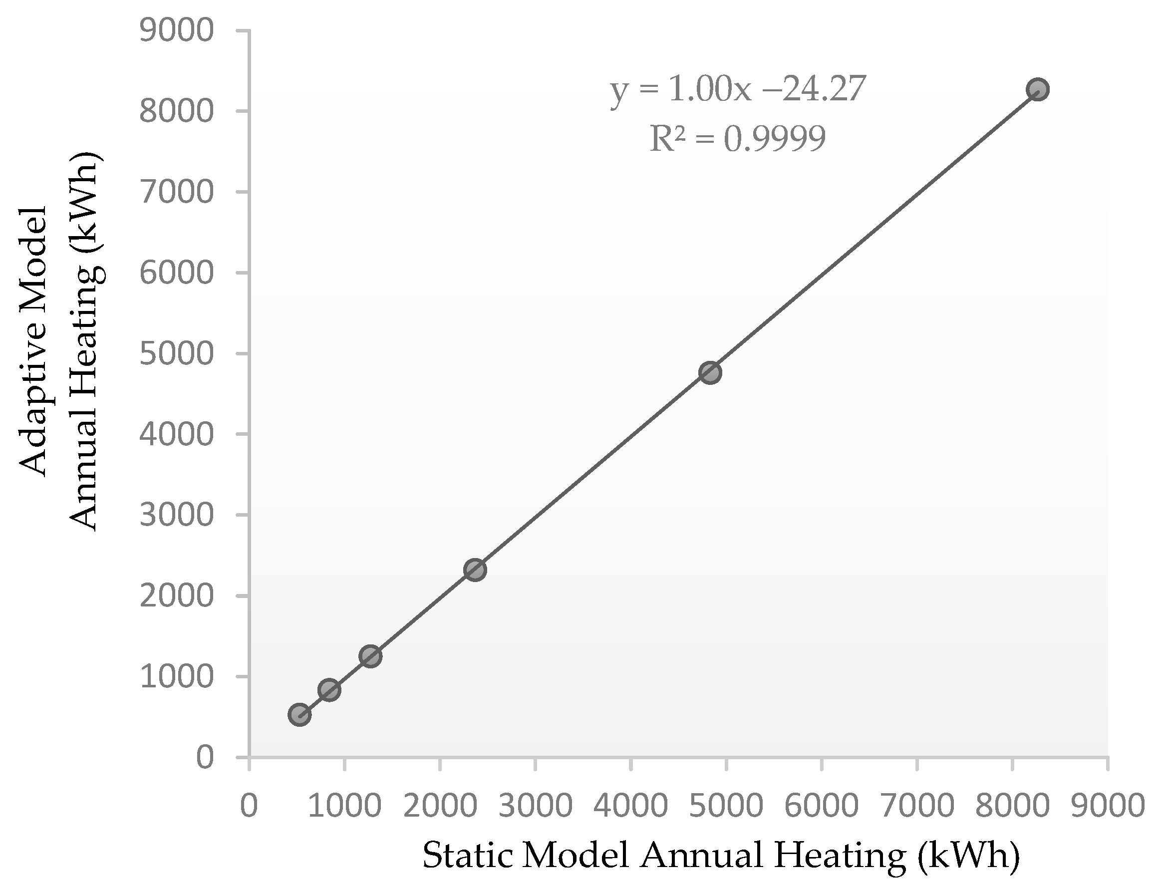
The results for the Static model and the Adaptive model, shown in Table 5 and Table 7, were statistically compared using “goodness-of-fit linear regression”. The R2 values presented in Table 6 and Table 8 show that the Adaptive model behavior was equivalent to the Static model behavior, so the proposed Adaptive variable thermal resistance model, which uses the EnergyPlus “SurfaceControl:MovableInsulation”, was successfully validated according to the software comparison criteria and considering the output variables used in BesTest Case 900 and Case 900FF (annual heating, annual cooling, peak heating, peak cooling, maximum annual hourly zone temperature, minimum annual hourly zone temperature, and average annual hourly zone temperature).
The example presented in Section 4 was simulated in one climate only. Considering that the energy reduction potential of an adaptive façade is climate-dependent, changes in the adaptive façade performance are expected when changing the location to another climate. Further research could evaluate the results of the Adaptive model described in this research for different climates and with different layers for the building construction envelope, comparing them with a Static model and also addressing the thermal bridging effect in a variable-thermal-resistance model. A second limitation of this study is the use of a simplified geometry instead of a complete building example. Since the variable-thermal-resistance technology is still under development, it is also desirable to have a study of the potential of this technology for different full-scale building topologies (i.e., buildings with different Window-to-Wall Ratios and orientations) and compare cooling and heating energy demand parameters such as kWh/m2-year of each topology with a simplified model based on a BesTest Case, to have a clear view of the possible limitations of using a simplified model for each full-scale building topology. To help better integrate the model into real-world applications, a future experimental validation should be conducted using a real-scale model that incorporates energy consumption data collection for results comparison.
Another limitation of the research is the number of modules considered for unbalanced insulation. Only four modules were considered, and each of them covered the entire North, South, East and West walls. The validated model presented in this study could also be used to investigate the effect of configuring each wall with several small panels to reduce energy demand, thereby improving convection for natural ventilation.
The Adaptive model validated in this research could be used to explore the energy reduction potential of an adaptive façade in its opaque and glazed parts. As shown in the example in Section 4, the energy demand was reduced from 79 kWh/m2-year to 36 kWh/m2-year if both technologies were used simultaneously. The reduction could be higher and move towards the expected 15 kWh/m2-year or less for an nZEB, if an RHC algorithm is used. In this scenario, the adaptive frequency of a daily change is reduced to 1 h, more states for the EC glazing are considered, and the state switching decision for the EC glazing responds to an optimization problem solved in conjunction with the insulation thickness decision.
The results from the model simulation for various climates and different thermal resistances, presented like those in Table 10, serve as a reference for developers of variable-thermal-resistance technologies applicable to building façades. Developers could focus on achieving the thermal resistance values that significantly reduce energy demand. Moreover, these findings provide a foundation for the development of tailored variable-thermal-resistance products specifically designed to address particular climate groups.
Emerging technologies or those under development like variable-thermal-resistance adaptive façades could be accelerated if research results yield interesting energy demand reductions that could help achieve building performance goals.

7. Future Directions for Adaptive Façades with Variable Thermal Resistance Development

  • A wide range of thermal resistances including very low and very high thermal resistance.
  • Thermal resistance changes triggered by a control signal.
  • Fast response time (a few minutes at most).
  • Low operational energy.
  • Low noise and vibrations during transition.
  • Low maintenance requirements.
  • Tax incentives for developers of adaptive façade technology, encouraging the early adoption of emerging material technologies in the design of adaptive façades.
  • Thermal requirements for the construction of new buildings considering optimal unbalanced insulation for different weather conditions and façade orientations for static façades. They could also consider a simplified model and a standardized procedure for adaptive façade energy savings calculations to verify whether the regulatory requirements are met.

Author Contributions

Conceptualization, I.P.M., A.P.-F. and L.M.-R.; methodology, I.P.M. and A.P.-F.; Software, I.P.M.; Validation, I.P.M.; Formal Analysis, I.P.M.; Investigation, I.P.M.; Writing—Original Draft, I.P.M.; Writing—Review, A.P.-F. and L.M.-R.; Writing—Review and Editing, L.M.-R.; Visualization, I.P.M.; Supervision, A.P.-F. All authors have read and agreed to the published version of the manuscript.

Funding

This work was supported by Vicerrectoría de Investigación y Doctorados de la Universidad San Sebastián–Fondo USS-FIN-25-APCS-22.

Data Availability Statement

For data supporting the reported results, please contact ipmackay@gmail.com.

Conflicts of Interest

The authors declare no conflict of interest.

Abbreviations

The following abbreviations are used in this manuscript in order of appearance:
EIFSExternal Insulation Finishing System
CABSClimate-Adaptive Building Shell
nZEBNearly-zero-energy Buildings
NZEBNet-zero-energy Buildings
ECElectro-chromic
BPSBuilding Performance Simulation
IGDBInternational Glazing Database
LBNLLawrence Berkeley National Laboratory
APIApplication Programming Interface
EMSEnergy Management System
RxIncident Solar Radiation Threshold
RHCReceding Horizon Control
MPCModel Predictive Control

Appendix A

This appendix illustrates the EnergyPlus code differences between the BesTest 900 original code and the Static model. The EnergyPlus code for an Adaptive model equivalent to the Static model is also presented. Table A1 shows the EnergyPlus code differences between the BesTest 900 model and the Static model (Wood Siding-1 removed).
Table A2 shows the EnergyPlus code difference between the Adaptive and the Static models in the construction and material definitions. It should be noted that in the Static model example, the insulation is 61.5 mm, whereas in the Adaptive model, the insulation is 1 mm. Therefore, the SurfaceControl:MovableInsulation class list was added, as shown in Table A3, to add extra insulation and achieve the desired total insulation that the Schedule1 multiplier could vary.
Table A1. Construction EnergyPlus definitions for the BesTest 900 original model and the Static model.
BesTest 900 ModelStatic Model
FieldObj1FieldObj1
NameHWWALLNameHWWALL
Outside LayerWOOD SIDING-1Outside LayerFOAM INSULATION
Layer 2FOAM INSULATIONLayer 2CONCRETE BLOCK
Layer 3CONCRETE BLOCKLayer 3-
Layer 4-Layer 4-
Layer 8 Layer 8
Layer 9 Layer 9
Layer 10 Layer 10
Table A2. EnergyPlus definitions for construction and materials in the (a) Adaptive and (b) Static models.
(a)(b)
FieldUnitsObj1Obj2FieldUnitsObj1Obj2
Name CONCRETE BLOCKFOAM INSULATIONName CONCRETE BLOCKFOAM INSULATION
Roughness RoughRoughRoughness RoughRough
Thicknessm0.10.001Thicknessm0.10.0615
ConductivityW/m-k0.510.04ConductivityW/m-k0.510.04
DensityKg/m3140010DensityKg/m3140010
Specific HeatJ/kg-K10001400Specific HeatJ/kg-K10001400
Thermal Absorptance 0.90.9Thermal Absorptance 0.90.9
Solar Absorptance 0.60.6Solar Absorptance 0.60.6
Visible Absorptance 0.60.6Visible Absorptance 0.60.6
Table A3. Adaptive model example: EnergyPlus SurfaceControl:MovableInsulation class list added.
[0004]SurfaceControl:MovableInsulationExplanation of Object and Current Field
[0001]OtherEquipmentObject Description: Exterior or Interior Insulation on opaque surfaces
Field ID: A4
Select from the list of objects
This field is required.
[0001]ZoneInfiltration:DesignFlowRate
[0001]ZoneControl:Thermostat
[0001]ThermostatSetPoint:DualSetPoint
[0001]ZoneHVac:IdealLoadsAirSystem
[0001]ZoneHVac:EquipmentList
[0001]ZoneHVac:EquipmentConnections
[0001]NodeList
FieldObj1Obj2Obj3Obj4
Insulation TypeOutsideOutsideOutsideOutside
Surface NameZONE SURFACE NORTHZONE SURFACE SOUTHZONE SURFACE EASTZONE SURFACE WEST
Material NameFOAM INSULATIONFOAM INSULATIONFOAM INSULATIONFOAM INSULATION
Schedule NameSchedule1Schedule1Schedule1Schedule1
Considering that the insulation in the Adaptive model is 1 mm (Table A2), to achieve a total insulation of 61.5 mm in the Adaptive model, the Schedule1 multiplier definition in EnergyPlus code must be 60.5, as shown in Table A4. The extra insulation added by the SurfaceControl:MovableInsulation class list is calculated by multiplying the insulation (1 mm) by Schedule1 (60.5), so the total insulation is
Total Insulation = Insulation + Extra Insulation
Total Insulation = Insulation + Insulation × Schedule1 =
1 mm + 1 mm × 60.5 = 61.5 mm
Varying the Schedule1 multiplier the Adaptive model could vary its total insulation. Consequently, the total thermal resistance of the insulation layer is also variable, and its value depends on the definition of the Schedule1 value.
Table A4. Adaptive model example: EnergyPlus code for Schedule1 multiplier definition.
FieldUnitsObj1
Name Schedule1
Schedule Type Limits Name
Hourly Valuevaries60.5

Appendix B

This appendix details the first author’s communications with EnergyPlus support regarding the detection of an EnergyPlus code bug during the model’s validation.
Figure A1. Communications with EnergyPlus support for the code bug reported.
Energies 18 02682 g0a1aEnergies 18 02682 g0a1bEnergies 18 02682 g0a1cEnergies 18 02682 g0a1dEnergies 18 02682 g0a1e

Appendix C

This appendix includes the EnergyPlus code bug report.
Figure A2. EnergyPlus official report and transitory solution provided by principal author.
Energies 18 02682 g0a2aEnergies 18 02682 g0a2bEnergies 18 02682 g0a2cEnergies 18 02682 g0a2dEnergies 18 02682 g0a2e

References

  1. European Parliament and the Council of the EU. Directive (EU) 2024/1275 of the European Parliament and of the Council of 24 April 2024 on the Energy Performance of Buildings. 2024. Available online: http://data.europa.eu/eli/dir/2024/1275/oj (accessed on 19 November 2024).
  2. Ibrahim, M.M.; Suarez-Lopez, M.J.; Hanafy, A.A.; William, M.A. Optimizing NZEB performance: A review of design strategies and case studies. Results Eng. 2025, 25, 103950. [Google Scholar] [CrossRef]
  3. Moghaddam, S.A.; Serra, C.; Gameiro da Silva, M.; Simões, N. Comprehensive Review and Analysis of Glazing Systems towards Nearly Zero-Energy Buildings: Energy Performance, Thermal Comfort, Cost-Effectiveness, and Environmental Impact Perspectives. Energies 2023, 16, 6283. [Google Scholar] [CrossRef]
  4. Andrade, B.P.B.; Piran, F.A.S.; Lacerda, D.P.; Sellitto, M.A.; Campos, L.M.d.S.; Siluk, J.C.M. Analysis of methods to transform existing buildings into Nearly Zero Energy Buildings (NZEB). Energy Effic. 2025, 18, 3. [Google Scholar] [CrossRef]
  5. Lyu, Y.J.; Xu, W.; Zhang, S.C.; Sun, D.Y.; Hou, Y.B. Review on the recent progress of nearly zero energy building frontiers in China. Sci. China Technol. Sci. 2024, 67, 2620–2636. [Google Scholar] [CrossRef]
  6. Brown, D.; Tokede, O.; Li, H.X.; Edwards, D. A systematic review of barriers to implementing net zero energy buildings in Australia. J. Clean. Prod. 2024, 467, 142910. [Google Scholar] [CrossRef]
  7. Gobierno de Chile; Ministerio de Energía. Plan Nacional De Eficiencia Energética 2022–2026, Santiago, Chile. February 2022. Available online: https://energia.gob.cl/ley-ee (accessed on 25 March 2025).
  8. Perino, M.; Serra, V. Switching from static to adaptable and dynamic building envelopes: A paradigm shift for the energy efficiency in buildings. J. Facade Des. Eng. 2015, 3, 143–163. [Google Scholar] [CrossRef]
  9. Tahmasbi, F.; Khdair, A.I.; Aburumman, G.A.; Tahmasebi, M.; Thi, N.H.; Afrand, M. Energy-efficient building façades: A comprehensive review of innovative technologies and sustainable strategies. J. Build. Eng. 2025, 99, 111643. [Google Scholar] [CrossRef]
  10. Zhang, Y.; Ma, G.; Wu, G.; Liu, S.; Gao, L. Thermally adaptive walls for buildings applications: A state of the art review. Energy Build. 2022, 271, 112314. [Google Scholar] [CrossRef]
  11. Park, B.; Srubar, W.V.; Krarti, M. Energy performance analysis of variable thermal resistance envelopes in residential buildings. Energy Build. 2015, 103, 317–325. [Google Scholar] [CrossRef]
  12. Gao, M.; Zhao, L.; Gao, G.; Jin, R.; Nie, Z. A method for achieving optimal thermal performance of adaptive opaque facades based on monthly loads across China. J. Build. Eng. 2025, 102, 111813. [Google Scholar] [CrossRef]
  13. Gonçalves, M.; Figueiredo, A.; Almeida, R.M.S.F.; Vicente, R. Dynamic façades in buildings: A systematic review across thermal comfort, energy efficiency and daylight performance. Sustain. Energy Rev. 2024, 199, 114474. [Google Scholar] [CrossRef]
  14. Voigt, M.P.; Chwalek, K.; Roth, D.; Kreimeyer, M.; Blandini, L. The integrated design process of adaptive façades—A comprehensive perspective. J. Build. Eng. 2023, 67, 106043. [Google Scholar] [CrossRef]
  15. Faragalla, A.M.A.; Asadi, S. Biomimetic Design for Adaptive Building Façades: A Paradigm Shift towards Environmentally Conscious Architecture. Energies 2022, 15, 5390. [Google Scholar] [CrossRef]
  16. Wang, P.; Liu, Z.; Zhang, L.; Zhao, C.; Jiang, X.; Li, B. Adaptive building envelope combining variable transparency shape-stabilized PCM and reflective film: Parameter and energy performance optimization in different climate conditions. Energy Convers. Manag. 2024, 299, 117907. [Google Scholar] [CrossRef]
  17. Shahin, H.S.M. Adaptive building envelopes of multistory buildings as an example of high performance building skins. Alex. Eng. J. 2019, 58, 345–352. [Google Scholar] [CrossRef]
  18. Voigt, M.P.; Roth, D.; Kreimeyer, M. Decision Support for Defining Adaptive Façade Design Goals in the Early Design Phase. Energies 2023, 16, 3411. [Google Scholar] [CrossRef]
  19. Kadhim, B.M.; Al Maamory, A.S.; Al Ghaban, A.M. Advancing adaptive facades for a sustainable future in building design. Edelweiss Appl. Sci. Technol. 2025, 9, 801–845. [Google Scholar] [CrossRef]
  20. Dehwah, A.H.A.; Krarti, M. Energy performance of integrated adaptive envelope technologies for commercial buildings. J. Build. Eng. 2023, 63, 105535. [Google Scholar] [CrossRef]
  21. Loonen, R.C.G.M.; Trčka, M.; Cóstola, D.; Hensen, J.L.M. Climate adaptive building shells: State-of-the-art and future challenges. Renew. Sustain. Energy Rev. 2013, 25, 483–493. [Google Scholar] [CrossRef]
  22. Feng, K.; Yanfei, M.; Zhang, L.; Liu, Y. Electrically Controlled Smart Window for Seasonally Adaptive Thermal Management in Buildings. Small 2024, 21, e2407033. [Google Scholar] [CrossRef]
  23. Shum, C.; Zhong, L. A review of smart solar shading systems and their applications: Opportunities in cold climate zones. J. Build. Eng. 2023, 64, 105583. [Google Scholar] [CrossRef]
  24. Magri, E.; Buhagiar, V.; Overend, M. The Potential of Switchable Glazing in Cooling Dominated Climates. J. Phys. Conf. Ser. 2023, 2600, 132005. [Google Scholar] [CrossRef]
  25. Tällberg, R.; Jelle, B.P.; Loonen, R.; Gao, T.; Hamdy, M. Comparison of the energy saving potential of adaptive and controllable smart windows: A state-of-the-art review and simulation studies of thermochromic, photochromic and electrochromic technologies. Sol. Energy Mater. Sol. Cells 2019, 200, 109828. [Google Scholar] [CrossRef]
  26. Uribe, D.; Vera, S.; Bustamante, W.; McNeil, A.; Flamant, G. Impact of different control strategies of perforated curved louvers on the visual comfort and energy consumption of office buildings in different climates. Sol. Energy 2019, 190, 495–510. [Google Scholar] [CrossRef]
  27. Panigrahi, B.; Vishwakarma, P.; Saputra, G.B.A.A. Dynamically transparent microfluidic layers for adaptive thermal management and energy efficiency in smart façades and windows. Energy Build. 2024, 324, 114884. [Google Scholar] [CrossRef]
  28. Juaristi, M.; Favoino, F.; Gómez-Acebo, T.; Monge-Barrio, A. Adaptive opaque façades and their potential to reduce thermal energy use in residential buildings: A simulation-based evaluation. J. Build. Phys. 2021, 45, 675–720. [Google Scholar] [CrossRef]
  29. Bekler, C.; Ayçam, İ.; Gökşen, F. Evaluation of Climate Adaptive Building Skins in the Last Decade. Period. Polytech. Archit. 2022, 53, 82–94. [Google Scholar] [CrossRef]
  30. Zhang, H.; Cui, Y.; Cai, H. Optimization and prediction of office building shading devices for energy, daylight, and view consideration using genetic and BO-LGBM algorithms. Energy Build. 2024, 324, 114939. [Google Scholar] [CrossRef]
  31. Zeng, Z.; Chen, J.; Augenbroe, G. Movable window insulation as an instantiation of the adaptive building envelope: An investigation of its cost-effectiveness in the U.S. Energy Build. 2021, 247, 111138. [Google Scholar] [CrossRef]
  32. Krarti, M. Optimal energy performance of dynamic sliding and insulated shades for residential buildings. Energy 2023, 263, 125699. [Google Scholar] [CrossRef]
  33. Johnsen, K.; Winther, F.V. Dynamic facades, the smart way of meeting the energy requirements. Energy Procedia 2015, 78, 1568–1573. [Google Scholar] [CrossRef]
  34. Bui, D.K.; Nguyen, T.N.; Ghazlan, A.; Ngo, N.T.; Ngo, T.D. Enhancing building energy efficiency by adaptive façade: A computational optimization approach. Appl. Energy 2020, 265, 114797. [Google Scholar] [CrossRef]
  35. Kheybari, A.G.; Steiner, T.; Liu, S.; Hoffmann, S. Controlling Switchable Electrochromic Glazing for Energy Savings, Visual Comfort and Thermal Comfort: A Model Predictive Control. Civil Eng. 2021, 2, 1019–1051. [Google Scholar] [CrossRef]
  36. Fiorito, F.; Cannavale, A.; Santamouris, M. Development, testing and evaluation of energy savings potentials of photovoltachromic windows in office buildings. A perspective study for Australian climates. Sol. Energy 2020, 205, 358–371. [Google Scholar] [CrossRef]
  37. El Khattabi, E.M.; Zouini, M.; Mohammed, O.J. The effect of doped glazing on thermal comfort: A case study of solar decathlon Africa. Case Stud. Therm. Eng. 2023, 41, 102659. [Google Scholar] [CrossRef]
  38. Sajadi, B.; Mirnaghi, M.; Akhavan-Behabadi, M.; Delgarm, N.; Goudarzi, A. Energy Equipment and Systems Simulation-Based Optimization of Smart Windows Performance Using Coupled Energyplus-Nsga-Ii-Anp Method. 2021. Available online: https://www.energyequipsys.com/article_243024.html (accessed on 17 March 2025).
  39. Favoino, F.; Jin, Q.; Overend, M. Design and control optimisation of adaptive insulation systems for office buildings. Part 1: Adaptive technologies and simulation framework. Energy 2017, 127, 301–309. [Google Scholar] [CrossRef]
  40. Loonen, R.C.G.M.; Favoino, F.; Hensen, J.L.M.; Overend, M. Review of current status, requirements and opportunities for building performance simulation of adaptive facades. J. Build. Perform. Simul. 2017, 10, 205–223. [Google Scholar] [CrossRef]
  41. Doya, M.; Goia, F.; Bedon, C.; Babich, F. Building Performance Simulation and Characterisation of Adaptive Facades—Adaptive Facade Network; TU Delft Open Publishing: Delft, The Netherlands, 2018. [Google Scholar]
  42. U.S. Department of Energy. EnergyPlusTM Version 24.1.0 Documentation Input Output Reference. 2024. Available online: https://energyplus.net/assets/nrel_custom/pdfs/pdfs_v24.1.0/InputOutputReference.pdf (accessed on 17 March 2025).
  43. U.S. Department of Energy; Henninger, R.H.; Witte, M.J. EnergyPlus Testing with ANSI/ASHRAE Standard 140-2001 (BESTEST). Vol. 2001, n.o EnergyPlus Version 1.2.0.029-June 2004. 2004. Available online: https://simulationresearch.lbl.gov/dirpubs/epl_bestest_ash.pdf (accessed on 20 June 2020).
  44. Knebel, D.; Mcdowell, T.; Emmerich, S.; Brundage, D.; Ferguson, J.; Gallagher, M.; Grondzik, W.; Hanson, S.; Hedrick, R.; Humble, J. Standard Method of Test for the Evaluation of Building Energy Analysis Computer Programs. ASHRAE Stand. 2017, pp. 404–636. Available online: https://www.ashrae.org/file%20library/technical%20resources/standards%20and%20guidelines/standards%20errata/standards/140_2017_a_20200901.pdf (accessed on 14 July 2020).
  45. U.S. Department of Energy. Input Output Reference the Encyclopedic Reference to EnergyPlus Input and Output. Available online: https://energyplus.net/assets/nrel_custom/pdfs/pdfs_v9.5.0/InputOutputReference.pdf (accessed on 21 September 2021).
  46. Kimber, M.; Clark, W.W.; Schaefer, L. Conceptual analysis and design of a partitioned multifunctional smart insulation. Appl. Energy 2014, 114, 310–319. [Google Scholar] [CrossRef]
  47. Palacios, I.; Bobadilla, A. Heating and Cooling Energy Savings of a Proposed Variable Thermal Resistance Envelope (Dynamic EIFS) in Office Buildings. IOP Conf. Ser. Earth Environ. Sci. 2020, 503, 012012. [Google Scholar] [CrossRef]
  48. Henninger, R.H.; Witte, M.J. EnergyPlus 8.3. 0-b45b06b780 Testing with Building Thermal Envelope and Fabric Load Tests from ANSI/ASHRAE Standard 140-2011; US Department of Energy: Washington, DC, USA, 2015. [Google Scholar]
  49. U.S. Department of Energy. EnergyPlusTM Version 24.1.0 Documentation Engineering Reference. 2024. Available online: https://energyplus.net/assets/nrel_custom/pdfs/pdfs_v24.1.0/EngineeringReference.pdf (accessed on 8 May 2025).
  50. Kangazian, A.; Pourghanbari, M. A many-objective optimization approach to design office building façade considering energy-daylight balance concept within prevalent climate types of Iran. J. Build. Eng. 2024, 98, 111234. [Google Scholar] [CrossRef]
  51. Chen, P.; Tang, H. A Framework for Adaptive Façade Optimization Design Based on Building Envelope Performance Characteristics. Buildings 2024, 14, 2646. [Google Scholar] [CrossRef]
  52. Martinho, H.; Garcia Belém, C.; Menezes Leitão, A.; Loonen, R.C.G.M. Algorithmic Design and Performance Analysis of Adaptive Façades. Intelligent and Informed. In Proceedings of the 24th International Conference on Computer-Aided Architectural Design Research in Asia (CAADRIA), Wellington, New Zealand, 15–18 April 2019; Volume 1, pp. 685–694. [Google Scholar] [CrossRef]
Figure 1. BesTest 900 model.
Energies 18 02682 g001
Figure 2. BesTest 900 Static and Adaptive models.
Energies 18 02682 g002
Figure 3. Range of insulation thicknesses and chosen set for Adaptive model validation.
Energies 18 02682 g003
Figure 4. Linear regression for annual heating. Results—Static vs. Adaptive models.
Energies 18 02682 g004
Figure 5. Linear regression for annual cooling. Results—Static vs. Adaptive models.
Energies 18 02682 g005
Figure 6. Linear regression for peak heating. Results—Static vs. Adaptive models.
Energies 18 02682 g006
Figure 7. Linear regression for peak cooling. Results—Static vs. Adaptive models.
Energies 18 02682 g007
Figure 8. Linear regression for max. annual hourly zone temperature results—Static vs. Adaptive models.
Energies 18 02682 g008
Figure 9. Linear regression for min. annual hourly zone temperature results—Static vs. Adaptive models.
Energies 18 02682 g009
Figure 10. Linear regression for average annual hourly zone temperature results—Static vs. Adaptive models.
Energies 18 02682 g010
Figure 11. Software platform for adaptive façade with variable thermal resistance and EC windows.
Energies 18 02682 g011
Table 1. BesTest 900 wall, floor, and roof construction specifications [43,44].
ElementkThicknessURDensityCp
(W/m·K)(m)(W/m2·K)(m2·K/W)(kg/m3)(J/kg K)
Wall construction (heavyweight mass)Int. Surface Coeff. 8.2900.121
Concrete Block0.5100.10005.1000.19614001000
Foam Insulation0.0400.06150.6511.537101400
Wood Siding0.1400.009015.5560.064530900
Ext. Surface Coeff. 29.3000.034
Overall, Air-to-Air 0.5121.952
Floor construction (heavyweight mass)Int. Surface Coeff. 8.2900.121
Concrete Slab1.1300.080014.1250.071 14001000
Insulation0.0401.00700.04025.1750 a0 a
Overall, Air-to-Air 0.03925.366
Roof construction (lightweight mass)Int. Surface Coeff. 8.2900.121
Plasterboard0.1600.010016.0000.063950840
Fiberglass Quilt0.0400.11180.3582.79412840
Roof Deck0.1400.01907.3680.136530900
Ext. Surface Coat 29.3000.034
Overall, Air-to-Air 0.3183.147
a Underfloor insulation has the minimum density and specific heat that the program being tested will allow but not < 0.
Table 2. BesTest 900 window specifications [43,44].
PropertiesValue
Extinction coefficient0.0196/mm
Number of panes2
Pane thickness3.175 mm
Air-gap thickness13 mm
Index of refraction1.526
Normal direct-beam transmittance through one pane0.86156
Thermal conductivity of glass1.06 W/m K
Conductance of each glass pane333 W/m2 K
Combined radiative and convective coefficient of air gaps6.297 W/m2 K
Exterior combined surface coefficient21.00 W/m2 K
Interior combined surface coefficient8.29 W/m2 K
U-value from interior air to ambient air3.0 W/m2 K
Hemispherical infrared emittance of ordinary uncoated glass0.9
Density of glass2500 kg/m3
Specific heat of glass750 J/kg K
Interior shading devicesNone
Double-pane shading coefficient at normal incidence0.907
Double-pane solar heat gain coefficient at normal incidence0.789
Table 3. Results for BesTest Case 900 original EnergyPlus and EnergyPlus version 9.5.0 models.
BesTest Case 900 ResultsAnnual Heating (kWh)Annual Cooling (kWh)Peak Heating (W)Peak Cooling (W)
BesTest Case 900 (EnergyPlus ver. 9.5.0)1228251032083301
BesTest Case 900 (Original Results Provided by EnergyPlus 8.3.0)1224250831723250
BesTest Minimum [a]1170213228502888
BesTest Maximum [a]2041366937973932
BesTest Average [a]1649282634523460
EnergyPlus ver 9.5.0 vs. Average (Difference, %)−421, (−25.5)−316, (−11.2)−244, (−7.1)−159, (−4.6)
EnergyPlus Original vs. Average (Difference, %)−425, (−25.8)−318, (−11.3)−280, (−8.1)−210, (−6.1)
EnergyPlus ver 9.5.0 vs. Original (Difference, %)4, (0.3)2, (0.1)36, (1.1)51, (1.6)
[a] Range for software comparison using ASHRAE140. Software used: BLAST-3.0 level 193 v.1; DOE2.1D14; ESP-RV8; SERIRES/SUNCODE 5.7; SERIRES 1.2; S3PAS, TASE, TRNSYS 13.1 and EnergyPlus 8.3.0.
Table 4. Results for BesTest Case900FF original EnergyPlus and EnergyPlus ver. 9.5.0 models.
BesTest Case 900FF ResultsMax. Annual Hourly Zone Temperature (°C)Min. Annual Hourly Zone Temperature (°C)Average Annual Hourly Zone Temperature (°C)
BesTest Case 900FF (EnergyPlus ver 9.5.0)43.2−2.726.0
BesTest Case 900FF (original results provided by EnergyPlus)43.2−2.626.0
BESTEST Minimum [a]41.8−6.424.4
BESTEST Maximum [a]46.4−1.627.5
BESTEST Average [a]43.7−3.725.5
EnergyPlus ver 9.5.0 vs. Average (Difference, %)(−0.5, −1.1)(1.0, 27.0)(0.5, 2.0)
EnergyPlus Original vs. Average (Difference, %)(−0.5, −1.1)(1.1, −29.7)(0.5, 2.0)
EnergyPlus ver 9.5.0 vs. Original (Difference, %)(0, 0.0)(−0.1, −3.8)(0, 0.0)
[a] Range for software comparison using ASHRAE140. Software used: BLAST-3.0 level 193 v.1; DOE2.1D 14; ESP-RV8; SERIRES/SUNCODE 5.7; SERIRES 1.2; S3PAS; TASE; TRNSYS 13.1; and EnergyPlus 8.3.0.
Table 5. Modified BesTest900 Static and Adaptive models for heating, cooling, and peak results.
Insulation Thickness (mm)
Case20010061.530101
Annual Heating (kWh)
Static Model5308431274236948358266
Adaptive Model5288321251232047618266 (a)
Δ Static (kWh)−2−11−23−49−740
Δ Static (%)−0.4−1.3−1.8−2.1−1.50.0
Annual Cooling (kWh)
Static Model348029222477189514351430
Adaptive Model352529832546196814951430 (a)
Δ Static (kWh)45616973600
Δ Static (%)1.32.12.83.94.20.0
Annual Total Heating + Cooling (kWh)
Static Model401037653751426462709696
Adaptive Model405338153797428862569696
Δ Static (kWh)43504624−140
Δ Static (%)1.11.31.20.6−0.20.0
Peak Heating (W)
Static Model243528213251411657257686
Adaptive Model244228193245410257047686 (a)
Δ Static (kWh)7−2−6−14−210
Δ Static (%)0.3−0.1−0.2−0.3−0.40.0
Peak Cooling (W)
Static Model367234823284288728313094
Adaptive Model369035053313292828593094 (a)
Δ Static (kWh)18232941280
Δ Static (%)0.50.70.91.41.00.0
(a) The results for annual heating, annual cooling, peak heating, and peak cooling if Schedule1 = 0.0 is set in the Adaptive model (for insulation thickness = 1 mm) are 6572, 2565, 7190, and 4023, respectively. The results shown in the table for insulation thickness = 1 mm were obtained for Schedule1 = 0.0000001. See Section 4 for an explanation.
Table 6. Linear regression for Static and Adaptive model BesTest 900 variables.
Modified BesTest Case 900 (Static vs. Adaptive)R2
Annual Heating0.9999
Annual Cooling0.9990
Peak Heating1.0000
Peak Cooling0.9985
Table 7. Modified BesTest 900FF Static and Adaptive model zone temperature results.
Insulation Thickness (mm)
Case20010061.530101
Maximum Annual Hourly Zone Temperature (°C)
Static Model47.4845.0443.0640.9839.0738.80
Adaptive Model47.6345.2343.2341.1639.2238.80
Δ Static (°C)0.150.190.170.180.150
Δ Static (%)0.30.40.40.40.40.0
Minimum Annual Hourly Zone temperature (°C)
Static Model3.930.27−2.95−7.92−13.54−17.40
Adaptive Model3.880.28−2.91−7.84−13.47−17.40
Δ Static (°C)−0.050.010.040.080.070
Δ Static (%)−1.33.1−1.4−1.0−0.50.0
Average Annual Hourly Zone temperature (°C)
Static Model29.7027.6225.8423.1720.1518.06
Adaptive Model29.7927.7526.0023.3420.2918.06
Δ Static (°C)0.090.130.160.180.140
Δ Static (%)0.30.50.60.80.70.0
Table 8. Goodness-of-fit linear regression for Static and Adaptive model variables.
Modified BesTest Case 900FF (Static vs. Adaptive)R2
Max. Annual Hourly Zone Temperature (°C)0.9997
Min. Annual Hourly Zone temperature (°C)1.0000
Average Annual Hourly Zone temperature (°C)0.9998
Table 9. Adaptive model example results.
Adaptive Model Case ACase B
Unbalanced Insulation
Case C Adaptive InsulationCase D Adaptive Insulation and Electrochromic Glazing
Optimal (*) Wall Insulation ThicknessNorth 75 mm25 mmSee Table 10
South75 mm200 mm
East75 mm200 mm
West75 mm200 mm
Annual Heating (kWh)1053114612311059
Annual Cooling (kWh)272525051580668
Annual Heating + Cooling (kWh)3778365128111727
kWh/m2-year 79765936
Energy Reduction compared with Case A(kWh)-1279672051
(%)-3%26%54%
(*) Optimal insulation thickness for total energy demand (annual heating + annual cooling) minimization. Case A: The same insulation for all walls for every day of the year. Case B: Insulation for each wall could be different (unbalanced insulation). Each wall repeats the same insulation every day of the year. Case C: Total insulation is the same for each wall and could change every day to minimize total energy demand. Case D: The same as Case C with electrochromic glazing added on both windows.
Table 10. Optimal adaptive insulation thickness distribution.
Optimal Adaptive Insulation
Case CCase D
Insulation (mm)Days in the Year% of the YearDays in the Year% of the Year
04212%205%
103810%349%
15236%185%
20236%92%
25216%82%
30236%92%
40154%144%
61.5216%123%
7572%62%
100154%82%
15072%21%
20013036%22562%
Disclaimer/Publisher’s Note: The statements, opinions and data contained in all publications are solely those of the individual author(s) and contributor(s) and not of MDPI and/or the editor(s). MDPI and/or the editor(s) disclaim responsibility for any injury to people or property resulting from any ideas, methods, instructions or products referred to in the content.

