A Comprehensive Analysis of Imbalance Signal Prediction in the Japanese Electricity Market Using Machine Learning Techniques

Abstract

Power system imbalances pose significant challenges to maintaining grid stability and ensuring efficient market performance, particularly in the context of the Japanese electricity market. The primary drivers of these imbalances are identified as the nonlinear responses of power generation and consumer electricity demand to uncertain variables such as temperature and solar radiation, in addition to complex factors such as planned generator outages and operational constraints. Consequently, the prediction of imbalance signals using linear models is inherently challenging and requires the adaptation of more advanced methods in practice. This study comprehensively analyzes imbalance signal dynamics and develops practical forecasting tools using Machine Learning (ML) techniques. By incorporating a diverse range of features—including lagged imbalance data, weather forecast errors specific to Japan, and temporal patterns—we demonstrate that the prediction accuracy of imbalance signals is significantly improved compared to a baseline reflecting random forecasts based on class distribution observed during the initial training period. Furthermore, the proposed approach identifies the key drivers of hourly imbalance signals, while leveraging out-of-sample forecasting models. Based on these findings, we conclude that the use of multiple predictive models enhances the robustness and reliability of our forecasts, offering actionable tools for improving forecasting accuracy in real-world operations and contributing to a more stable and efficient electricity market.

1. Introduction

Electricity plays an indispensable role in modern society, forming the foundation of social and economic infrastructure. Its stable supply is crucial to social development and sustainability. However, in contrast to other energy resources, such as oil or gas, electricity cannot be stored economically on a large scale for long durations. This characteristic presents unique challenges in maintaining a constant real-time balance between supply and demand. In response to these challenges, various balancing mechanisms and associated pricing systems have been developed to facilitate the alignment of supply and demand, making them critical issues to energy market operations.

In many liberalized electricity markets, power producers and retailers are obligated to submit their power generation and procurement plans in advance (e.g., one day ahead). Deviations between planned and actual values—due to forecast errors, unexpected demand fluctuations, or generator outages—result in individual imbalances for each market participant. System imbalance, typically measured as the Net Imbalance Volume (NIV), is the algebraic sum of all individual imbalances during a given time period. It indicates whether the overall power system is experiencing a shortage or surplus. To maintain system stability, Transmission System Operators (TSOs) are responsible for resolving the NIV in real time, by activating reserves or other adjustment mechanisms. However, the associated costs are transferred to market participants through imbalance settlement systems. These processes impose financial consequences—penalties or rewards—based on each participant’s imbalance, with specific pricing designs varying across markets. As a result, understanding and accurately forecasting system imbalances is essential not only for TSOs, but also for market participants seeking to manage risk and optimize trading strategies. This challenge has become more difficult due to the increasing penetration of variable renewable energy [1,2] and shifting demand patterns, which introduce greater uncertainty into power system operations. This growing complexity underscores the need for methods that can explain the mechanisms underlying imbalance occurrence and provide reliable forecasts to support decision-making.

Against this background, a wide range of studies have emerged to forecast outcomes in the electricity market—particularly in spot or intraday markets—though comparatively fewer have focused on the mechanisms and prediction of system imbalances. Extensive research has been conducted into electricity spot and intraday markets, which play a critical role in short-term electricity trading and operations. Comprehensive reviews [3,4] highlight the wide range of forecasting methodologies applied to these markets, from traditional statistical models to advanced computational intelligence techniques. Contreras et al. [5] employ AutoRegressive Integrated Moving Average (ARIMA) models to predict spot prices, incorporating explanatory variables such as demand and hydro production to enhance forecasting accuracy. Similarly, dynamic regression approaches have been used to capture the interactions between price and demand, addressing serial correlation and achieving high levels of forecasting accuracy [6]. Moridaira [7] explores the impact of temperature on spot prices using regression and Kalman Filter-based models, demonstrating their ability to account for weather-driven variability. Generalized Additive Models (GAMs) have been employed to capture nonlinear relationships between electricity prices and explanatory variables [8]. Methods combining the Least Absolute Shrinkage and Selection Operator (LASSO) for feature selection are useful for processing high-dimensional datasets, enhancing forecasting accuracy by filtering out less relevant variables [9,10]. Probit models have been used to classify market relationships, such as the price spread between spot and intraday markets, effectively modeling binomial decision variables [11]. A comparison of several neural network architectures, including advanced recurrent models such as Gated Recurrent Units (GRUs) and Long Short-Term Memory (LSTM), demonstrates their ability to capture price dynamics in intraday markets with superior performance [12]. Poggi et al. [13] highlight the effectiveness of hybrid models that integrate Deep Learning (DL) models in highly volatile electricity markets throughout comparative studies. These advanced methods indicate the potential to improve the accuracy and robustness of electricity price forecasting, despite the growing complexity and volatility of electricity markets.

In contrast, the existing literature on electricity imbalances remains relatively limited, despite their critical role in power system stability and operational efficiency. However, recent years have seen a growing interest in very-short-term predictive forecasting of NIV, typically targeting horizons of just a few hours and high temporal granularity. Toubeau et al. [14] propose a sequence-to-sequence Recurrent Neural Network (RNN) model with attention mechanisms to forecast system NIVs, for a 4 h horizon, highlighting the importance of features such as forecasts of load and wind power generation published by TSOs. Plakas et al. [15] develop a system imbalance forecasting model for the Greek power market, comparing linear regression, Random Forest (RF), and LSTM across 15 min and 1 h ahead forecasting horizons. Their findings reinforce the effectiveness of Machine Learning (ML) models—especially RF—for short-term imbalance prediction. Balázs et al. [16] present a short-term system NIV and imbalance signal forecasting method using AR-based models for horizons up to 2 h ahead, incorporating lagged NIV data and forecasts of renewable generation, and compare its performance with that of ARIMAX and LSTM methods. Deng et al. [17] introduce a Bidirectional LSTM framework for forecasting imbalance prices, achieving superior performance in capturing extreme price events compared to other ML- or DL-based methods. The model incorporates lagged explanatory variables, including renewable forecast errors, and lagged NIVs. However, these studies primarily emphasize predictive accuracy, with limited exploration of feature importance, leaving imbalance mechanisms largely unexplained. Earlier, other studies have extended the forecasting horizon to next-day or longer periods [18,19,20,21]. Garcia and Kirschen [18] explore NIV forecasting over monthly and weekly horizons using traditional time-series models, such as ARIMA and exponential smoothing, and compare them with neural networks. Lisi and Edoli [19] apply linear parametric and nonlinear nonparametric logistic models to zonal imbalance signals to forecast next-day imbalances, using features such as lagged renewable energy generation and calendar information. They also indicate that nonlinear methods achieve superior performance over linear-based methods. Browell and Gilbert [20] and Browell [21] apply ARMAX, logistic regression, and other probabilistic forecasting methods, including kernel density estimation, to forecast imbalance prices and signals for time horizons ranging from a few hours to a day ahead. While these studies demonstrate the importance of imbalance signals for the trading strategies and risk management of market participants in the spot and intraday markets, they do not fully incorporate advanced ML techniques or interpretability methods to clarify the mechanisms behind imbalance dynamics.

In Japan, research on electricity imbalances is even more limited. Matsumoto et al. [22] focus on forecasting short-term NIVs and imbalance prices for intraday trading strategies using quantile regression. Horii et al. [23] discuss the impact of market conditions, such as bid volume in the spot and intraday markets, on imbalances using a linear model and state space model. Kaneko et al. [24] conduct a sensitivity analysis of extreme imbalance events using a partially linear additive logistic model, incorporating over 200 explanatory variables. This provides valuable insights into variable sensitivity and the complexity of extreme imbalance events, which can be caused by various features. However, as these studies all rely on data from Japan’s former imbalance settlement system, they fail to reflect the dynamics of the current mechanism introduced in 2022.

Although accurate forecasting of electricity system imbalances is crucial for grid stability and market efficiency, significant research gaps remain, as outlined above. While various forecasting methods—ranging from classical statistical models to advanced ML and DL techniques—have been extensively applied to electricity spot and intraday markets, research into system imbalance forecasting remains limited. Recent studies on system imbalance prediction often prioritize short-term accuracy, typically focusing on forecast horizons of just a few hours using ML and DL models [14,15,16,17]. While these approaches are valuable for TSOs, they are insufficient for market participants, who require actionable next-day forecasts to adjust their bids and operations before the spot market closes. The lack of actionable next-day forecasts is particularly problematic in the Japanese context, where intraday trading remains underdeveloped compared to the spot market [25]. Meanwhile, some studies have extended the forecast horizon by applying linear and nonlinear models, ARMAX, logistic regression, and other probabilistic forecasting methods [19,20,21]. However, compared to ML techniques, these traditional methods often struggle to capture high-dimensional imbalance dynamics. While ML methods are well suited to addressing such complexity, their application to longer-term imbalance forecasting remains at an early stage. A common limitation across both short- and long-term approaches is the lack of interpretability. Furthermore, most Japanese studies rely on outdated data from the pre-2022 imbalance settlement system, which no longer reflects the current market’s structure and incentives [22,23,24]. These limitations highlight the need for a new forecasting framework that can deliver accurate next-day predictions and handle complex, high-dimensional datasets. This framework must also provide interpretable insights into imbalance formation—thereby both supporting operational decision-making at an early stage, and offering a comprehensive understanding of the imbalance formation mechanism in Japan’s evolving electricity market structure.

This study develops a next-day forecasting framework for electricity system imbalances in Japan, designed to meet the specific needs of market participants operating under limited intraday trading conditions. By integrating ML techniques with interpretable AI methods—specifically, SHapley Additive exPlanations (SHAP)—the framework identifies how imbalance signals emerge from temporally and spatially diverse factors. It leverages updated data from the post-2022 settlement system to produce hourly predictions before the spot market closes, achieving balanced accuracy for both surplus and shortage conditions. In the absence of timely official forecasts of demand and renewable energy generation, weather-related variables are used as proxies, and regional data capture geographic variation in demand and renewable energy penetration. The result is a forecasting tool that not only improves imbalance prediction accuracy, but also enhances market participants’ ability to make informed, forward-looking decisions.

The remainder of this paper is organized as follows: Section 2 presents the problem setting, including the imbalance settlement mechanism in Japan and the research scheme. Section 3 introduces the methodological framework, detailing the sensitivity analysis using interpretable ML and the design of the next-day forecasting models. In Section 4, we present the results of the sensitivity analysis. The outcome of the next-day forecasting is provided in Section 5. Finally, we conclude this study in Section 6.

2. Problem Specification

2.1. Imbalance Mechanism and Pricing System in Japan

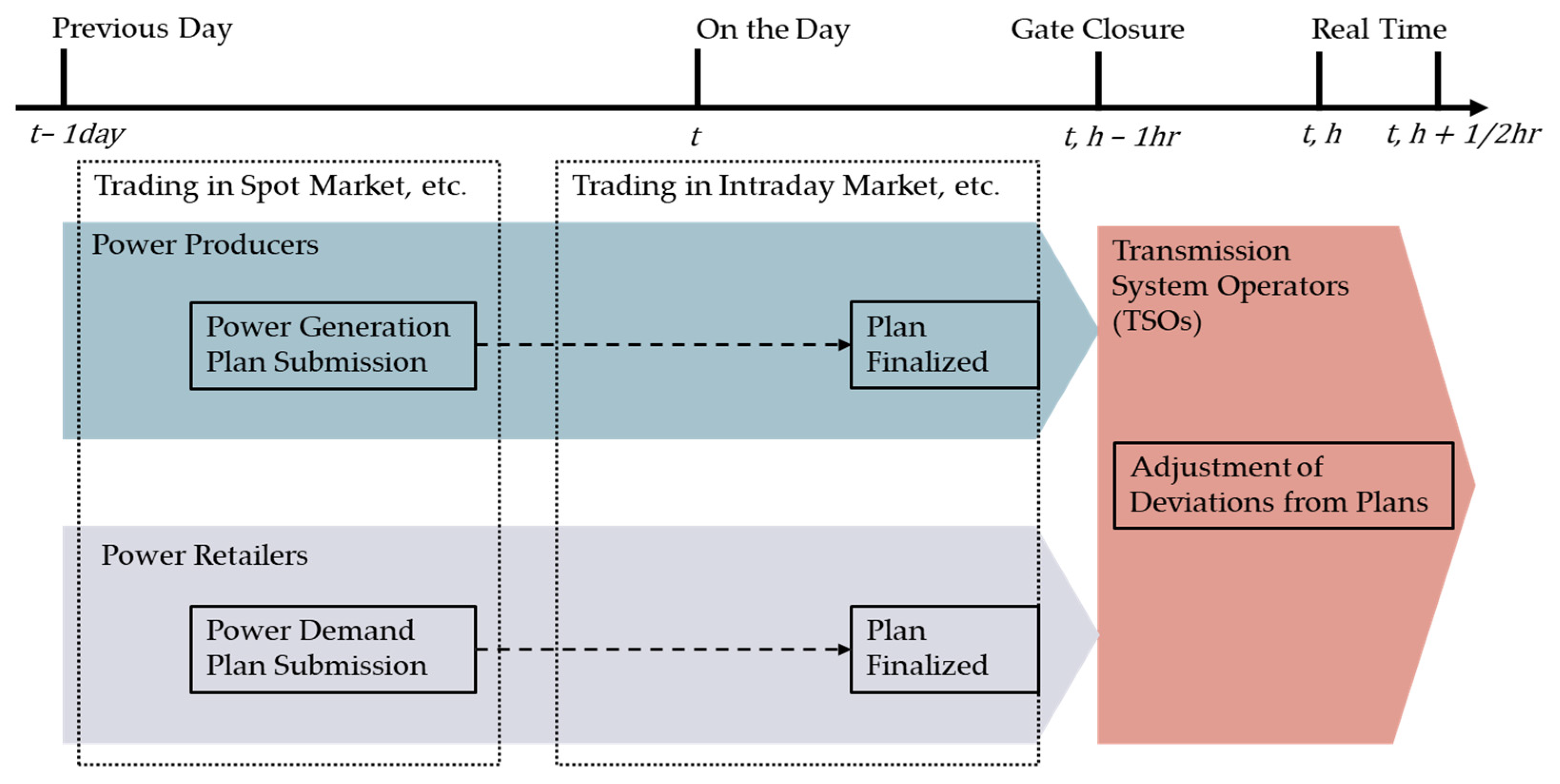
In the Japanese electricity market, the real-time balancing of supply and demand is supported by a structured timeline involving multiple stakeholders, including power producers, power retailers, and TSOs. As illustrated in Figure 1, this process begins with power producers and retailers formulating half-hourly power generation and procurement plans, which must be submitted by 12:00 noon on the previous day. These plans are designed to balance the system’s total supply and demand at the planning stage. Participants may adjust their plans up until one hour before real-time operations (Gate Closure). Despite these efforts, real-time deviations often occur between the planned and actual values in real time, due to uncertainties in renewable power generation or changes in customer demand, which are often caused by unexpected weather conditions. This leads to imbalances at the individual level. At the system level, the NIV is calculated as the algebraic sum of all individual imbalances, whereas the TSO is responsible for compensating for the gap between total supply and demand in the power system by procuring balancing resources procured from the reserve market. Therefore, the NIV can be regarded as equivalent to the supply–demand gap in the grid that needs to be compensated for by the TSO. In other words, the NIV effectively reflects the mismatch between system-wide supply and demand, which the TSO balances to maintain grid stability. Following these physical adjustments, financial settlements are conducted between the TSO and market participants based on each participant’s imbalance amount and the corresponding imbalance prices, which reflect the state of the NIV. Imbalance pricing systems can be broadly categorized into dual-pricing and single-pricing. As discussed in [21,22,26], under a dual-pricing system, separate imbalance prices are applied to surpluses and shortages depending on the state of each participant. In contrast, a single-pricing system applies a uniform price to all participants, determined by the overall system condition, as indicated by the NIV. Under a single-pricing regime, the imbalance price rises during shortages and falls during surpluses, reflecting the marginal cost of balancing the grid. This pricing mechanism encourages market participants to adjust their operations according to system conditions. Since 2022, Japan has shifted from a dual-pricing to a single-pricing system to better reflect the real-time value of electricity and the adjustment costs incurred by TSOs. This provides clearer signals and stronger incentives for market participants to balance their operations [27].

2.2. Importance of System Imbalance Signals

The NIV can be considered to be zero when no system imbalance occurs, and to be positive or negative in the case of a surplus or shortage, respectively. In this study, we define an indicator function based on the sign of the NIV (see Section 2.3 below), which takes the value 1 if the NIV is positive, and 0 if it is negative or zero. We refer to this indicator as the system imbalance signal. Under the single-pricing regime, market participants with imbalances that align with the system imbalance signal face penalties, while those with imbalances in the opposite direction are incentivized [21].

If a retail electricity provider can anticipate that the NIV will be positive (i.e., indicating a system surplus), they may regard surplus as posing a greater risk than shortage, and adjust their procurement and bidding strategies accordingly. Similarly, for solar power producers, the ability to predict the sign of the NIV in advance enables them to assess whether a surplus or shortage poses a greater financial risk and to adopt more flexible bidding strategies. Furthermore, if they own adjustable thermal units, they may benefit from incentives by helping to resolve the system imbalance while absorbing the uncertainty associated with solar power output. This suggests that power producers may enhance their revenues by strategically planning their generation schedules.

These practical scenarios illustrate how system imbalance signals play a crucial role not only in guiding TSOs to efficiently balance supply and demand, but also in helping market participants to refine their strategies in order to mitigate financial risks and align with grid conditions, ultimately contributing to system stability. Given the growing complexity of power system operations, a comprehensive understanding of the factors influencing imbalance signals—and a structured approach to their prediction—is essential to support decision-making by both market participants and TSOs.

2.3. Problem Formulation as Binary Classification

Before proceeding to the methodology and problem formulation, we note that the key notations and abbreviations used throughout this paper are summarized at the end of the paper.

This study provides a comprehensive analysis of system imbalance signals—defined as conditions of shortage or surplus in the power system. It includes both a sensitivity analysis to explore the mechanisms behind imbalance formation, and a next-day forecasting task designed to support real-world operational decision-making.

To this end, we formulate the following system imbalance signal as a binary classification problem:

$$Y_{t,h}={\mathbb{1}}_{\left\{{NIV}_{t, h}>0 \right\}}$$

(1)

In (1), the target variable $Y_{t,h}$ is derived from the observed ${NIV}_{t,h}$ at each hourly time step ($t, h$), with the binary event defined as a system surplus when ${NIV}_{t,h}>0$, or a system shortage when ${NIV}_{t,h}\le 0$.

To model this classification task, we employ ML techniques that can capture nonlinear relationships and high-dimensional interactions among features—including historical NIV data, market variables, weather information, and calendar effects. Specifically, we analyze how various explanatory variables contribute to the formation of imbalance signals, providing comprehensive insights into the underlying mechanisms. In parallel, we construct predictive models to forecast the system imbalance signal for each hourly time slot of the following day, using only information available before the spot market closure. These models can support early-stage decision-making for both market participants and TSOs under real-world operational conditions. The detailed methodological design is described in the next section.

3. Methodology

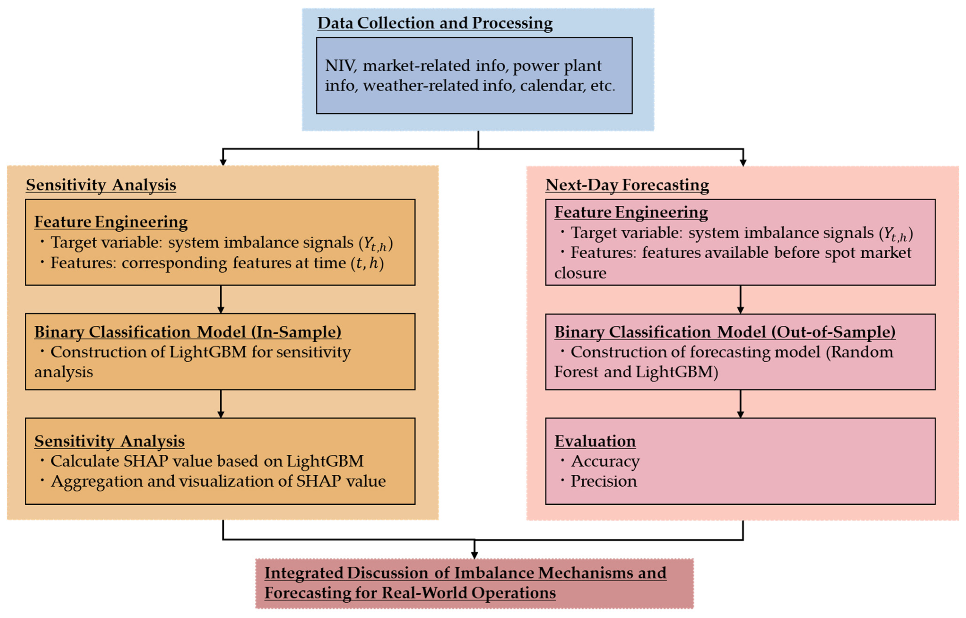
This section presents the methodological framework developed for analyzing and forecasting electricity system imbalance signals. As outlined in Figure 2, the approach comprises two complementary components: an in-sample sensitivity analysis to improve interpretability and understanding of imbalance mechanisms, and an out-of-sample next-day forecasting framework intended to support practical decision-making in real-world operations. Both components are formulated as binary classification tasks, in which the system imbalance signal is predicted based on a range of explanatory variables. The models employed are based on ML algorithms, which are well suited for capturing nonlinear relationships and high-dimensional feature interactions.

This section proceeds as follows: First, we describe the data sources and feature construction process. Then, we present the ML and eXplainable AI (XAI) techniques adopted in this study. Finally, we detail the in-sample sensitivity analysis and demonstrate the next-day forecasting methodology.

3.1. Data and Feature Preparation

This study focuses on the TEPCO region, where the power system is operated by TEPCO Power Grid, Incorporated (TEPCO Power Grid), the regional TSO headquartered in Tokyo, Japan, covering Tokyo and the surrounding prefectures: Kanagawa, Saitama, Chiba, Tochigi, Gunma, Ibaraki, and Yamanashi, as well as parts of Shizuoka. We focus on the data period from 1 April 2022 to 31 December 2024, which aligns with the implementation of Japan’s latest single-pricing imbalance settlement system and extends to the most recent available data.

Table 1 provides an overview of the datasets used in this study, including their sources and other relevant information. The core target variable is the system imbalance signal, formulated as a binary classification target. Information related to system imbalances is published on the Imbalance Prices Calculation Service (ICS) website [28]. As the granularity of the relevant features is hourly, this study uses the hourly imbalance signal as the target variable. Using the published NIV data for the TEPCO region, the ${NIV}_{t,h}$ for hour $h$ on day $t$ is calculated as the average of the two half-hourly NIV values within that hour (i.e., the values for 0–30 min and 30–60 min within the past hour $h$). As defined in Section 2.3, if the ${NIV}_{t,h}$ is positive, it is categorized as a system surplus ($Y_{th}=1$); otherwise, it is categorized as a system shortage ($Y_{th}=0$). Any missing data are interpolated using the average for the same month and hour across the dataset.

Market-related variables, including spot market prices and contract success ratios, are sourced from the Japan Electric Power Exchange (JEPX) [29]. Spot prices are similarly aggregated from half-hourly to hourly resolution. Sell-side and buy-side contract rates are calculated as the ratio of contract volume to bid volume in the spot market.

Information on thermal power plant shutdown capacity is published by the Power Generation Information Disclosure System (HJKS) [30]. These data are aggregated into daily total shutdown capacity, categorized as planned shutdowns (denoted as $x_5$), unplanned shutdowns (denoted as $x_6$), and output reductions (denoted as $x_7$).

Weather-related features serve as important explanatory variables, as they significantly affect both electricity demand and renewable power generation. Actual temperature ($x_8$) and solar radiation ($x_{11}$) data are collected from Japan Meteorological Agency (JMA) [31] at multiple locations within the TEPCO region. We selected data from JMA observatory stations in the top four prefectures with the highest electricity demand [32] and the top four prefectures with the highest solar power generation capacity [33], as detailed in

Table 2. Selected locations for weather-related data in the TEPCO region.

Observatory Stations	Prefectures	Temperature-Related	Solar Radiation-Related
Marunouchi	Tokyo	Yes	Yes
Yokohama	Kanagawa	Yes
Saitama	Saitama	Yes
Chiba	Chiba	Yes
Tsukuba	Ibaraki	Yes	Yes
Choshi	Chiba	Yes	Yes
Utsunomiya	Tochigi	Yes	Yes
Maebashi	Gunma	Yes	Yes

. Forecasted temperature ($x_9$) and solar radiation ($x_{12}$) data are based on Grid Point Value (GPV) forecasts. For this study, we extracted the data corresponding to the grid points closest to each JMA weather station, using latitude and longitude coordinates. These data were collected and distributed by the Research Institute for Sustainable Humanosphere, Kyoto University (http://database.rish.kyoto-u.ac.jp/index-e.html, accessed on 26 January 2025) [34]. The forecasts are updated four times daily, covering the next 264 h. For this analysis, we use the latest forecast published before the start of spot market trading, which is updated at 18 UTC (03 JST) each day. Forecast errors ($x_{10}$ and $x_{13}$) are calculated as the difference between actual and forecasted values to approximate deviations in load and renewable generation.

Table 1. A summary of the input features used in the modeling framework.

Data	Notation	Units	Source
NIVs	$x_1$	kWh	ICS [28]
Spot market prices	$x_2$	JPY/kWh	JEPX [29]
Sell contract rates (spot market)	$x_3$	%	JEPX [29]
Buy contract rates (spot market)	$x_4$	%	JEPX [29]
Thermal power plant shutdown capacity	$x_5–x_7$	kW	HJKS [30]
Actual temperature	$x_8$	°C	JMA [31]
Forecasted temperature	$x_9$	°C	RISH Data Server [34]
Forecast error of temperature	$x_{10}$	°C	$x_8-x_9$
Actual solar radiation	$x_{11}$	Wh	JMA [31]
Forecasted solar radiation	$x_{12}$	Wh	RISH Data Server [34]
Forecast error of solar radiation	$x_{13}$	Wh	$x_{11}-x_{12}$

Table 1. A summary of the input features used in the modeling framework.

Data	Notation	Units	Source
NIVs	$x_1$	kWh	ICS [28]
Spot market prices	$x_2$	JPY/kWh	JEPX [29]
Sell contract rates (spot market)	$x_3$	%	JEPX [29]
Buy contract rates (spot market)	$x_4$	%	JEPX [29]
Thermal power plant shutdown capacity	$x_5–x_7$	kW	HJKS [30]
Actual temperature	$x_8$	°C	JMA [31]
Forecasted temperature	$x_9$	°C	RISH Data Server [34]
Forecast error of temperature	$x_{10}$	°C	$x_8-x_9$
Actual solar radiation	$x_{11}$	Wh	JMA [31]
Forecasted solar radiation	$x_{12}$	Wh	RISH Data Server [34]
Forecast error of solar radiation	$x_{13}$	Wh	$x_{11}-x_{12}$

The above features were selected based on their relevance to the formation of system imbalance. Market-related features capture the autocorrelation of NIVs and the relationship between spot market trading and real-time power system conditions. Weather-related features, including temperature and solar radiation forecasts and their respective errors, reflect the strong impact of climate variability on both electricity demand and renewable generation. Thermal power plant shutdown capacity is included to capture localized trends in thermal generation output. Additionally, calendar-based features—such as the month, season, hour, weekends, and public holidays—are incorporated to reflect demand-side variations associated with behavioral patterns and significant social events. The feature engineering approaches used in the sensitivity analysis and next-day forecasting are described in detail in Section 3.3 and Section 3.4, respectively.

3.2. ML and XAI Techniques

This study employs the following ML and XAI techniques: RF, Light Gradient Boosting Machine (LightGBM), and SHAP. These methods were chosen for their ability to handle high-dimensional, nonlinear relationships, while offering model interpretability. While other algorithms, such as eXtreme Gradient Boosting (XGBoost), Support Vector Machines (SVMs), and DL methods, could also be effective, they were not included in this study for practical and methodological reasons. Compared to XGBoost, LightGBM offers improved training efficiency, which is discussed in Section 3.2.2. SVMs typically require careful kernel selection and are less efficient when scaling to high-dimensional feature sets. DL models require larger datasets to leverage their strengths. Given our focus on updated post-2022 data from the Japanese settlement system, the available dataset is moderate in size and not ideally suited for DL methods. Similar research has also reported that RF outperforms LSTM in imbalance forecasting, supporting the effectiveness of tree-based models in this context [15].

3.2.1. RF

RF is a tree-based ensemble learning method introduced in [35], designed to improve predictive accuracy and reduce overfitting. Unlike single decision trees, which are prone to high variance and instability, RF addresses these issues by training an ensemble of decision trees. Each tree is built from a different bootstrap sample of the original dataset—a process known as bagging—and their predictions are then aggregated. Each tree is constructed independently using a random subset of features at each split, which promotes diversity among the trees and reduces the risk of overfitting.

As illustrated in Equation (2), for classification tasks, the final prediction is acquired via majority voting across all trees:

$$\hat{y}=majority\_vote(T\_1 (x),T\_2 (x),\dots ,T\_M (x\left)\right)$$

(2)

where $T_M\left(x\right)$ denotes the prediction of the $m$-th decision tree, $M$ represents the total number of trees in the forest, and $\widehat{y}$ is the final prediction.

3.2.2. LightGBM

LightGBM is a highly efficient ML framework introduced in [36]. It is based on the concept of Gradient Boosting Decision Trees (GBDTs), which combines decision trees, boosting, and Gradient-based optimization to iteratively improve predictions. At its core, LightGBM applies Gradient Boosting, a sequential ensemble learning method where each new decision tree (weak learner) is trained to correct the residual errors of the previous models. This iterative process minimizes a predefined loss function (4) and gradually improves model performance over time. The final prediction is the sum of predictions from all M weak learners (trees), as shown in (3):

$$\widehat{y}=\sum _{m=1}^M{T}_m\left(x\right)$$

(3)

where $T_m\left(x\right)$ denotes the prediction of the $m$-th decision tree, $M$ represents the total number of trees in the ensemble, and $\widehat{y}$ is the final prediction.

LightGBM uses Gradient-based optimization to adjust predictions, ensuring the loss function is minimized over time. The model is trained by minimizing a specified loss function ($L$), which guides the learning process. The loss function can be expressed as follows:

$$L=\sum _{i=1}^{n}l\left(y_i, {\widehat{y}}_i\right)+\sum _{m=1}^M\Omega \left(f_m\right)$$

(4)

where $l\left(y_i, {\widehat{y}}_i\right)$ denotes the loss between the true value $y_i$ and the predicted value ${\widehat{y}}_i$, $\Omega \left(f_m\right)$ is a regularization term applied to the m-th tree to prevent overfitting, $n$ is the number of data instances, and $M$ represents the total number of decision trees (weak learners) in the ensemble.

At each iteration, LightGBM uses the Gradients ($g_i$) and Hessians ($h_i$) calculated from the loss function to build new decision trees as weak learners that minimize the residual errors. These Gradients and Hessians are defined as follows:

$$g_i={\displaystyle \frac{\mathsf{\partial }l}{\mathsf{\partial }{\widehat{y}}_i}}, h_i={\displaystyle \frac{{\mathsf{\partial }}^{2}l}{\mathsf{\partial }{\widehat{y}}_i^2}}$$

(5)

This iterative process ensures that each subsequent tree contributes to reducing the overall loss, improving the model’s predictions. LightGBM is designed for efficiency and scalability, making it ideal for large datasets. Its key features include the following:

• Leaf-wise Tree Growth: LightGBM grows trees leaf-wise by splitting the leaf with the greatest potential for reducing loss. This approach leads to deeper and more accurate trees compared to level-wise growth, while maintaining efficiency.
• Histogram-based: Continuous features are bucketed into discrete bins, which significantly reduces memory usage and accelerates split finding.
• Gradient-based One-Side Sampling (GOSS): GOSS prioritizes samples with larger Gradients (indicating higher prediction error) during split calculations, enabling efficient training without significantly compromising model accuracy.

3.2.3. SHAP

SHAP is a unified framework for interpreting ML model predictions, introduced in [37]. It is grounded in Shapley values from cooperative game theory, enabling SHAP to fairly allocate the contribution of each input feature to a model’s output. In the context of ML, SHAP assigns importance values to individual features to explain their respective impact on prediction results. It has been widely applied across various fields, including demand-related analysis in the energy sector, where it has been recognized as a valuable tool for interpreting the influence of input variables on model outputs [38,39,40].

Derived from cooperative game theory, Shapley values fairly distribute the total gain (or cost) among players (features) based on their individual contributions. As shown in (6), the Shapley value for feature $j$ is defined as follows:

$${\varphi }_j=\sum _{S\subseteq F\setminus \left\{j\right\}}{\displaystyle \frac{\left|S\right|!\left(\left|F\right|-\left|S\right|-1\right)!}{\left|F\right|!}}\left[f\left(S\cup \left\{j\right\}\right)-f\left(S\right)\right]$$

(6)

where $F$ is the full set of input features, $S$ is a subset of features excluding feature $j$, $f\left(S\right)$ is the model output when only features in subset $S$ are used, and ${\varphi }_j$ represents the marginal contribution of feature $j$ averaged over all possible subsets.

With the additive property of SHAP as shown in (7), the model’s output can be decomposed into a sum of contributions from individual features:

$$\widehat{y}={\varphi }_0+\sum _{j=1}^d{\varphi }_j{(x}_j)$$

(7)

where $\widehat{y}$ is the model’s output, ${\varphi }_0$ is the base value (expected prediction for a baseline instance), and ${\varphi }_j{(x}_j)$ is the SHAP value for feature $j$, representing its contribution to the model’s output given input $x_j$.

3.3. Construction of Sensitivity Analysis Using LightGBM and SHAP

A binary classification model was constructed using LightGBM, trained to classify hourly system imbalance signals by distinguishing between surplus and shortage conditions. Furthermore, SHAP was applied to this model to quantify the contribution of each feature to the model’s output (surplus or shortage), enabling an in-depth analysis of the factors driving imbalances.

The target variable was the system imbalance signal for hour $h$ on day $t$, as defined in Section 2.3. The explanatory variables were categorized as follows:

• Lagged NIV ($x_1$, as denoted in Table 1): the system NIV for the same time slot from the previous day to seven days prior ($x_{1,t-1,h}–x_{1,t-7,h}$);
• Market-related features ($x_2–x_4$, as denoted in Table 1): the spot market prices and contract rates for the same time slot on the same day ($x_{2,t,h}$, $x_{3,t,h}$, $x_{4,t,h}$);
• Thermal power plant shutdown capacity ($x_5–x_7$ denoted in Table 1): the thermal power plant shutdown capacity for the same time slot on the same day ($x_{5,t,h}$, $x_{6,t,h}$, $x_{7,t,h}$);
• Weather-related features ($x_8$, $x_{10}$, $x_{11}$, $x_{13}$, as denoted in Table 1): the actual temperature and solar radiation for the same time slot on the same day, along with their forecast errors ($x_{8,t,h}$, $x_{10,t,h}$, $x_{11,t,h}$, $x_{13,t,h}$);
• Calendar-related features: the month (1–12), seasonal dummy variables (summer, autumn, winter), hour of the day (0–23), and dummy variables for weekends and public holidays.

To construct the LightGBM model, hyperparameters that significantly influenced model accuracy were optimized. The validation period spanned from 1 October 2023 to 31 December 2024. During this period, a time-series cross-validation approach was applied: for each validation month, the training data consisted of all data from April 2022 up to the month immediately preceding the validation month. Then, model performance was evaluated based on the validation month, and the set of hyperparameters that minimized validation errors across all months was selected. Using these optimal hyperparameters, the final LightGBM model was retrained on the full dataset from 1 April 2022 to 31 December 2024. This ensured that the training and validation sets were chronologically separated to prevent data leakage, and that hyperparameter selection was based on robust performance across all validation months, rather than isolated peak performance.

In this binary classification task, the output of the LightGBM model represents the probability that the imbalance signal is a surplus (i.e., $Y_{th}=1$). SHAP values ${\varphi }_j{(x}_j)$ indicate how much the $j$-th feature with input $x_j$ contributes to deviating the model’s output from the baseline prediction. Specifically, a feature contributes to a surplus prediction if its SHAP value is positive; otherwise, it contributes to a shortage. SHAP values are then aggregated and visualized to identify the most influential features and the direction of their impact.

3.4. Construction of Next-Day Forecasting Using LightGBM and RF

We constructed a next-day forecasting framework for system imbalance signals, designed to provide practical and actionable insights for real-world operations in electricity markets. The forecasting process was developed with a focus on real-world constraints, ensuring its applicability in actual operational settings.

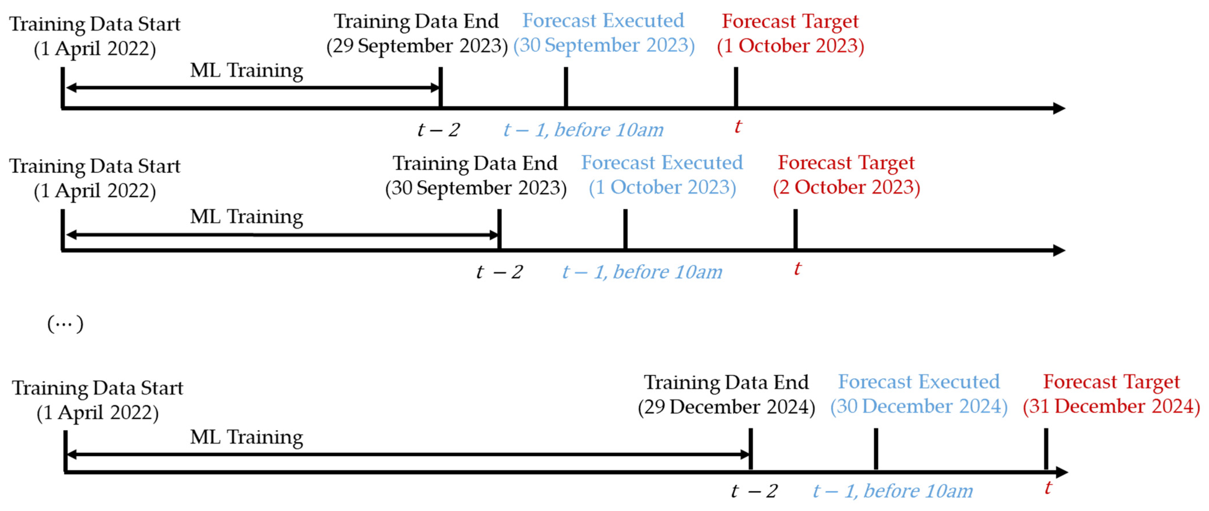
Figure 3 shows the timeline for executing the daily forecast. To evaluate the usefulness of the proposed approach, the test period covered 1 October 2023 to 31 December 2024. This period covered over one year of recent market conditions, providing a robust basis for assessing the model’s performance under varying conditions. For each day $t$ in the test period, the forecast was executed on day $t-1$, prior to the closure of the spot market. The training dataset included only historical data available from 1 April 2022 up to day $t-2$, ensuring that the ML model was trained using information accessible at the time of forecast execution. To improve the forecasting models, we applied a time-series cross-validation approach using the TimeSeriesSplit function from scikit-learn, with three splits. In this approach, the training data were sequentially split into growing training sets and forward-looking validation sets. For each split, the model was trained using earlier data and validated using the next chronological set. This ensured that validation was always performed using future data, thus avoiding data leakage. Hyperparameter tuning was conducted using the Python Optuna package 4.3.0 [41], a hyperparameter optimization framework, with 20 trials. The best hyperparameters were selected based on robust performance across all validation splits, in order to enhance model credibility and reduce the risk of overfitting. Using the trained model with the selected hyperparameters, the final forecast for each day $t$ was generated.

Two ML models—RF and LightGBM, as introduced in Section 3.2—were adopted in the forecasting framework. Based on insights from the sensitivity analysis, several feature categories were identified as critical for forecasting. These included the lagged NIV, calendar-related features, and weather-related features. However, due to operational constraints, certain data—such as the weather-related forecast errors for day $t$—were not available at the time of forecast execution on day $t-1$. To address this limitation, two different feature engineering strategies were implemented.

The first pattern (Pattern 1) used recent lagged values, such as the following:

• Lagged NIV ($x_1$, as denoted in Table 1): the NIV from the same time slot at $t-2, t-3$;
• Market-related features ($x_2–x_4$, as denoted in Table 1): the spot market prices and contract rates from the same time slot at $t-1, t-2, t-3$;
• Thermal power plant shutdown capacity ($x_5–x_7$, as denoted in Table 1): the thermal power plant shutdown capacity from the same time slot on the same day ($t$);
• Weather-related features ($x_9$, $x_{10}$, $x_{12}$, $x_{13}$, as denoted in Table 1): the forecasted values of temperature and solar radiation at $t$, along with their forecast errors from the same time slot at $t-2, t-3$;
• Calendar-related features: the month (1–12), seasonal dummy variables (summer, autumn, winter), hour of the day (0–23), dummy variables for 3 h categories, such as Hour 3–6 and Hour 7–9, and dummy variables for weekends and public holidays.

The second pattern (Pattern 2) relied on statistical summaries of recent data, such as the mean, standard deviation, minimum and maximum:

• Lagged NIV ($x_1$, as denoted in Table 1): statistical summaries of the NIV for the same slot, from $t-2$ to $t-14$;
• Market-related features ($x_2–x_4$, as denoted in Table 1): statistical summaries of spot market prices and contract rates for the same time slot, from $t-1$ to $t-14$;
• Thermal power plant shutdown capacity ($x_5–x_7$ denoted in Table 1): the thermal power plant shutdown capacity from the same time slot on the same day ($t$);
• Weather-related features ($x_9$, $x_{10}$, $x_{12}$, $x_{13}$, as denoted in Table 1): forecasted values of temperature and solar radiation at $t$, along with statistical summaries of their forecast errors for the same time slot, from $t-2$ to $t-14$;
• Calendar-related features: the same as for Pattern 1.

Further consideration was required for weather-related features, due to the spatial variability in weather conditions across the TEPCO region. To account for these, three configurations of weather-related features were explored:

(a)

The first configuration used data exclusively from Marunouchi (Tokyo), which represents the largest demand center in the region.

(b)

The second configuration combined data from Marunouchi (Tokyo) and Tsukuba (Ibaraki), as these areas are characterized by the highest demand or highest penetration of solar power generation in the TEPCO region.

(c)

The third configuration expanded the scope to include data from eight locations: Marunouchi (Tokyo), Yokohama (Kanagawa), Saitama (Saitama), Chiba (Chiba), Tsukuba (Ibaraki), Choshi (Chiba), Utsunomiya (Tochigi), and Maebashi (Gunma), as these locations are top four with the highest electricity demand and the top four with the highest solar power generation capacity.

Each combination of ML model, feature engineering strategy, and weather data configuration is systematically labeled in

Table 3. Notation for different forecast model configurations.

Feature Engineering	Weather Data	RF	LightGBM
1	(a)	RF1	LGBM1
1	(b)	RF2	LGBM2
1	(c)	RF3	LGBM3
2	(a)	RF4	LGBM4
2	(b)	RF5	LGBM5
2	(c)	RF6	LGBM6

.

3.5. Performance Metrics

To evaluate the performance of the classification models constructed in Section 3.3 and Section 3.4, three metrics were used: $Accuracy$, ${Precision}_{surplus}$, and ${Precision}_{shortage}$. These metrics provided a balanced evaluation of the models’ performance across the two classes, ensuring reliable results even in the presence of class imbalance.

$Accuracy$ indicates the proportion of correct predictions across all forecasts during the target evaluation period, and is defined as follows:

$$Accuracy={\displaystyle \frac{1}{T\times H}}\sum _{t=1}^T\sum _{h=0}^H{\mathbb{1}}_{\left\{Y_{t,h}={\widehat{y}}_{t,h} \right\}}$$

(8)

where $t\in \left\{1,2,\dots ,T\right\}$ and $h\in \left\{0,1,\dots ,H\right\}$ denote the day and hour indices, with $H+1 \left(=24\right)$ total hours per day. For the sensitivity analysis, $T$ spans the date range from 1 April 2022 to 31 December 2024, as described in Section 3.3. For the next-day forecasting evaluation, $T$ covers 1 October 2023 to 31 December 2024 as explained in Section 3.4.

While $Accuracy$ provides an overall measure of performance, it may not fully capture the model’s effectiveness for individual classes, especially in imbalanced datasets.

$Precision$ represents the proportion of instances predicted as surplus or shortage that are actually surplus or shortage, respectively. It is defined separately for each class, as follows:

$$\begin{gathered} {Precision}_{surplus}={\displaystyle \frac{{\sum }_{t=1}^T{\sum }_{h=0}^H{\mathbb{1}}_{\left\{Y_{t,h}={\widehat{y}}_{t,h}=1 \right\}} }{{\sum }_{t=1}^T{\sum }_{h=0}^H{\mathbb{1}}_{\left\{{\widehat{y}}_{t,h}=1 \right\}}}}, \\ {Precision}_{shortage}={\displaystyle \frac{{\sum }_{t=1}^T{\sum }_{h=0}^H{\mathbb{1}}_{\left\{Y_{t,h}={\widehat{y}}_{t,h}=0 \right\}}}{{\sum }_{t=1}^T{\sum }_{h=0}^H{\mathbb{1}}_{\left\{{\widehat{y}}_{t,h}=0 \right\}}}} \end{gathered}$$

(9)

All model training and evaluation were conducted using the high-memory runtime and NVIDIA T4 GPU environment provided by Google Colab. All models were implemented in Python 3.11, using the LightGBM and scikit-learn libraries for model construction and the SHAP library for SHAP analysis. All results presented in Section 4 and Section 5 were generated using this setup, following the methodology described in Section 3.3, Section 3.4 and Section 3.5.

4. Sensitivity Analysis Results and Feature-Specific Insights

This section presents the results of the sensitivity analysis conducted using SHAP, based on the LightGBM model constructed in Section 3.3. The analysis aims to identify the key features that contribute to the formation of system imbalance signals, providing an interpretable overview of the relative importance and directional influence of explanatory variables over time and in different regions. The LightGBM model achieved $Accuracy=0.93$, ${Precision}_{shortage}=0.92$, and ${Precision}_{surplus}=0.94$. These results suggest that the model is capable of classifying both shortage and surplus imbalances in a balanced manner, providing a reliable foundation for conducting the sensitivity analysis.

4.1. Hourly Trends of Feature Contributions

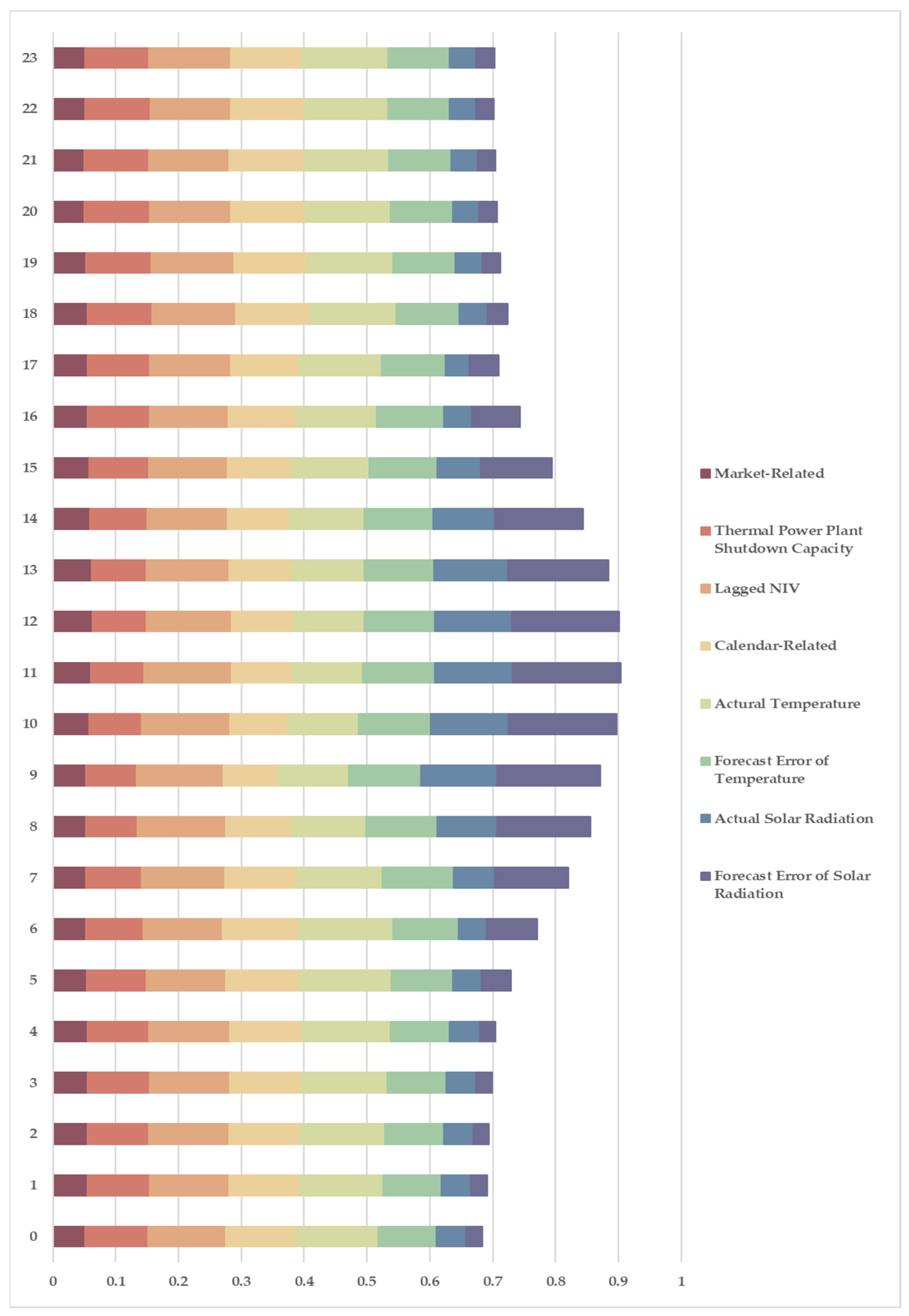
We first examine the hourly trends of feature contributions derived from the SHAP analysis. Figure 4 illustrates the average absolute SHAP values, grouped by feature categories for each hour of the day. The horizontal bars represent the aggregated importance of each feature category, as defined in Section 3.3, and offer insights into how various factors contribute to the model’s predictions. The results reveal clear temporal variations, with certain features dominating at different times of the day, reflecting the dynamic nature of imbalance drivers. Specifically, temperature-related and calendar-related features tend to be more influential from the evening through the early-morning hours, while solar radiation-related features play a central role during the daytime. In addition, the lagged NIV consistently exhibits strong importance throughout the day, underscoring its reliability as a predictor of imbalance.

These patterns can be attributed to the underlying dynamics of electricity demand and supply. During night-time and early-morning hours, residential consumption patterns dominate, driven by routine human activities and weather-dependent heating or cooling demands. Consequently, temperature becomes a major contributing factor. Calendar-related variables such as weekends and public holidays further modulate these patterns by introducing variations in demand over time.

In contrast, daytime imbalances are significantly influenced by fluctuations in solar power generation, which increase the variability of renewable energy supply. Forecast errors in solar radiation further highlight the difficulty of accurately managing renewable sources, as even slight deviations from the expected output can cause significant imbalances in the system. The persistent importance of lagged NIV across all time slots suggests that imbalance signals exhibit strong temporal autocorrelation, reflecting recurring patterns and continuity in power system dynamics.

4.2. Regional Variation in Weather-Related Feature Contributions

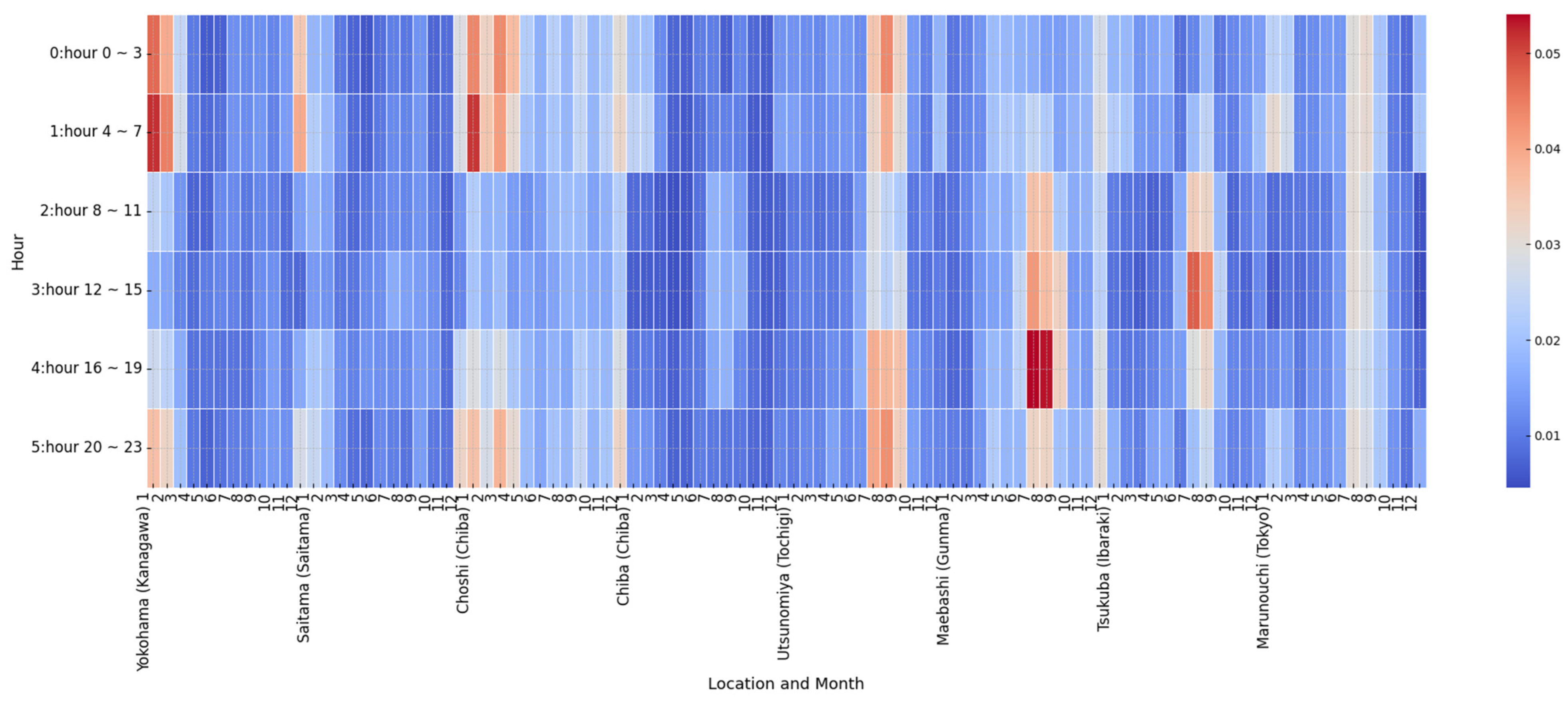
Next, we focus on the contributions of weather-related features and their regional variations, as these are among the most influential factors affecting electricity demand and renewable power generation. Figure 5 highlights the seasonal variations in the importance of temperature-related features, showing that these features are more important during the winter and summer months. These periods correspond to temperature extremes that drive the need for heating and cooling, making temperature a critical factor in explaining variations in electricity demand. The impact is less pronounced during transitional seasons such as spring and autumn, when temperature-related electricity usage tends to stabilize. These seasonal fluctuations in demand—strongly influenced by temperature—ultimately contribute to system imbalances by increasing uncertainty in usage patterns.

Notable spatial patterns emerge when examining different geographic locations. Although Tokyo exhibits the highest electricity demand within the TEPCO region, temperature-related features appear to be less important in this area. This may be due to the specific data source used—Marunouchi (Tokyo)—which likely represents an office district. Office areas tend to have relatively stable and less temperature-sensitive demand, particularly in the evening, when residential temperature-driven consumption peaks in other regions.

In contrast, regions such as Yokohama (Kanagawa), Maebashi (Gunma), and Utsunomiya (Tochigi) exhibit higher SHAP values for temperature-related features at certain times of day, especially in the early-morning and evening. These patterns reflect a stronger influence of temperature on residential demand in these areas. Each of these locations is a population center within its respective prefecture in the TEPCO region, making their demand profiles more representative of residential consumption behavior. These findings underscore the crucial interplay between temperature-driven demand variability and system imbalances. They emphasize the importance of incorporating both seasonal and regional factors in electricity grid forecasting and management.

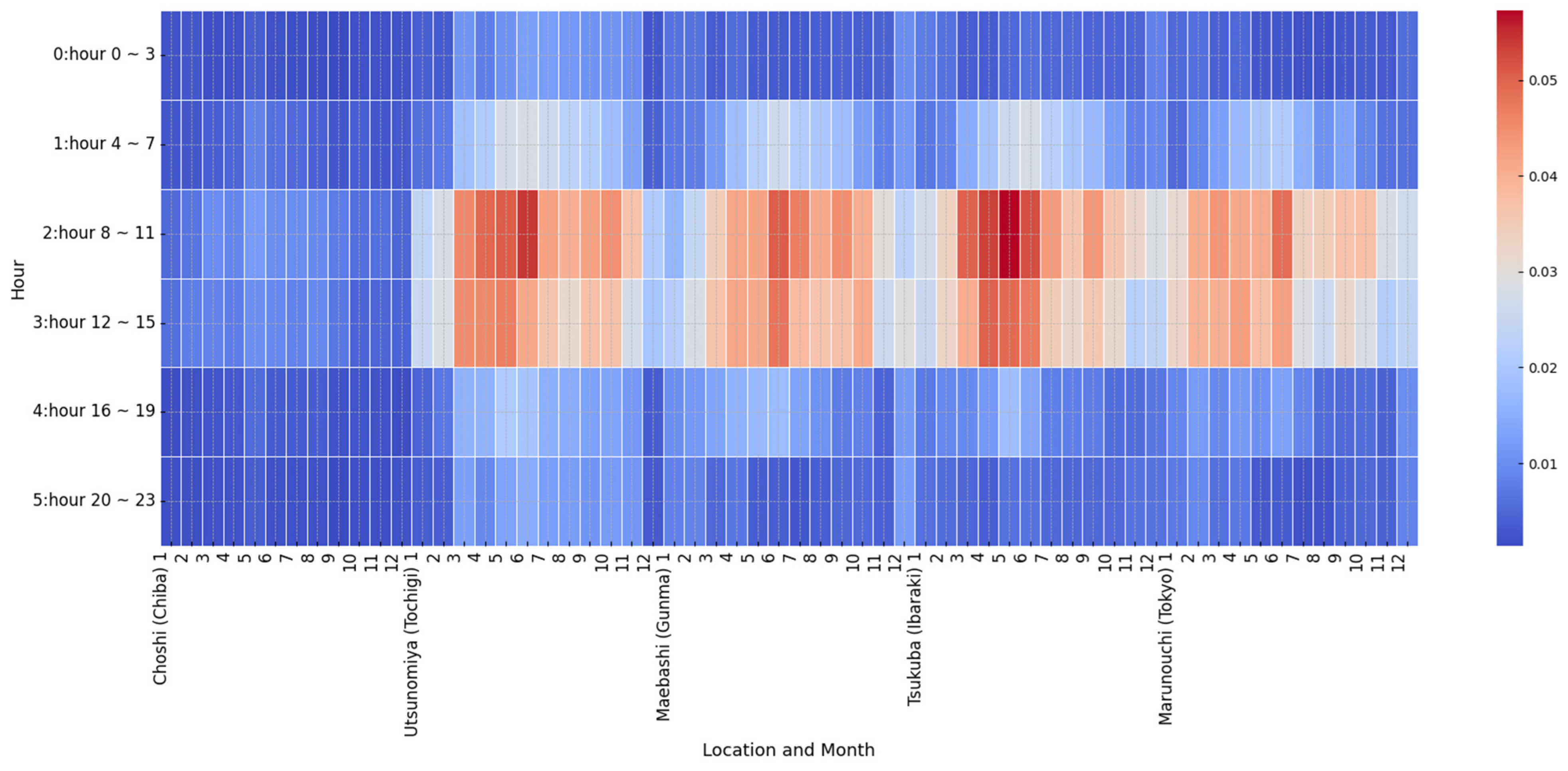
Figure 6 illustrates the average absolute SHAP values for solar radiation forecast errors across different hours, months, and locations. The results show that Ibaraki, the prefecture with the highest level of solar power penetration in the TEPCO region, exhibits the highest feature importance. This is particularly evident during daylight hours in the spring months, when solar power generation peaks and forecast errors can significantly contribute to system imbalances. Chiba and Tochigi, which have comparable levels of solar power penetration, demonstrate contrasting patterns. The data from Tochigi more effectively capture the variability in solar power generation and its influence on system imbalances, suggesting that they may be a more representative indicator of solar activity.

In contrast, the observed SHAP values for Tokyo are high during the late-spring to early-summer months. This may reflect interactions between rising solar radiation and temperature-sensitive electricity demand, rather than the effects of direct solar power generation. Tokyo’s data point likely corresponds to an urban or office district, where solar generation is limited, but demand intensifies during periods of high radiation.

These findings emphasize the importance of accounting for regional differences in both solar power penetration and the representativeness of meteorological data when analyzing the interplay between solar generation, forecast errors, and power system imbalances. A deeper understanding of these regional dynamics is essential for improving forecasting accuracy and mitigating the risks of imbalance in power systems with a high share of renewable energy.

4.3. Nonlinear Relationships and Feature Interactions

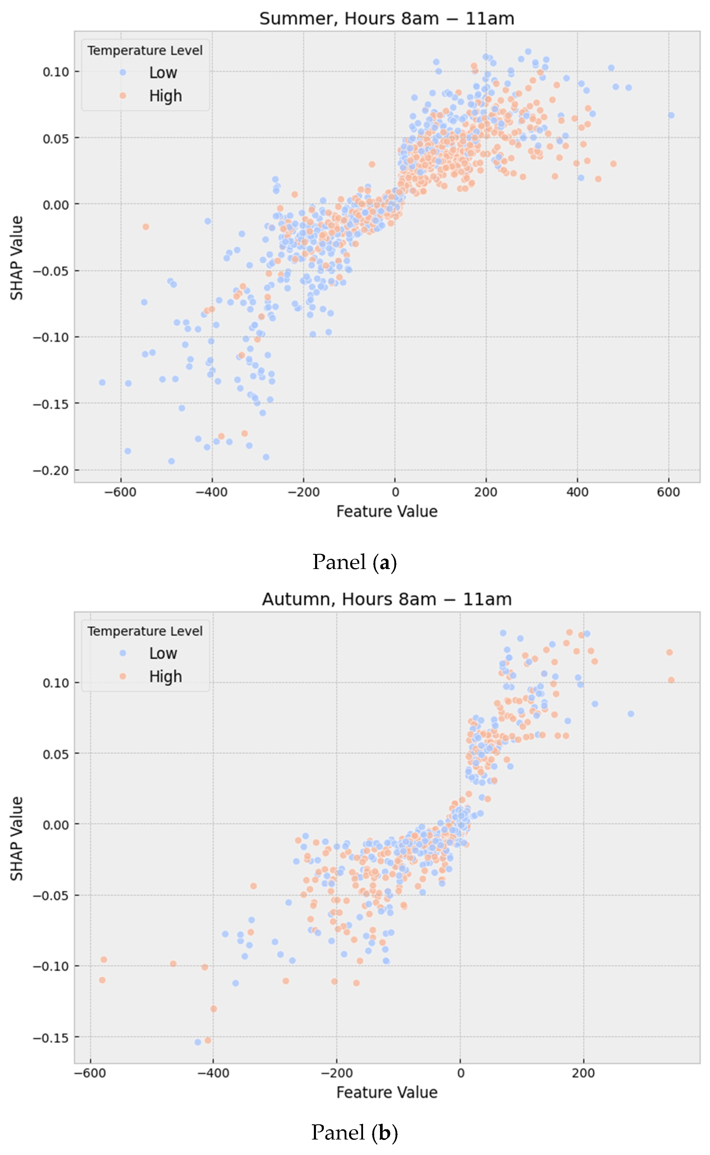
Finally, we present how feature-specific effects contribute to the occurrence of system imbalance. We use the solar radiation forecast error as an illustrative example, given its inherent uncertainty and critical role in renewable energy production. Figure 7 illustrates the relationship between the feature value of solar radiation forecast error from Tsukuba (Ibaraki) and the corresponding SHAP values during the summer (Panel (a)) and autumn (Panel (b)) seasons for hours 8 to 11. In summer (Panel (a)), the relationship is approximately linear: surplus imbalances are more likely when solar radiation exceeds the forecast (i.e., positive forecast errors), while shortage imbalances tend to occur when solar radiation falls short of the forecast (i.e., negative forecast errors). However, a notable difference emerges based on temperature levels. Higher temperatures (orange points) are associated with relatively low SHAP values, even for the same level of positive forecast error. This indicates a reduced likelihood of surplus imbalance, which can be attributed to increased electricity demand under high-temperature conditions—offsetting the surplus caused by excess solar power generation.

In contrast, the autumn scenario (Panel (b)) exhibits a nonlinear relationship. Positive forecast errors again increase the likelihood of surplus imbalance, but negative errors do not strongly correlate with shortage imbalance. This asymmetric effect may be due to the fact that electricity demand is lower overall during autumn, meaning that the surplus due to overgeneration has a more pronounced impact, while demand shortfalls are less critical.

These findings highlight the complexity of system imbalance signals, which are driven by a variety of interacting factors that exhibit different temporal and spatial characteristics. Weather-related features such as temperature and solar radiation demonstrate significant seasonal and regional variability, influencing both electricity demand and renewable energy generation. Nonlinear effects and mutual interactions between variables are also evident, underscoring the multifaceted nature of imbalance formation. Based on these insights, the next section presents the development and evaluation of next-day forecasting models for imbalance signals. By incorporating the key findings from the sensitivity analysis, these models aim to improve predictive performance and provide practical tools for real-world grid operations.

5. Next-Day Forecasting Results and Comparative Analysis

This section presents the results of next-day system imbalance signal forecasting using the LightGBM and RF models constructed in Section 3.4. Model performance is evaluated across various feature engineering patterns and weather data configurations, focusing on classification accuracy and class-wise precision under realistic operational constraints.

5.1. Overall Forecasting Performance Across the Models

We first evaluate the overall forecasting performance of all the constructed models using the metrics of $Accuracy$, ${Precision}_{shortage}$, and ${Precision}_{surplus}$, defined in Section 3.5, considering the impacts of different feature engineering patterns and weather data coverage.

As summarized in

Table 4. Performance metrics of forecast models for next-day system imbalance prediction.

Forecast Model	$\mathit{A}\mathit{c}\mathit{c}\mathit{u}\mathit{r}\mathit{a}\mathit{c}\mathit{y}$	${\mathit{P}\mathit{r}\mathit{e}\mathit{c}\mathit{i}\mathit{s}\mathit{i}\mathit{o}\mathit{n}}_{\mathit{S}\mathit{h}\mathit{o}\mathit{r}\mathit{t}\mathit{a}\mathit{g}\mathit{e}}$	${\mathit{P}\mathit{r}\mathit{e}\mathit{c}\mathit{i}\mathit{s}\mathit{i}\mathit{o}\mathit{n}}_{\mathit{S}\mathit{u}\mathit{r}\mathit{p}\mathit{l}\mathit{u}\mathit{s}}$
RF1	0.635	0.629	0.643
RF2	0.632	0.626	0.641
RF3	0.630	0.622	0.641
RF4	0.628	0.627	0.630
RF5	0.635	0.632	0.640
RF6	0.639	0.632	0.649
LGBM1	0.626	0.616	0.641
LGBM2	0.624	0.614	0.638
LGBM3	0.614	0.594	0.653
LGBM4	0.630	0.629	0.632
LGBM5	0.629	0.628	0.630
LGBM6	0.630	0.627	0.635

Note: The values highlighted in color represent the best performance in each metric across all models.

, all models achieve an $Accuracy$ exceeding 0.6, indicating strong performance in next-day forecasting. The well-balanced $Precision$ values for both shortage and surplus classes suggest that the models can predict system imbalances effectively in both directions, providing a reliable foundation for operational decision-making. Among all models, RF6 achieves the highest overall $Accuracy$, at 0.639, while RF6 and LGBM3 outperform others in class-specific precision, with RF6 achieving the highest ${Precision}_{shortage}$, at 0.632, and LGBM3 achieving the highest ${Precision}_{surplus}$, at 0.653. A key finding is that models incorporating broader weather information—specifically, data from eight locations with high electricity demand and solar power penetration—consistently outperform those relying solely on Tokyo data. This result is consistent with the sensitivity analysis, where spatial diversity in weather-related features such as solar radiation and temperature was shown to be a critical determinant of imbalance signals. The strong performance of LGBM3 and RF6 underscores the importance of capturing regional variation in weather conditions. This finding suggests that system imbalances are influenced not only by local conditions, but also by the interaction of multiple regional weather patterns.

Examining the impact of feature engineering patterns reveals a clear trend in model performance. Models based on lagged features (Feature Engineering Pattern 1: RF1–3, LGBM1–3) demonstrate higher ${Precision}_{surplus}$, whereas models using statistical summaries (Feature Engineering Pattern 2: RF4–6, LGBM4–6) achieve superior overall accuracy and higher ${Precision}_{shortage}$. These results suggest that recent lagged data are more effective in capturing short-term fluctuations, which are critical for identifying surplus events. Conversely, statistical summaries help to smooth out noise and stabilize the prediction process, thereby improving both the accuracy and precision of shortage forecasts.

Overall, the findings highlight a trade-off between temporal resolution and forecast stability. While lagged features offer signals with a high level of detail that are useful for detecting sudden variations in surplus, statistical summary-based features contribute to model robustness and reliability, particularly when forecasting shortage events. This underscores the importance of combining well-designed feature representations with spatially diverse weather data to optimize predictions of next-day system imbalances.

5.2. Comparative Insights into Shortage and Surplus Precision Compared to Baseline

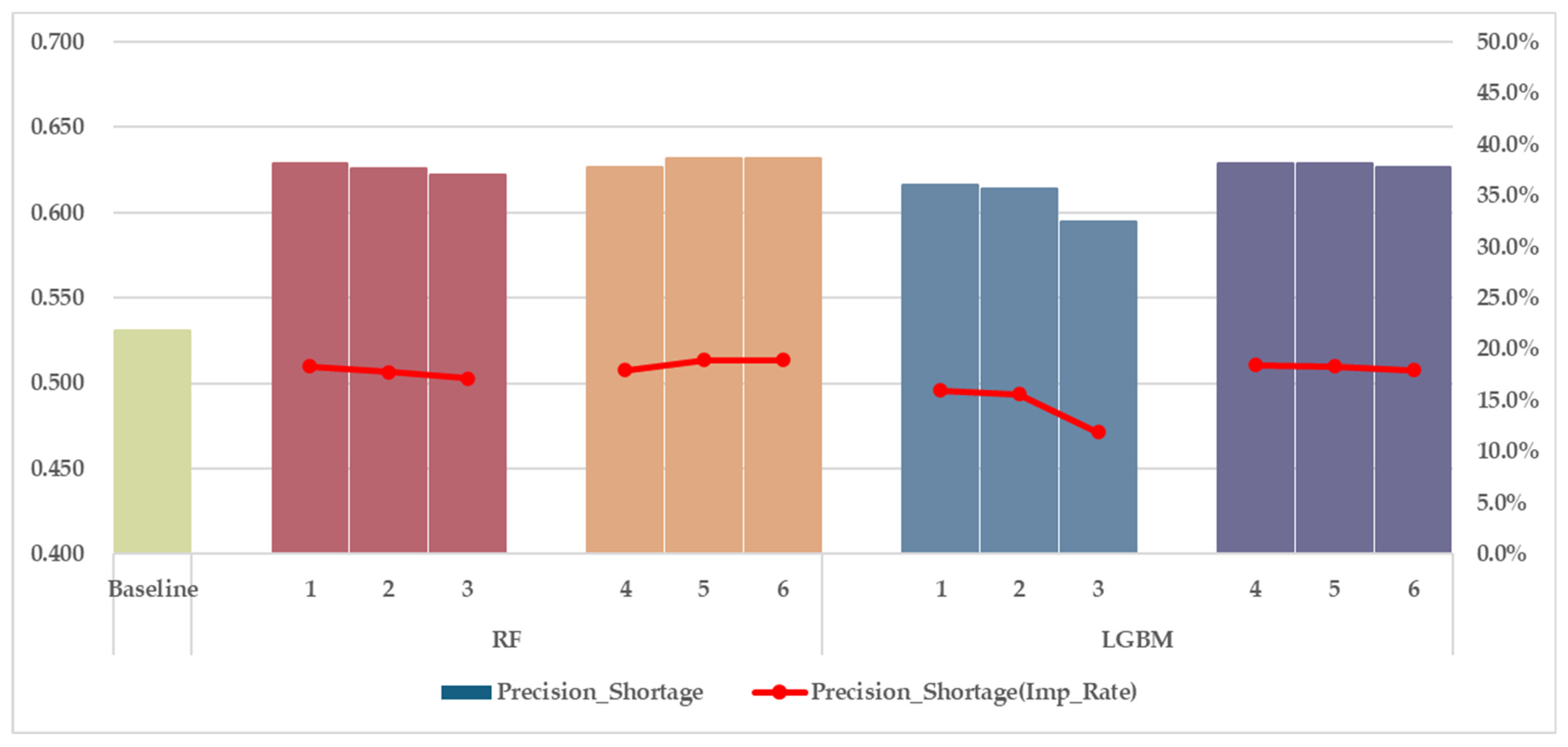
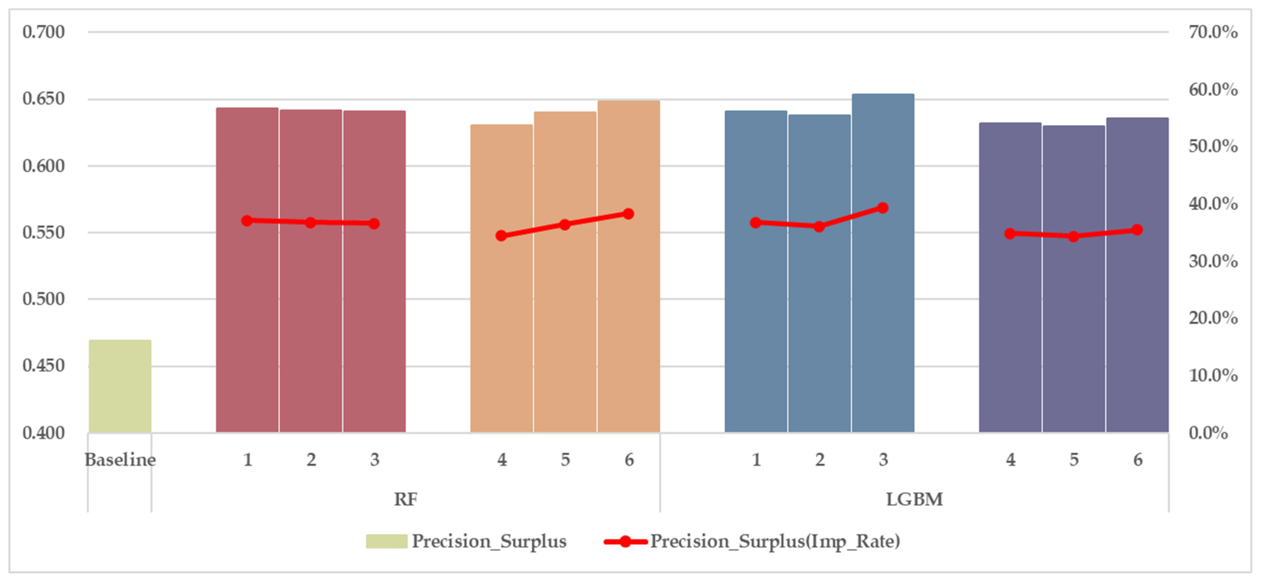
Next, we discuss insights into the forecasting performance of shortage and surplus events by comparing ${Precision}_{shortage}$ and ${Precision}_{surplus}$ against a baseline.

Figure 8 and Figure 9 summarize this comparison, where the baseline represents the expected precision if events were predicted at random based on historical trends. The baseline for each class is derived from the observed shortage and surplus ratios in the initial training period (from 1 April 2022 to 30 September 2023). The bar charts show the precision scores for each model, while the line graphs illustrate the improvement rates compared to the baseline, calculated as $(Precision-Baseline)/Baseline$.

Across both classes, all models significantly outperform the baseline, confirming that RF and LightGBM provide meaningful predictive power beyond historical trends. The precision improvement rates vary based on feature engineering approaches and weather data coverage. Models trained with lagged features (RF1–3 and LGBM1–3) tend to achieve higher ${Precision}_{surplus}$, whereas models using statistical summaries (RF4–6 and LGBM4–6) show better ${Precision}_{shortage}$. This suggests that recent lagged imbalance signals provide stronger predictive power in identifying short-term surplus events, while statistical summaries, by smoothing out noise, enhance overall model stability and improve precision in shortage classification, as previously discussed.

The impact of weather data coverage on classification performance varies between shortage and surplus events. For classification of shortages, wider weather data coverage contributes more to models based on statistical summaries (RF4–6) than those based on lagged features. This suggests that, for shortage events, incorporating aggregated weather information from multiple locations makes statistical summary models particularly effective at capturing broader imbalance trends. However, for surplus classification, the benefit of wider weather data coverage is observed in almost all models. This highlights that surplus events are more strongly influenced by diverse spatial weather conditions, such as regional solar radiation and temperature variations, which directly impact supply–demand imbalances. The best-performing models in terms of class-specific precision are LGBM3 for surplus (${Precision}_{surplus}=0.653$) and RF6 for shortage (${Precision}_{shortage}=0.632$). The strong performance of LGBM3 and RF6 reinforces the importance of capturing regional weather diversity, and highlights that the classification mechanisms for shortage and surplus events may be influenced by different factors.

In summary, the results confirm that lagged imbalance features and multi-location weather data significantly improve ${Precision}_{surplus}$, while statistical summary-based features enhance stability and improve ${Precision}_{shortage}$. The findings further validate the role of spatially diverse weather data in improving forecast precision, particularly for surplus events, aligning with the insights from the sensitivity analysis. These results reinforce the necessity of incorporating regional weather coverage in electricity imbalance prediction, while recognizing that the classification dynamics of shortage and surplus events are not completely identical.

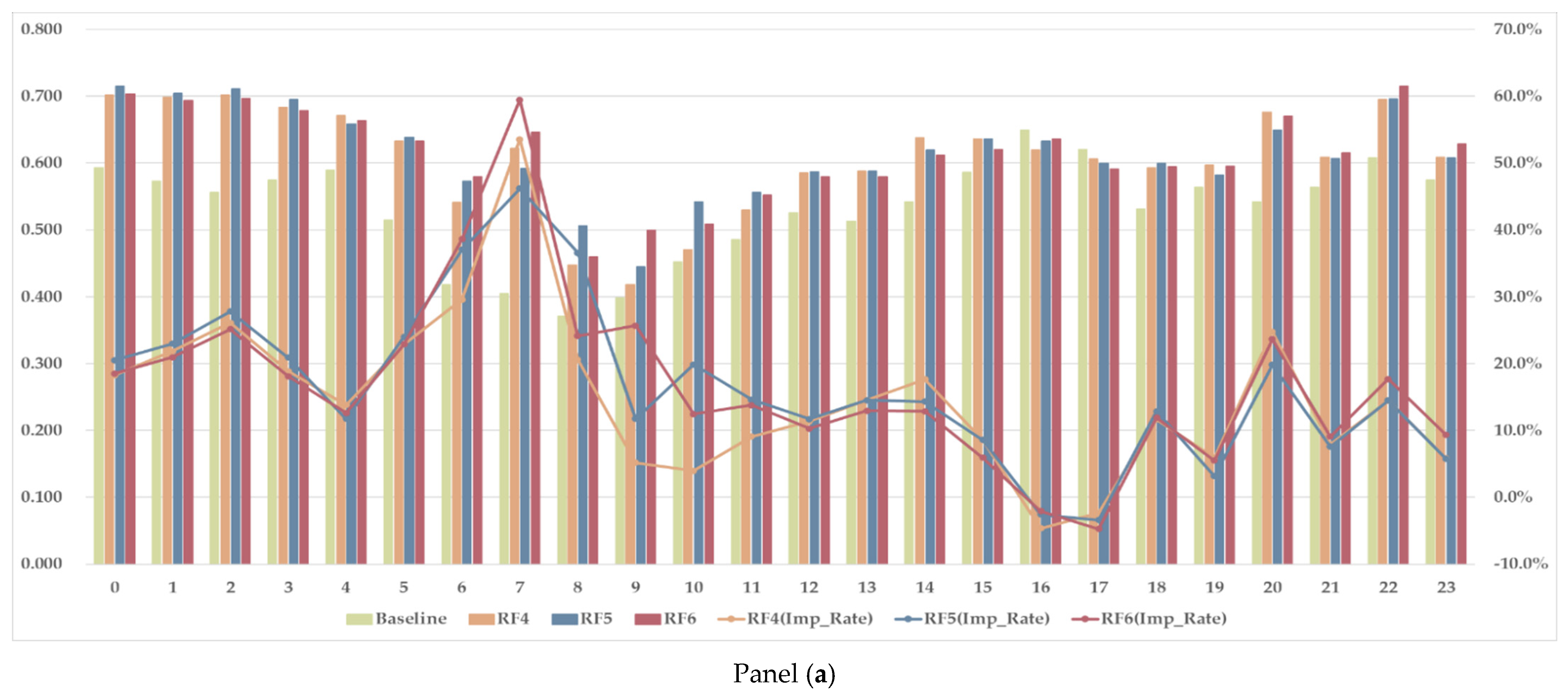
5.3. Hourly Trends in Forecasting Precision

Finally, we examine the hourly trends in forecasting performance. By analyzing the temporal patterns throughout the day, we aim to identify how forecasting difficulty varies at different times of the day, which is critical for improving operational decision-making.

Figure 10 presents the hourly ${Precision}_{shortage}$, with Panel (a) showing the results for the RF4–6 models and Panel (b) for the LGBM4–6 models. The bar charts display the precision values for each hour, while the line graphs indicate the improvement rate compared to the baseline. A key observation is that the baseline is outperformed at almost all hours, showing that models trained with statistical summaries and broader weather inputs provide meaningful predictive value. However, during 16:00–17:00, a slight reduction in precision is observed compared to the baseline, suggesting that the models face challenges in accurately classifying shortages during this period. This likely corresponds to the transition from late-afternoon to evening, when residential electricity demand rises as people return home from work. Unlike during the morning and midday hours, where solar power generation plays an important role, this period may involve a more complex imbalance mechanism, influenced by demand surges and shifting grid dispatch strategies.

The impact of multi-location weather data coverage is particularly notable from early-morning to noon, with models incorporating broader weather inputs achieving the most significant improvements compared to the baseline. This trend suggests that solar radiation in different regions contributes to enhanced predictability of shortages during the morning-to-midday hours. The alignment with the typical solar power generation profile across locations implies that the influence of renewable energy variability plays a critical role in system imbalances during this period.

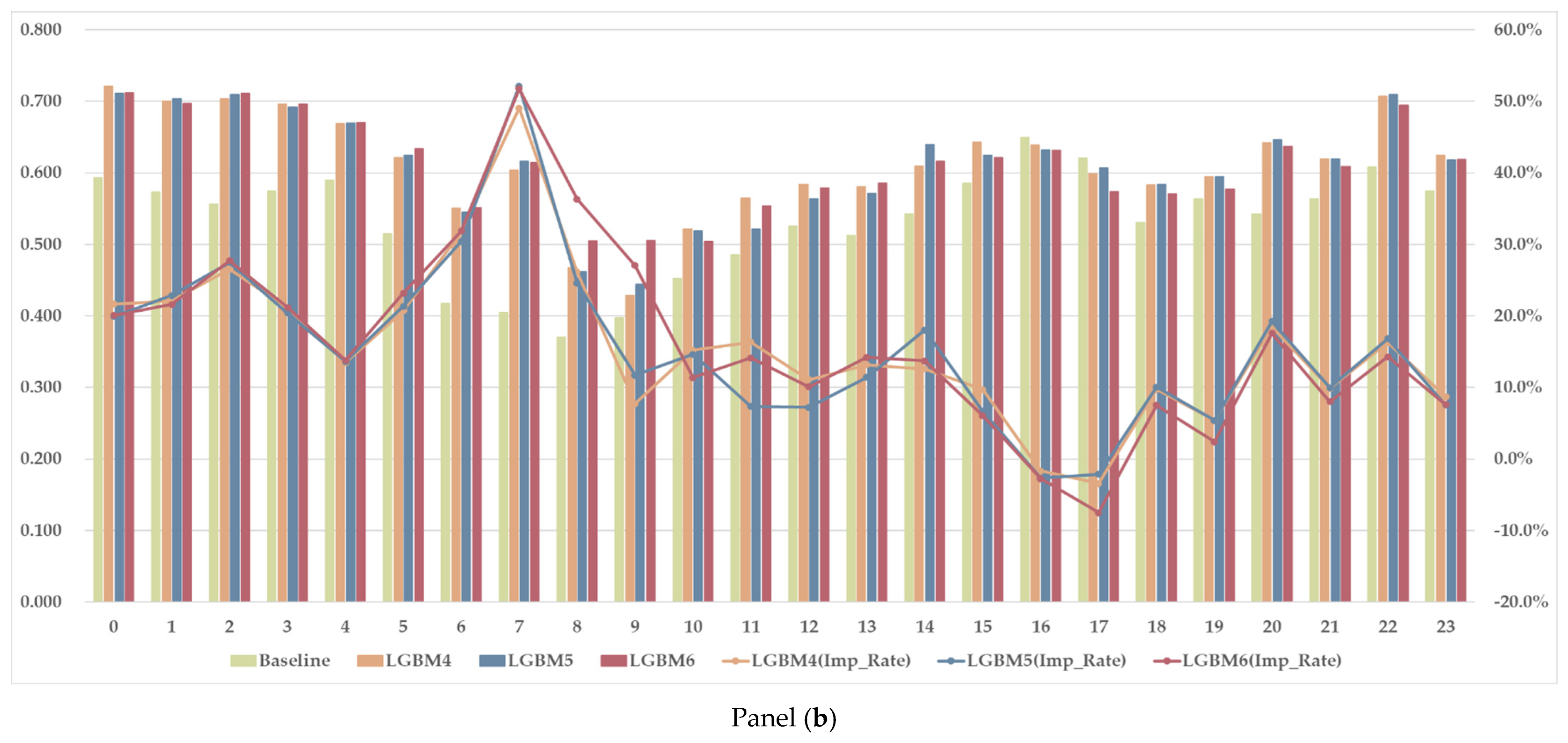
Figure 11 presents the hourly ${Precision}_{surplus}$, with Panel (a) showing the results for the LGBM1–3 models and Panel (b) for the LGBM4–6 models. The bar charts display the precision values for each hour, while the line graphs represent the improvement rate compared to the baseline. A key observation is that all hours outperform the baseline, confirming that the suggested models provide meaningful predictive value beyond historical trends.

Improvement rates vary across different time periods, influenced by patterns in feature engineering and the coverage of weather data. Models that incorporate broader weather data demonstrate improvements in predicting surplus events, highlighting the impact of spatially diverse weather features on forecast performance. The contribution of multi-location weather data is particularly evident from daytime to late-afternoon and from midnight to early-morning. This trend suggests that solar radiation and temperature variations across multiple locations strongly influence the predictability of surplus events, particularly during periods of high renewable energy generation and demand transitions. The improvements from daytime to late-afternoon indicate that solar power fluctuations across different regions significantly contribute to surplus events, aligning with the findings from the sensitivity analysis. Conversely, the improvements from midnight to morning suggest that regional temperature variations and late-night demand patterns may play a role in impacting supply–demand imbalances.

Overall, these findings further validate that spatially diverse weather features enhance surplus classification, particularly in periods affected by solar power generation. The consistent outperformance of all models compared to the baseline highlights the robustness of the proposed feature engineering and weather integration strategies. However, the results also suggest that surplus classification is impacted more directly by multi-location weather data than shortage classification, emphasizing the need to incorporate regional weather variability into surplus event prediction models.

6. Discussion

Balancing supply and demand in electricity markets is a constant and critical challenge, especially in systems with a high level of renewable energy penetration. System imbalance signals, which indicate whether the system is experiencing a shortage or surplus, are essential not only for TSOs to maintain grid stability, but also for market participants such as power producers and retailers. These signals directly influence participants’ trading strategies and risk management decisions, as they affect financial outcomes. In Japan, the shift to a single-pricing imbalance settlement system has further increased the importance of accurate forecasting, as it directly affects the costs or incentives faced by market participants, depending on their imbalance positions relative to the overall power system. This study has aimed to clarify the mechanisms driving imbalance signals and to evaluate the feasibility of using ML models for next-day forecasting, with the goal of improving operational decision-making.

To this end, we conducted a sensitivity analysis using LightGBM and SHAP to identify key drivers of system imbalances, and subsequently developed predictive models using LightGBM and RF. The findings and their implications for real-world market operations in Japan are discussed below:

• Sensitivity analysis using LightGBM and SHAP revealed that the mechanisms underlying imbalance signals are influenced by a complex set of features, including historical imbalance trends, weather conditions, market dynamics, and temporal patterns. Rather than being driven by a single dominant factor, imbalance signals emerge from the interplay of multiple variables, each of which contributes to fluctuations in supply and demand. Lagged imbalance demonstrated consistent predictive power, indicating that past imbalances tend to propagate over time due to structural and behavioral market patterns. Weather-related variables—particularly temperature, solar radiation, and the corresponding forecast errors—also played a crucial role, reflecting the dependency of electricity demand and renewable energy generation on weather conditions and their associated uncertainties.
• The impact of these features varied across both temporal and spatial dimensions. Solar radiation-related features, representing supply-side uncertainty from renewable energy generation, were most influential during the daytime, when solar power output fluctuated due to forecast errors. In contrast, temperature, which drives demand-side uncertainty, became more critical during evening and night-time periods, particularly in extreme seasons with surging heating and cooling demand. Calendar-related variables, such as weekends and public holidays, also exhibited greater importance in the evening, reflecting shifts in electricity consumption patterns. These temporal variations underscore the need for forecasting models that can account for the distinct drivers of imbalances at various times of the day.
• Spatial variations in feature importance further contributed to understanding the mechanisms behind system imbalances. The influence of temperature varied by location, with residential demand centers such as Yokohama (Kanagawa) showing stronger temperature sensitivity compared to commercial districts like Marunouchi in central Tokyo, where electricity demand tends to be more stable. Likewise, the impact of solar radiation differed across regions with high renewable penetration; for example, Tsukuba (Ibaraki) exhibited the strongest influence due to its significant solar power capacity. These spatial insights highlight the necessity of incorporating region-specific factors into imbalance signal forecasting, as different areas within the TEPCO region exhibit distinct supply and demand characteristics that affect overall system imbalances.
• Based on the findings from the sensitivity analysis, we also developed and evaluated next-day forecasting models designed to reflect real-world operational constraints. To ensure applicability under actual trading conditions, we carefully considered different feature engineering patterns. The forecasting models, which were built using RF and LightGBM, achieved strong overall accuracy and balanced precision when predicting both surplus and shortage classifications. Consequently, the developed tool offers practical value to market participants seeking to adjust their bidding and operational strategies ahead of the spot market.
• The forecasting results further emphasized that models leveraging broader spatial coverage of weather data consistently outperformed those using data from a single location, demonstrating the value of accounting for regional variations in renewable energy generation and temperature-driven demand. This effect was especially evident during daytime hours, when uncertainty relating to solar radiation played a dominant role in driving imbalances.
• Surplus events—often triggered by unexpected increases in renewable generation—were more accurately forecasted when multi-location weather data were included, as regional differences in solar power output became more significant. These findings highlight the critical role of spatially distributed weather data in capturing renewable generation dynamics, and underscore the need for forecasting frameworks that reflect weather variations across different locations in order to improve both predictive accuracy and operational decision-making.

7. Conclusions

This study has conducted a comprehensive analysis to improve the understanding of system imbalance signals and to develop practical prediction tools for the Japanese electricity market. Its contributions extend beyond methodological advancements, and include practical implications for market participants in real-world operations. By identifying the drivers of imbalance signals, the study provides actionable insights to support operational decision-making. The demonstrated ability to forecast imbalances with high precision enhances risk management practices, particularly in mitigating financial exposure to imbalance penalties. These findings are especially relevant in the context of Japan’s single-pricing mechanism, where alignment with system imbalance signals directly affects the financial outcomes of market participants.

From a broader perspective, the results highlight the vital role of accurate and timely weather-related forecasts in improving the efficiency and stability of Japan’s electricity market, as weather conditions—particularly temperature and solar radiation—significantly influence both electricity demand and renewable energy generation. However, the next-day grid forecasts for demand and renewable generation, which are published by TSOs at around 5 p.m. the day before, become available only after the spot and reserve markets have closed. To address this timing mismatch, it is crucial for TSOs to consider publishing longer-term system forecasts, thereby providing market participants with greater visibility into future conditions before spot market trading. Alternatively, policymakers and system operators should prioritize initiatives to activate Japan’s intraday market, which has experienced low trading volumes, despite its introduction in 2016. Encouraging greater participation in intraday trading would allow market participants to respond dynamically to emerging imbalances, leveraging updated forecasts and real-time system information. This would not only reduce reliance on TSOs for last-minute adjustments, but also foster a more flexible and adaptive electricity market.

We believe that the forecasting approach developed in this study could be extended beyond next-day predictions by incorporating updated weather-related information as it becomes available. Such an extension would also support more effective decision-making for intraday trading and real-time operations on the day of delivery.

We also recognize the importance of extending this research through a real-world case study, such as simulating bidding strategies or operational decisions based on the forecasted imbalance signals. Such a study would help to verify the financial outcomes of applying our predictive framework in practice. This would strengthen the link between predictive accuracy, operational behavior, and economic performance in real-world electricity markets. Furthermore, future research should also explore the adaptability of this approach in diverse market environments by assessing how model performance and the importance of key features change under varying conditions, such as different levels of renewable energy penetration and shifting demand patterns.