Optimizing Automatic Voltage Control Collaborative Responses in Chain-Structured Cascade Hydroelectric Power Plants Using Sensitivity Analysis

Abstract

Southwestern China has abundant hydropower networks, wherein neighboring cascade hydropower stations within the same river basin are typically connected to the power system in a chain-structured configuration. However, when such chain-structured cascade hydroelectric power plants (CC-HPPs) participate in automatic voltage control (AVC), problems such as reactive power interactions among stations and unreasonable voltage gradients frequently arise. To address these issues, this study proposes an optimized multi-station coordinated response control strategy based on sensitivity analysis and hierarchical AVC. Firstly, based on the topology of the chain-structured hydropower sending-end network, a reactive power–voltage sensitivity matrix is constructed. Subsequently, a regional-voltage-coordinated regulation model is developed using sensitivity analysis, followed by the establishment of a mathematical model, solution algorithm, and operational procedure for multi-station AVC-coordinated response optimization. Finally, case studies based on the actual operational data of a CC-HPP network validate the effectiveness of the proposed strategy, and simulation results demonstrate that the approach reduces the interstation reactive power pulling up to 97.76% and improves the voltage gradient rationality by 16.67%. These results substantially improve grid stability and operational efficiency while establishing a more adaptable voltage control framework for large-scale hydropower integration. Furthermore, they provide a practical foundation for future advancements in multi-scenario hydropower regulation, enhanced coordination strategies, and predictive control capabilities within clean energy systems.

1. Introduction

Hydropower, as a renewable and clean energy source, plays a key role in the functioning of power systems. Its efficient adjustment capability enables critical functions such as balancing supply and demand, regulating frequency, and controlling voltage [1,2,3]. As illustrated in Figure 1, multiple hydropower stations positioned at successive cascade levels within the same river basin are typically integrated into the power system in a chain-structured configuration, forming a cascade-connected hydropower plant (CC-HPP) sending-end network [4]. Within this network, upstream and downstream hydropower stations are hydraulically connected via natural water flow and electrically linked in sequence via transmission lines, collectively feeding power to a regional hub substation. Consequently, CC-HPPs demonstrate strong interdependence during hydropower production operations, large-scale system integration capacity, and significant power transfer effects [5]. These characteristics necessitate a shift from independent single-station control to coordinated multi-station regulation, thereby increasing operational complexity.

This complexity is further amplified during reactive power and voltage control. On the one hand, CC-HPPs, as power sources, typically require the voltage at the first station in the cascade to be approximately 5% higher than the rated voltage at the integration point [6,7,8]. Moreover, in some cases, the terminal station voltage may exceed the first station voltage by 15–20%, imposing greater demands on reactive power and voltage regulation. On the other hand, maintaining local reactive power balance, ensuring regional voltage stability, and achieving power flow equilibrium within CC-HPPs [9,10,11,12] not only require accounting for individual station characteristics but also demand coordination with global optimization objectives across the entire cascade. This interplay further increases the complexity of reactive power and voltage control.

Automatic voltage control (AVC), a reactive power and voltage regulation strategy widely implemented in contemporary power systems, is designed to ensure that voltage levels at substations and power sources remain within safe operational thresholds [13,14,15]. In CC-HPPs, the traditional AVC strategies primarily aim to stabilize the voltage at the regional hub substation by determining the voltage setpoints for each station and executing them with local AVC substations [16]. In situations where CC-HPPs are managed through centralized river basin control centers, voltage setpoints may be issued by the power grid dispatch center to the river basin control center, which then relays them to each station’s AVC substation [17]. The traditional AVC strategy in CC-HPPs has certain advantages and limitations. Its advantage lies in achieving real-time data acquisition and zoning control of the power grid through online partitioning and establishing mathematical models for each control area, thereby improving the accuracy and response speed of voltage control. However, this AVC strategy is primarily designed to optimize the global power grid and fails to comprehensively consider the strong interdependencies among CC-HPPs or their individual operational constraints. Consequently, challenges such as excessive interstation reactive power flows, abnormal voltage gradients, and difficulties in accurately tracking target voltage values frequently arise when CC-HPPs respond to AVC commands [18]. These issues prevent stations from complying with the regulatory requirements of China’s Grid-Connected Power Plant Operation Management Guidelines and Grid-Connected Power Plant Ancillary Services Management Guidelines [19], thereby impacting economic efficiency. They also intensify reactive power flow imbalances between stations, threatening overall grid stability [20]. These challenges underscore the limitations of traditional AVC strategies in satisfying the multi-station-coordinated operational demands of CC-HPPs, thereby necessitating the development of more refined reactive power and voltage control methods.

To address the complex coordinated regulation requirements of CC-HPPs, several advanced control approaches—such as model predictive control (MPC), distributed optimization, and deep learning—have demonstrated potential applicability. Among them, MPC offers advantages in handling dynamic optimization problems and is well suited for continuous control scenarios like reactive power regulation [21]. However, in multi-station, strongly coupled CC-HPP systems, the modeling of interdependencies is complex, and engineering deployment remains challenging. Distributed optimization is theoretically appropriate for multi-node systems like CC-HPPs [22]. Nevertheless, variations in the electrical locations of stations within the network can lead to divergent control objectives and priorities, thereby complicating unified coordinated modeling. Deep learning is effective in data-driven modeling, capable of capturing operational patterns and control behaviors [23]. However, since reactive power pulling is an infrequent and abnormal condition, data availability is limited. Furthermore, deep learning models often lack physical interpretability and are difficult to constrain within engineering parameters, posing challenges for direct application in power systems where safety and controllability are critical. Therefore, considering the current need for rapid and effective solutions to reactive power and voltage regulation anomalies in CC-HPPs, it is more practical to adopt a strategy that is mature in modeling, computationally efficient, and straightforward to deploy. Sensitivity analysis, a technique widely employed for reactive power optimization, voltage stability assessment, and dynamic response control in power systems [24,25,26,27,28], offers a means for this quantification. Wang et al. [29] proposed a resilience enhancement approach for interconnected electrical systems based on a global sensitivity analysis, improving system robustness under catastrophic conditions. BU Schyska et al. [30] proposed a sensitivity analysis framework for power system expansion models, assessing the impact of parameter changes on system planning. Further, Wang et al. [31] developed a refined power flow correction strategy based on a multimachine sensitivity analysis, enhancing real-time decision-making performance for power flow correction. In addition to the above factors, the traditional AVC approaches also rely on sensitivity-based control between power stations and the central hub [32]. However, to date, their implementation in CC-HPPs has not adequately considered interstation sensitivity, as the mutual influence among stations during reactive power regulation has been largely disregarded. Conducting a sensitivity analysis of CC-HPPs would enable researchers to quantify the impact of reactive power variations on voltage levels, providing a decision-making basis for improved reactive power and voltage regulation.

Reactive power–voltage sensitivity analysis can be leveraged to establish corresponding reactive power and voltage control strategies for precise AVC adjustments. However, certain intricate power grid structures continue to experience significant challenges in reactive power and voltage control when implementing AVC [33,34,35]. Wu et al. [36] proposed a reactive power distribution strategy based on AVC substations to alleviate reactive power output imbalances in large-scale new energy integration areas while ensuring voltage control. Wang et al. [37,38] introduced a voltage control strategy based on dynamic regulation and intelligent optimization to address the slow response times and limited control precision of traditional AVC methods for ultra-high-voltage networks. Shi et al. [39,40,41] optimized interplant coordination mechanisms by implementing plant-to-plant coordination techniques, mitigating reactive power output imbalances among strongly coupled power plants managed by closed-loop AVC. These studies indicate that effective reactive power and voltage control strategies must be tailored to specific grid structures based on their distinctive characteristics. While CC-HPPs differ in structural and operational aspects from other power grid networks, they share common challenges, such as unbalanced reactive power distribution, inadequate response precision, and limited adaptability in control. Drawing inspiration from solutions designed for other specialized power grid structures, this study adopts a coordinated optimization approach and adapts it to the operational characteristics of CC-HPPs to establish an AVC collaborative response optimization strategy.

To address the aforementioned challenges, this study focuses on chain-structured cascade hydroelectric power plants and aims to increase the effectiveness of AVC coordination through sensitivity-based optimization. The specific research objectives are as follows:

(1)

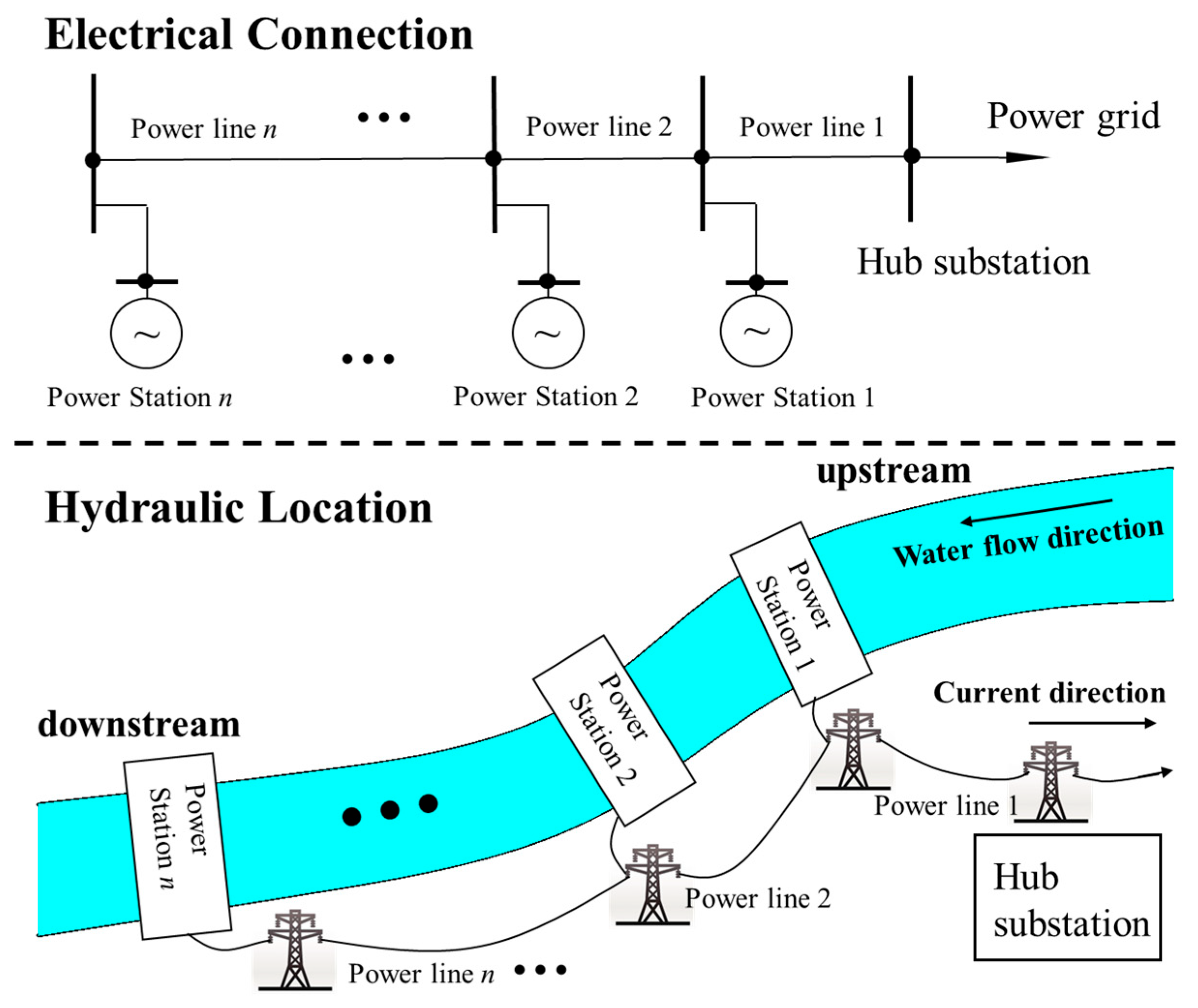
Analyze the mechanism of reactive power pulling induced by AVCs in CC-HPP networks.

(2)

Construct a reactive power–voltage coupling model on the basis of sensitivity analysis.

(3)

Propose a coordinated optimization strategy, and develop a regional voltage control system.

(4)

Conduct simulations and field-data-based validations to evaluate the effectiveness of the proposed strategy.

In summary, existing AVC strategies in cascade chain-structured hydropower networks have not adequately accounted for the strong electrical coupling between stations and their respective operational constraints, often resulting in unbalanced regional reactive power distribution and low voltage regulation efficiency. To address these challenges, this study proposes a sensitivity analysis-based coordinated response optimization strategy, derived from the structural characteristics of chain-structured hydropower systems. The strategy is designed to achieve refined voltage coordination among multiple stations, enhance regional power factor performance, and further improve the operational stability and overall control efficiency between cascade hydropower systems and the power grid.

2. Problem Statements

Figure 2 illustrates the problem under investigation, using the reactive power and voltage abnormalities observed when three hydropower stations in a CC-HPP network participate in the AVC as an example.

In Figure 2a, Station A consistently absorbs reactive power during operation, whereas Station B continuously generates reactive power. The shaded region in the figure represents the amount of reactive power generated by Station B that is absorbed internally within the CC-HPP network, thereby reducing the actual reactive power injected into the power grid. Meanwhile, in Figure 2b, substantial deviations are apparent between the operating voltages of both stations and their AVC-set references. The operating voltage of Station A often exceeds the AVC deadband, triggering counter-regulation actions in the AVC system. In contrast, the operating voltage of Station B consistently remains above the AVC deadband, preventing it from adjusting to the reference value.

The phenomenon in which reactive power generated by certain stations within the CC-HPP network is absorbed by adjacent stations without contributing to voltage stability—while also causing frequent high-voltage busbar voltage fluctuations and unreasonable voltage gradients—is defined as reactive power pulling in this study. Such pulling occurs when some stations generate substantial reactive power, while others absorb excessive amounts of this power, resulting in inefficient voltage regulation. Reactive power pulling induces frequent voltage deviations and heightens the risk of over- or under-excitation in generators at affected stations. This results in reduced water use efficiency and diminished generation performance, thereby compromising the safe, stable, and economical operation of individual stations and decreasing overall system productivity. In severe cases, inadequate voltage regulation caused by reactive power pulling can lead to power factor penalties and inefficient dispatch. For instance, if a 600 MW-class station operates under over-excited conditions that reduce its active power output by merely 3%, the resulting annual energy loss may exceed 12 GWh—equivalent to a direct economic loss of over CNY 6 million, based on a typical hydropower tariff of 0.5 CNY/kWh. These impacts underscore the urgent need to enhance reactive power coordination in CC-HPP networks.

When reactive power pulling occurs, CC-HPPs not only fail to accurately follow AVC voltage instructions and adhere to regulatory requirements but also experience unnecessary interstation reactive power losses during voltage tracking. In a more secure and economically efficient operational design, one station would supply the reactive power required for grid integration while other stations maintain low reactive power outputs. To determine the underlying causes of reactive power pulling in CC-HPP networks managed by closed-loop AVC, reactive power and voltage variations in the system’s power flow conditions must be analyzed.

Based on the typical CC-HPPs structure illustrated in Figure 1, an equivalent circuit model comprising n stations is developed, as depicted in Figure 3.

To simplify the analysis, each station is modeled as a generator–transformer unit. The equivalent circuit comprises 2n + 1 nodes, where n nodes (Nodes 1 to n) correspond to the high-voltage bus nodes of the stations. These nodes lack voltage regulation capability, implying that their power inflow equals their power outflow. Consequently, they are modeled as PQ nodes with zero active (P) and reactive (Q) power. An additional set of n nodes (Nodes n + 1 to 2n) corresponds to the generator terminal nodes of the stations. Given that generators can regulate voltage, these nodes are typically treated as PV nodes in power system analysis. One additional node (Node 0) represents the high-voltage bus node of the hub substation, which is directly connected to the external infinite system and functions as the slack (balance) node.

A change in the power flow through the high-voltage bus node of a station induces variations in the high-voltage bus voltage. Considering station i in Figure 3 as an example, if the power flowing from station i + 1 into station i is P_i + jQ_i, the high-voltage bus voltage at station i is U_i. When the incoming power changes to P_i′ + jQ_i′, the high-voltage bus voltage at station i changes to U_i′. The voltage variation ΔU_i at station i in this scenario can be approximately expressed as [42]

$$\Delta U_i=U_i^{\prime }-U_i={\displaystyle \frac{(P_i^{\prime }-P_i)R_i+(Q_i^{\prime }-Q_i)X_i}{U_{i+1}}}$$

(1)

where P_i and Q_i denote the initial active and reactive power flowing from station i + 1 to station i, respectively; P_i′ and Q_i′ represent the active and reactive power after the change; R_i and X_i signify the resistance and reactance of the transmission line between station i + 1 and station i, respectively; and U_i+1 denotes the high-voltage bus voltage at station i + 1, which corresponds to the sending-end voltage of the transmission line.

In high-voltage transmission systems, the line reactance is substantially greater than the resistance (i.e., X_i ≫ R_i), and the voltage is far more sensitive to variations in reactive power than in active power [43]. To emphasize this dominant relationship and simplify the analytical model, the resistance term in Equation (1) is omitted in this study. This results in a simplified expression that considers only the effect of reactance, as presented in Equation (2). This approximation is commonly employed in high-voltage power system analysis, as it has a negligible impact on the accuracy of reactive power regulation and voltage sensitivity assessments, while substantially improving computational efficiency and model clarity.

$$\Delta U_i={\displaystyle \frac{(Q_i^{\prime }-Q_i)X_i}{U_{i+1}}}$$

(2)

Because CC-HPPs are integrated into the power system as a sending-end network, the reactive power generated by each station under AVC regulation inevitably traverses the high-voltage bus of other stations before being delivered to the grid. When the traditional AVC strategy fails to account for the impact of this transferred reactive power, it is effectively treated as Q_i′, creating a deviation ΔU_i between the actual and set voltages at the station. If ΔU_i exceeds the AVC deadband, the AVC substation at the station reduces the reactive power output of its generator to track the voltage setpoint. This action reduces the reactive power flowing through the bus of the neighboring station, leading to a voltage drop. In response, the AVC substation of the neighboring station boosts the generation of reactive power to restore the voltage, which, in turn, raises the bus voltage of the original station and reduces the reactive power output at this location. This process creates a self-reinforcing cycle in which some stations generate excessive reactive power, while others absorb excessive amounts of it. Consequently, voltage fluctuations frequently occur at each station, causing the voltage to deviate from AVC voltage setpoints and ultimately leading to an unreasonable regional voltage gradient across the CC-HPP network.

To address this issue, this study proposes a reactive power–voltage sensitivity analysis approach to quantify the effects of reactive power transfer on station voltages. Based on the results, an optimal control strategy and corresponding reactive power and voltage operational indices are established to overcome AVC-related challenges in CC-HPPs.

3. Sensitivity Analysis

Sensitivity analysis, as a key method in reactive power and voltage control research for power systems [40], quantifies the influence of variations in system variables on output parameters. By evaluating the sensitivity of voltage to reactive power, the high-voltage busbar voltage can be regulated by adjusting the reactive power output of generators. This provides a theoretical basis for optimizing regional reactive power and voltage control strategies.

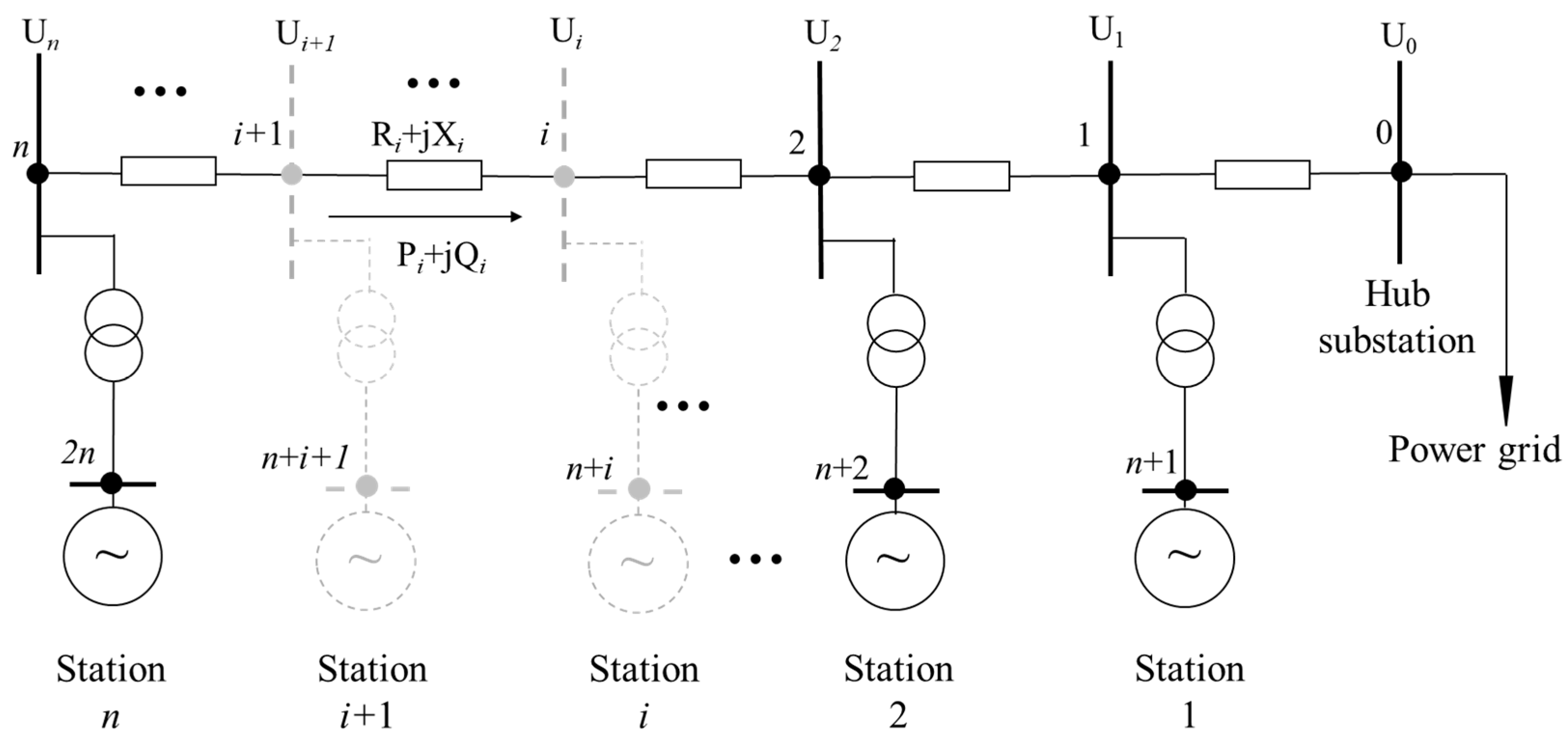
3.1. Sensitivity Modeling

Reactive power–voltage sensitivity calculations are primarily based on power flow analysis in power systems [44]. Among the available methods for these calculations, the Newton–Raphson method is widely adopted due to its rapid convergence and efficiency in solving nonlinear power flow equations. For a CC-HPP network comprising n power stations and 2n + 1 nodes, the nodal power equations in polar coordinates are expressed as follows:

$$\left\{\begin{array}{c}{P}_a=V_a{\displaystyle \sum _{a\in b}^{2n+1}}{V}_b(G_{ab}\mathit{cos}{\theta }_{ab}+B_{ab}\mathit{sin}{\theta }_{ab})\\ Q_a=V_b{\displaystyle \sum _{a\in b}^{2n+1}}{V}_b(G_{ab}\mathit{sin}{\theta }_{ab}-B_{ab}\mathit{cos}{\theta }_{ab})\end{array}\right.$$

(3)

where a and b denote any two interconnected nodes in the 2n + 1 node equivalent circuit of the CC-HPP network, with a ∈ b indicating connectivity between nodes a and b. Further, the parameters P_a and Q_a represent the active and reactive power at node a, respectively; V_a denotes the voltage magnitude at node a; θ_ab signifies the voltage phase angle difference between nodes a and b; and G_ab and B_ab represent the real and imaginary components of the admittance matrix element Y_ab, respectively.

(1) By addressing the system’s power mismatches, the following power flow equations are obtained:

$$\left\{\begin{array}{c}\Delta P_a=P_{Ga}-P_{La}-V_a{\displaystyle \sum _{a\in b}^{2n+1}}{V}_b(G_{ab}\mathit{cos}{\theta }_{ab}+B_{ab}\mathit{sin}{\theta }_{ab})\\ \Delta Q_a=Q_{Ga}-Q_{La}-V_b{\displaystyle \sum _{a\in b}^{2n+1}}{V}_b(G_{ab}\mathit{sin}{\theta }_{ab}-B_{ab}\mathit{cos}{\theta }_{ab})\end{array}\right.$$

(4)

where ΔP_a and ΔQ_a denote the active and reactive power mismatches at node a, respectively; P_Ga and Q_Ga represent the active and reactive power injected at node a; and P_La and Q_La signify the active and reactive power consumed at node a, respectively.

(2) A typical CC-HPP network equivalent circuit comprises 2n + 1 nodes. Among these, Nodes 1 to n are classified as PQ nodes, contributing 2n equations. Further, Nodes n + 1 to 2n fall under PV nodes, contributing n equations. By expanding the nonlinear power flow expressions in Equation (4) using Taylor series and disregarding higher-order terms, the following linear system of 3n equations is derived:

$$\left[\begin{array}{c}\Delta P_1\\ \Delta Q_1\\ ⋮\\ \Delta P_n\\ \Delta Q_n\\ \Delta P_{n+1}\\ ⋮\\ \Delta P_{2n}\end{array}\right]=\left[\begin{array}{cccccccc}{H}_{11}& N_{11}& \cdots & H_{1n}& N_{1n}& H_{1,n+1}& \cdots & H_{\mathrm{1,2}n}\\ M_{11}& L_{11}& \cdots & M_{1n}& L_{1n}& M_{1,n+1}& \cdots & M_{\mathrm{1,2}n}\\ ⋮& ⋮& ⋮& ⋮& ⋮& ⋮& ⋮& ⋮\\ H_{n1}& N_{n1}& \cdots & H_{nn}& N_{nn}& H_{n,n+1}& \cdots & H_{n,2n}\\ M_{n1}& L_{n1}& \cdots & M_{nn}& L_{nn}& M_{n,n+1}& \cdots & M_{n,2n}\\ H_{n+\mathrm{1,1}}& N_{n+\mathrm{1,1}}& \cdots & H_{n+1,n}& N_{n+1,n}& H_{n+1,n+1}& \cdots & H_{n+\mathrm{1,2}n}\\ ⋮& ⋮& ⋮& ⋮& ⋮& ⋮& ⋮& ⋮\\ H_{2n,1}& N_{2n,1}& \cdots & H_{2n,n}& N_{2n,n}& H_{2n,n+1}& \cdots & H_{2n,2n}\end{array}\right]\left[\begin{array}{c}\Delta {\theta }_1\\ \Delta V_1\\ ⋮\\ \Delta {\theta }_n\\ \Delta V_n\\ \Delta {\theta }_{n+1}\\ ⋮\\ \Delta {\theta }_{2n}\end{array}\right]$$

(5)

When expressed in block matrix form, this system can be represented as

$$\left[\begin{array}{c}\Delta P\\ \Delta Q\end{array}\right]=\left[\begin{array}{cc}H& N\\ M& L\end{array}\right]\left[\begin{array}{c}\Delta \theta \\ \Delta V\end{array}\right]$$

(6)

where ΔV and Δθ represent variations in voltage magnitude and phase angle, respectively; N and H denote the partial derivative matrices of active power with respect to the voltage magnitude and phase angle, respectively; and L and M signify the partial derivative matrices of reactive power with respect to the voltage magnitude and phase angle, respectively.

(3) Given the relatively weak coupling between active power and voltage magnitude, the influence of active power on nodal voltage is often disregarded during analysis. This is achieved by setting ΔP = 0. By transforming the linearized power flow equations, the sensitivity matrix C of the system can be obtained as follows:

$$C={\displaystyle \frac{\Delta V}{\Delta Q}}={\left[L-M{H}^{-1}N\right]}^{-1}$$

(7)

Thus, analyzing the reactive power–voltage sensitivity in CC-HPPs necessitates the construction of a power flow model based on the network’s topology, derivation of the sensitivity matrix, and estimation of the impact of reactive power variations on node voltages.

3.2. Reactive Power–Voltage Sensitivity Analysis of CC-HPPs

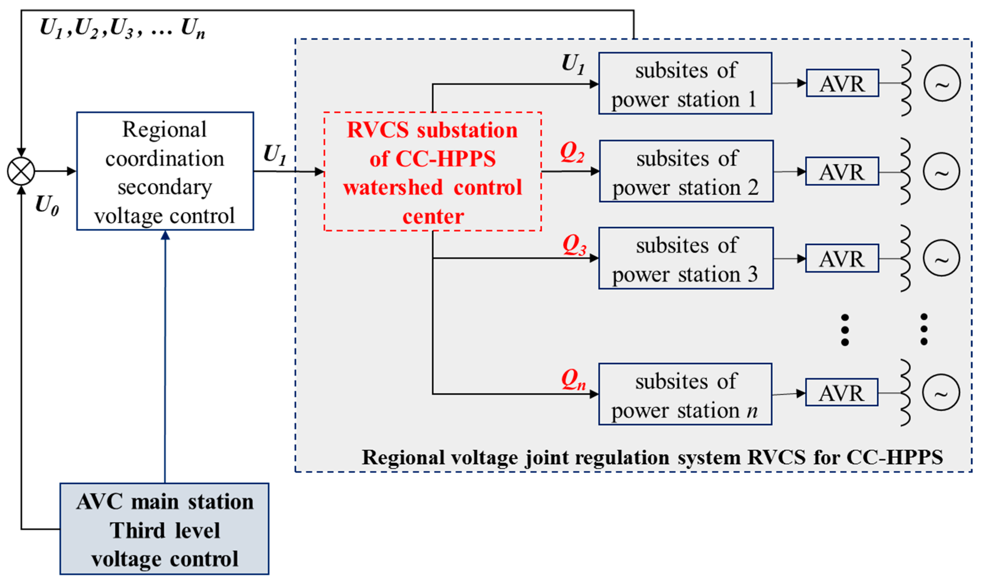
Traditional sensitivity calculations only account for PQ nodes. However, to examine the impact of reactive power output variations at different power stations on busbar voltages, a sensitivity matrix incorporating PV nodes must be constructed. As illustrated in Figure 4, the process for deriving the full sensitivity matrix involves repeated power flow calculations [45].

Because the power flow model incorporates equivalent transformers and generators, system parameters vary with operating conditions. Hence, the actual system parameters must first be incorporated into the power flow equations to construct the nodal admittance matrix for the initial power flow calculation under current operating conditions. Next, based on the power flow results, PV nodes must be converted into PQ nodes, enabling the development of a new power flow equation set that includes PV nodes. Through repeated power flow calculations, the full Jacobian matrix—excluding the slack node—should be derived, ultimately enabling the formulation of a sensitivity matrix incorporating PV nodes.

After modifying the PV nodes using this method, the power flow equations incorporating PV nodes can be expressed as follows:

$$\left[\begin{array}{c}\Delta P_1\\ \Delta Q_1\\ ⋮\\ \Delta P_{2n}\\ \Delta Q_{2n}\end{array}\right]=\left[\begin{array}{ccccc}{H}_{11}& N_{11}& \cdots & H_{1n}& N_{1n}\\ M_{11}& L_{11}& \cdots & M_{1n}& L_{1n}\\ ⋮& ⋮& ⋮& ⋮& ⋮\\ H_{2n,1}& N_{2n,1}& \cdots & H_{2n,2n}& N_{2n,2n}\\ M_{2n,1}& L_{2n,1}& \cdots & M_{2n,2n}& L_{2n,2n}\end{array}\right]\left[\begin{array}{c}\Delta {\theta }_1\\ \Delta V_1\\ ⋮\\ \Delta {\theta }_{2n}\\ \Delta V_{2n}\end{array}\right]$$

(8)

By setting ΔP = 0, the linearized power flow equations can be transformed to obtain the reactive power–voltage sensitivity matrix C, as expressed in Equation (9). This matrix incorporates the sensitivity of Nodes 1 to 2n.

$$C=\left[\begin{array}{cccccc}{C}_{11}& \cdots & C_{1,n}& C_{1,n+1}& \cdots & C_{\mathrm{1,2}n}\\ ⋮& \ddots & ⋮& ⋮& \ddots & ⋮\\ C_{n,1}& \cdots & C_{n,n}& C_{n,n+1}& \cdots & C_{n,2n}\\ C_{n+\mathrm{1,1}}& \cdots & C_{n+1,n}& C_{n+1,n+1}& \cdots & C_{n+\mathrm{1,2}n}\\ ⋮& \ddots & ⋮& ⋮& \ddots & ⋮\\ C_{2n,1}& \cdots & C_{2n,n}& C_{2n,n+1}& \cdots & C_{2n,2n}\end{array}\right]=\left[\begin{array}{cc}{C}_1& C_2\\ C_3& C_4\end{array}\right]$$

(9)

where C₁₁ denotes the voltage variation at Node 1 when the reactive power at this node changes by one unit, $C_{1,n}$ represents the voltage variation at Node n when the reactive power at Node 1 changes by one unit, and so forth. The submatrices C₁, C₂, C₃, and C₄ are n-dimensional.

Nodes 1 to n represent high-voltage bus PQ nodes with zero power, while Nodes n + 1 to 2n denote generator bus PV nodes. Therefore, in the reactive power–voltage sensitivity matrix C of CC-HPPs, only rows (n + 1) to 2n (corresponding to submatrices C₃ and C₄) have actual physical significance. When all power stations within the CC-HPP network participate in reactive power regulation, the resulting voltage variation ΔU at the high-voltage bus of any station x in the network can be expressed as follows:

$$\Delta U={\displaystyle \sum _{i=1}^n}{C}_{n+i,x}\Delta Q_{n+i}$$

(10)

where i represents the station index in the CC-HPP network, $\Delta Q_{n+i}$ denotes the reactive power adjustment at the generator bus node of station i, and $C_{n+i,x}$ signifies the reactive power–voltage sensitivity of the generator bus node of station i relative to the high-voltage bus node of station x.

Given that system parameters vary with operating conditions, it is necessary to incorporate real-time parameters into the power flow model before conducting sensitivity analysis for reactive voltage regulation, in order to construct the Jacobian matrix corresponding to the current time step and ensure accurate sensitivity calculations. Specifically, if the current regulation time is t, then the sensitivity matrix C^t should be computed based on the system parameters at time t; in the subsequent cycle, the parameters should be updated to those at time t + 1, resulting in a new matrix C^t+1. Accordingly, the sensitivity matrix evolves dynamically with each regulation cycle, following a time sequence of “C^t−1 → C^t → C^t+1”. Under this framework, Equation (10) at time t can be further represented as Equation (11).

$$\Delta U^t={\displaystyle \sum _{i=1}^n}{C}_{n+i,x}^t{\Delta Q}_{n+i}^t$$

(11)

where t denotes the t-th cycle of reactive power regulation. In the following context, t refers to the current regulation cycle, t + 1 indicates the next cycle, and t − 1 indicates the previous cycle.

In summary, the reactive power–voltage sensitivity matrix, derived from the power flow model of the CC-HPP network, serves to quantify how changes in reactive power output at individual stations affect the voltage levels at high-voltage buses within the network. Since the matrix is updated in real time during each control cycle, it accurately reflects the system’s changing operating conditions and enables responsive regulation. By leveraging this time-resolved analysis, sensitivity indices can be applied as core control variables to fine-tune generator reactive power outputs, allowing for precise and adaptive voltage control across high-voltage nodes. This real-time sensitivity-based approach establishes a strong analytical framework for advancing regional reactive power and voltage regulation strategies.

4. Control Strategy

To realize coordinated optimization control for CC-HPPs, this study proposes a collaborative response mechanism and regulation process that integrates internal reactive power optimization with a reactive power response at the grid integration point. Based on the reactive power–voltage sensitivity matrix, an optimization model and a set of evaluation indices were established to ensure the optimal distribution of reactive power within the network, thereby enhancing security, economic efficiency, and operational stability.

4.1. Control Model

As illustrated in Figure 5, this study establishes a regional voltage control system (RVCS) based on sensitivity analysis to implement an AVC strategy integrated with a provincial dispatch-centralized control-power station framework for CC-HPPs. The RVCS was deployed at the river basin control center to coordinate AVC operations with the power grid.

In this control model, the grid AVC master station optimized power flow by calculating the high-voltage bus voltage U₀ at the hub substation within the CC-HPP network. This calculated voltage was then relayed to the regional coordination secondary voltage controller. To maintain U₀, the secondary voltage controller converted the reactive power demand of the CC-HPP network into a corresponding high-voltage bus voltage setpoint U₁ at the grid connection point. This was accomplished using reactive power–voltage sensitivity analysis. The established setpoint U₁ was then dispatched to the RVCS substation at the centralized hydropower control center. This substation, tasked with maintaining U₁ and optimizing the reactive power output within the network, formulated an interstation-coordinated reactive power optimization model based on sensitivity analysis. It determines the reactive power outputs Q₂ to Q_n, which were subsequently dispatched to the AVC substations of individual stations for implementation. Through this strategy, the control model of CC-HPPs transitions from independent station responses to grid AVC to a coordinated response mechanism wherein the RVCS responds to the grid while individual stations operate under RVCS constraints. This provincial dispatch-centralized control-power station framework ensures that the CC-HPP network meets grid reactive power demands while enhancing internal power factor performance.

From an engineering perspective, the regional voltage control system (RVCS) was installed at the centralized control center of the river basin, where it integrates seamlessly with the existing SCADA and AVC infrastructure. It gathers real-time operational data from all stations via the wide-area communication network and runs optimization algorithms based on the current system conditions. The resulting optimized reactive power setpoints were then transmitted to the local AVC systems at each station for execution. This implementation makes full use of the existing communication and automation infrastructure, requiring no additional hardware, thereby ensuring system compatibility, low deployment cost, and fast scalability across CC-HPP networks. As depicted in Figure 6, the control cycle of the RVCS operates on the same 5 min time scale as the AVC model [16]. Within each AVC cycle, the RVCS performs optimization calculations and implements adjustments during a designated time window once the assessment period commences.

The control process of the RVCS comprises three stages within each 5 min AVC cycle:

Stage I (0–2 min): The power station at the grid connection point responds to the AVC voltage command and makes the necessary adjustments.

Stage II (2–3 min): At the 2 min mark, the grid connection point power station begins to maintain voltage and accepts grid AVC assessment. Moreover, the RVCS collects the operating parameters of this cycle and calculates the optimized regulation of other power stations in the area.

Stage III (3–5 min): Once the assessment period ends, the remaining stations in the network receive and implement the RVCS optimization adjustments.

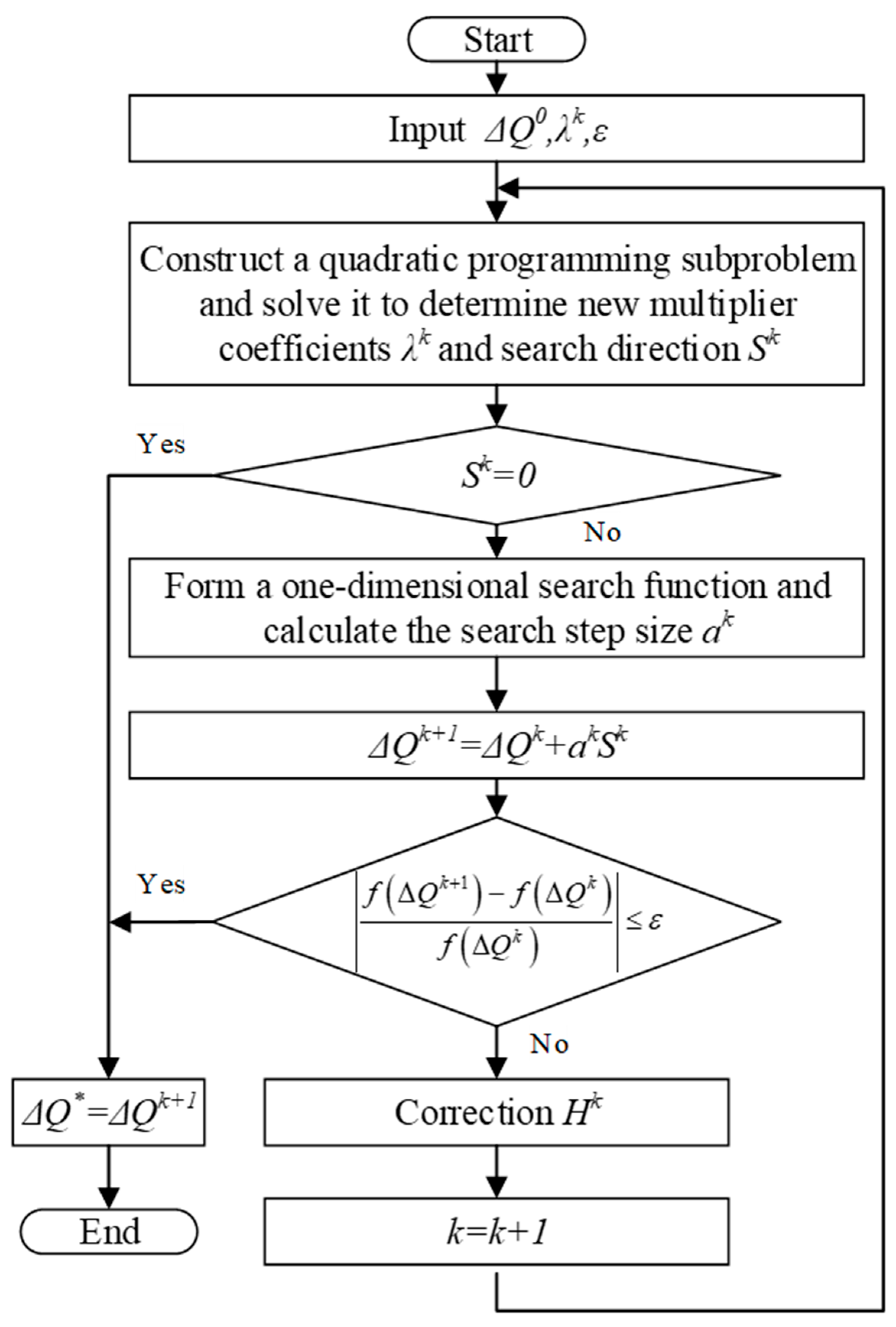
4.2. Mathematical Modeling

To implement collaborative AVC response control in CC-HPPs, the RVCS must solve an optimization problem that accounts for both interstation coordination and operational constraints.

4.2.1. Objective Function

In the AVC-coordinated response control mode for CC-HPPs, only the station at the grid connection point directly responds to AVC commands to satisfy hub voltage requirements, ensuring grid security and stability. Meanwhile, the remaining stations within the network aim to minimize the total reactive power output. Thus, by defining the reactive power adjustment ΔQ_g of each station as the control parameter, the objective function was formulated to minimize the total reactive power output of the remaining stations within the network:

$$\underset{\Delta Q_{n+i}}{min}\left\{{\displaystyle \sum _{i=2}^n}{W}_i(Q_{n+i}^t+\Delta Q_{n+i}^t{)}^2\right\}$$

(12)

where i represents the index of the n − 1 stations in the CC-HPP network requiring optimization, sequentially numbered 2, 3, …, n; $\Delta Q_{n+i}^t$ denotes the reactive power adjustment of station i during the current regulation cycle t; $Q_{n+i}^t$ represents the current reactive power output of station i during the current regulation cycle t; and W denotes the weighting coefficient.

When the reactive power adjustment $\Delta Q_{n+i}^t$ is set as the negative of the current reactive power output $Q_{n+i}^t$, the total reactive power output within the network is minimized. However, the cumulative effect of substantial reactive power adjustments across multiple stations may induce extensive voltage fluctuations at the grid connection point bus. Therefore, constraints must be established based on reactive power–voltage sensitivity analysis to quantify the impact of each station’s reactive power adjustment on the grid connection point voltage. By accounting for these constraints, the optimal reactive power operating state of each station can be identified, ensuring effective AVC while maintaining grid security and stability.

4.2.2. Constraints

(1)

Constraint on Voltage Variation at the Centralized Grid Connection Point of the CC-HPP Network

Regional reactive power optimization must be performed in compliance with grid AVC regulations. Therefore, accounting for the impact of regional reactive power optimization adjustments on the bus voltage at the grid connection point is essential. By restricting voltage variations within the AVC deadband, the adjustment ensures that the grid AVC effectively regulates the voltage at the grid connection point, ensuring system stability.

$$\left|{\displaystyle \sum _{i=2}^n}{C}_{n+i,1}^t\Delta Q_{n+i}^t\right|\le U_1^{dz}$$

(13)

where $C_{n+i,1}^t$ represents the reactive power–voltage sensitivity of the generator bus at station i with respect to the high-voltage bus at the grid connection point (node n + 1) during the current regulation cycle t, and U₁^dz denotes the AVC deadband voltage limit set by the power grid.

(2)

Constraint on the Voltage Gradient Difference Across High-Voltage Bus Nodes in the CC-HPP Network

In the CC-HPP network, high-voltage bus voltages must exhibit a decreasing gradient from Node n to Node 1. At the beginning of Stage II in regulation cycle t, if the voltage gradient between two neighboring stations i and i − 1 satisfies the condition U_i^t > U_i−1^t, the constraint to be implemented is as expressed in Equation (14). Otherwise, the constraint follows Equation (15).

$$\Delta U_{i,i-1}^{t+1}>0$$

(14)

$$\Delta U_{i,i-1}^{t+1}>\Delta U_{i,i-1}^t$$

(15)

$$\Delta U_{i,i-1}^{t+1}=\left(C_{n+i,i}^t\Delta Q_{n+i}^t+U_i^t\right)-\left(C_{n+i-1,i-1}^t\Delta Q_{n+i-1}^t+U_{i-1}^t\right)$$

(16)

$$\Delta U_{i,i-1}^t=U_i^t-U_{i-1}^t$$

(17)

where ΔU_i,i−1^t denotes the voltage gradient between two neighboring stations i and i − 1 at the 2 min of regulation cycle t; ΔU_i,i−1^t+1 denotes the voltage gradient between two neighboring stations i and i − 1 at minute 0 of the next regulation cycle t + 1; $C_{n+i,i}^t$ signifies the reactive power–voltage sensitivity of the generator bus node n + i at station i relative to its high-voltage bus node i; and U_i^t represents the current voltage at the high-voltage bus node i of station i.

(3)

Constraint on the Single-Station Adjustment Step Size

This constraint was used to limit the speed and amplitude of voltage changes in the busbars of various power stations within the region, ensuring the stability of system operation and the controllability of the regulation process.

$$\left|C_{n+i,i}^t\Delta Q_{n+i}^t\right|\le \Delta U_i^{max}$$

(18)

where ΔU_i^max denotes the maximum voltage adjustment step size for the high-voltage bus node (n + 1) of station i.

(4)

Constraint on Single-Station Voltage Limits

The bus voltage of the power station must be maintained within the specified range during operation to ensure the safe functioning of system equipment and the quality of grid voltage.

$$U_i^{min}\le {U_i^t+C}_{n+i,i}^t\Delta Q_{n+i}^t\le U_i^{max}$$

(19)

where $U_i^{max}$ and $U_i^{min}$ denote the upper and lower operating voltage limits, respectively, for high-voltage bus node i within an individual station.

(5)

Constraint on the Single-Station Reactive Power Output Limits

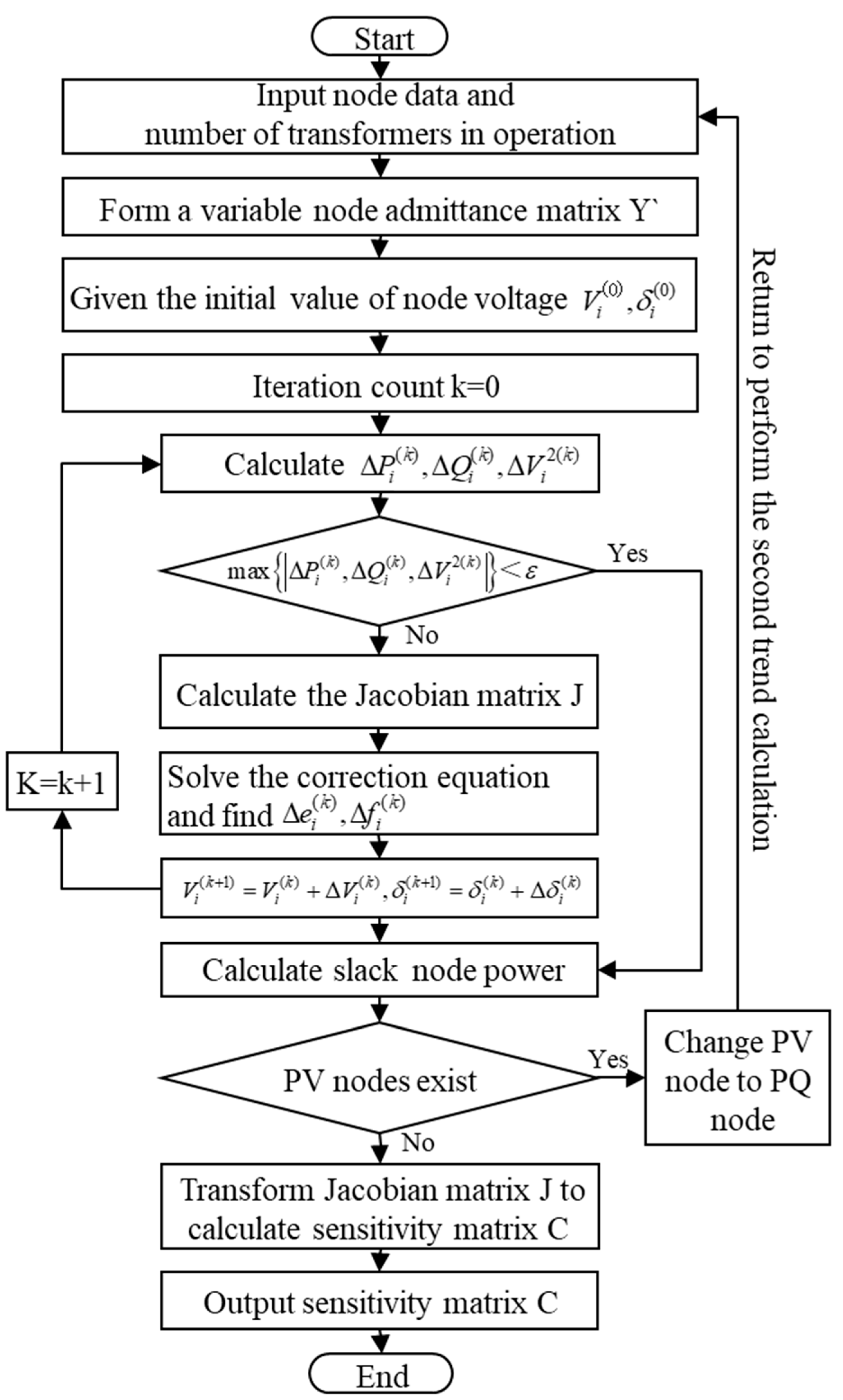
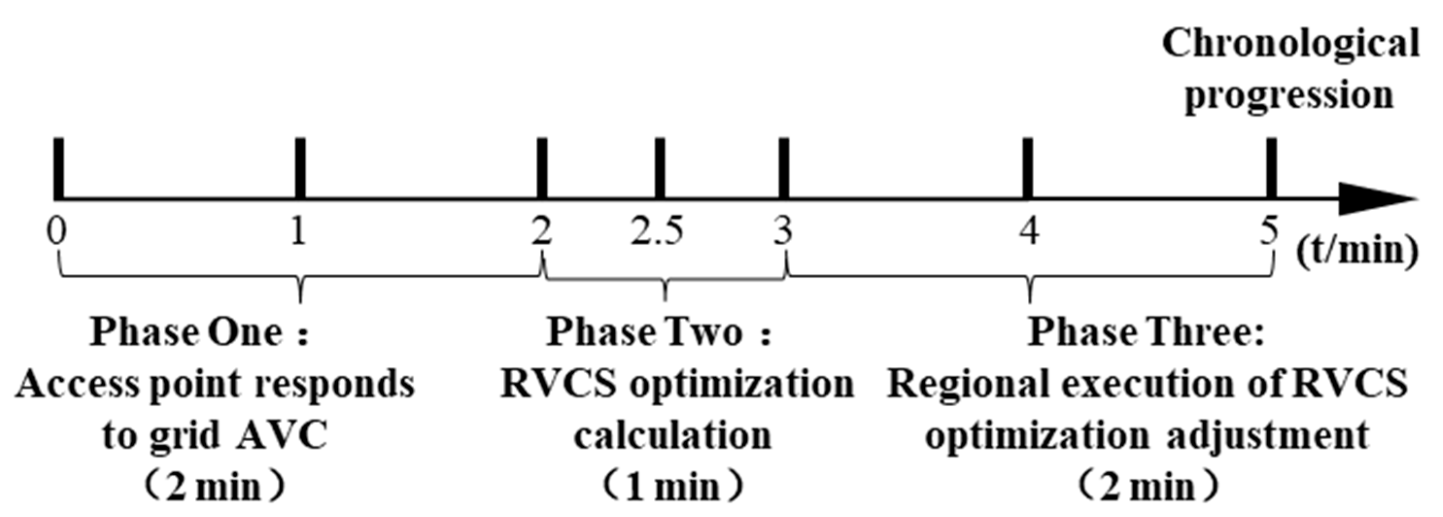
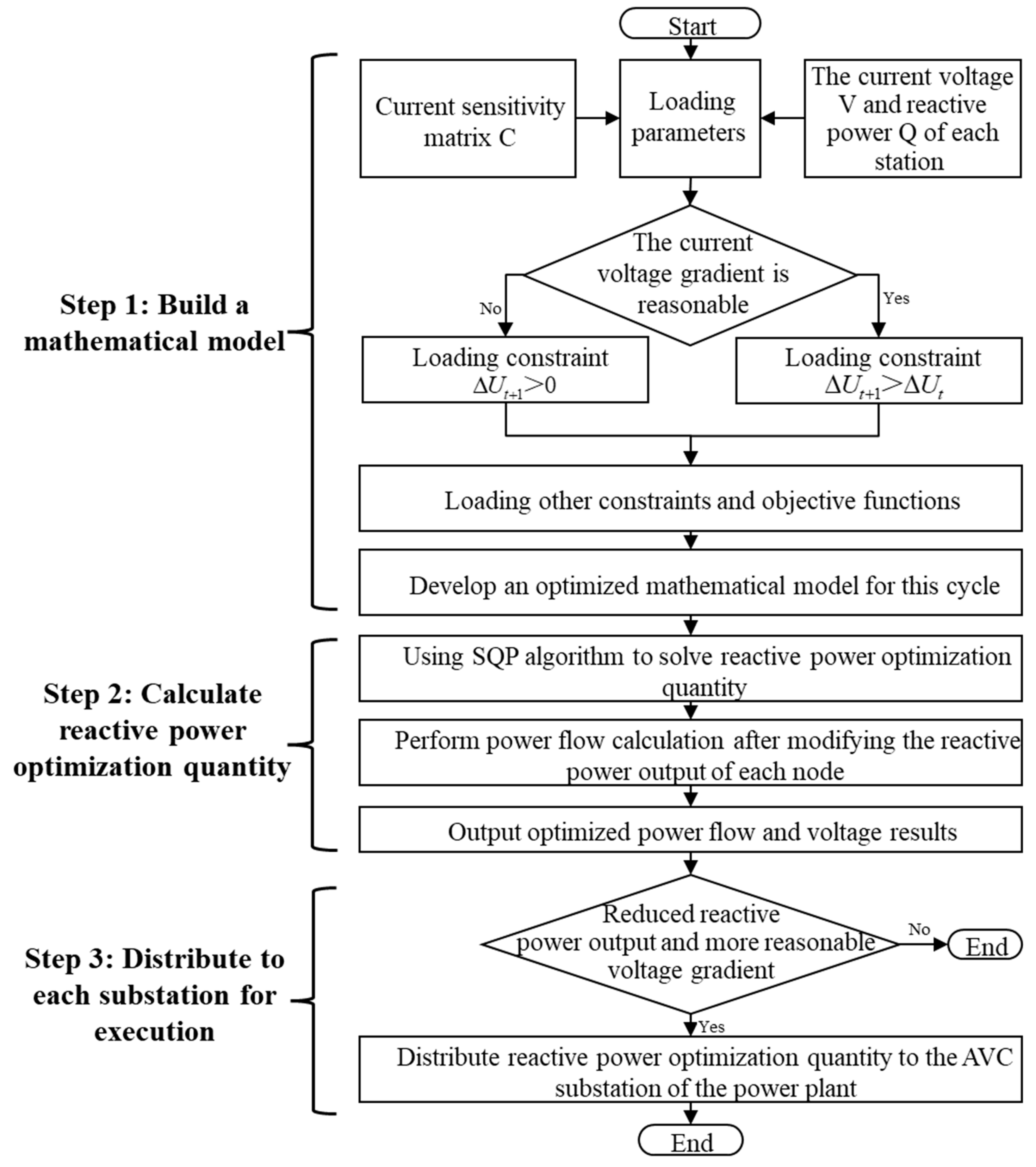
This constraint represents the maximum and minimum reactive power output of a single station.

$$Q_{n+i}^{min}\le Q_{n+i}^t+\Delta Q_{n+i}^t\le Q_{n+i}^{max}$$

(20)

where $Q_{n+i}^{max}$ and $Q_{n+i}^{min}$ denote the upper and lower limits of the reactive power output for station i. These limits correspond to the total maximum and minimum reactive power output capacities of all generators within the station.

4.3. Working Flow

The mathematical model developed in this study formulates the objective function as a nonlinear optimization function of reactive power adjustment ΔQ, characterized by high complexity, multiple constraints, and strict convergence criteria. Algorithms commonly used for solving nonlinear optimization problems include gradient descent (GD) [46], the interior-point method (IPM) [47], and sequential quadratic programming (SQP) [48]. Among these, GD is suitable for optimization problems with simple constraints but may exhibit poor convergence when handling problems with complex constraints or non-convex objective functions. The IPM is effective for large-scale problems, particularly when handling complex constraints, but incurs a high computational cost. The SQP approach decomposes the nonlinear optimization problem into a series of QP subproblems, iteratively approximating the optimal solution. This method offers rapid convergence, high efficiency, and remarkable stability. Given the complex constraints, multivariable coupling characteristics, and computational efficiency and solution stability requirements of the reactive power optimization problem in CC-HPPs, the SQP algorithm was selected in this study. Based on the computed reactive power–voltage sensitivity matrix, the optimal reactive power adjustment ΔQ for each station was determined through SQP.

Figure 7 presents the flowchart of the SQP algorithm. During each AVC cycle, the sensitivity matrix was reconstructed in real time, and initial values for the reactive power adjustment vector ΔQ₀, Lagrange multipliers λ^k, and convergence threshold ε were defined to formulate and solve the quadratic subproblem. The algorithm proceeded through line search and iterative updates of variables, including refinement of the Hessian matrix, until convergence criteria were met. The resulting output provides optimal reactive power adjustments for each station, facilitating coordinated voltage control and reducing regional reactive power interactions with high responsiveness to real-time system changes.

Figure 8 illustrates the solution process for the reactive power adjustment ΔQ at each station. At the beginning of the second phase within each control cycle, reactive power–voltage optimization for all stations was performed. Once the effectiveness of the optimized adjustment was confirmed, the results were dispatched to each station for implementation at the beginning of the third phase.

The process unfolds as follows:

Step 1: The current operational parameters of the system are collected, and the sensitivity matrix is computed using the method outlined in Section 2. The voltage gradient of the current operating state is then evaluated. Based on the results obtained, appropriate constraints are imposed to construct the mathematical model for the present adjustment cycle.

Step 2: The mathematical model for the current cycle is solved using the SQP algorithm to determine the reactive power optimization adjustment ΔQ for each station. The reactive power output of each station is then updated, and a power flow simulation is conducted to obtain the corresponding power flow and voltage results.

Step 3: The optimized power flow and voltage are compared with the current operating power flow and voltage. If an improvement is apparent, the optimized adjustment commands are dispatched to the AVC substations of each station for implementation. If no improvement is achieved, the current optimization cycle is terminated.

4.4. Key Indicators

To assess the effectiveness of the proposed strategy, two key indices are defined:

(1)

Absolute Value of the Reactive Power-Pulling Amplitude

The absolute value of reactive power-pulling flow, represented as A, reflects the intensity of reactive power pulling within the CC-HPP network. This metric quantifies the extent of reactive power generated by certain stations and absorbed by others within the network. A = 0 indicates that all stations within the CC-HPP network either generate or absorb reactive power simultaneously, indicating the absence of reactive power pulling. This is mathematically expressed as

$$A\left(Mvar\right)=\mathit{min}\left\{{\displaystyle \sum _{\begin{array}{c}x=2\\ x\ne y\end{array}}^n}{Q}_{e,x},\left|{\displaystyle \sum _{\begin{array}{c}y=2\\ y\ne x\end{array}}^n}{Q}_{a,y}\right|\right\}$$

(21)

where x and y denote the indices of power stations in the CC-HPP network, with x ≠ y indicating that a station cannot simultaneously absorb and generate reactive power. Further, Q_e,x signifies the reactive power generated by station x, and Q_a,γ represents the reactive power absorbed by station y.

(2)

Reasonable Voltage Gradient Operation Rate

In the CC-HPP network, the high-voltage bus voltage should exhibit a reasonably decreasing gradient from the terminal station to the leading (grid connection) station. The operational duration during which the voltage maintains this reasonable gradient is defined as the voltage reasonable gradient operation rate, denoted as B. The mathematical expression for B is

$$B\left(\%\right)=\left(1-{\displaystyle \frac{t}{T}}\right)\times 100\%$$

(22)

where t represents the total operational duration during which the voltage deviation remains positive, and T represents the total operational period. A value of B closer to 100% indicates a longer operational duration with a reasonable voltage gradient, which enhances the security and operational stability of the power grid.

5. Case Study

5.1. Parameter Settings and Scene Division

As displayed in Figure 9, a CC-HPP network comprising stations P, S, and Z in a river basin in Southwestern China is adopted as a case study object. Based on the physical connections and actual parameters (

Table 1. Equivalent generator parameters.

Station	Capacity (MW)	Maximum Reactive Power (MVar)	Minimum Reactive Power (MVar)	Generator Terminal Voltage (kV)
Station Z	720	349	−280	15.75
Station S	660	320	−480	15.75
Station P	3600	1746	−1500	20.00

,

Table 2. Single transformer parameters.

Transformer	Capacity (MVA)	Impedance (Ω)	Transformation Ratio
Station Z	200	0.002780 + j0.180838	15.75/550
Station S	375	0.001379 + j0.104186	15.75/550
Station P	667	0.001184 + j0.094633	20.00/550

and

Table 3. Transmission line parameters.

Line	Impedance (Ω)	Electrical Susceptance (10−6 S)	Charging Power (MVar)
Z–S Line	0.72 + j8.585	119.226	32.86
S–P Line	0.44 + j6.072	94.922	26.16
BP Line	3.27 + j50.384	744.902	205.31

) of this network, derived from the SCADA data recorded in February 2023, a power flow model is established to analyze its operational characteristics.

During the actual operation of the considered CC-HPP network, frequent reactive power-pulling phenomena have been observed when multiple stations participate in closed-loop AVC. To assess the effectiveness of the proposed control strategy, two specific operational scenarios, including significant reactive power-pulling occurrences, are selected. (1) 17 February 2023 (21:00–22:00): A period when reactive power pulling was actively occurring. (2) 19 February 2023 (11:00–12:00): A period just before the pulling commenced. A continuous power flow simulation is performed for each scenario, implementing the control strategy during the reactive power pulling in Scenario 1 and before its onset in Scenario 2. The simulation results are analyzed in terms of the effectiveness of the proposed strategy in mitigating interstation reactive power pulling and correcting the voltage gradient. This analysis validates the effectiveness of the strategy in controlling and preventing reactive power–voltage anomalies in CC-HPP networks subjected to closed-loop AVC.

5.2. Result Analysis

The simulation results confirm that the RVCS control strategy significantly suppresses reactive power pulling and improves voltage gradient stability. Notably, in cases where the RVCS is implemented before the onset of reactive power pulling (Scenario 2), the optimization effect is more pronounced.

(1)

Simulation Results for the Absolute Reactive Power Pulling Amplitude

Figure 10 presents the reactive power-pulling amplitude A for both scenarios.

In Scenario 1, between 21:00 and 21:40, approximately 60 MVar of reactive power pulling occurs. Once the RVCS is activated at 21:00, a significant reduction in reactive power pulling is observed in the first control cycle, with further improvements in subsequent cycles. In Scenario 2, between 11:15 and 12:00, approximately 50 MVar of reactive power pulling is anticipated. With the deployment of the RVCS at 11:00, two rounds of control adjustments successfully prevent major reactive power pulling instances.

To intuitively evaluate the overall regulation performance of the proposed optimization strategy during the entire simulation period, this study introduces the time-averaged reactive power pulling amplitude A_av based on A defined in Section 4.4. This index reflects the average intensity of reactive power pulling throughout the simulation period and serves as a measure of the strategy’s overall effectiveness. The calculation formula is shown in Equation (23). A comparison of the A_av results under the two simulation scenarios is presented in

Table 4. Optimization results in reactive power pulling (A_av) across simulation scenarios.

Simulation Scenario	Actual Value Aav (MVar)	Simulate Value Aav (MVar)	Percentage Decrease (%)
Scenario 1 (21:00–22:00)	39.14	3.34	91.47
Scenario 2 (11:00–12:00)	18.73	0.42	97.76

.

$$A_{av}={\displaystyle \frac{1}{K}}{\displaystyle \sum _{k=1}^K}{A}_k$$

(23)

where K represents the total number of sampled values of A during the simulation, and A_k denotes the reactive power-pulling amplitude at the tth sampling point. The relevant sampling data are presented in Appendix A as

Table A1. Reactive power output of each station in scenario 1 during simulation.

Time	Actual Value of Z Station (MVar)	Simulation Value of Z Station (MVar)	Actual Value of S Station (MVar)	Simulation Value of S Station (MVar)
21:01	−48.20	−48.20	65.41	65.41
21:02	−64.40	−47.08	89.45	68.90
21:03	−72.20	−47.03	93.95	68.86
21:04	−78.90	−23.51	101.48	34.43
21:05	−74.80	−11.76	98.58	17.22
21:06	−76.90	−12.89	129.14	11.61
21:07	−73.50	−13.52	107.11	7.23
21:08	−68.80	−13.31	109.43	8.17
21:09	−79.50	−6.66	115.12	4.09
21:10	−80.10	−3.33	117.13	2.04
21:11	−76.30	−7.52	122.80	14.30
21:12	−70.80	−6.36	100.09	14.33
21:13	−76.80	−6.38	103.02	13.94
21:14	−69.80	−3.19	91.18	6.97
21:15	−76.40	−1.59	89.68	3.48
21:16	−70.50	−7.28	88.97	−4.60
21:17	−58.90	−8.41	88.90	−21.83
21:18	−48.20	−8.64	78.53	−24.71
21:19	−64.40	−8.25	73.83	−16.25
21:20	−72.20	−5.82	56.71	−9.80
21:21	−78.90	−4.14	61.86	15.73
21:22	−74.80	−4.05	80.89	45.23
21:23	−76.90	−3.99	111.54	45.34
21:24	−73.50	3.71	122.56	28.18
21:25	−68.80	5.30	142.30	17.45
21:26	−79.50	4.76	133.81	1.39
21:27	−80.10	4.65	130.47	−18.99
21:28	−76.30	4.70	123.85	−19.00
21:29	−70.80	2.57	125.83	−9.50
21:30	−76.80	1.54	105.88	−4.74
21:31	−69.80	4.27	95.11	29.92
21:32	−76.40	4.30	96.06	68.12
21:33	−70.50	4.19	88.32	68.19
21:34	−58.90	15.58	77.99	47.05
21:35	−48.20	18.95	80.82	34.42
21:36	−64.40	17.87	70.42	−22.20
21:37	−72.20	17.92	48.53	−75.96
21:38	−78.90	17.91	31.96	−76.13
21:39	−74.80	9.08	33.86	−58.97
21:40	−76.90	4.72	9.01	−45.99
21:41	−73.50	4.22	7.27	−24.04
21:42	−68.80	5.33	0.72	−4.97
21:43	−79.50	5.21	11.77	−5.15
21:44	−80.10	2.67	−5.83	−2.57
21:45	−76.30	1.51	−14.97	−1.28
21:46	−70.80	3.98	6.65	−5.30
21:47	−76.80	3.99	−0.54	−5.14
21:48	−69.80	0.84	−3.47	−5.74
21:49	−76.40	0.42	−7.16	−2.87
21:50	−70.50	0.21	−7.50	−1.44
21:51	−58.90	−1.68	−27.14	57.32
21:52	−48.20	24.08	−27.75	85.17
21:53	−64.40	24.19	−10.67	85.40
21:54	−72.20	34.98	1.37	64.83
21:55	−78.90	37.93	−16.26	52.48
21:56	−74.80	37.64	−79.17	34.65
21:57	−76.90	37.47	−54.86	16.66
21:58	−73.50	37.58	−52.06	16.89
21:59	−68.80	27.81	−43.47	17.50
22:00	−79.50	20.69	−32.76	15.52

and

Table A2. Reactive power output of each station in scenario 2 during simulation.

Time	Actual Value of Z Station (MVar)	Simulation Value of Z Station (MVar)	Actual Value of S Station (MVar)	Simulation Value of S Station (MVar)
11:01	−12.00	−12.00	−17.22	−17.22
11:02	−19.90	−11.25	−11.11	−15.65
11:03	−23.40	−11.25	−4.29	−15.65
11:04	−27.50	−7.80	−5.93	−9.97
11:05	−27.30	−3.90	−14.28	−4.98
11:06	−12.10	−4.00	−13.84	20.29
11:07	−16.70	−2.82	−11.01	22.56
11:08	−11.50	−2.83	−14.35	22.46
11:09	−2.10	−1.20	−20.05	11.44
11:10	−9.20	−0.60	−16.94	5.72
11:11	−5.40	−2.01	−17.42	−5.39
11:12	−23.40	−5.18	−1.91	−17.12
11:13	−16.80	−5.01	4.30	−17.06
11:14	−25.50	−3.45	−3.03	−9.47
11:15	−18.40	−1.73	8.73	−4.74
11:16	−20.20	3.57	11.22	10.55
11:17	−20.80	5.51	9.62	26.15
11:18	−18.40	5.60	15.52	26.10
11:19	−25.90	6.08	21.83	12.96
11:20	−30.30	4.01	39.59	5.79
11:21	−33.30	4.31	55.24	−15.94
11:22	−43.80	2.25	57.70	−24.44
11:23	−38.00	2.34	50.03	−25.20
11:24	−35.30	−0.01	50.71	−13.78
11:25	−40.80	0.00	54.36	−6.89
11:26	−47.40	1.14	62.51	2.74
11:27	−45.40	1.22	62.81	2.68
11:28	−41.00	1.04	59.92	2.55
11:29	−51.60	0.52	60.67	1.27
11:30	−47.80	0.26	63.12	0.64
11:31	−51.10	0.89	43.96	2.25
11:32	−55.10	0.89	37.48	2.19
11:33	−49.30	0.89	34.00	2.13
11:34	−53.00	0.45	28.85	1.07
11:35	−49.10	0.22	25.07	0.53
11:36	−40.40	1.29	15.96	2.94
11:37	−37.10	1.29	6.28	3.00
11:38	−32.50	1.29	4.37	3.00
11:39	−36.90	0.65	−11.59	1.50
11:40	−31.70	0.32	−9.95	0.75
11:41	−27.20	2.77	−12.71	−17.51
11:42	−31.60	1.10	1.33	−26.38
11:43	−36.90	1.10	−1.60	−26.38
11:44	−36.50	−1.23	2.36	−14.97
11:45	−37.60	−0.61	−0.20	−7.49
11:46	−39.00	3.00	−11.35	47.53
11:47	−35.30	10.75	1.61	74.31
11:48	−40.70	10.84	9.62	74.32
11:49	−41.20	22.02	17.26	53.22
11:50	−46.20	25.17	43.31	40.57
11:51	−46.10	21.68	38.71	26.40
11:52	−52.00	23.58	41.33	3.42
11:53	−41.80	26.54	34.38	3.43
11:54	−44.10	16.12	33.39	4.57
11:55	−40.80	8.64	33.35	2.86
11:56	−50.30	8.40	27.90	2.29
11:57	−55.70	8.40	27.18	2.34
11:58	−55.30	8.51	29.06	2.53
11:59	−56.30	4.26	24.59	1.27
12:00	−53.10	2.13	36.93	0.63

.

The simulation results show that deploying the RVCS after the onset of reactive power pulling can effectively suppress the phenomenon within one to two control cycles and maintain a low pulling level thereafter. In contrast, proactive deployment of the RVCS before onset can prevent the occurrence of reactive power pulling, leading to better operational performance overall than that of reactive correction.

(2)

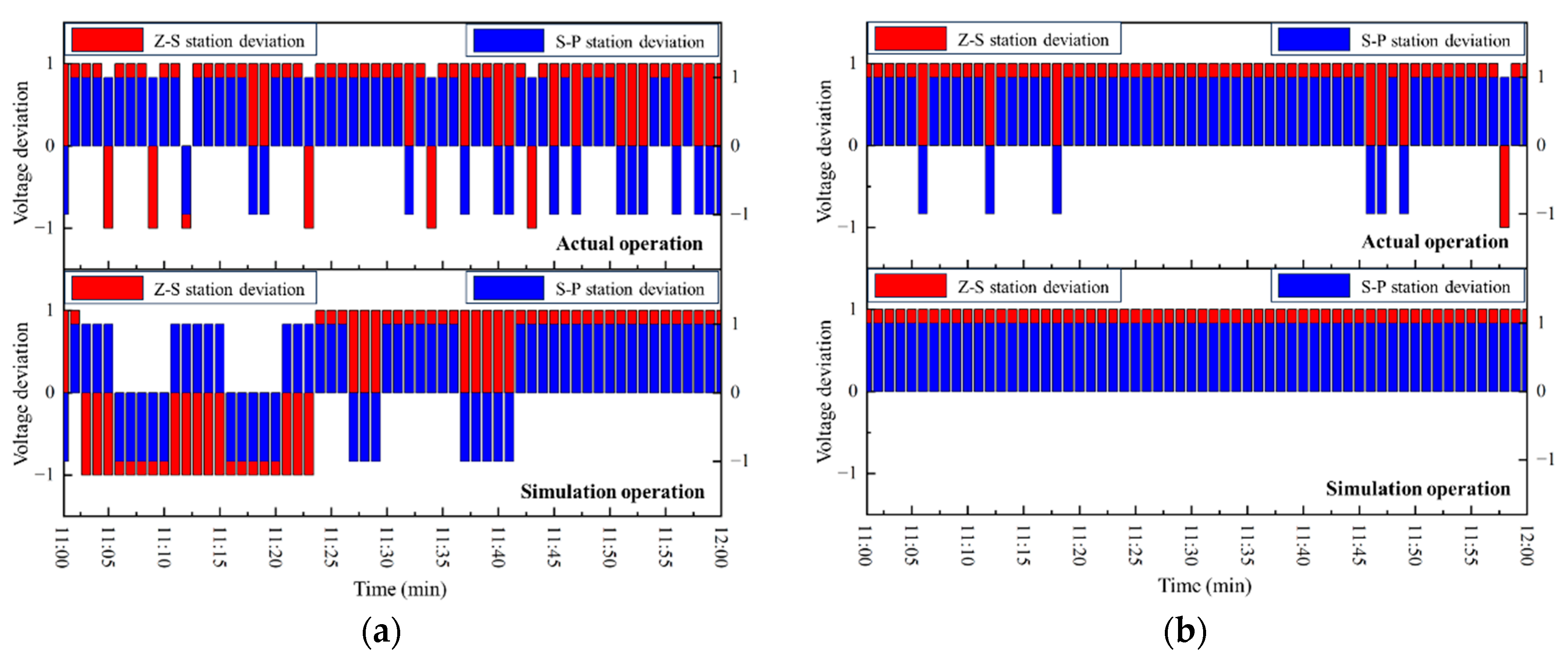
Simulation Results for the Reasonable Voltage Gradient Operation Rate

Figure 11 presents the voltage deviation over time for both simulation scenarios.

In Scenario 1, during the first 30 min, voltage gradients fluctuate substantially owing to reactive power pulling. However, after multiple optimization cycles, the system stabilizes. Meanwhile, in Scenario 2, voltage gradients remain stable throughout the period, preventing large reactive power oscillations.

Table 5. Comparison between simulated and actual voltage reasonable gradient operation rate (B).

Simulation Scenario		Actual Operation B (%)	Simulated Operation B (%)	Percentage Increase (%)
Scenario 1	Period 1 (21:00–21:30)	86.67	41.67	−45.00
	Period 2 (21:30–22:00)	75.00	91.67	16.67
Scenario 2	Period 1 (11:00–11:30)	95.00	100.00	5.00
	Period 2 (11:30–12:00)	93.33	100.00	6.67

compares simulated and actual values for the voltage reasonable gradient operation rate (B) in each scenario.

The simulation results indicate that, when the RVCS is deployed after the onset of reactive power pulling, correcting the voltage gradient typically requires multiple consecutive control cycles, during which temporary voltage gradient deviations may occur. In contrast, proactive deployment of the RVCS before onset allows for the more effective control and maintenance of a reasonable voltage gradient.

(3)

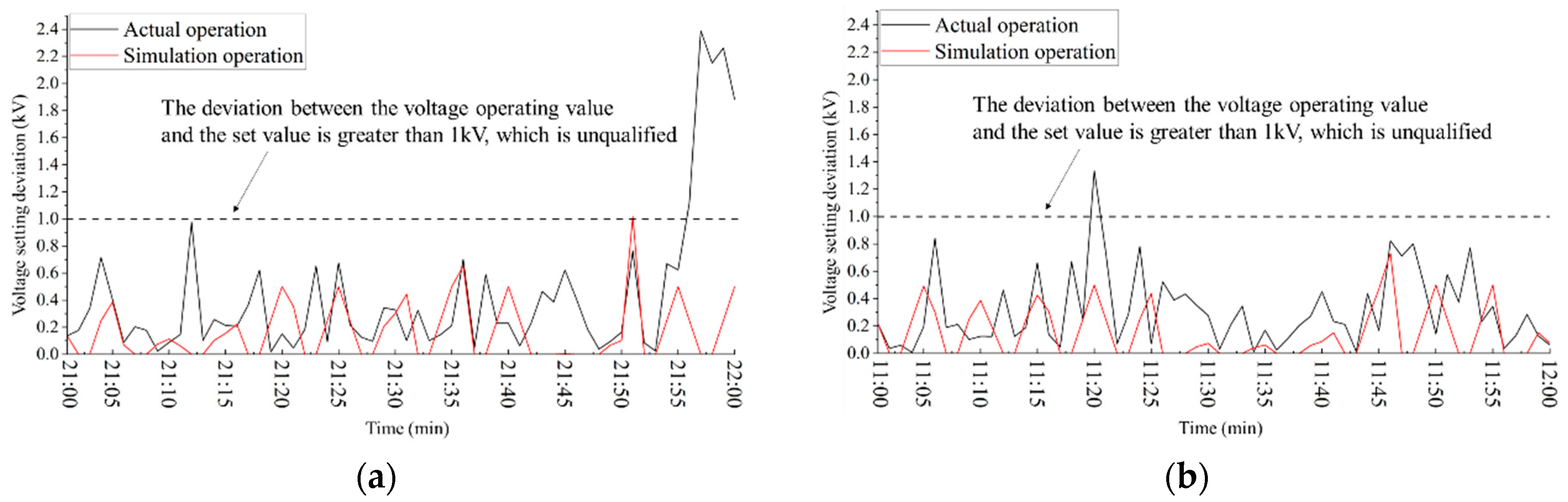
Simulation Results for AVC Qualification Rate

Figure 12 presents the deviation between the voltage operating value and set value.

When the voltage deviation is greater than 1 kV, it is judged as an unqualified point. The ratio of qualified points to issued points is recorded as the qualification rate. In scenario 1, there are a total of five non-conforming points during actual operation, while there is only one non-conforming point during simulation operation. Meanwhile, in scenario 2, there is only one non-conforming point during actual operation, and all voltages are qualified during simulation operation.

Table 6. Comparison between simulated and actual AVC qualification rate.

Simulation Scenario	Actual Qualification Points	Simulated Qualification Points	Actual Qualification Rate	Simulated Qualification Rate
Scenario 1 (21:00–22:00)	5	1	91.66%	98.33%
Scenario 2 (11:00–12:00)	1	0	98.33%	100.00%

compares simulated and actual values for the AVC qualification rate in each scenario.

The simulation results in both scenarios indicate that the proposed strategy has varying degrees of improvement in the qualification rate of chain hydropower AVC response.

In summary, based on the above analysis, the collaborative response strategy effectively mitigates the problem of reactive power pulling, improves the voltage gradient rationality, and enhances the AVC qualification rate. Compared to the traditional AVC strategy, the proposed method enables more coordinated multi-station voltage control, ensuring a more stable and efficient reactive power distribution across the CC-HPP network.

6. Conclusions and Discussion

6.1. Conclusions

To minimize reactive power pulling and abnormal voltage gradients in CC-HPP networks during closed-loop AVC, this study proposes a collaborative response optimization strategy based on reactive power–voltage sensitivity analysis. Our key findings include

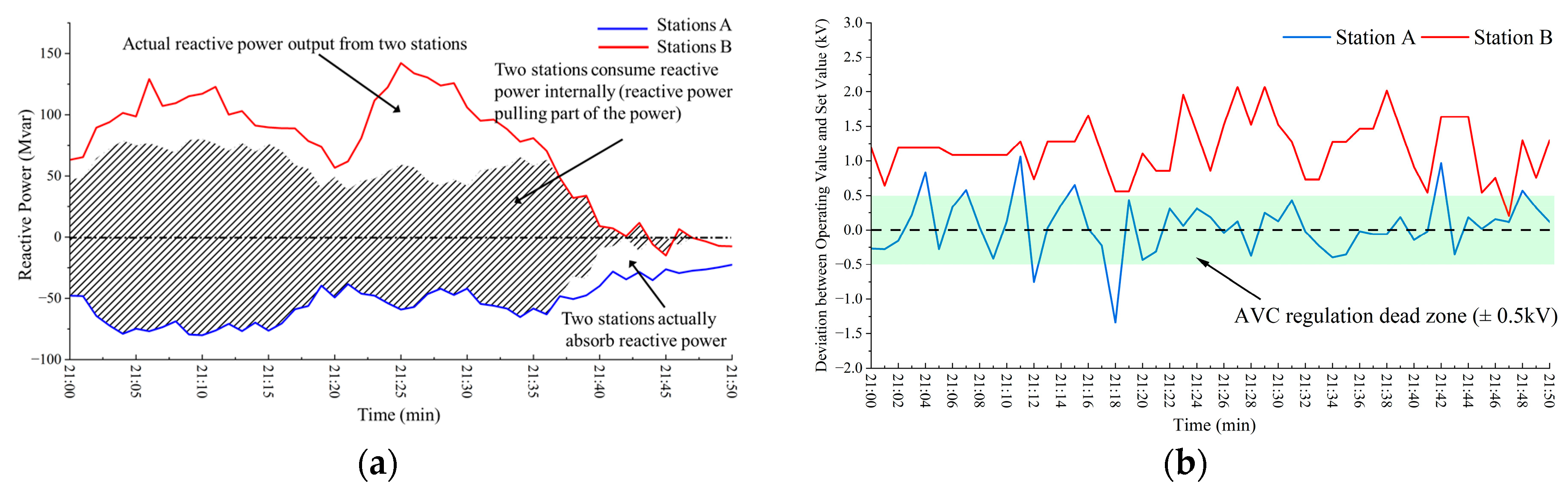
• In a cascade hydropower system, when transferred reactive power causes bus voltage deviations surpassing the AVC dead band, counter-responses from AVC substations may trigger reactive power–voltage anomalies across the entire CC-HPP network.
• Compared to traditional two-stage voltage control, the proposed RVCS accounts for interstation interactions within the network. While ensuring compliance with grid reactive power requirements, it also boosts the power factor performance of regional hydropower stations.
• In optimized simulations, early RVCS implementation prevents reactive power pulling and maintains a reasonable voltage gradient. However, if corrective measures are applied after the onset of reactive power pulling, multiple adjustment cycles are required for system stabilization.

6.2. Discussion

While this study proposes a sensitivity-based coordinated response optimization strategy and demonstrates its effectiveness through simulation and real-world data analysis, several limitations persist. First, the simulation validation is confined to two operational scenarios, lacking comprehensive coverage of cases such as seasonal changes, reservoir operations, and conditions involving complex renewable energy integration. Second, the optimization method is primarily based on deterministic modeling and a single coordination framework, without incorporating comparative analyses or integration with other advanced control strategies. Third, the proposed approach depends entirely on real-time feedback and lacks the predictive capability to anticipate future system variations. To overcome these limitations and enhance the practical relevance and scalability of the strategy, future research will explore the following directions:

• Adaptability Analysis under Multi-Scenario and Renewable-Integrated Conditions: To enhance the applicability of the proposed strategy, future research will evaluate its adaptability across a range of hydropower operation scenarios, including reservoir regulation, intra-day peak-shaving, fluctuating load levels, and seasonal variations in water availability during wet and dry periods. In addition, this study explores the reactive power coordination mechanism of hydropower under hybrid configurations with renewable sources (e.g., PV integration), aiming to enhance the strategy’s applicability in complex source-load coupled systems. Qiu et al.’s work on the real-time scheduling of cascaded run-of-river hydro plants provides a useful reference for such hybrid operation control [49].
• Exploration of Alternative Coordinated Control Methods in CC-HPPs: Future work will explore the applicability of alternative coordinated control frameworks in chain-structured hydropower systems, including model predictive control (MPC), distributed optimization, and deep learning-based approaches. Given the unique hierarchical structure and heterogeneous control objectives of CC-HPPs, future work should evaluate how these advanced methods can be tailored and implemented for multi-station reactive power regulation. Notable references include the cascaded PID controller model for hybrid energy systems by Behera et al. [50] and the ML-enhanced Benders decomposition proposed by Borozan et al. [51].
• Forecast-aided Coordinated Control Enhancement: To improve proactive control capabilities, future work will investigate the integration of machine learning-based forecasting techniques into the strategy. By predicting the evolving system state, including voltage profiles and dynamic reactive power demands, forecast-aided optimization may significantly improve control precision and responsiveness. The forecasting framework proposed by Giannelos et al. [52], which ensures high prediction accuracy through a structured modeling process, offers practical guidance in this direction.

References

1. Kougias, I.; Aggidis, G.; Avellan, F.; Deniz, S.; Lundin, U.; Moro, A.; Muntean, S.; Novara, D.; Pérez-Díaz, J.I.; Quaranta, E. Analysis of emerging technologies in the hydropower sector. Renew. Sustain. Energy Rev. 2019, 113, 109257. [Google Scholar] [CrossRef]
2. Azimov, U.; Avezova, N. Sustainable small-scale hydropower solutions in Central Asian countries for local and cross-border energy/water supply. Renew. Sustain. Energy Rev. 2022, 167, 112726. [Google Scholar] [CrossRef]
3. Quaranta, E.; Bejarano, M.D.; Comoglio, C.; Fuentes-Pérez, J.F.; Pérez-Díaz, J.I.; Sanz-Ronda, F.J.; Schletterer, M.; Szabo-Meszaros, M.; Tuhtan, J.A. Digitalization and real-time control to mitigate environmental impacts along rivers: Focus on artificial barriers, hydropower systems and European priorities. Sci. Total Environ. 2023, 875, 162489. [Google Scholar] [CrossRef] [PubMed]
4. Xiang, W. A brief discussion on voltage joint regulation of waterfall gully, Shenxigou, and pillow dam hydropower stations. Sichuan Hydroelectr. Power Gener. 2021, 2, 137–142. [Google Scholar]
5. Wang, J.; Wang, L.; Yang, J.; Huang, E.; Zhang, L.; Liu, X.; Yang, K. Simulation analysis of reactive power and voltage for chain-structured cascade hydropower stations. J. Xihua Univ. (Nat. Sci. Ed.) 2025, 44, 1–9. [Google Scholar]
6. Chou, M.H.; Su, C.L.; Lee, Y.C.; Chin, H.M.; Parise, G.; Chavdarian, P. Voltage-drop calculations and power cable designs for harbor electrical distribution systems with high voltage shore connection. IEEE Trans. Ind. Appl. 2016, 53, 1807–1814. [Google Scholar] [CrossRef]
7. Thakur, R.; Chawla, P. Voltage drop calculations & design of urban distribution feeders. Int. J. Res. Eng. Technol. 2015, 4, 43–53. [Google Scholar]
8. Hualiang, L.; Min, S.; Di, S.; Lei, Z.; Xiaozhen, J. Research on voltage drop of test transformer during combined voltage test. In Proceedings of the 16th IET International Conference on AC and DC Power Transmission (ACDC 2020), Online Conference, 2–3 July 2020. [Google Scholar]
9. Khadka, S.; Wagle, A.; Dhakal, B.; Gautam, R.; Nepal, T.; Shrestha, A.; Gonzalez-Longatt, F. Agglomerative hierarchical clustering methodology to restore power system considering reactive power balance and stability factor analysis. Int. Trans. Electr. Energy Syst. 2024, 2024, 8856625. [Google Scholar] [CrossRef]
10. Liu, B. The application of electrical engineering automation technology in the operation of power systems. Light. Source Illum. 2024, 12, 201–203. [Google Scholar]
11. Dey, R.; Nath, S. A new active and reactive power control strategy for multifrequency microgrid in islanded mode. In Proceedings of the 2021 5th International Conference on Smart Grid and Smart Cities (ICSGSC), Tokyo, Japan, 18–20 June 2021. [Google Scholar]
12. Sadeghi, S.E.; Akbari Foroud, A. A general index for voltage stability assessment of power system. Int. Trans. Electr. Energy Syst. 2021, 31, e13155. [Google Scholar] [CrossRef]
13. Sahu, A.; Davis, K. Bayesian reinforcement learning for automatic voltage control under cyber-induced uncertainty. arXiv 2023, arXiv:2305.16469. [Google Scholar] [CrossRef]
14. Yin, L.; Zhang, C.; Wang, Y.; Gao, F.; Yu, J.; Cheng, L. Emotional deep learning programming controller for automatic voltage control of power systems. IEEE Access 2021, 9, 31880–31891. [Google Scholar] [CrossRef]
15. Lu, Z.; Zhao, G.; Kong, X.; Chen, J.; Guo, X.; Zhang, J. A detection based on particle filtering and multivariate time-series anomaly detection via graph attention network for automatic voltage control attack in smart grid. Sustain. Energy Grids Netw. 2024, 40, 101494. [Google Scholar] [CrossRef]
16. Guo, Q.; Sun, H.; Zhang, B.; Wu, W.; Li, Q. Research on coordinated secondary voltage control. Power Syst. Autom. 2005, 29, 19–24. [Google Scholar]
17. Tang, M.; Pang, X.; Li, M.; Liu, B.; Yin, X.; Zhang, B. Research and implementation plan of provincial local integration AVC system taking into account cascade hydropower stations. Power Autom. Equip. 2009, 29, 119–123. [Google Scholar]
18. Wang, L.; Wang, J.; Zhang, L.; Yang, J.; Tang, Y.; Huang, E.; Liu, X. Research on automatic voltage control for chain-structured hydropower stations. In Proceedings of the 2023 3rd International Conference on Energy Engineering and Power Systems (EEPS), Dali, China, 28–30 July 2023. [Google Scholar]
19. Wu, H.; Zhang, L.; Shu, A. Research on countermeasures for large hydropower plants participating in the ‘two regulations’ under asynchronous networking. Yunnan Hydrop. 2020, 8, 236–238. [Google Scholar]
20. Yang, M.; Wu, B.; Yu, T. The application of weighted average algorithm in automatic voltage control system of hydropower station. Inn. Mong. Electr. Power Technol. 2023, 41, 7–13. [Google Scholar]
21. Schwenzer, M.; Ay, M.; Bergs, T.; Abel, D. Review on model predictive control: An engineering perspective. Int. J. Adv. Manuf. Technol. 2021, 117, 1327–1349. [Google Scholar] [CrossRef]
22. Molzahn, D.K.; Dörfler, F.; Sandberg, H. A survey of distributed optimization and control algorithms for electric power systems. IEEE Trans. Smart Grid 2017, 8, 2941–2962. [Google Scholar] [CrossRef]
23. Mathew, A.; Amudha, P.; Sivakumari, S. Deep learning techniques: An overview. In Smart Intelligent Computing and Applications; Springer: Singapore, 2020; Volume 1141, pp. 599–608. [Google Scholar]
24. Peschon, J.; Piercy, D.S.; Tinney, W.F.; Tveit, O.J. Sensitivity in power systems. IEEE Trans. Power Appar. Syst. 1968, 87, 1687–1696. [Google Scholar] [CrossRef]
25. Kasturi, R.; Dorraju, P. Sensitivity analysis of power systems. IEEE Trans. Power Appar. Syst. 1969, 88, 1521–1529. [Google Scholar] [CrossRef]
26. Lotufo, A.D.P.; Lopes, M.L.M.; Minussi, C.R. Sensitivity analysis by neural networks applied to power systems transient stability. Electr. Power Syst. Res. 2007, 77, 730–738. [Google Scholar] [CrossRef]
27. Ni, F.; Nijhuis, M.; Nguyen, P.H.; Cobben, J.F.G. Variance-based global sensitivity analysis for power systems. IEEE Trans. Power Syst. 2017, 33, 1670–1682. [Google Scholar] [CrossRef]
28. Ginocchi, M.; Ponci, F.; Monti, A. Sensitivity analysis and power systems: Can we bridge the gap? A review and a guide to getting started. Energies 2021, 14, 8274. [Google Scholar] [CrossRef]
29. Wang, H.; Hou, K.; Liu, X.; Yu, X.; Jia, H.; Du, J. A method for enhancing the resilience of electrical interconnection systems based on global sensitivity analysis. Power Syst. Autom. 2023, 47, 59–67. [Google Scholar]
30. Schyska, B.U.; Kies, A.; Schlott, M.; Von Bremen, L.; Medjroubi, W. The sensitivity of power system expansion models. Joule 2021, 5, 2606–2624. [Google Scholar] [CrossRef]
31. Wang, C.; Feng, C.; Zeng, Y.; Zhang, F. Improved correction strategy for power flow control based on multi-machine sensitivity analysis. IEEE Access 2020, 8, 82391–82403. [Google Scholar] [CrossRef]
32. Sun, H.; Guo, Q.; Zhang, B.; Li, Y.; Li, Q.; Wu, L.; Yu, Z. Automatic voltage control scheme for large-scale power networks. Power Grid Technol. 2006, 30, 13–18. [Google Scholar]
33. Naresh, D. A distributed AC power grid with wind farms using ADMM-based active and reactive power control. Int. J. Eng. Sci. Adv. Technol. 2021, 23, 31–36. [Google Scholar]
34. Yang, J.; Zhu, S.; Zhou, T. Distributed model predictive control for voltage coordination of distributed photovoltaic networks. J. Appl. Sci. Eng. 2023, 28, 1341–1350. [Google Scholar]
35. Hamrouni, N.; Younsi, S.; Jraidi, M. A flexible active and reactive power control strategy of a LV grid connected PV system. Energy Proced. 2019, 162, 325–338. [Google Scholar] [CrossRef]
36. Wu, Y.; Shang, B.; Yang, P.; Yang, L.; Yu, B.; Ma, T.; Qiao, J. Research on reactive power circulation suppression strategy for new energy clusters. Inn. Mong. Electr. Power Technol. 2023, 4, 13–19. [Google Scholar]
37. Wang, B.; Guo, Q.; Sun, H.; Tang, L.; Zhang, B.; Wu, W. Research and practice on automatic voltage control of ultra high voltage near area power grid. Power Syst. Autom. 2013, 37, 99–105. [Google Scholar]
38. Yu, H. Research on Optimal Method of Reactive Voltage Control for UHV Power Network. Mod. Ind. Econ. Informaionization 2024, 245, 261–262+267. [Google Scholar]
39. Shi, X.; Wang, B.; Chen, P. Application of Coordinating Technology between Power Plants in Automatic Voltage Control System of Power Plants Near UHV Grid. Shanxi Electr. Power 2013, 183, 1–5. [Google Scholar]
40. Wang, B.; Guo, Q.; Sun, H.; Tang, L.; Zhang, B.; Tian, J. Coordinated control method for strong coupling power plants in automatic voltage control. Power Syst. Autom. 2015, 12, 165–171. [Google Scholar]
41. Han, B.; Wang, B.; Dai, F.; Wang, D.; Qin, J.; Wang, L. Research on automatic voltage control of power grid considering safety voltage constraints of large power grid. Electr. Meas. Instrum. 2020, 57, 6–11. [Google Scholar]
42. Ibe, O.G.; Onyema, A.I. Concepts of reactive power control and voltage stability methods in power system network. IOSR J. Comput. Eng. 2013, 11, 15–25. [Google Scholar]
43. Begovic, M.M.; Phadke, A.G. Control of voltage stability using sensitivity analysis. IEEE Trans. Power Syst. 1992, 7, 114–123. [Google Scholar] [CrossRef]
44. Gomes, F.V.; Carneiro, S.; Pereira, J.L.R.; Vinagre, M.P.; Garcia, P.A.N.; De Araujo, L.R. A new distribution system reconfiguration approach using optimum power flow and sensitivity analysis for loss reduction. IEEE Trans. Power Syst. 2006, 21, 1616–1623. [Google Scholar] [CrossRef]
45. Li, Y.; Wang, K.; Wang, D.; Zhu, H.; Wu, X. Fast VCA method for full dimensional sensitivity matrix considering weak coupling relationship. Electr. Meas. Instrum. 2022, 59, 69–76. [Google Scholar]
46. Li, Y.; Wang, D.; Zhang, Q.; Du, J.; Wang, Q.; Wang, Q. Gradient descent based dynamic optimization for VSG dominated microgrid. J. Eng. 2024, 2024, e70040. [Google Scholar] [CrossRef]
47. Long, G.; Wu, X.; Liu, H.; Lou, H.; Shen, B.; Yan, C.; Kong, W. Interior-point-method-based switching angle computation for selective harmonic elimination in high-frequency cascaded H-bridge multilevel inverters. J. Power Electron. 2024, 24, 1229–1240. [Google Scholar] [CrossRef]
48. Hasan, M.S.; Chowdhury, M.M.-U.-T.; Kamalasadan, S. Sequential quadratic programming (SQP) based optimal power flow methodologies for electric distribution system with high penetration of DERs. IEEE Trans. Ind. Appl. 2024, 60, 4810–4820. [Google Scholar] [CrossRef]
49. Qiu, Y.; Lin, J.; Liu, F.; Song, Y.; Chen, G. Stochastic online generation control of cascaded run-of-the-river hydropower for mitigating solar power volatility. IEEE Trans. Power Syst. 2020, 35, 4709–4722. [Google Scholar] [CrossRef]
50. Behera, A.; Panigrahi, T.K.; Ray, P.K. A novel cascaded PID controller for automatic generation control analysis with renewable sources. IEEE/CAA J. Autom. Sin. 2019, 6, 1438–1451. [Google Scholar] [CrossRef]
51. Borozan, S.; Giannelos, S.; Falugi, P.; Moreira, A. Machine learning-enhanced Benders decomposition approach for the multi-stage stochastic transmission expansion planning problem. Electr. Power Syst. Res. 2024, 237, 110895. [Google Scholar] [CrossRef]
52. Giannelos, S.; Moreira, A.; Papadaskalopoulos, D.; Strbac, G. A machine learning approach for generating and evaluating forecasts on the environmental impact of the buildings sector. Energies 2023, 16, 2915. [Google Scholar] [CrossRef]
Figure 1. Schematic representation of a typical CC-HPP network.
Energies 18 02681 g001
Figure 2. Operating parameters of a CC-HPP network: (a) operating reactive power and (b) deviation of the operating voltage from the reference voltage.
Energies 18 02681 g002
Figure 3. Equivalent circuit of a CC-HPP network.
Energies 18 02681 g003
Figure 4. Calculation process for the sensitivity matrix incorporating PV nodes.
Energies 18 02681 g004
Figure 5. Schematic of the collaborative integrated AVC mode for CC-HPPs.
Energies 18 02681 g005
Figure 6. Collaborative control timing diagram.
Energies 18 02681 g006
Figure 7. SQP algorithm flowchart.
Energies 18 02681 g007
Figure 8. RVCS optimization workflow diagram.
Energies 18 02681 g008
Figure 9. Three-station cascade hydropower flow model diagram.
Energies 18 02681 g009
Figure 10. Comparison of the reactive power-pulling amplitude across simulation scenarios: (a) RVCS activated during reactive power pulling. (b) RVCS activated before the onset of reactive power pulling.
Energies 18 02681 g010
Figure 11. Comparison of voltage deviations across simulation scenarios: (a) RVCSs activated during reactive power pulling. (b) RVCS activated before the onset of reactive power pulling.
Energies 18 02681 g011
Figure 12. Comparison of the deviation between the voltage operating value and the set value: (a) RVCS activated during reactive power pulling. (b) RVCS activated before the onset of reactive power pulling.
Energies 18 02681 g012