1. Introduction
Geometric simplicity, the absence of windings or permanent magnets on the moving part, lower manufacturing costs, greater reliability and robustness compared to other electrical machines are the main characteristics of switched reluctance machines (SRM) [
1,
2]. As the windings are not located on the moving part but only on the stator of the machine, cooling is facilitated, as the moving part does not heat up due to copper losses. The SRM has no permanent magnets or windings on the moving part, which simplifies the design, but unlike most other electrical machines, it requires a power converter. The lack of permanent magnets and windings on the rotor allows efficient operation at high speeds and high temperatures, but also brings many challenges, such as high torque ripple, noise, and vibration. It is possible to mitigate these issues by using different algorithms to control the machine with the power converter. A system with an SRM requires precise knowledge of the rotor position in order to magnetize the phases in time. Due to its simple design, an SRM is cheaper to manufacture than other electrical machines. Also, it should bear in mind that the final price of a product also includes the price of the power converter and very often the price of the incremental encoder.
SRMs are usually designed for rotary motion, although they can also be designed for linear motion [
3,
4]. SRMs designed for circular motion consist of a stator and a rotor, both of which have salient poles. The number of poles on the stator and rotor is usually not identical. Each of the stator poles has a winding, while the rotor poles are not wound.
The conventional SRM model is based on the assumption that the individual phases of the machine are magnetically decoupled from each other. The starting point is therefore the voltage equation of one phase of the machine, whereby mutual coupling effects, remanent magnetic flux, iron losses, and stray losses are neglected. The models of all individual phases of the machine result in the overall SRM model. To create such a model, it is necessary to know the resistance of the phase windings and the magnetic characteristics of the machine. The resistance can be measured relatively easily, while the magnetic characteristics require knowledge of the flux-linkage or phase inductance for different values of phase currents and rotor positions. They can be determined using the finite element method (FEM) [
5,
6,
7,
8,
9] or experimentally [
10,
11,
12]. According to [
13], there are five methods that can be used to experimentally determine the magnetic characteristics of SRMs: the direct current (DC) excitation method, the alternating current (AC) method, the AC superposition method, the current interruption method, the chopped current method, and the torque method. The DC method is satisfactorily accurate and simple, which is why it is widely used. The dependence of the phase flux-linkage or inductance on the phase current and rotor position is usually written as a second-order partial sum of the Fourier series [
7,
14]. In addition, it is possible to write them with other equations [
15], store them in a look-up table [
16] or map them with a neural network [
17,
18,
19]. It is also possible to calculate the flux-linkage using the FEM in each iteration of the program to determine the current values of the SRM variables [
20].
In most models, the iron losses are neglected, although they can account for up to 50% [
21] or up to 33% [
22] of the SRM losses. If the characteristics of the material of which the machine is made are known, it is possible to calculate the magnetic field with FEM and determine the iron losses [
22,
23]. In [
11,
24], it was proposed to improve the SRM model by introducing an equivalent resistance parallel to the phase inductance and thus modeling the iron losses without knowing the material characteristics.
In most papers, the effect of mutual coupling between the SRM phases is neglected. Nevertheless, models were created in [
8,
9,
10,
14] that take mutual coupling into account. In [
10], it was shown that the effect of mutual coupling can lead to asymmetries between the phase currents. Furthermore, this paper does not consider the time derivative of the mutual flux-linkage, but only the magnitude of the mutual flux-linkage. In [
8,
9,
14], the FEM was used to calculate the mutual coupling effect. This method requires knowledge of the detailed geometry of the machine and the material properties, i.e., data that is not publicly available and must be obtained from the manufacturer. Since a considerable part of the flux-linkage of a phase is coupled via the poles of the neighboring phases, it is necessary to consider the effect of mutual coupling in the SRM model in order to calculate the instantaneous values of the phase currents, the flux-linkages, the electromagnetic torque of the SRM, etc., more accurately. When an SRM phase is magnetized in the same/opposite direction as the neighboring phase, the flux-linkage of the neighboring phase coupled by the phase under consideration is subtracted/added from the flux-linkage generated by the phase under consideration. It is desirable to achieve a configuration in which the flux-linkage of the neighboring phase is added to the flux-linkage of the considered phase because then the flux-linkages of all phases are symmetrical. This can be achieved if each phase of the machine is magnetized in the opposite direction to the neighboring phases. Such a configuration can be achieved with an SRM that has an odd number of phases.
The remanent magnetic flux was neglected in all earlier publications. In [
25], it was pointed out that the remanent magnetic flux is important and difficult to predict and model, and the need for further research was pointed out.
SRM is considered for the operation of generators in different areas. It is used for operation in wind turbines [
26,
27,
28], as an electric starter and generator in the aerospace industry [
29], and as a generator in wave power plants [
30]. One of the main advantages of the switched reluctance generator (SRG) is that it can operate over a wide speed range and does not require a gearbox. The commercial application of the SRM was achieved in a 20 kW wind turbine [
31]. In the aerospace industry, reliability in the event of failure is emphasized as an advantage. For example, if one phase fails, the other phases can continue to generate power so that the aircraft’s electrical systems continue to be supplied with electrical energy despite the failure.
In this paper, a new model of a four-phase SRG with mutual coupling of the neighboring phases, remanent magnetic flux and iron losses is presented. To model the mutual coupling between neighboring phases, an experimental approach similar to [
10] was used, with the difference that in this paper both the magnitude of the mutual flux-linkage and its time derivative were considered. The proposed model requires only input data that can be obtained using the DC excitation method and does not require knowledge of the SRG material properties. The iron losses were calculated using the same equivalent circuit as in [
11,
24], with the difference that the equivalent resistance of the iron losses does not need to be known, but the SRG phase current component responsible for these losses was determined directly from a look-up table, which makes the advanced SRG model simpler. The remanent magnetic flux of the SRG was modeled for the first time and the induced EMS caused by it was included in the advanced SRG model. The accuracy of this model was experimentally verified in single-pulse operation and the justification for using the model was determined by comparison with the conventional SRG model. In this paper, the SRG is connected to the asymmetric bridge converter required for proper phase magnetization. The stray losses of the SRG are neglected. The mechanical losses are also not considered in the machine model itself. However, to obtain the experimental electromagnetic torque, these losses are subtracted from the measured mechanical torque. The resulting experimental electromagnetic torque, multiplied by the rotor speed, corresponds to the experimentally determined input power
Pin,exp.
2. Control of the Switched Reluctance Generator
Figure 1 shows the cross-section of the SRG with eight poles on the stator and six poles on the rotor (8/6) with the rotor at the aligned position (
Figure 1a) and unaligned position (
Figure 1b). The magnetized phase winding and its flux-linkage lines are colored red.
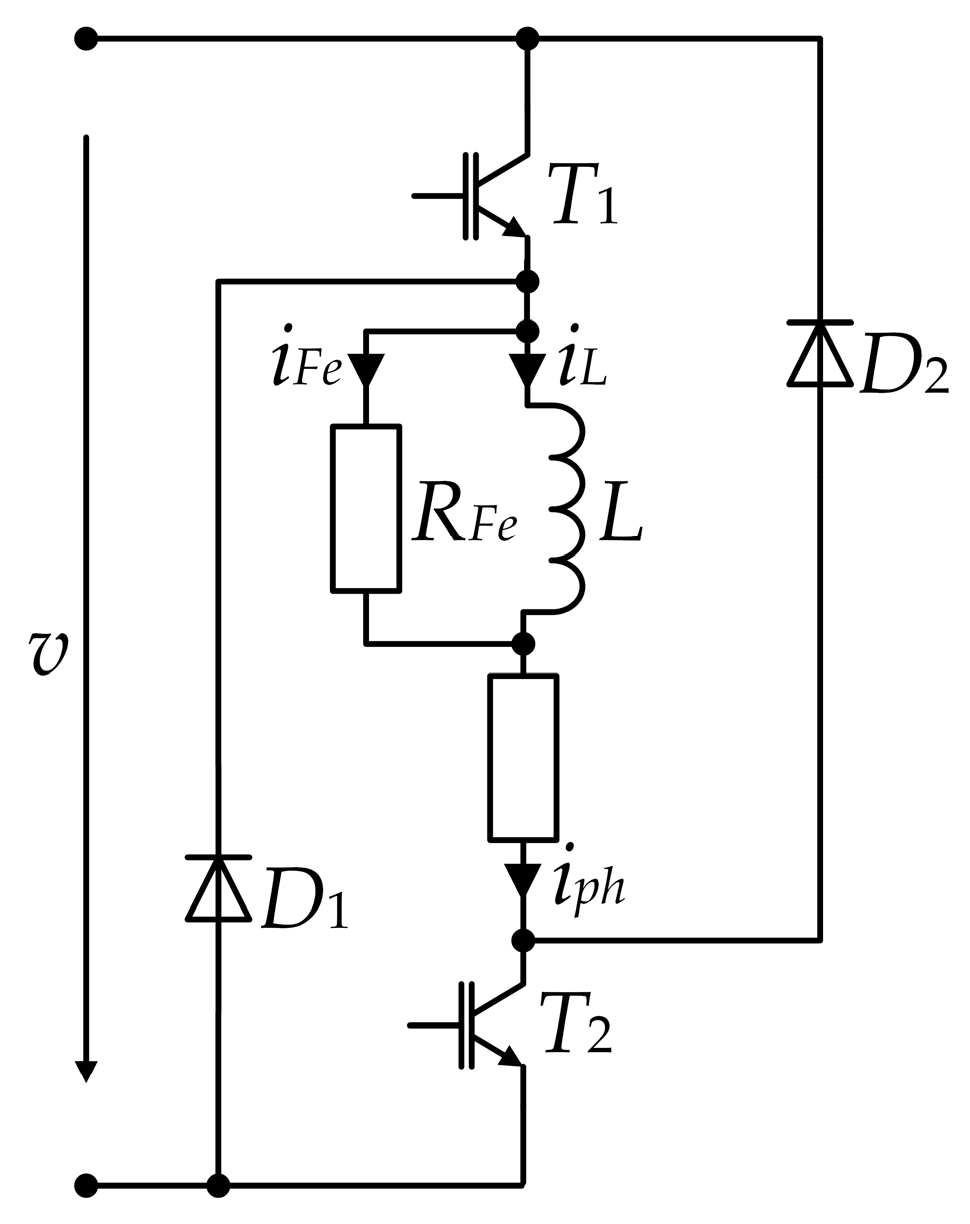
For an SRG to function, a power electronic converter is required. Numerous types of converters have been studied in the literature. The most common type of converter is the asymmetric bridge converter, as shown in
Figure 2, with the four-phase SRG, the load resistance
Rl, and the capacitor
C, which has the task of supplying energy for the phase magnetization. In this configuration, each phase of the SRG can be controlled separately, which ensures tolerance to phase fault.
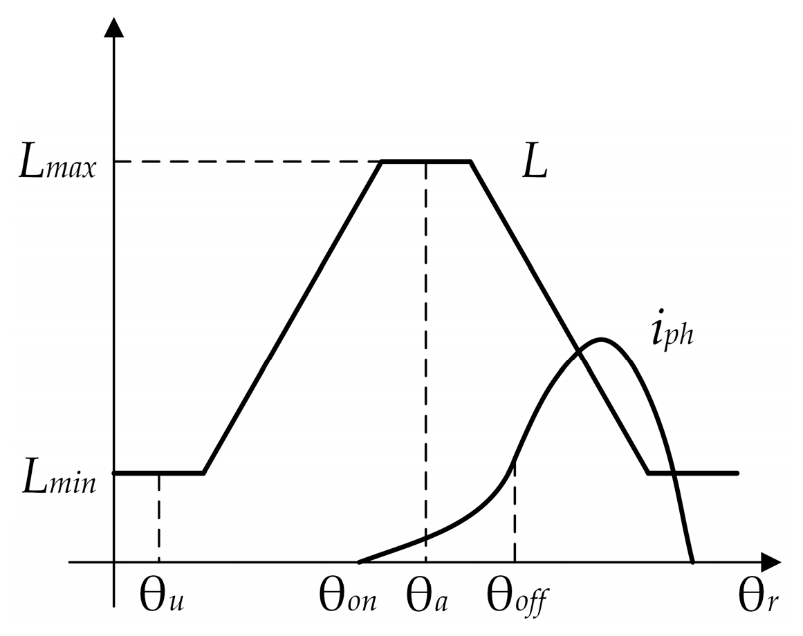
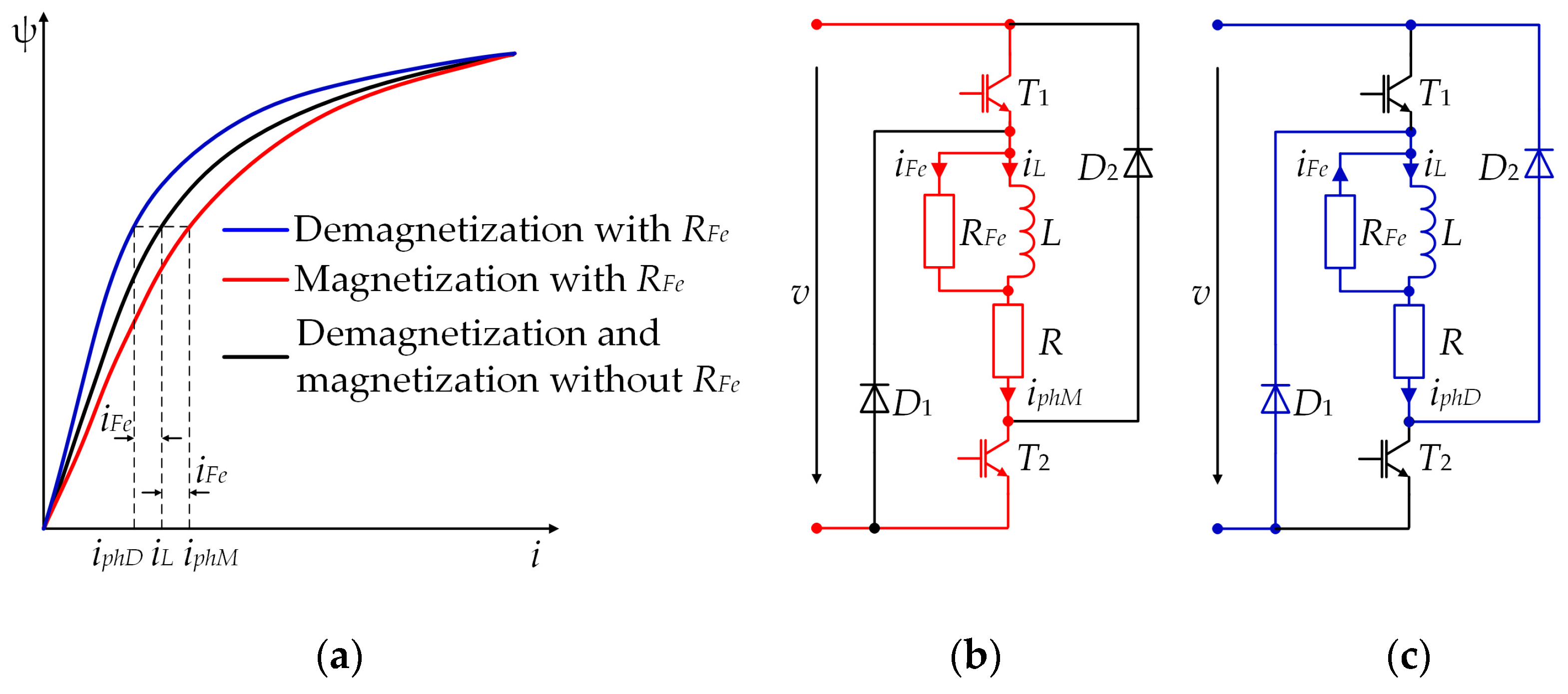
In this paper, two stages of SRG and converter are realized for each phase: magnetization and demagnetization (
Figure 3). The waveforms shown in
Figure 3 assume high-speed operation and linear analysis, which means that there is no magnetic saturation. Magnetization starts when the two transistors of the same converter leg are switched on (angle θ
on). During the magnetization of an SRG phase, the terminal voltage is applied to the magnetized phase and the phase current increases. The magnetization is completed at the time corresponding to the rotor position θ
off shown in
Figure 3 when the transistors are switched off. At this rotor position, the diodes in the same leg start to conduct the phase current and the phase inductance decreases, as shown in
Figure 3.
In addition to magnetization and demagnetization, there is a third state, which was first proposed by [
32] and is referred to as the freewheeling stage. In [
27], this stage is incorrectly referred to as “flux boosting” because during this stage the flux-linkage remains approximately constant. The third stage is observed when only one of the transistors of the same leg is switched on and the other is switched off (for example, the current of phase 1 in
Figure 1 flows through
T1 and
D2). The phase voltage is then zero. Applying the zero voltage to the phase reduces the current ripple of the terminal voltage. However, the output power is reduced [
33]. Therefore, the third state was not used in this paper.
The phase current waveform shown in
Figure 3 applies to high-speed operation, where the EMF is greater than the terminal voltage. This EMF causes the phase current to continue to rise even after θ
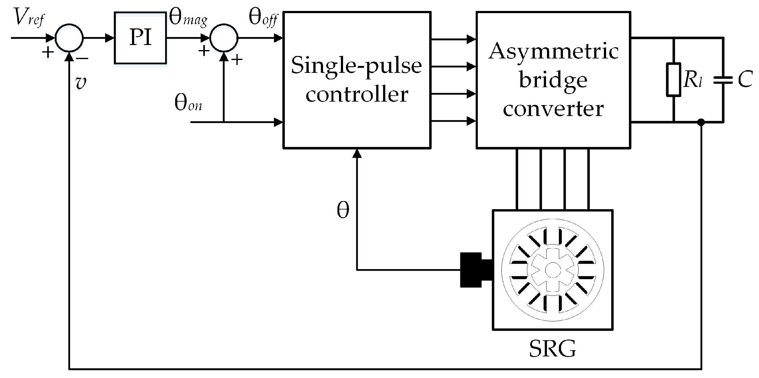
off, which can lead to a large uncontrolled phase current peak. One possible solution to avoid these peaks is the SRG terminal voltage control system shown in
Figure 4. As in [
34,
35], the terminal voltage is also the controlled variable in this paper. In [
34,
35], the output of the PI controller is turn-off angle, but instead of this angle, the magnetization angle is used in this paper. Considering that there is an analytical expression for the turn-off angle and the magnetization angle when the turn-on angle is fixed, it is ultimately irrelevant which of these two angles is used as the output of the PI controller.
The single-pulse controller shown in
Figure 4 determines the times at which the transistors of the same leg are switched on and off. If the rotor position is between θ
on and θ
off, the two transistors of the same leg switch on, otherwise they switch off. The main purpose of the control system shown in
Figure 4 is to validate the advanced simulation model of the SRG.
3. Conventional Mathematical Model of the SRG and the Asymmetric Bridge Converter
This section describes the conventional 8/6 SRG model connected to the asymmetric bridge converter and loaded by
Rl. The parameters of the SRG can be found in
Appendix A. In this model, each phase of the SRG is represented as a series-connected phase inductance
L with the winding resistance
R.
Figure 1 shows the equivalent circuit of the four-phase SRG connected to the asymmetric bridge converter.
The diodes
D1 and
D2 and the IGBTs
T1 and
T2, which are shown in
Figure 2, are modeled as ideal switches. The diodes and the transistors conduct alternately. When the transistors are switched on, phase magnetization begins, and when the transistors are switched off, the diodes conduct, and this process represents demagnetization. Therefore, and according to
Figure 2, the following equation applies to one phase of the SRG:
where
k denotes the switching state of the transistors;
v denotes the terminal voltage;
iph denotes the phase current;
R denotes the phase resistance; ψ denotes the flux-linkage; θ denotes the rotor position.
Equation (1) can be written in the following form:
where ω (=
dθ/
dt) denotes the rotor angular speed.
The phase current can be derived from (2) and expressed as follows:
When the transistors are switched on,
iph(0) = 0. Based on (3), the phase currents in all four phases of the machine are as follows:
where
j (
j = 1, …, 4) is the number of the phase.
The phase currents described by (4) are always positive. The terminal current shown in
Figure 1 is
The terminal current
i0 is divided into the current
iC, which flows through the capacitor
C, and the current
il, which flows through the load
Rl. The current
iC is therefore
The terms ∂ψ/∂
iph and ∂ψ/∂θ in (3) are still missing for a complete definition of the conventional mathematical model. Authors in [
26,
28] replace the flux-linkage in (3) as the product of the phase inductance and the phase current. Since the phase inductance changes periodically with the rotor position θ, it can be expressed as a Fourier series of the rotor position θ, which has current-dependent coefficients. Similarly, the Fourier series of the flux-linkage is expressed as a power series of the rotor position
where
Nr is the number of rotor poles.
The coefficients
Cl (
l = 0, 1, 2) in (7) are defined by the following equation:
where ψ
a(
iph), ψ
u(
iph), and ψ
m(
iph) represent the flux-linkages in the aligned (θ = 0°), unaligned (θ = 180°/
Nr), and midway position of the rotor (θ = 180°/2
Nr), respectively.
The flux-linkages in (8) are approximated by polynomials [
33]
where
aal,
aml, and
au are the polynomial coefficients obtained by the curve fitting technique of the experimental data obtained by the DC excitation method [
13]. These coefficients are listed in
Appendix B.
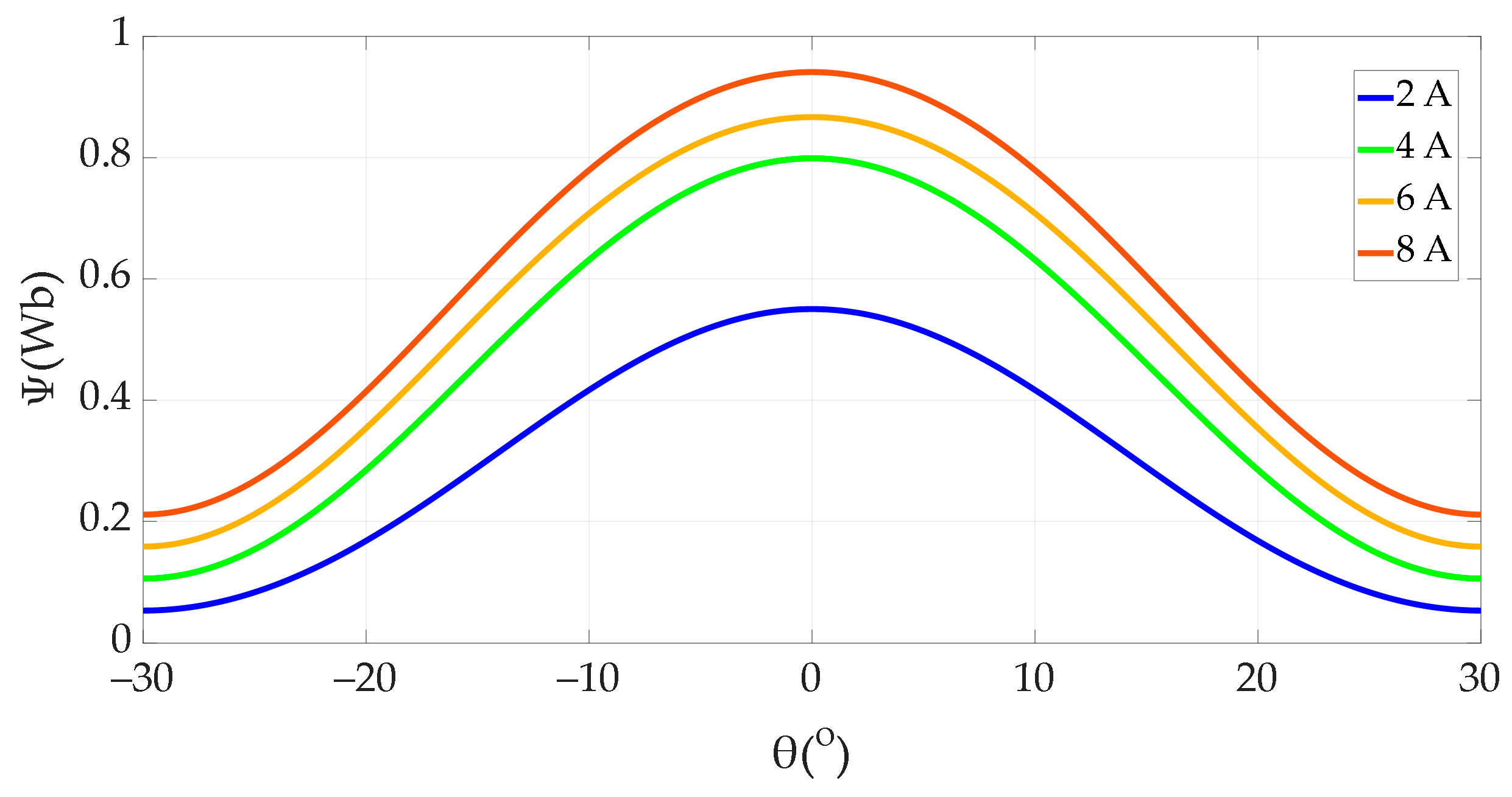
Substituting (8) and (9) into (7) gives
The term ∂ψ/∂θ, which is needed in (3), can be obtained from (7)
Substituting (10) and (11) into (3), the phase current
iph is completely determined. Using (7)–(9) and the polynomial coefficients given in
Appendix B, it is also possible to determine ψ(
iph,θ), as shown in
Figure 5.
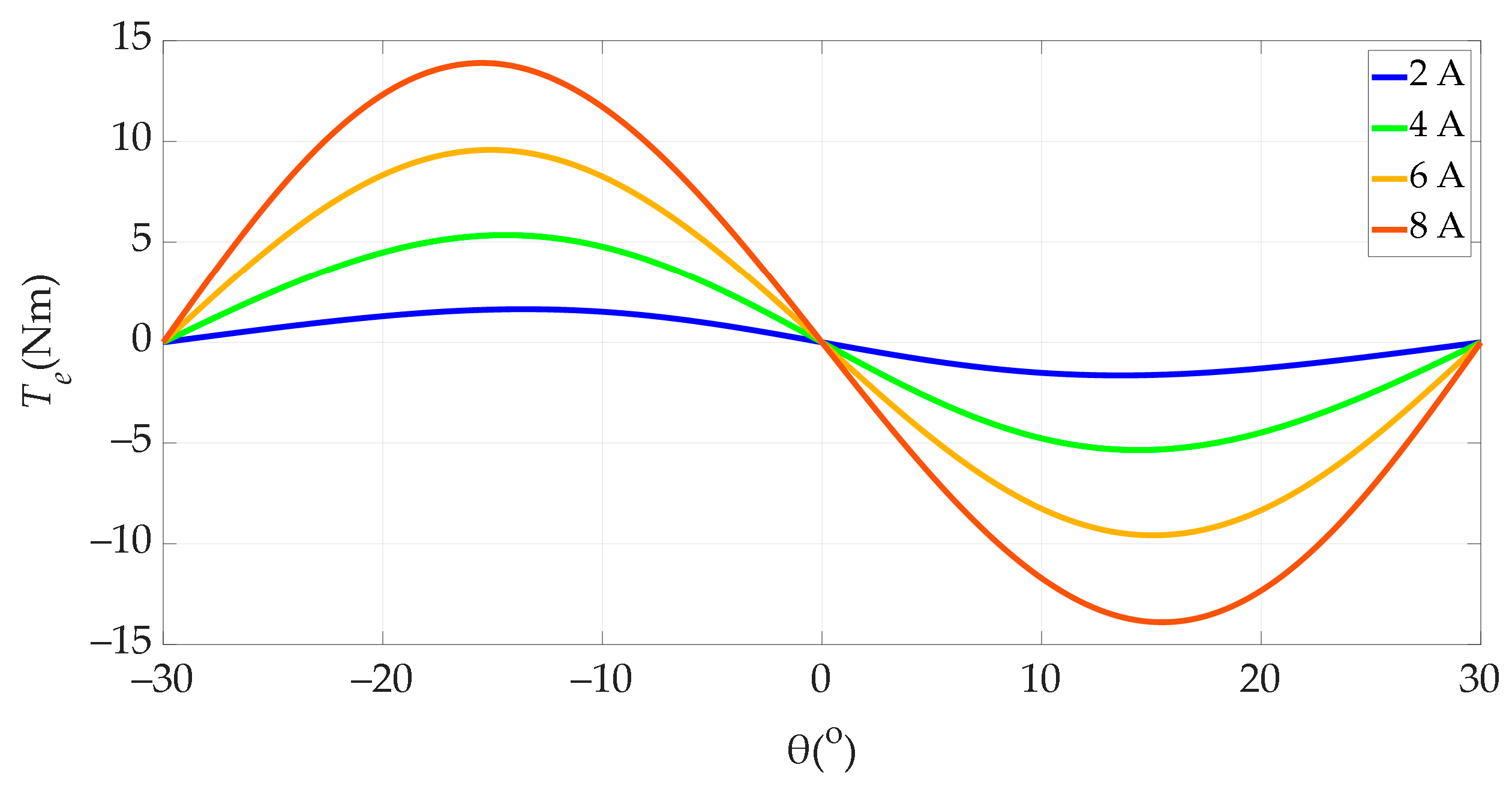
The electromagnetic torque of one phase is
where
Wc is the magnetic co-energy.
Using (7)–(9) and (12), the electromagnetic torque is defined as
Using the polynomial coefficients given in
Appendix A, the electromagnetic torque of a phase is obtained as shown in
Figure 6.
A positive electromagnetic torque corresponds to the motor operating mode and a negative one to the generator operating mode, as shown in
Figure 6.
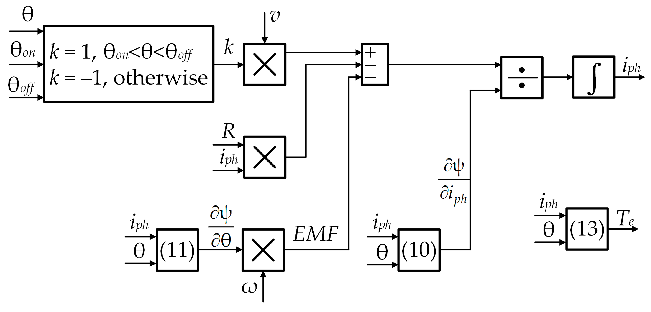
The full diagram of the conventional SRG model of one phase, which is basically a graphical representation of (3), is shown in
Figure 7.
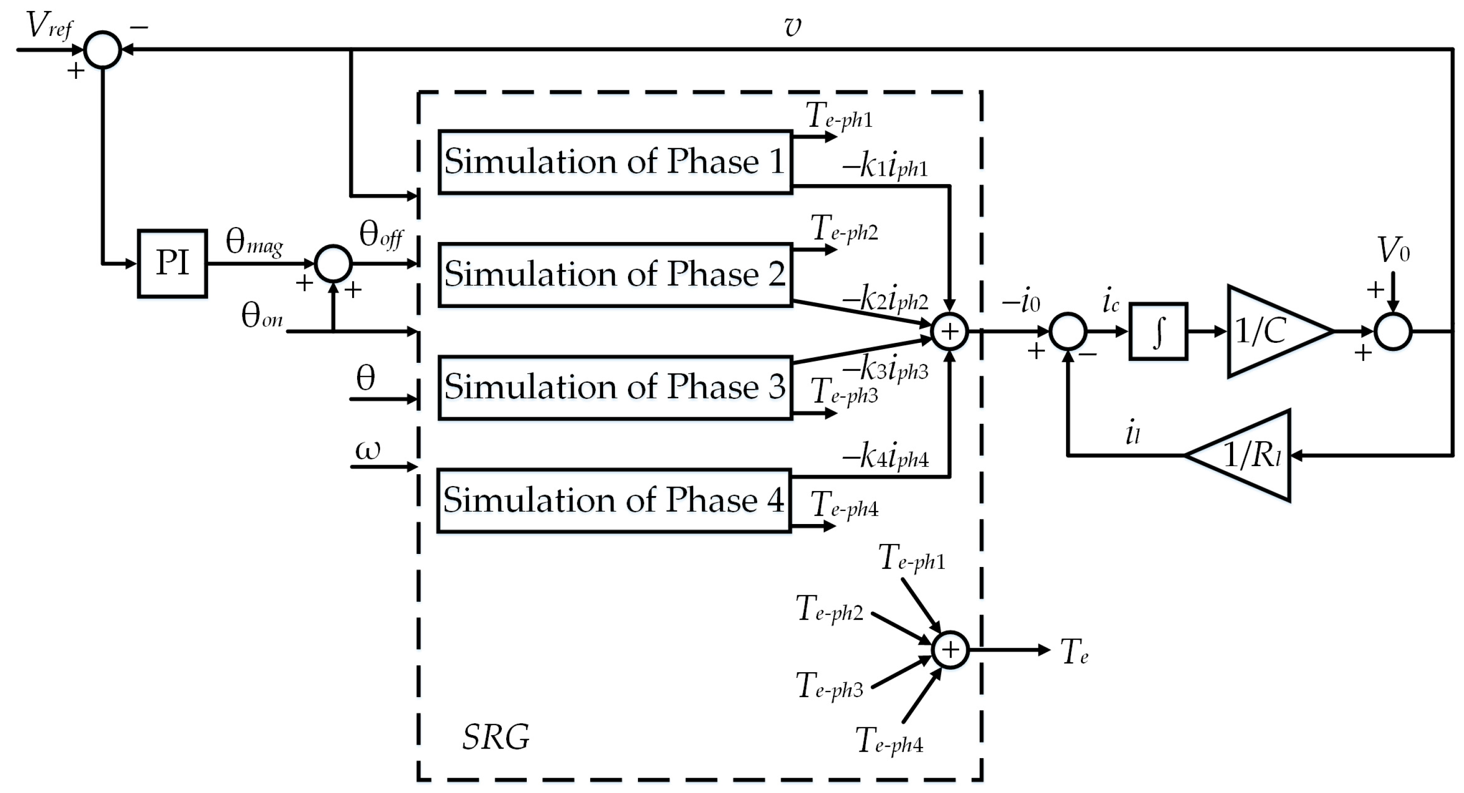
The diagram of the complete conventional SRG model together with the terminal voltage control system is shown in
Figure 8.
As shown in
Figure 8, the electromagnetic torque
Te and the terminal current
i0 are calculated based on the independent operation of the SRG phases.
The conventional SRG model does not take iron losses into account. This model provides symmetrical phase currents, and it was found in [
10] that the phase currents of SRG are not symmetrical. These facts are the reason for the development of the advanced model presented in
Section 4.
5. Experimental Validation of the Advanced SRG Model
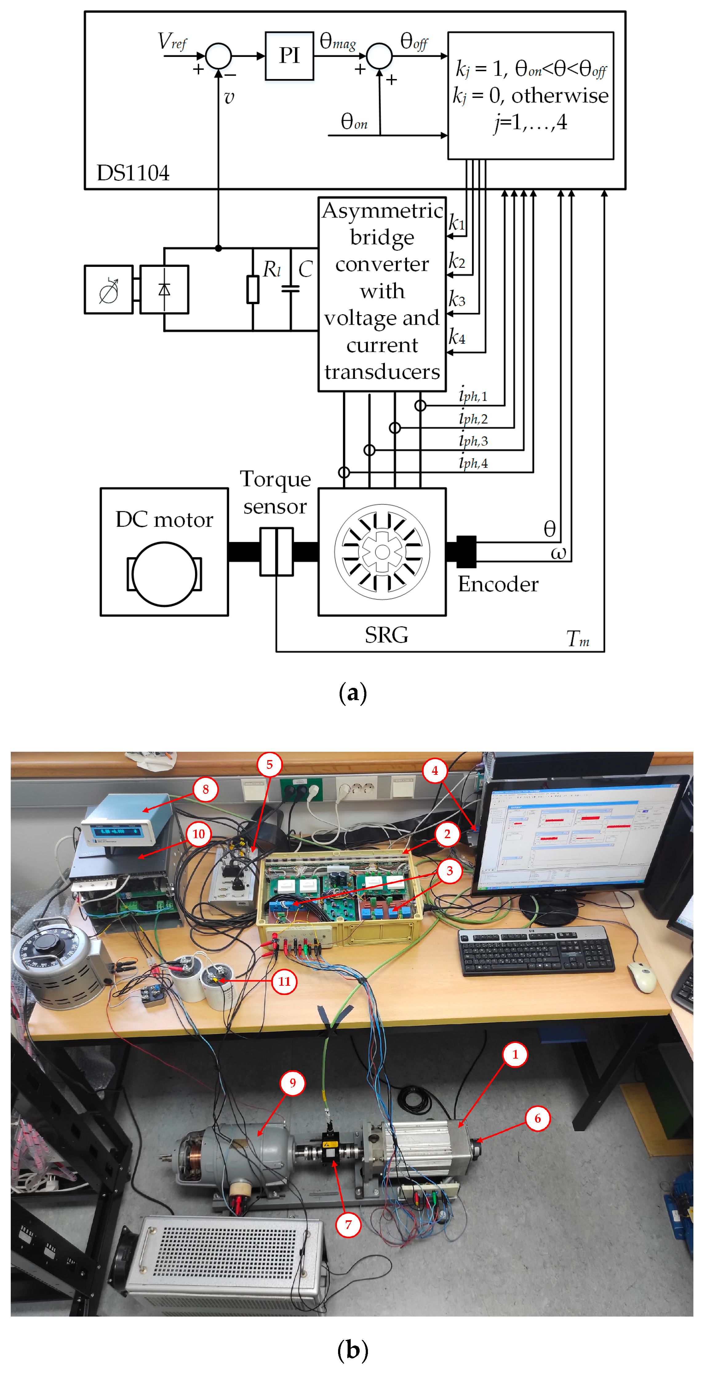
The experimental setup of the SRG control system used for the evaluation of the proposed advanced SRG model is shown in
Figure 21a, and the photo of the experimental setup is shown in
Figure 21b.
The names and data of the main components of the experimental setup shown in
Figure 21b are listed in
Table 1.
A series of experiments were conducted to determine the accuracy of the advanced SRG model. By combining rotor speeds of 2000 rpm and 3000 rpm, terminal voltages of 150 V, 200 V, 250 V, and 300 V, load resistances of 110 Ω, 65 Ω, and 45 Ω and turn-on angles of −15°, −10°, and −5°, 58 steady-state operating points were realized with the laboratory setup. The SRG was tested over a wide power range, from 18.6% to 126.6% of the rated power.
The DS1104 controller board was used for the real-time implementation of the control algorithm shown in
Figure 21 and for data acquisition. The control algorithm works reliably (i.e., without task overrun) up to a sampling frequency of 20 kHz, so this frequency was used. The parameters of the PI controller were determined by trial and error, using the integration gain
Ki = 5 and the proportional gain
Kp = 1.
For each operating point, the no-load torque was subtracted from the measured mechanical torque to obtain the electromagnetic torque Te generated by the SRG. To ensure the accuracy of the no-load torque measurement, the measurement was carried out in the range from 0 to 3000 rpm with an increment of 250 rpm and the measurement was repeated five times at each speed.
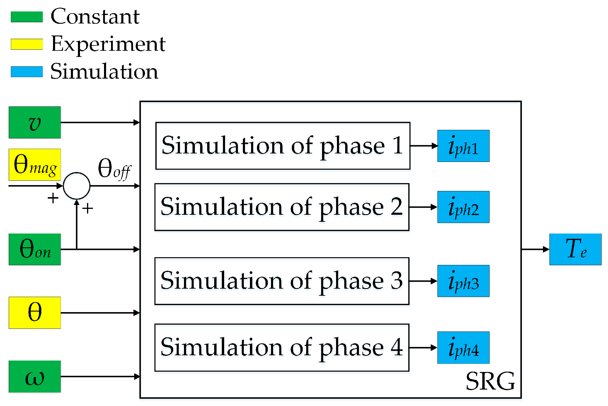
After conducting the experiments, simulations were carried out in Matlab/Simulink using the conventional and advanced model described in
Section 3 and
Section 4. The simulated phase currents and input powers were used for comparison with the corresponding measured values. The comparison is only possible if the simulations with the advanced and conventional model were carried out under the same conditions as the experiments. This means that the terminal voltage, the rotor speed, the turn-on and turn-off angles, and the rotor position must always be identical in the simulation and in the measurement. For this purpose, the so-called hybrid simulation model for steady-state conditions was developed, the diagram of which is shown in
Figure 22.
Note that the blocks labeled Simulation of phase 1, …, 4 in
Figure 22 may represent conventional or advanced simulation models of the SRG phases. The turn-on angle shown in
Figure 22 was selected as constant, as this angle was also constant in experiments. The terminal voltage
v was precisely controlled by the PI controller (
Figure 21) and considering a capacitor of 8800 μF, its ripple was less than 0.5% in experiments. Therefore, it is justified to consider the terminal voltage as constant, as shown in
Figure 22. The same applies to the rotor angular speed ω, which is controlled by the power converter.
In order to determine the accuracy of the conventional and advanced SRG simulation models, a simulation with a hybrid simulation model was also carried out for each of the 58 steady-state experimental operating points. The comparison of the experimentally determined phase currents with the phase currents obtained by the hybrid model, in which the phase currents were simulated by the advanced/conventional model, was carried out for a time of 4.75 s (95,000 samples) in the steady-state of the SRG. Each steady-state operating point of the SRG is completely defined by the load resistance
Rl, turn-on angle θ
on, the rotor speed
n (in rpm) and the terminal voltage
v. Therefore, the so-called accuracy coefficient is defined by the following equation:
where
iph,exp(
q) denotes the experimental value of the phase current at the
qth sampling instant and
iph,conv(
q)/
iph,adv(
q) denotes the phase current obtained with the conventional/advanced simulation model current at the
qth sampling instant.
According to (25), the advanced model is more accurate than the conventional model if K > 1. Otherwise, the conventional model is more accurate.
Figure 23 shows the phase currents and the magnetization angle for one of the 58 steady-state operating points defined by the following parameters:
Rl = 65 Ω, θ
on = –5°,
n = 2000 rpm and
v = 250 V. The simulated phase currents are determined using the hybrid steady-state simulation model, in which the phase current models are first based on the conventional model and then on the advanced model. The same figure also shows the experimentally determined phase currents in the control system shown in
Figure 21. According to
Figure 22, the magnetization angle is the same for all these phase currents and corresponds to the experiment.
In
Figure 23, it is easy to see that the phase currents obtained by the advanced simulation model of the SRG are in better agreement with the experimental phase currents. As already mentioned, the accuracy coefficient
K according to Equation (25) was chosen as a measure of this agreement. The accuracy coefficient for each phase of the SRG and for each of the 58 steady-state operating points is shown in
Figure 24.
Figure 24 shows a total number of 232 accuracy coefficients (58 × 4). The accuracy coefficient is greater than 1 in 226 cases, while it is less than 1 in 6 cases (points circled with a red line). This means that the phase current determined with the advanced simulation model is more accurate than that determined with the conventional model in 97.4% of cases. At the points where the accuracy coefficient is less than 1, in phases 2 and 3, it is possible in experiments that the remanent magnetic flux and the part of the flux-linkages of the neighboring phase cancel each other out. However, this cannot happen in the advanced model. In this case, the conventional model is more accurate than the advanced model, suggesting that discrete changes in remanent magnetic flux should be modeled more accurately. However, this modeling was not performed, as the number of such points is negligible.
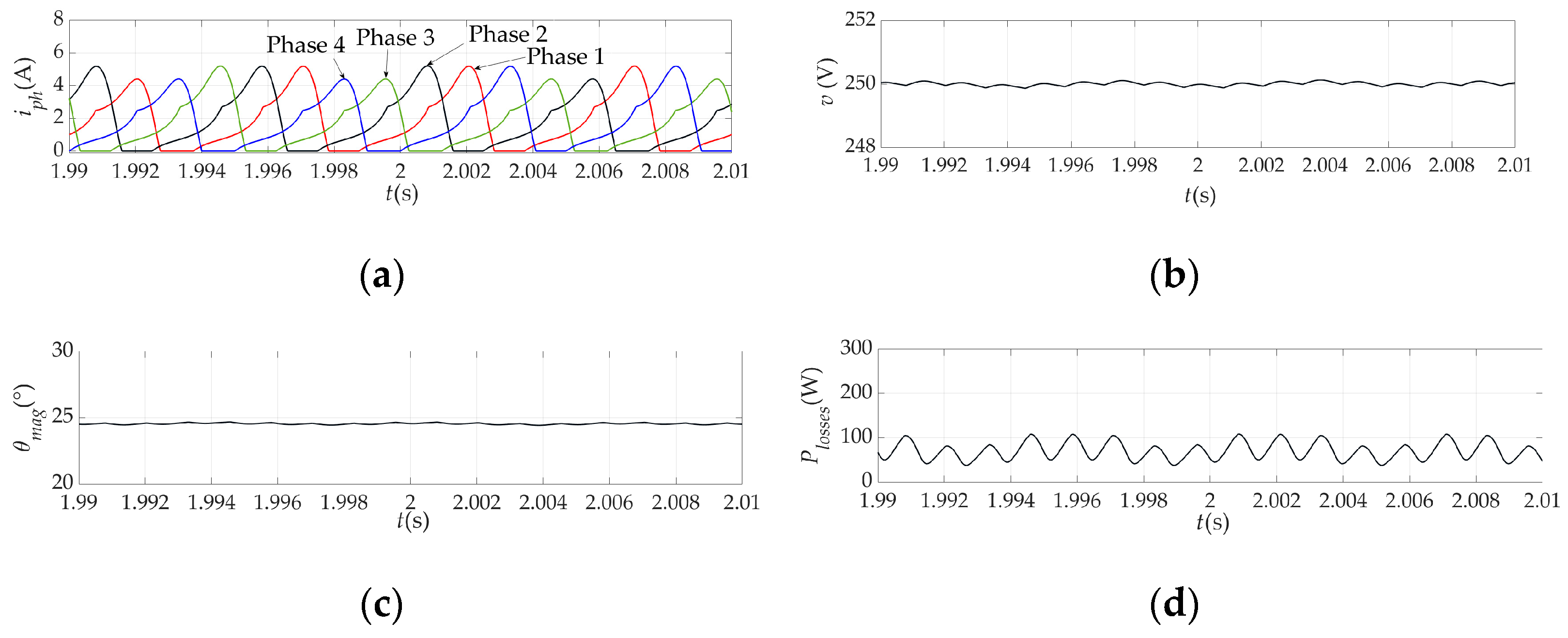
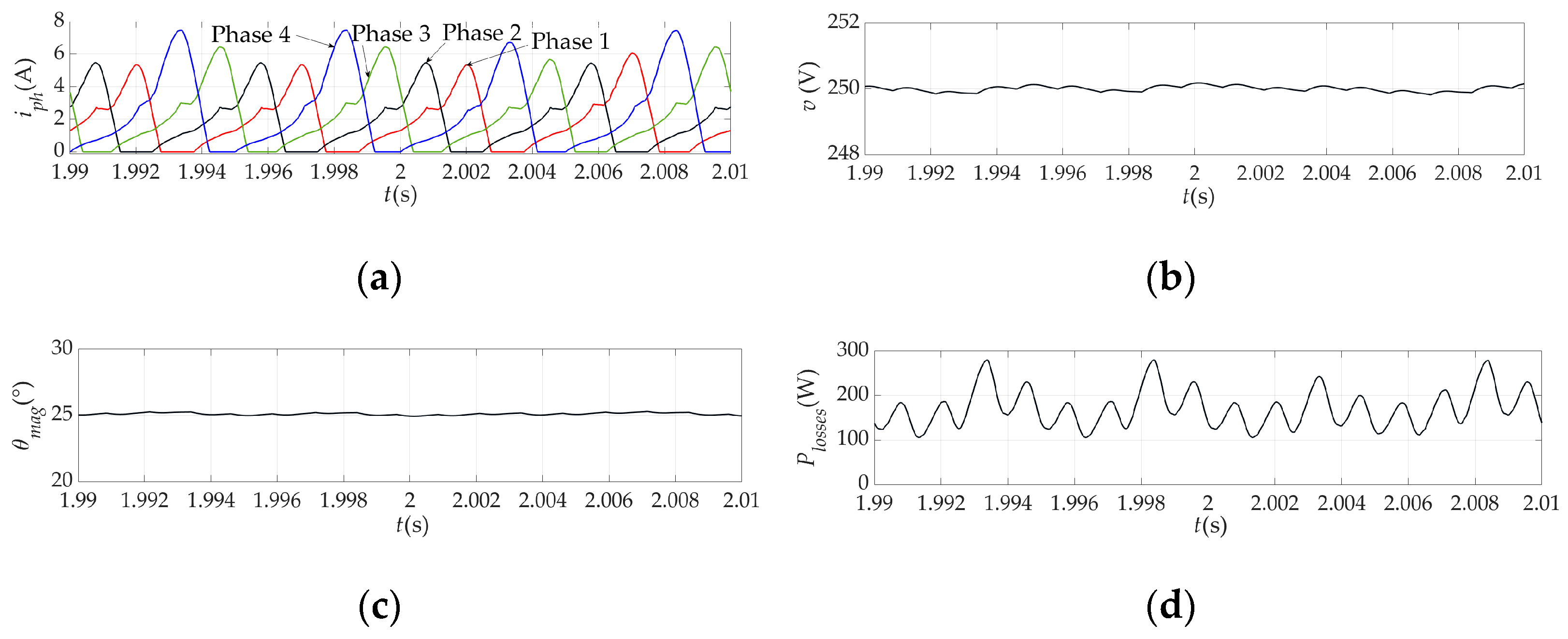
Finally, to show that the development of an improved SRG model is justified,
Figure 25 and
Figure 26 show the simulation results of the control system shown in
Figure 4, where the SRG model is conventional (
Figure 25) and advanced (
Figure 26). These figures show simulation results for the same steady-state operating point as in
Figure 21 (
Rl = 65 Ω, θ
on = −5°,
n = 2000 rpm and
v = 250 V).
Figure 25a and
Figure 26a show the SRG phase current determined using the conventional and advanced models, respectively. As expected, the peak values of the phase currents are higher when using the advanced model, as the iron losses are also taken into account. Therefore, the losses calculated with the conventional model (copper losses),
Figure 25d, are lower than the losses calculated with the advanced model (copper losses and iron losses,
Figure 26d). In the advanced simulation model, the current of phase 4 has a higher peak value than the other phase currents. This effect was also observed in the experiment (
Figure 23) and is due to the mutual coupling of phase 4 and its previously magnetized phase, i.e., phase 1. The flux-linkage of phase 1 is in the same direction as the flux-linkage of phase 4 and they support each other. As a result, the flux density of phase 4 is higher than that of the other phases and consequently the current of phase 4 is also higher.
The magnetization angle calculated with the advanced model (
Figure 26c) is higher than that calculated with the conventional model (
Figure 25c). There are physical reasons for this because in the SRG control system shown in
Figure 4, the magnetization angle increases with the load. In this case, the iron losses actually represent an additional load. Finally, the terminal voltage shown in
Figure 25b and
Figure 26b has a ripple of less than 0.7%, so that the terminal voltage is practically constant. A similar ripple occurs with the rotor speed.
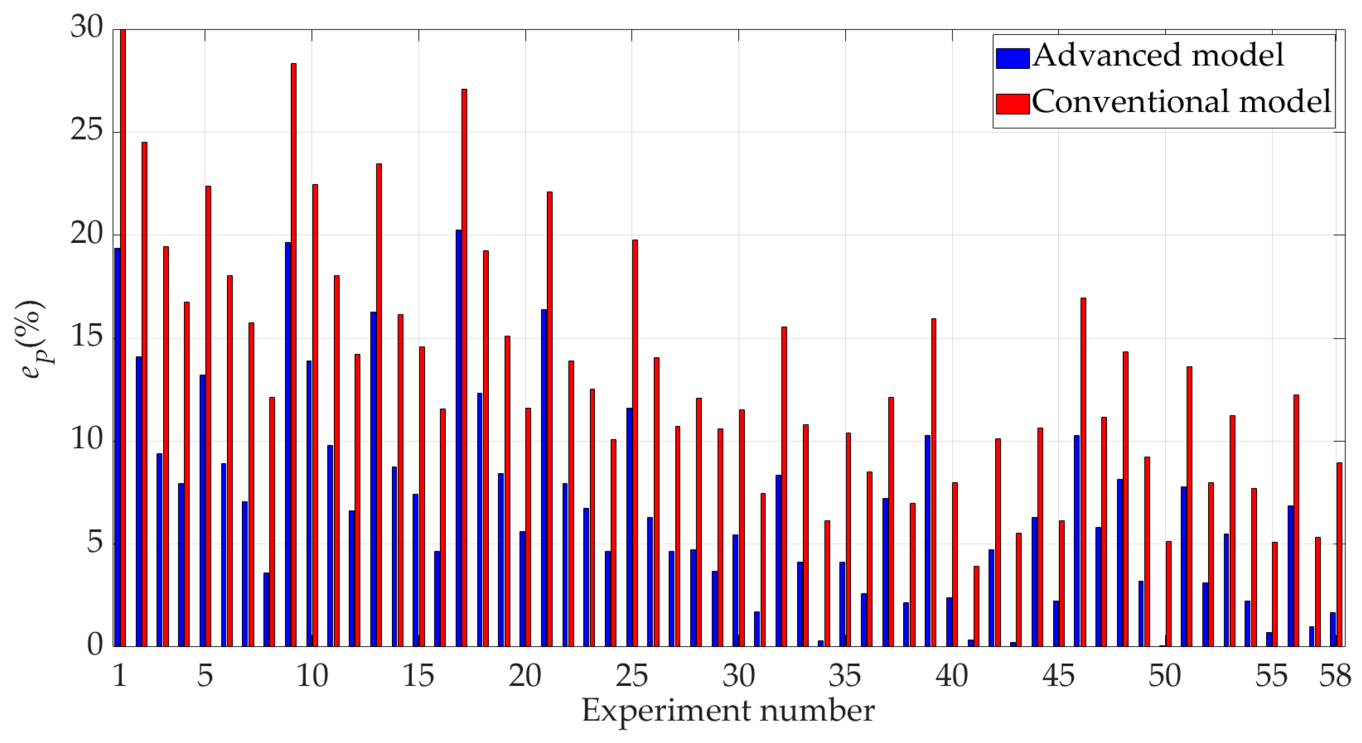
As a final step to check the accuracy of the simulation models, a comparison was made between the SRG input power calculated by the conventional and advanced simulation models and the experimentally determined input power for the same 58 steady-state operating points. The input power determined by the simulation was determined as the sum of the output power and the losses and not as the product of electromagnetic torque and power. This was performed because the electromagnetic torque is calculated according to (12), which implies a differentiation with respect to the rotor position and therefore contains a larger numerical error. It is important to emphasize again that the mechanical losses are not considered in the SRG model itself. These losses are subtracted from the measured mechanical torque to obtain the experimental electromagnetic torque, which is then multiplied by the rotor speed to obtain the input power Pin,exp.
The mechanical input power is measured by the torque transducer in the experiments. To compare the input powers, the relative difference
eP between the experimentally determined input power and the input power calculated with the simulation models is defined by the following equation:
where
eP denotes the relative difference between the experimentally determined input power and the input power determined by simulation,
Pin,exp denotes the experimentally determined input power, and
Pin,sim denotes the input power determined by simulation (conventional or advanced model).
Figure 27 shows the relative differences between the input power of the SRG determined by simulations and the experimental power for 58 steady-state operating points.
The mean relative difference between the experimentally determined input powers and the input powers calculated with the advanced model in
Figure 27 is 6.95%, and the mean relative difference between the experimentally determined input powers and the input powers calculated with the conventional model is 13.54%. It can also be seen that the advanced model is more accurate than the conventional model at all steady-state operating points. As the SRG output power increases, the accuracy of the advanced model also increases, so that it has the highest accuracy around the rated power and above the rated power of the SRG (points 3, 12, 16, 20, 24, 27, 30, 31, 34, 37, 38, 41, 44, 45, 47, 49, 50, 52, 54, 55, 57 in
Figure 27) when the relative difference of the advanced model is between 0.05% and 7.96%. Despite this fact, the error of the advanced model is not zero, which means that the advanced SRG model does not fully describe the real SRG. The reason for this is that neither the semiconductor losses nor the so-called stray losses of the SRG were modeled. However, based on the data sheet of the diodes and transistors used in the experiments, the semiconductor losses in the experiments were also calculated and it was found that they account for a maximum of 21.6% of the total losses of the SRG and as such were not included in the
Pin,sim calculation. On the other hand, the stray losses of the SRG were not considered as they do not account for more than 6% of the total losses of the SRG according to [
9]. In comparison, the copper losses calculated using the advanced SRG model based on 58 steady-state operating points account for up to 66% of the total losses in some cases, while in other cases the iron losses account for up to 44.7% of the total losses.
6. Conclusions
This paper presents a model of SRG that takes into account the effects of mutual coupling, iron losses, and remanent magnetism. It is shown that it is sufficient to consider only the mutual coupling between a considered phase and a previously magnetized phase to accurately capture the effect of mutual coupling. The iron losses were successfully modeled by taking the SRG phase current component responsible for these losses directly from the look-up table, which justifies the simplicity of the advanced SRG model. The effects of mutual coupling and remanent magnetism in the equivalent circuit of one phase are represented as the EMFs. All data required for the development of the advanced SRG model were obtained using the DC excitation method and no machine design data were required.
To evaluate the advanced SRG model, a laboratory setup was designed with an 8/6 SRG with a rated power of 1.1 kW connected to the asymmetric bridge converter. The terminal voltage was controlled. The simulation results obtained with both the advanced and conventional models in single-pulse operation were compared with the experimental results obtained in steady-state over a wide range of loads, terminal voltages, duty angles and rotor speeds. It was found that the SRG phase currents simulated with the advanced SRG model matched the experimental results better than the SRG phase currents simulated with the conventional SRG model in 97.4% of the steady-state conditions considered. This is the main advantage of the advanced SRG model compared to the conventional one. If the semiconductor losses of the asymmetric bridge converter are taken into account in the simulation analysis, an even better match between the input power obtained by the advanced model and the experimentally determined input power would be achieved.
The proposed model is not suitable for the simulation of SRG failure states, since, for example, if one of the SRG phases is interrupted, the mutual couplings between the phases are different from those in normal operating mode.
The advanced SRG model was experimentally tested in SRG single-pulse mode, but it is also applicable in PWM current control mode and motoring mode. A more precise determination of the remanent magnetic flux as a function of the position of the rotor and the phase current of the SRG opens up the possibility of improving the proposed model. Moreover, this model is not limited to the SRG control strategy; it can also be applied to other voltage or power control strategies. All this is a topic for future research.


