Abstract
Electromagnetic field analysis and loss calculation is crucial for designing and optimizing magnetic components in high-frequency applications. The traditional method of combining eddy current field equations with hysteresis models is often used for low-frequency conditions and has complex applications due to the large number of coefficients. The loss calculation of commercial finite element software is usually in the post-processing phase, making the loss calculation and electromagnetic field analysis irrelevant. In this article, a new two-dimensional electromagnetic field analysis and loss calculation method for high-frequency applications is proposed based on vector magnetic circuit theory. The effects of eddy currents and hysteresis on the magnetic field can be considered simultaneously, and the corresponding eddy current losses and hysteresis losses can also be directly calculated. Two toroidal magnetic cores for high-frequency applications are used to verify the effectiveness and accuracy of the method proposed in this article. The analytical calculation results have higher accuracy compared to the ANSYS simulation results.
1. Introduction
The emergence of wide-bandgap (WBG) semiconductors has revolutionized power electronic systems by enabling high-frequency operation in converters and motor drives. This further reduces the size of passive components (inductors and capacitors) in power electronics. However, none of the soft magnetic materials available today are able to unlock the full potential of WBG-based devices [1]. The bottleneck now lies in magnetic components, with magnetic components accounting for more than 30% of the cost and more than 30% of the loss in almost all power converters [2]. With the development trend of high efficiency and high power density, magnetic component design has become a critical issue for power electronics [3]. Deep understanding and accurate design tools are required in magnetic components to comply with the trend toward high frequency and high power density [4].
The two most concerned performances of magnetic materials in power electronics applications are permeability and core loss, both of which vary significantly with frequency and the strength of the magnetic field (excitation signal) applied [3]. Currently, there are three main methods for calculating the core loss, such as the Steinmetz equation method (SE), loss separation model, the Preisach model and Jiles–Atherton (J-A) model [5,6,7,8]. These methods to account for the core loss and permeability, mostly empirical, are extracted by curve fitting the experimental results measured from specific prototypes [9]. The problem is that empirical parameters cannot reflect the high-frequency effects of magnetic materials, as well as the distribution of magnetic flux and losses, which is crucial for the optimization and thermal management of magnetics [10].
Loss calculation is only a part of magnetics design and optimization. The modeling and electromagnetic field analysis of magnetics also need to be considered. Combining the hysteresis model and loss separation model, some scholars analyze electromagnetic systems with hysteresis and eddy current effects by introducing equivalent reluctivity or equivalent magnetic field strength into the two dimensional (2-D) electromagnetic field calculation equation [11,12,13,14,15]. This equivalence will make the convergence of the model unstable [16]. Moreover, these models still need to include a large number of parameters required for hysteresis models, which brings inconvenience to practical applications. There is another vector hysteresis model, the E&S model, proposed by M. Enokizono and N. Soda to consider the rotational and alternating losses of the magnetic core [17,18]. This model considers the effect of hysteresis on the magnetic field by introducing an effective hysteresis coefficient, which is worth referencing. However, the E&S model has the problem of repeated consideration of eddy current effects because the magnitude of the hysteresis coefficient of the E&S model is related to both eddy current loss and hysteresis loss [19].
The methods mentioned above are mainly applied to silicon steel sheets. However, for magnetics, such as ferrites, used in high-frequency applications, commercial finite element software is still the preferred choice for researchers and engineers [5,20,21]. In commercial finite element software, such as ANSYS, it is necessary to first perform electromagnetic field calculations on the solution domain and then calculate the core losses using the relationship curve between B and power loss P (B-P curve), the SE, loss separation model, or other models in the post-processing process [22,23]. There are three problems with this approach: (1) The accuracy of core loss calculation heavily depends on the parameters of the loss model. (2) It remains unclear whether commercial FEM software inherently accounts for hysteresis and eddy current reactions in the magnetic field. (3) The calculated losses may not accurately reflect their actual impact on the magnetic field due to the reliance on empirical coefficients.
Considering the limited application of hysteresis models for high frequencies and the problems with commercial finite element software, this paper proposes a new two-dimensional electromagnetic field analysis and loss calculation method for high-frequency applications based on the vector magnetic circuit theory [24,25,26]. Different from the traditional scalar magnetic circuit with only reluctance, the vector magnetic circuit includes three components, i.e., reluctance, magductance, and hysteretance. This method characterizes the hysteresis and eddy current effects by hysteretance and magductance, respectively; thus, the analytical eddy current loss and hysteresis loss models are developed. This paper combines the vector magnetic circuit theory with two-dimensional electromagnetic field analysis and loss calculation so that the effects of hysteresis and eddy currents on the magnetic field can be considered separately. The corresponding loss values can be simultaneously calculated instead of using loss coefficients in post-processing.
In this article, the vector magnetic circuit theory is briefly recalled in Section 2, and the new method is introduced in detail in Section 3. The required parameters and application of the proposed method are described in Section 4. By analyzing and calculating two toroidal ferrite cores, the analytical calculation results are compared with ANSYS simulation and experimental data in Section 5, verifying the accuracy and effectiveness of the method. The conclusion of this article is summarized in Section 6.
2. Introduction to Vector Magnetic Circuit Theory
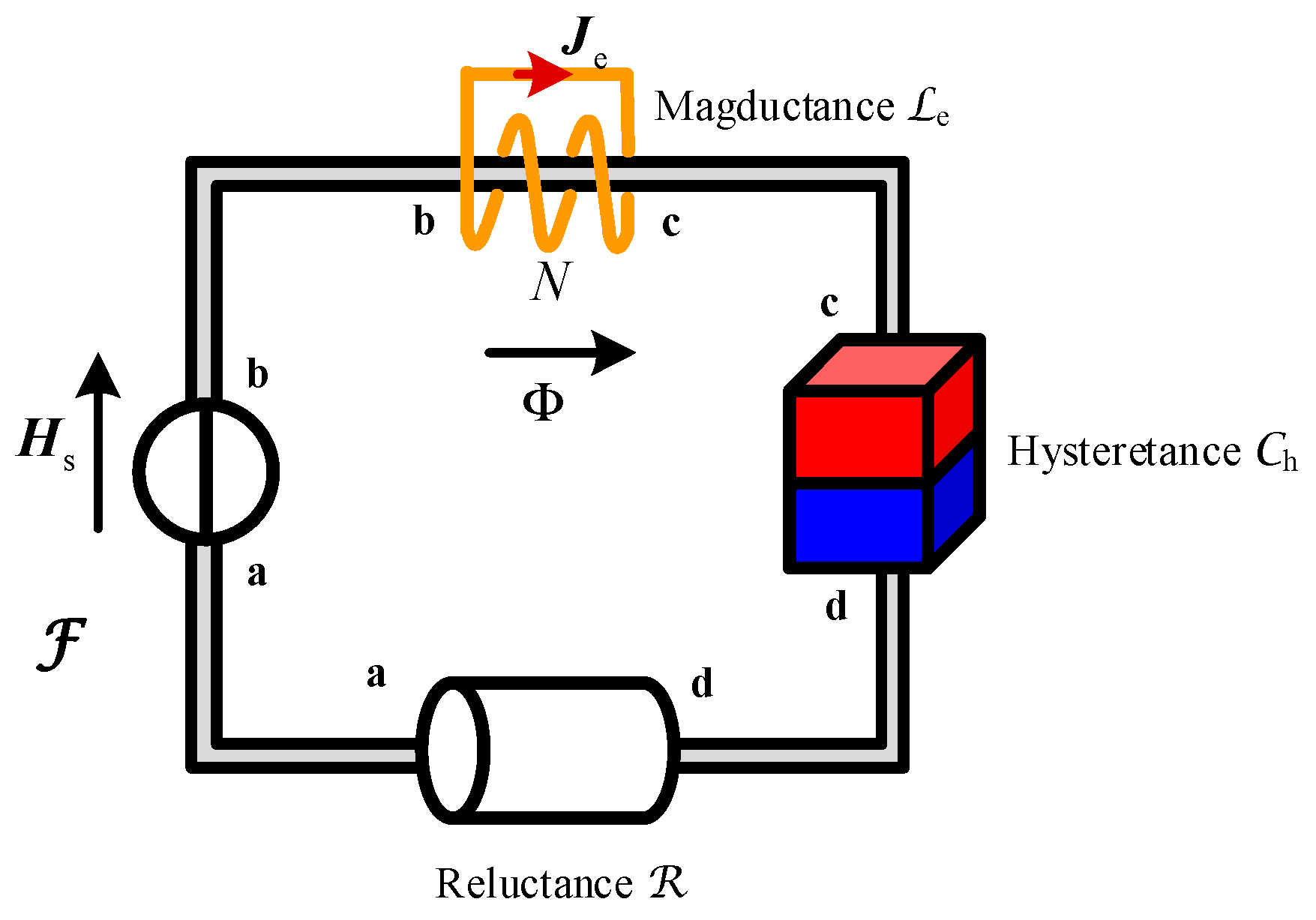
According to vector magnetic circuit theory [24,25], a vector magnetic circuit can be represented as shown in Figure 1, with the assumption that the magductance of the entire magnetic circuit is concentrated on the magductance component in the bc segment, the hysteretance Ch of the entire magnetic circuit is concentrated on the hysteretance component in the cd segment, and the reluctance of the entire magnetic circuit is concentrated on the reluctance component in the da segment. Hs is the magnetic field strength generated by source current. Je is the current density on the magductance component. is the magnetomotive force (MMF). Φ is the magnetic flux. N is the number of turns of the magductance component.
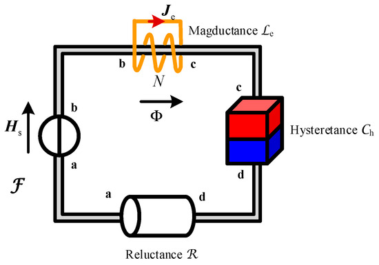
Figure 1.
Vector magnetic circuit.
The magnetic circuit shown in Figure 1 satisfies the following basic relationship:
where,
are the MMF on the reluctance, magductance, and hysteretance components, respectively.
(1) MMF source: The left integral of (1) is equal to the MMF generated by the excitation source:
where l is the length of the magnetic circuit.
(2) Reluctance effect: The first term on the right side of (1) represents the MMF drop on the reluctance component, so the port characteristics of the reluctance can be expressed as:
where S are the cross-sectional area; μ is the magnetic permeability.
(3) Magductance effect: The second term on the right side of (1) represents the MMF generated by the closed conductive coil, which can be expressed by a new magnetic component of magductance as:
where He is the vector potential generated by eddy currents. Because the eddy current in magnetic core can be equivalently modelled by a closed conductive coil, the magductance can characterize the eddy current effect of the magnetic core.
(4) Hysteretance effect: The third term on the right side of (1) represents the MMF generated by the hysteresis effect of the magnetic core, which can be expressed by a new magnetic component of hysteretance. Therefore, the port characteristics of the hysteretance can be expressed as:
where φm is a scalar magnetic potential related to hysteretance.
Combining (1)–(5), it can be concluded that:
The calculation equations for
for specific magnetic cores are as follows [25,26]:
where R represents the resistance of the magductance component or closed conductive coil; γ is the hysteresis angle.
3. New Two-Dimensional Electromagnetic Field Analysis and Loss Calculation Method
When the relative magnetic permeability of the material satisfies the condition μr >> 1, magnetic flux leakage can be ignored, and it can be assumed that the magnetic flux passes completely through the magnetic circuit, as shown in Figure 1. According to (1)–(8), the relationship between B and H can be obtained:
When the permittivity ε and conductivity σ of the material satisfy the condition σ >> ωε, the displacement current is negligible. Based on Maxwell’s equation and introducing vector magnetic potential A, the following expression can be obtained by simultaneously taking the curl on both sides of (9). The permeability in the solution domain is assumed to be constant, and gradient terms of permeability are neglected.
Here, , and .
For isotropic materials, without considering the anisotropy of magnetic permeability in the x and y directions, the two-dimensional electromagnetic field represented by vector magnetic potential A and current density J is:
According to (11), after considering the hindering effect of He on Hs, the amplitude and angle relationship between B and H can be obtained as the following two-dimensional expressions:
Under sinusoidal steady-state excitation, (11)–(13) can be changed to:
The eddy current loss Pe (W) and hysteresis loss Ph (W) of the magnetic core can be, respectively, calculated as:
where V represents the volume of magnetic core. Equations (11)–(13) are the general form of the new method of electromagnetic field analysis proposed in this paper, and (14)–(18) are the application form of this new method under sinusoidal steady-state excitation. Equations (11) and (14) can be transformed into variational forms or weak forms and then discretized and solved to handle the electromagnetic field computation of complex structures.
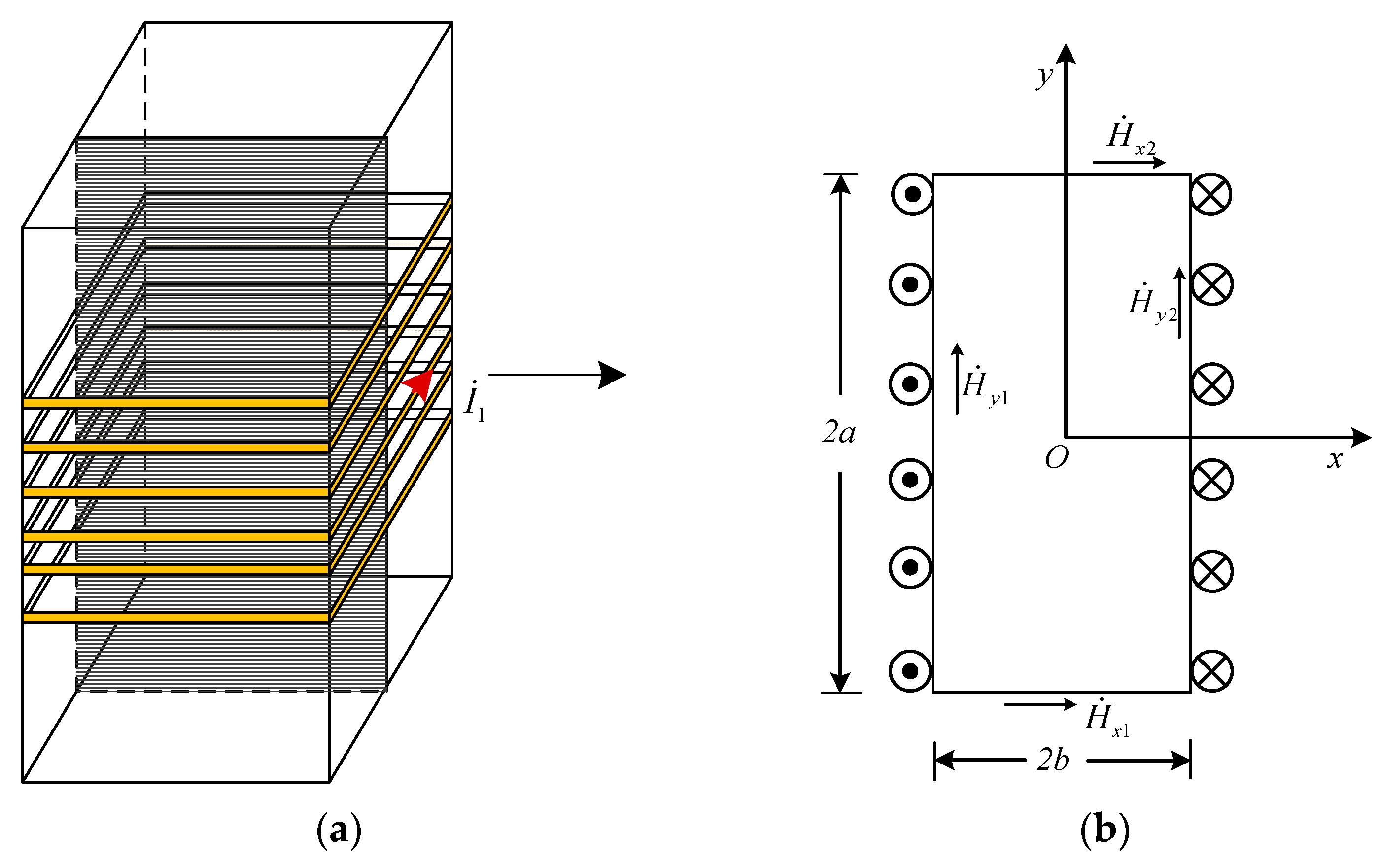
For the simple and direct verification of the rationality of the proposed method, an analytical expression of the two-dimensional rectangular cross-section is derived in this paper. Taking a magnetic core used in a transformer as an example, the magnetic core is located in the magnetic field generated by the primary coil, as shown in Figure 2a, where the arrow represents the direction of excitation current in the coil. Assuming that the coils are tightly attached to the surface of the magnetic core and the magnetic field generated by the coils is approximated as a two-dimensional magnetic field in a plane, as shown in Figure 2b, the problem can be simplified as a two-dimensional sinusoidal electromagnetic field problem.
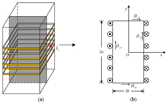
Figure 2.
Rectangular magnetic core in two-dimensional sinusoidal magnetic field. (a) Magnetic core wrapped by winding. (b) Two-dimensional model of shaded cross-section in (a).
As shown in Figure 2a, ideally, the current in the coils will only generate an MMF along the z direction, which will generate eddy currents and vector magnetic potential along the z direction in the xOy plane. In the eddy current region shown in Figure 2b, under sinusoidal steady-state conditions, satisfies the two-dimensional complex electromagnetic field equation:
The boundary conditions for the magnetic core are:
Assuming that the solution of (19) consists of and parts, and , respectively, satisfy the following boundary conditions:
Based on (21), can be decomposed into:
According to Figure 2b, the origin of the coordinate system is located at the center of the cross-section, and the cross-section is symmetrical about both the -x and y-axes. Therefore, the cos function is used as the solving function [27], assuming the solutions of and are:
The magnetic flux density inside the magnetic core is:
By combining (15), (16), (24), and boundary conditions (21), the undetermined coefficients can be solved as:
The current density inside the magnetic core is:
The eddy current losses of the core can be obtained by combining (17) and (27), and the hysteresis loss of the core can be obtained by combining (15), (16), (18), and (24).
4. Acquisition and Application of Required Parameters
4.1. Characteristics of the Magnetic Cores
For specific ferrite cores, material manufacturers usually only provide some general parameters of magnetic cores, such as the size, magnetic permeability, conductivity, and core-loss-per-unit-volume curves at some excitation frequencies and temperatures under sinusoidal excitation without dc bias [28,29]. The specifications of the magnetic cores studied in this article are listed in Table 1.

Table 1.
Specifications of magnetic cores.
The three-dimensional model of the magnetic core is shown in Figure 3.
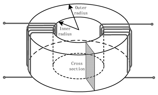
Figure 3.
The three-dimensional model of the magnetic cores 3E6 and N87.
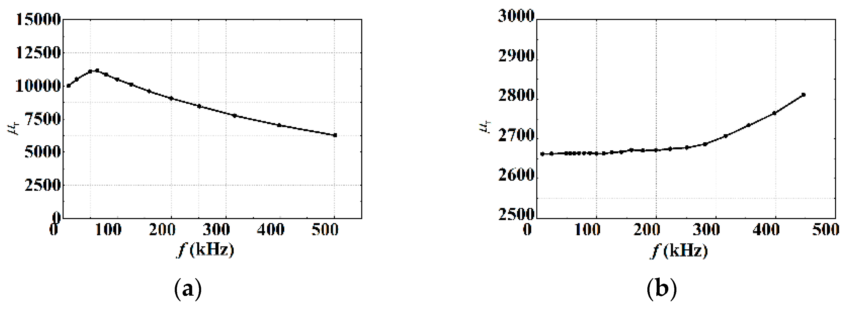
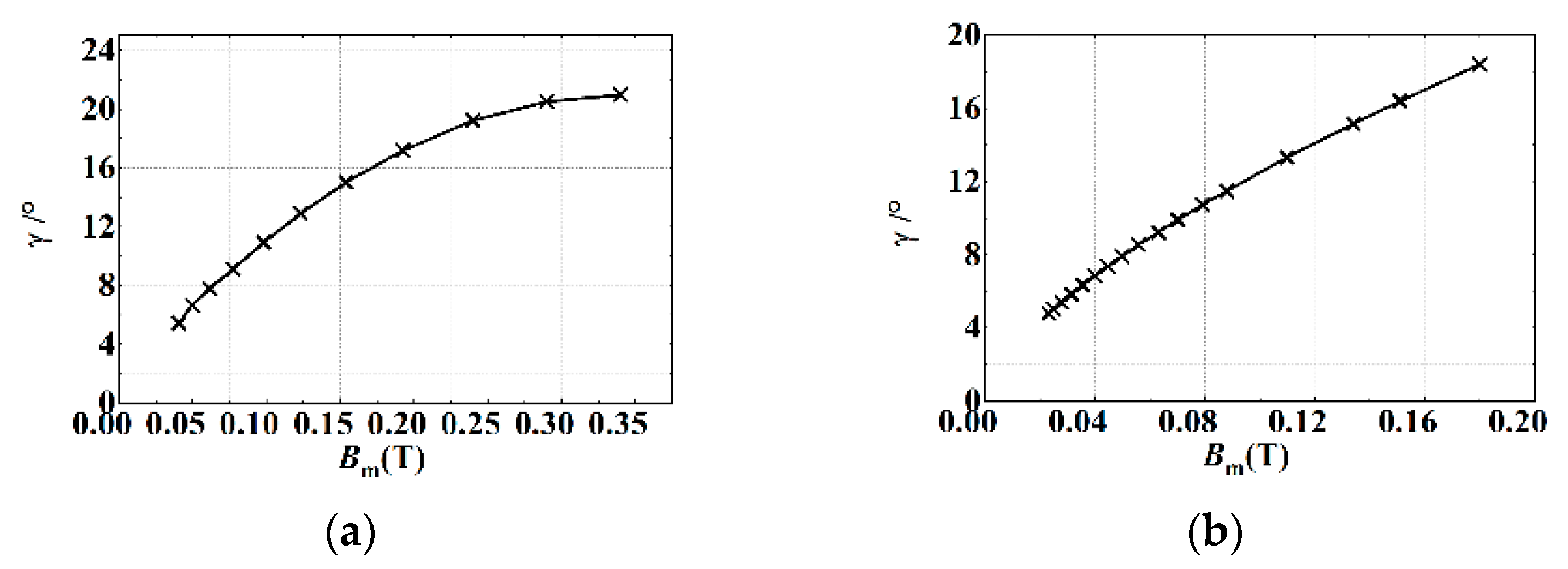
According to (12), the calculation of Ch requires the values of magnetic permeability μ and hysteresis angle γ. The curve of relative permeability μr with frequency f variation is shown in Figure 4 and is usually provided by the material manufacturers. However, γ is usually not provided by the material manufacturers. Hence, the relationship between the hysteresis angle and magnetic flux density under quasi-static condition of 3E6 and N87 magnetic cores is measured using the method in [25] and is shown in Figure 5.
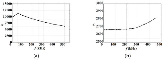
Figure 4.
The value of magnetic permeability μ with frequency of magnetic cores 3E6 and N87. (a) 3E6. (b) N87.
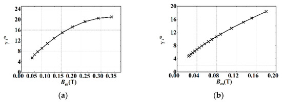
Figure 5.
The variation of hysteresis angle γ with frequency and magnetic flux density under quasi-static condition of magnetic cores 3E6 and N87. (a) 3E6. (b) N87.
From Figure 5, it can be observed that the hysteresis angle γ undergoes nonlinear change with the magnetic flux density. Figure 5 can serve as a material characteristic of the 3E6 and N87 magnetic cores introduced in this article. In practical calculations, specific values can be obtained by directly reading the table or fitting the curve. Additionally, the conductivity is considered to be a fixed value in this article.
Neglecting flux leakage, the boundary conditions are determined according to Ampere’s circuital law:
The magnetic field strength at distance r from the center of the core is:
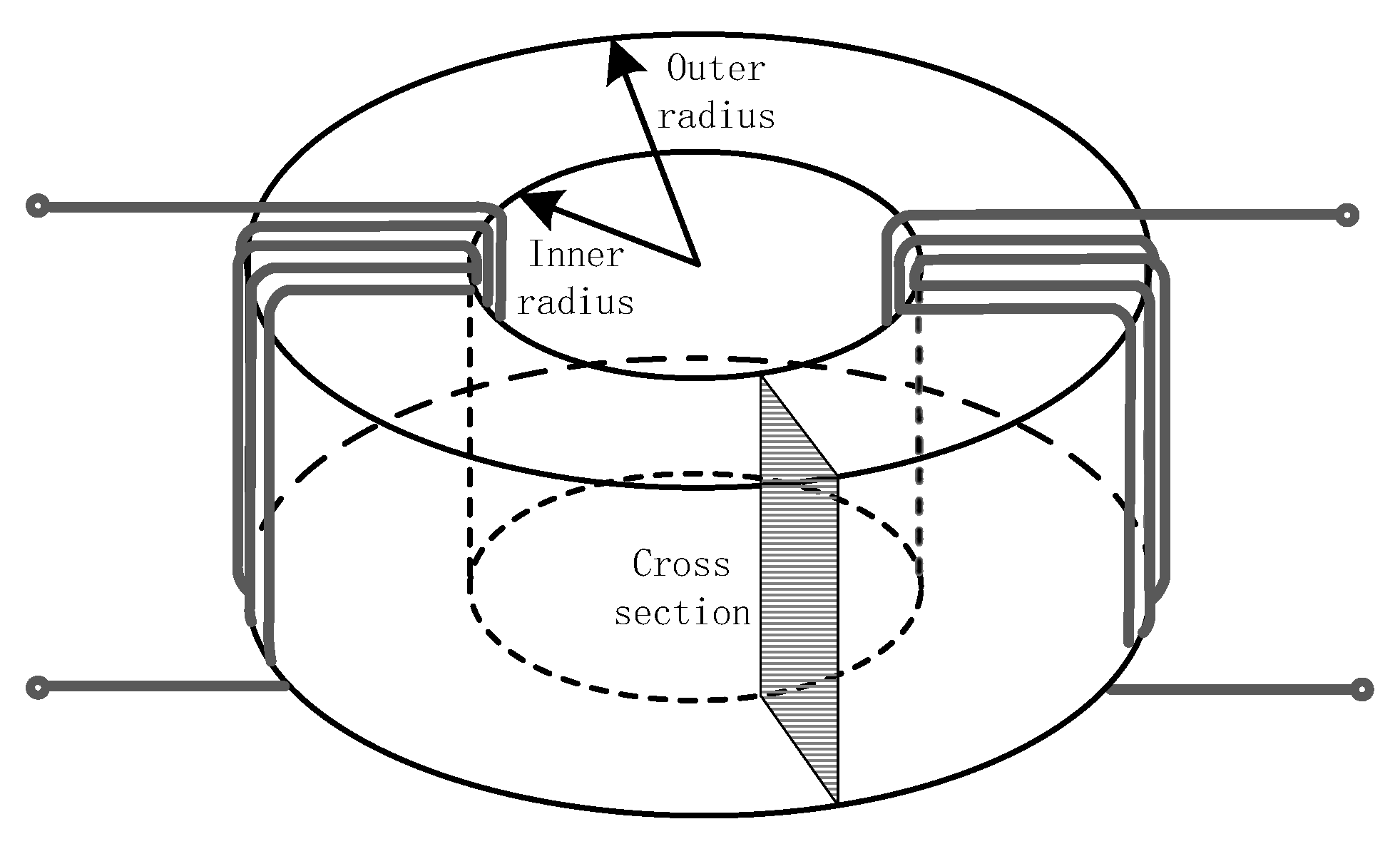
The structure of the toroidal magnetic core is simple and can be directly analyzed and calculated using the method shown in Section 3. It is worth noting that the cross-section shown in Figure 3 needs to be solved separately in the transverse and longitudinal directions using the method described in Section 3.
4.2. Consideration of Excess Loss and Influence of Skin Effect on Magnetic Permeability μ
In Bertotti’s loss separation model, the core loss P is divided into three parts:
where Physt is the hysteresis loss, Peddy is the eddy current loss, and Pexc is the excess loss and also known as the excess eddy current loss. The excess loss is usually considered as the difference between the measured core loss and the calculated hysteresis loss and eddy current loss. Therefore, additional experimental measurements are usually required to obtain the excess loss. The excess loss is explained by Bertotti’s statistical loss theory as the change in magnetic flux density due to the random distribution of domain wall motion. Based on the statistical loss theory, it is considered to be in direct proportion to f1.5 and B1.5. However, Bertotti’s statistical loss theory is based on the assumption that the magnetic field is uniformly distributed [30], which ignores different magnetic circuit lengths, skin effects, and the uneven distribution of magnetic characteristic parameters. In another views, excess losses are attributed to the peculiar nature of nonlinear electromagnetic field diffusion in the lamination [31,32], which means that the uneven distribution of magnetic flux density leads to the excess loss. Because the excess loss coefficient in the statistical loss theory is difficult to characterize and reflect its reaction to the magnetic field, this paper uses the second explanation to consider the excess loss.
Experimental measurements or material data manuals usually offer the average magnetic permeability of the magnetic core. In fact, the magnetic permeability inside the magnetic core is not uniform, and it is difficult to obtain the magnetic permeability distribution at different positions inside the magnetic core. A hypothetical phenomenon of “concentration effect” for toroidal magnetic cores is proposed in [25], and this article still uses this approach to consider the uneven distribution of magnetic flux density and permeability. Differently, the skin effect is not considered in [25]. In order to simplify the equation and reduce parameters, the expression for magnetic flux density in (24) is used in this article to consider the skin effect. The equation is:
where Bavg represents the average magnetic flux density inside the magnetic core. The constant coefficient needs to know the partial loss data of the specific magnetic core within the studied frequency range, including at least the data at both ends of the range. Based on the loss results and the loss calculation method, the specific value of coefficient can be reversibly derived. When the frequency range is wide, this coefficient may also be a polynomial that varies with frequency [25], and within the scope of this article, this coefficient is a constant.
5. Validation
5.1. Distribution of Magnetic Flux Density in Magnetic Cores
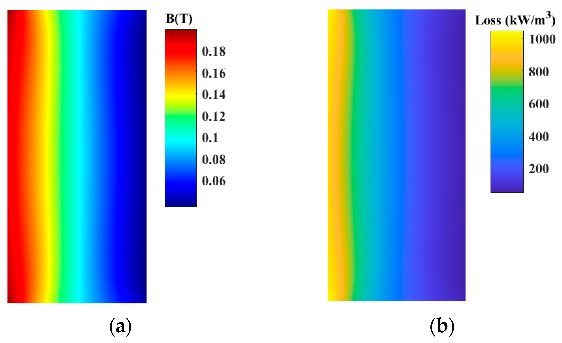
To verify the feasibility of the proposed method in this article, according to the analytical calculation equations described in Section 3, the average magnetic flux density distribution on the outer surface and cross-section of 3E6 at frequencies of 100 kHz and 400 kHz is shown in Figure 6, where the rectangular box on the right is the cross-section of the magnetic core shown in Figure 3.
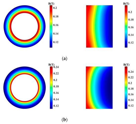
Figure 6.
The average magnetic flux density distribution on the outer surface view and cross-section view of the magnetic core 3E6 obtained using the proposed method. (a) 100 kHz. (b) 400 kHz.
From Figure 6, it can be seen that the proposed method in this article clearly demonstrates the uneven distribution of magnetic flux density in the magnetic core 3E6 under high frequency. In addition, comparing Figure 6a,b, it can be seen that as the frequency increases, the magnetic flux concentrates inward further, and the maximum magnetic flux density inside the magnetic core is higher. Additionally, the magnetic flux is more concentrated on the surface of the magnetic core, leading to uneven distribution of magnetic flux density.
The same material, size, electromagnetic properties, and other parameters are also modeled using ANSYS simulation software (Version 2023 R2), as shown in Figure 7.
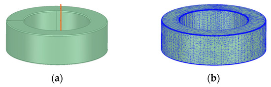
Figure 7.
ANSYS simulation model of 3E6 magnetic core. (a) 3-D model. (b) Mesh generation.
The same boundary conditions as the analytical model are set. Through the eddy current field simulation of ANSYS, the simulation results at 100 kHz and 400 kHz can be obtained, as shown in Figure 8. The relative permeability is set to “nonlinear” in the ANSYS material setting. The magnetic core is set to consider “skin effect” and “core loss” in the ANSYS excitation setting.
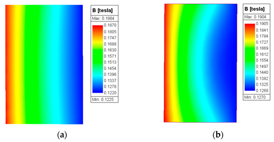
Figure 8.
The average magnetic flux density distribution on the cross-section view of the magnetic core obtained using ANSYS. (a) 100 kHz. (b) 400 kHz.
It can be seen from Figure 8 that the simulation results of ANSYS also show the influence of frequency on the uneven distribution of magnetic flux density, which is similar to Figure 6. However, the difference is that the degree of uneven distribution of magnetic flux density in Figure 8 is smaller than that in Figure 6. The main reason is that ANSYS does not consider the “concentration effect” as the method in this paper.
5.2. Distribution of Core Losses in Magnetic Cores
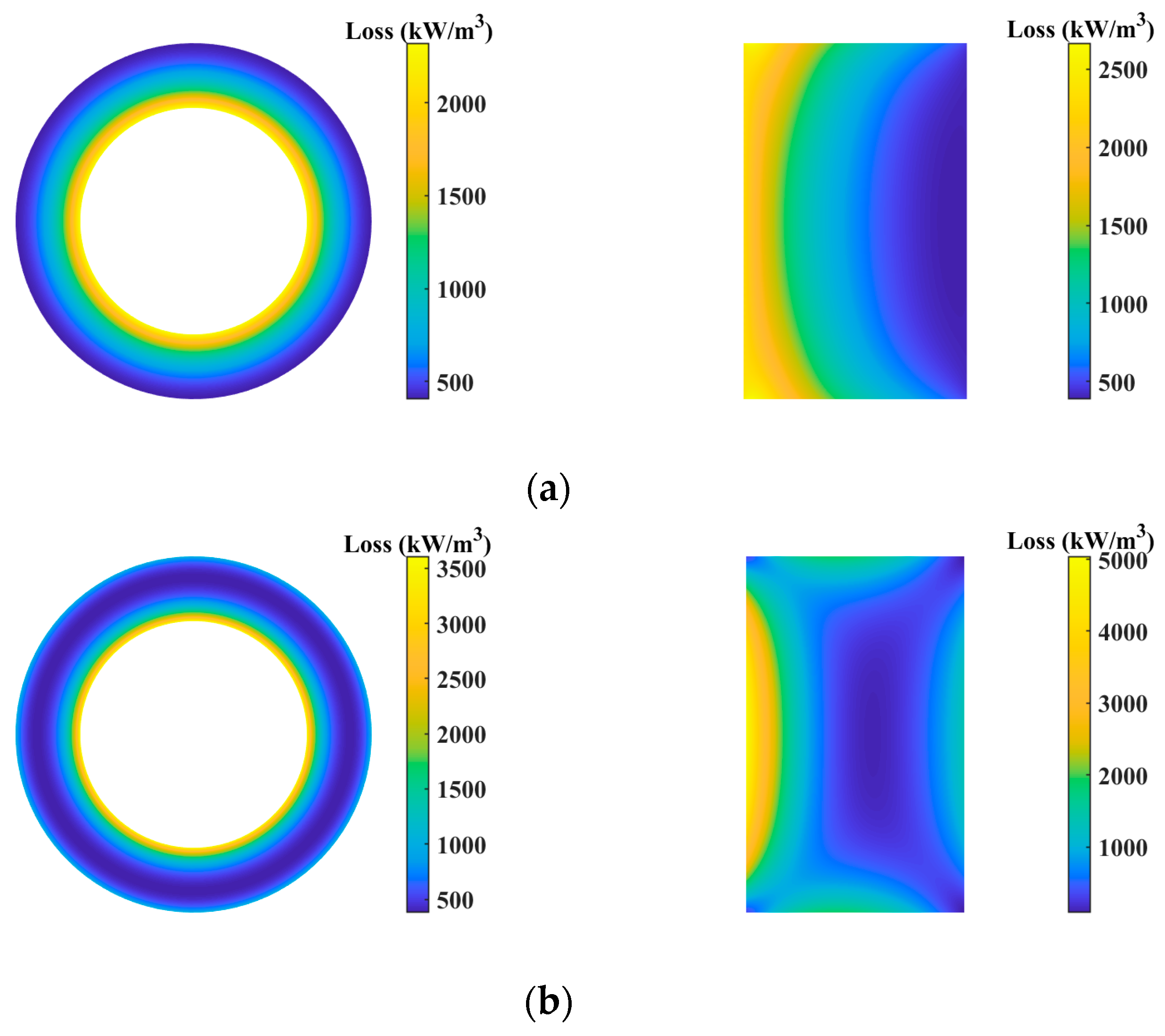
For the 400 kHz case, according to the proposed method, the distribution of hysteresis loss, eddy current loss, and total loss density (kW/m3) on the magnetic core and cross-section is shown in Figure 9.


Figure 9.
The distribution of loss density (kW/m3) on the magnetic core 3E6 and cross-section by the proposed method at 400 kHz. (a) Hysteresis loss. (b) Eddy current loss. (c) Total loss.
The outer surface and cross-section in Figure 9 show the average power loss distribution of the entire magnetic core. Due to the special structure and skin effect phenomenon [33] of the toroidal magnetic core, it can be seen that eddy current losses and hysteresis losses also exhibit a characteristic of concentrating toward the inner ring and the surface. What is more, the proposed method can demonstrate the uneven distribution of hysteresis loss and eddy current loss within the magnetic core, respectively. The skin effect of eddy current losses under high-frequency conditions can also be reflected in the final magnetic core losses.
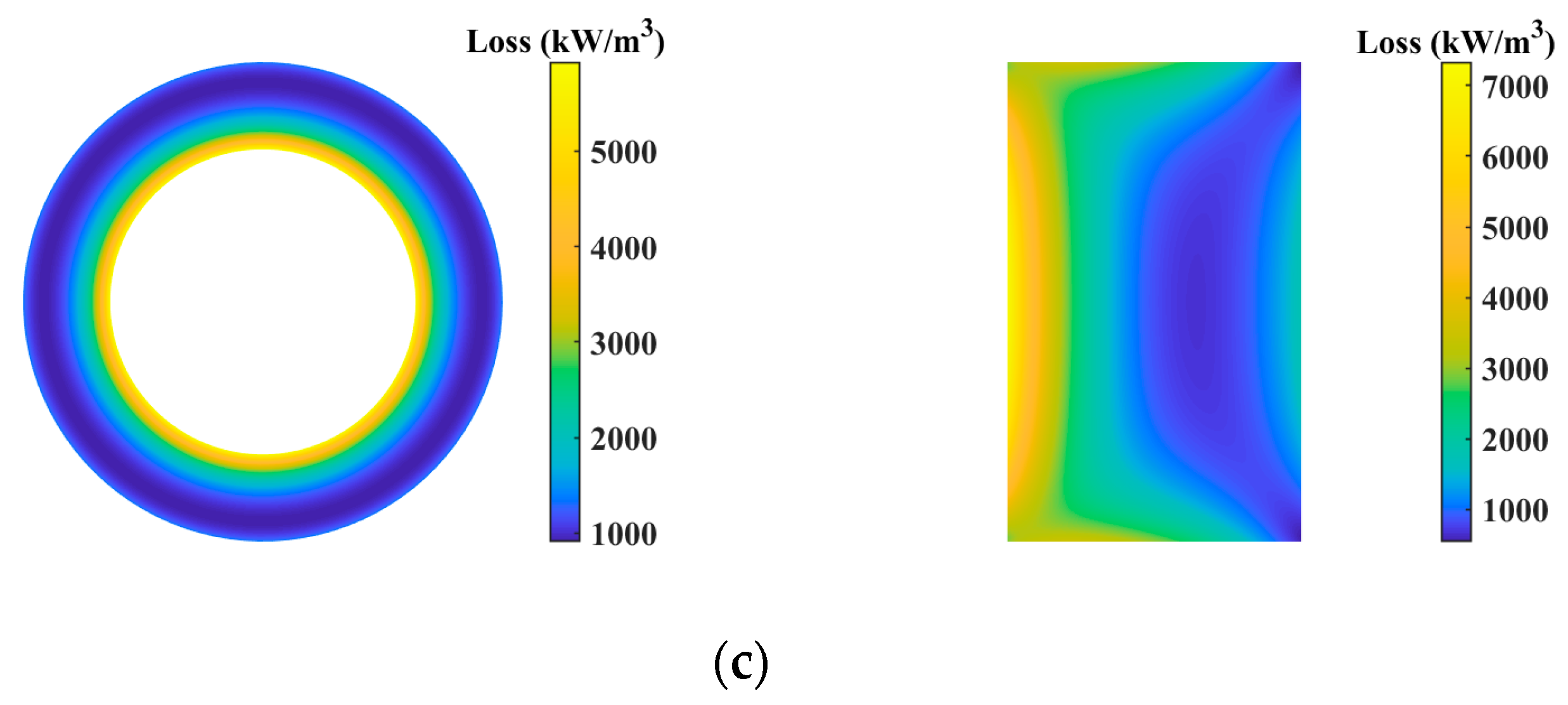
The simulation results for the same 400 kHz case using ANSYS software (Version 2023 R2) are shown in Figure 10. However, ANSYS does not consider the effect of hysteresis on the magnetic field, as described in this article, so ANSYS cannot give the calculation results of hysteresis loss. In Figure 10, “OhmicLoss” is the eddy current loss calculated by ANSYS software, and “CoreLoss” is the core loss calculated using ANSYS software. Among the magnetic core loss calculation models built in ANSYS, the “power ferrite” model is the most suitable for 3E6 and N87 and has been chosen for comparison in this paper.
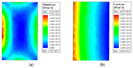
Figure 10.
The distribution of loss density (kW/m3) on the magnetic core 3E6 obtained using ANSYS at 400 kHz. (a) Ohmicloss. (b) CoreLoss. The coefficients of the “power ferrite” loss model are Cm = 0.0058, X = 1.8702, and Y = 2.1475.
The eddy current loss distribution and the total loss distribution similar to those in Figure 9 are shown in Figure 10. The difference is the degree of unevenness, which is still caused by the uneven distribution of magnetic permeability. However, more importantly, the calculation of core loss using ANSYS software is in the post-processing phase, and the result of loss calculation depends more on the coefficients of the adopted loss model. Comparing Figure 10a,b, the eddy current skin effect observed in 3E6 at 400 kHz was not considered by ANSYS in the final core loss. In addition, if the coefficients of the loss model are simply changed, the result is shown in Figure 11.
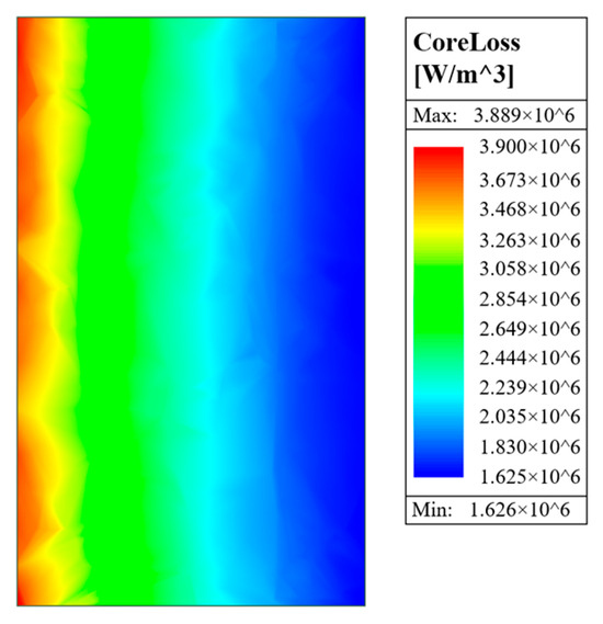
Figure 11.
The distribution of loss density (kW/m3) on the magnetic core 3E6 obtained using ANSYS at 400 kHz. The different coefficients of the “power ferrite” loss model are Cm = 0.0007, X = 2, and Y = 2.0254.
Figure 11 shows the loss density distribution of 3E6 by ANSYS at 400 kHz under the different coefficients of the “power ferrite” loss model based on the magnetic flux distributions in Figure 8, the same as those for Figure 10. The same material properties and magnetic field distribution result in different loss values just due to different loss coefficients, which further confirms the independence between electromagnetic field analysis and loss calculation in ANSYS simulation. Therefore, the reaction of hysteresis, eddy current, and excess loss to the magnetic field is also not quantitatively considered by ANSYS.
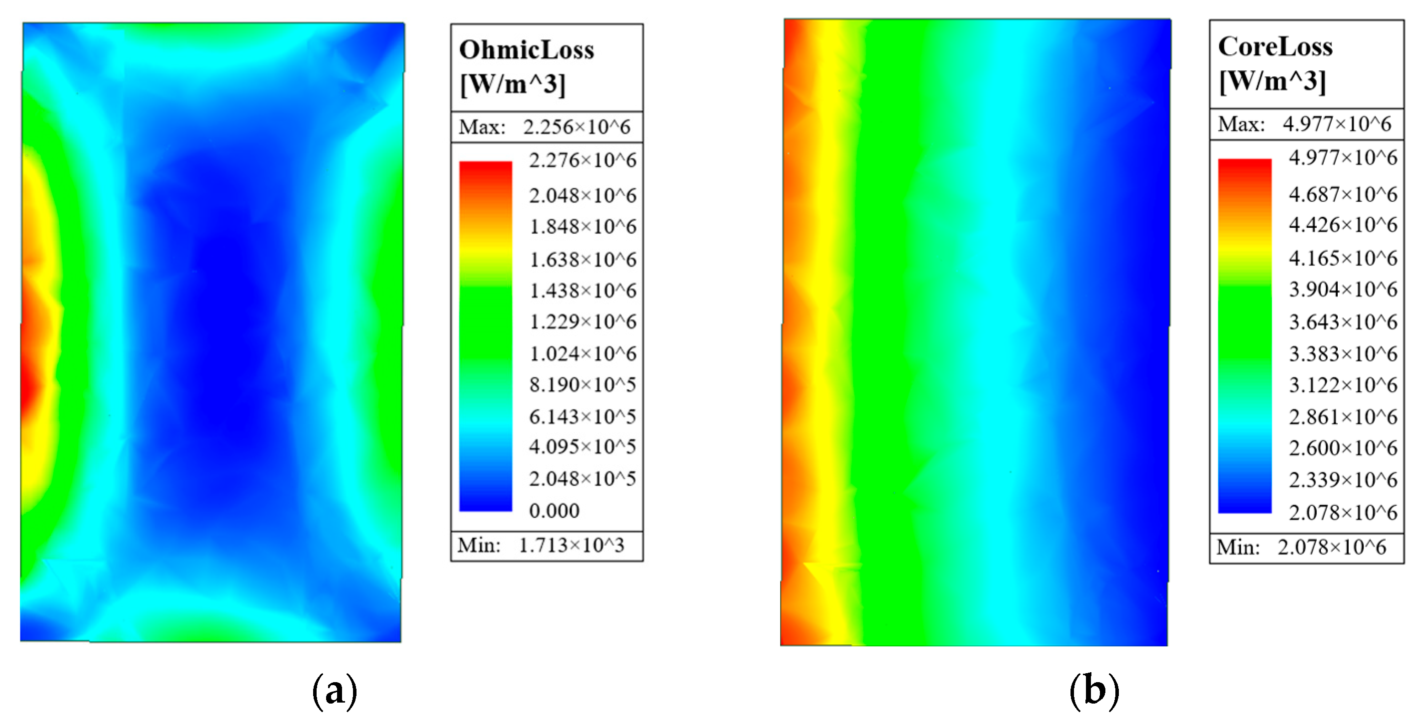
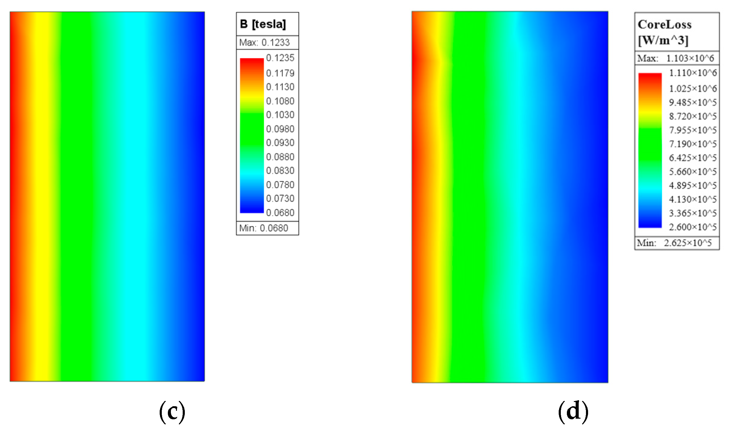
For the N87 magnetic core at 300 kHz under identical conditions, the analytical and simulation results are presented, as shown in Figure 12.

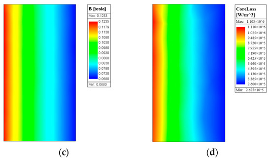
Figure 12.
The magnetic flux density and core loss distribution of N87 at 300 kHz condition. (a) Magnetic flux density distribution obtained using analytical calculation. (b) Core loss distribution obtained using analytical calculation. (c) Magnetic flux density distribution obtained via ANSYS simulation. (d) Core loss distribution obtained via ANSYS simulation. The coefficients of the “power ferrite” loss model for N87 are Cm = 12.8258, X = 1.3453, and Y = 2.5752.
Compared to 3E6, it can be seen from Figure 12 that there will be much less skin phenomena in N87, even under high-frequency conditions of 300 kHz. The reason is that the conductivity of N87 is very low, which can be obtained from Table 2. However, the structure of the toroidal core still causes an uneven distribution of magnetic flux in the cross-section, resulting in uneven distributions of magnetic permeability and hysteresis angle, which should be considered when calculating hysteresis losses and excess losses.
Table 2.
Comparison of experimental data Ex_PV, calculated data of the proposed method Cal_PV, and ANSYS simulation data ANSYS_ PV of 3E6 (kW/m3).
5.3. Calculation and Comparison of Core Losses
In order to verify the correctness and accuracy of the method proposed in this paper, the core loss obtained by analysis Cal_PV is compared with the experimental value Ex_PV and ANSYS simulation value ANSYS_PV in Table 2. In addition, Cal_Ph and Cal_Pe, respectively, represent the hysteresis loss and eddy current loss calculated using the method proposed in this article. The experimental data can be obtained from [34].
From Table 2, it can be obtained that the average error between the proposed method and the experiments is 3.6%, while the average error between the ANSYS simulation and the experiments is 17.2%. Obviously, the proposed method in this article has much better accuracy. Furthermore, at 400 kHz, the error of ANSYS simulation results is significantly higher than that at 200 kHz. The main reason is that the loss coefficients of the “power ferrite” loss model are fitted based on the average magnetic flux density, and it is assumed that the magnetic flux density of the magnetic core is uniform. However, as shown in Figure 8, under high-frequency conditions, the distribution of magnetic flux density inside the magnetic core is very uneven. Therefore, the coefficients of the “power ferrite” loss model did not take into account the high-frequency skin effect and uneven distribution of magnetic flux, and the electromagnetic field analysis did not quantitatively consider the reaction of hysteresis, eddy currents, and residual loss on the magnetic field. The independence of the magnetic field calculation and loss calculation will lead to significant errors in the loss calculation. Conversely, the proposed method directly introduces hysteresis angle parameters and non-uniform magnetic permeability into the electromagnetic field analysis equation. Combining the reaction of eddy currents on magnetic fields and the phase effect of hysteresis on B and H, specific eddy current losses and hysteresis losses can be calculated, and more accurate magnetic core losses can be obtained.
For the N87 magnetic core, the comparison results of core loss under different conditions are shown in Table 3.
Table 3.
Comparison of experimental data Ex_PV, calculated data of the proposed method Cal_PV, and ANSYS simulation data ANSYS_ PV of N87 (kW/m3).
In Table 3, it can be seen that the average error between the proposed method and the experiments is 4.6%, while the average error between the ANSYS simulation and the experiments is 8.6%. Similarly, the proposed method in this article has better accuracy. However, unlike the magnetic core 3E6, the skin effect of N87 is relatively weak, and the reaction of eddy currents to the magnetic field is also weak. Although appropriate coefficients of the “power ferrite” loss model can also obtain relatively good calculation values, the problem of electromagnetic field analysis and loss calculation being independent of each other still exists. The calculation results of the loss of N87 are mainly aimed at verifying the universality of the proposed method.
6. Conclusions
In this paper, a new two-dimensional electromagnetic field analysis and loss calculation method for high-frequency applications has been proposed based on vector magnetic circuit theory. The physical concept of hysteretance and magductance originated from the vector magnetic circuit theory provides a different prospective and modeling method for analyzing magnetic characteristics and predicting power loss in magnetic circuits. The effect of eddy currents on magnetic fields is considered through the influence of current density on magnetic field strength, while the effect of hysteresis on magnetic fields is characterized by the hysteresis angle between magnetic flux density and magnetic field strength. The uneven distribution of magnetic permeability caused by the uneven distribution of magnetic fields is also taken into account in the proposed method. Therefore, the loss value that matches the reaction caused by eddy currents and hysteresis on the magnetic field can be accurately calculated. By comparing with the experimental values and ANSYS simulation values, the accuracy and effectiveness of the proposed method have been verified.
Author Contributions
Conceptualization, M.C. and C.L.; methodology, C.L.; software, C.L.; validation, C.L.; formal analysis, C.L.; investigation, C.L.; resources, C.L.; data curation, C.L.; writing—original draft preparation, C.L.; writing—review and editing, M.C. and W.W.; visualization, C.L.; supervision, M.C. and W.W.; project administration, M.C.; funding acquisition, M.C. All authors have read and agreed to the published version of the manuscript.
Funding
This research was funded by National Natural Science Foundation of China grant number [52450007] and Postgraduate Research&Practice Innovation Program of Jiangsu Province grant number [KYCX24_0397].
Data Availability Statement
The original contributions presented in this study are included in the article. Further inquiries can be directed to the corresponding author.
Conflicts of Interest
The authors declare no conflict of interest.
References
- Silveyra, J.M.; Ferrara, E.; Huber, D.L.; Monson, T.C. Soft magnetic materials for a sustainable and electrified world. Science 2018, 362, eaao0195. [Google Scholar] [CrossRef] [PubMed]
- 2023 IEEE International MagNet Challenge, 2023 MagNet Challenge Handbook. Available online: https://github.com/minjiechen/magnetchallenge/blob/main/docs/handbook.pdf (accessed on 3 March 2023).
- Cui, H.H.; Dulal, S.; Sohid, S.B.; Gu, G.; Tolbert, L.M. Unveiling the microworld inside magnetic materials via circuit models. IEEE Power Electron. Mag. 2023, 10, 14–22. [Google Scholar] [CrossRef]
- Serrano, D.; Li, H.; Wang, S.; Guillod, T.; Luo, M.; Bansal, V.; Jha, N.K.; Chen, Y.; Sullivan, C.R.; Chen, M. Why MagNet: Quantifying the complexity of modeling power magnetic material characteristics. IEEE Trans. Power Electron. 2023, 38, 14292–14316. [Google Scholar] [CrossRef]
- Mu, M.; Zheng, F.; Li, Q.; Lee, F.C. Finite element analysis of inductor core loss under DC bias condition. In Proceedings of the 2012 Twenty-Seventh Annual IEEE Applied Power Electronics Conference and Exposition (APEC), Orlando, FL, USA, 5–9 February 2012; pp. 405–410. [Google Scholar] [CrossRef]
- Yamazaki, K.; Fukushima, N. Torque and loss calculation of rotating machines considering laminated cores using post 1-D analysis. IEEE Trans. Magn. 2011, 47, 994–997. [Google Scholar] [CrossRef]
- Courtay, A. The Preisach Model; Analogy Inc.: Austin, TX, USA, 1999. [Google Scholar]
- Jiles, D.C.; Atherton, D.L. Theory of ferromagnetic hysteresis. J. Magn. Magn. Mater. 1986, 61, 48–60. [Google Scholar] [CrossRef]
- Mu, M.; Li, Q.; Gilham, D.J.; Lee, F.C.; Ngo, K.D.T. New core loss measurement method for high-frequency magnetic materials. IEEE Trans. Power Electron. 2014, 29, 4374–4381. [Google Scholar] [CrossRef]
- Lawton, P.A.J.; Lin, F.J.; Covic, G.A. Magnetic design considerations for high-power wireless charging systems. IEEE Trans. Power Electron. 2022, 37, 9972–9982. [Google Scholar] [CrossRef]
- Fallah, E.; Moghani, J.S. A New Approach for Finite-Element Modeling of Hysteresis and Dynamic Effects. IEEE Trans. Magn. 2006, 42, 3674–3681. [Google Scholar] [CrossRef]
- Sadowski, N.; Batistela, N.J.; Bastos, J.P.A.; Lajoie-Mazenc, M. An inverse Jiles-Atherton model to take into account hysteresis in time-stepping finite-element calculations. IEEE Trans. Magn. 2002, 38, 797–800. [Google Scholar] [CrossRef]
- Fallah, E.; Badeli, V. A New Approach for Modeling of Hysteresis in 2-D Time-Transient Analysis of Eddy Current Using FEM. IEEE Trans. Magn. 2017, 53, 1–14. [Google Scholar] [CrossRef]
- Leonard, P.J.; Marketos, P.; Moses, A.J.; Lu, M. Iron losses under PWM excitation using a dynamic hysteresis model and finite elements. IEEE Trans. Magn. 2006, 42, 907–910. [Google Scholar] [CrossRef]
- Patsios, C.; Tsampouris, E.; Beniakar, M.; Rovolis, P.; Kladas, A.G. Dynamic finite element hysteresis model for iron loss calculation in non-oriented grain iron laminations under PWM excitation. IEEE Trans. Magn. 2011, 47, 1130–1133. [Google Scholar] [CrossRef]
- Ceylan, D.; Zeinali, R.; Daniels, B.; Boynov, K.O.; Lomonova, E.A. A Novel modeling technique via coupled magnetic equivalent circuit with vector hysteresis characteristics of laminated steels. IEEE Trans. Ind. Appl. 2023, 59, 1481–1491. [Google Scholar] [CrossRef]
- Soda, N.; Enokizono, M. Improvement of T-joint part constructions in three-phase transformer cores by using direct loss analysis with E&S model. IEEE Trans. Magn. 2000, 36, 1285–1288. [Google Scholar] [CrossRef]
- Enokizono, M. Vector magnetic property and magnetic characteristic analysis by vector magneto-hysteretic E&S model. IEEE Trans. Magn. 2009, 45, 1148–1153. [Google Scholar] [CrossRef]
- Xie, D.; Yang, S. Numerical Analysis and Optimization of Engineering Electromagnetic Fields; China Machine Press: Beijing, China, 2017; pp. 147–185. [Google Scholar]
- Silvester, P.P.; Ferrari, R.L. Finite Elements for Electrical Engineers, 3rd ed.; Cambridge University Press: Cambridge, UK, 1996; pp. 344–403. [Google Scholar]
- Kacki, M.; Rylko, M.S.; Hayes, J.G.; Sullivan, C.R. A high-performance EMI filter based on laminated ferrite ring cores. In Proceedings of the 2022 24th European Conference on Power Electronics and Applications (EPE’22 ECCE Europe), Hanover, Germany, 5–9 September 2022; pp. 1–7. [Google Scholar]
- Lin, D.; Zhou, P.; Fu, W.N.; Badics, Z.; Cendes, Z.J. A dynamic core loss model for soft ferromagnetic and power ferrite materials in transient finite element analysis. IEEE Trans. Magn. 2004, 40, 1318–1321. [Google Scholar] [CrossRef]
- ANSYS. Introduction to Icepak in AEDT. Available online: https://innovationspace.ansys.com/courses/wpcontent/uploads/sites/5/2021/07/AEDT_Icepak_Int_2020R1_EN_LE01.1.pdf (accessed on 5 July 2020).
- Cheng, M.; Qin, W.; Zhu, X.; Wang, Z. Magnetic-inductance: Concept, definition, and applications. IEEE Trans. Power Electron. 2022, 37, 12406–12414. [Google Scholar] [CrossRef]
- Li, C.; Cheng, M.; Qin, W.; Wang, Z.; Ma, X.; Wang, W. Analytical loss model for magnetic cores based on vector magnetic circuit theory. IEEE Open J. Power Electron. 2024, 5, 1659–1670. [Google Scholar] [CrossRef]
- Li, C.; Qin, W.; Wang, Z.; Ma, X.; Wang, W.; Cheng, M. Core loss model for non-sinusoidal excitations based on vector magnetic circuit theory. In Proceedings of the International Conference on Electrical Machines (ICEM), Torino, Italy, 1–4 September 2024; pp. 1–6. [Google Scholar] [CrossRef]
- Salon, S.J.; Chari, M.V.K.; Ergene, L.T.; Burow, D.; DeBortoli, M. Eddy Currents: Theory, Modeling and Applications; Wiley-IEEE Press: New York, NY, USA, 2023; pp. 45–129. [Google Scholar]
- FERROXCUBE. Material Specification 3E6 (3E10-M). Available online: https://www.ferroxcube.com/upload/media/product/file/MDS/3e6.pdf (accessed on 18 November 2016).
- TDK. SIFERRIT Material N87. Available online: https://www.tdk-electronics.tdk.com/download/528882/990c299b916e9f3eb7e44ad563b7f0b9/pdf-n87.pdf (accessed on 22 February 2023).
- Bertotti, G. General properties of power loss in soft ferromagnetic materials. IEEE Trans. Magn. 1988, 21, 621–630. [Google Scholar] [CrossRef]
- Serpico, C.; Visone, C.; Mayergoyz, I.D.; Basso, V.; Miano, G. Eddy current losses in ferromagnetic laminations. J. Appl. Phys. 2000, 87, 6923–6925. [Google Scholar] [CrossRef]
- Mayergoyz, I.; Serpico, C. Nonlinear diffusion of electromagnetic fields and excess eddy current losses. J. Appl. Phys. 1999, 85, 4910–4912. [Google Scholar] [CrossRef]
- Cheng, M.; Qin, W.; Zhu, X.; Wang, Z.; Hua, W. High-performance breathable magnetic core for high-frequency power electronic systems. Fundam. Res. 2024. [Google Scholar] [CrossRef]
- Li, H.; Serrano, D.; Wang, S.; Chen, M. MagNet-AI: Neural network as datasheet for magnetics modeling and material recommendation. IEEE Trans. Power Electron. 2023, 38, 15854–15869. [Google Scholar] [CrossRef]


Disclaimer/Publisher’s Note: The statements, opinions and data contained in all publications are solely those of the individual author(s) and contributor(s) and not of MDPI and/or the editor(s). MDPI and/or the editor(s) disclaim responsibility for any injury to people or property resulting from any ideas, methods, instructions or products referred to in the content. |
© 2025 by the authors. Licensee MDPI, Basel, Switzerland. This article is an open access article distributed under the terms and conditions of the Creative Commons Attribution (CC BY) license (https://creativecommons.org/licenses/by/4.0/).