Bounding Case Requirements for Power Grid Protection Against High-Altitude Electromagnetic Pulses

Abstract

Securing the power grid is of extreme concern to many nations as power infrastructure has become integral to modern life and society. A high-altitude electromagnetic pulse (HEMP) is generated by a nuclear detonation high in the atmosphere, producing a powerful electromagnetic field that can damage or destroy electronic devices over a wide area. Protecting against HEMP attacks (insults) requires knowledge of the problem’s bounds before the problem can be appropriately solved. This paper presents a collection of analyses to determine the basic requirements for controller placements on a power grid. Two primary analyses are conducted. The first is an inverted controllability analysis in which the HEMP event is treated as an unbounded control input to the system. Considering the HEMP insult as a controller, we can break down controllability to reduce its influence on the system. The analysis indicates that either all but one neutral path to ground must be protected or that all transmission lines should be secured. However, further exploration of the controllability definition suggests that fewer blocking devices are sufficient for effective HEMP mitigation. The second analysis involves observability to identify the minimum number of sensors needed for full-state feedback. The results show that only one state sensor is required to achieve full-state feedback for the system. These requirements suggest that there is room to optimize controller design and placement to minimize total controller count on a power grid to ensure HEMP mitigation. As an example, the Horton et al. system model with 15 transformers and 15 transmission lines is used to provide a baseline comparison for future optimization studies by running all permutations of neutral and transmission line blocking cases. The minimum number of neutral controllers is 8, which is approximately half of the bounding solution of 14. The minimum number of transmission line controllers is 3, which is one-fifth of the bounding solution of 15 and less than half of the required neutral controllers.

1. Introduction

Growing national security concerns have led to an increased interest in HEMP mitigation strategies to ensure national power grid resilience [1,2]. The nature of HEMP insults will be explained in the System Models section of this paper, but at the most fundamental level, an HEMP insult is generated by the detonation of a nuclear device in the atmosphere. The HEMP insult couples with transmission lines and induces unwanted current. This energy injection can be large enough to saturate transformers and degrade power quality. This can lead to loss of substations and rolling blackouts. There have been several recorded instances of geomagnetic disturbances and HEMP insults influencing the power grid.

A reported instance of power grid interference due to an HEMP insult occurred during the Starfish Prime high-altitude nuclear test [3]. The failure of 30 series connected loops of street lights at various locations on the island of Oahu was traced back to the detonation of a nuclear device nearby. The island itself was located approximately 800 mi away from ground zero of the detonation. While the failure itself was not initially considered major, it does provide some insight into the mechanics of HEMP coupling. The lighting circuits that were impacted by the HEMP insult consisted of 3000 ft long horizontal loops, approximately 14.5 in wide [4]. This suggests that properly aligned conductors as short as 3000 ft (or approx 1 km) could couple with an HEMP insult from over 1000 km away. The test occurred more than 60 years ago near a power grid with relatively short transmission lines. On the modern grid, in a more densely populated area, the results could be significantly more damaging. As such, there is a need to harden the power grid against HEMP insults.

This paper assesses the requirements for various control techniques in the mitigation of HEMP insults on the power grid, with an emphasis on protecting conventional transformers. In particular, the primary goal of this paper is to lay out the bounding case requirements for HEMP mitigation. The impetus for the optimization problem is developed and presented. Historically, the optimal device placement problem has been performed without defining the bounding case requirements [5,6,7]. In response, this paper derives and presents the bounding requirements.

This analysis is broken into two main components. The first component utilizes controllability to define the system requirements for removing HEMP influence from the system in its entirety. The second component looks at observability and the required number of sensors to enable the use of state estimators to reduce the number of required sensors for global control (i.e., full state feedback). Controllability is defined and used as a metric to determine the bounds of a disturbance as an input. This analysis is performed to determine how unwanted power is able to flow through an electric grid. An observability analysis is then performed to generate bounds on the required number of sensors to perform state estimation. This generates requirements on information flow and allows for the further development of a Kalman filter for full-state estimation.

Previous controllability analysis on the power grid has been performed on the controllers themselves as the inputs [8]. While this provides information on how a controller (or set of controllers) is able to move power around and affect the states of devices through the power grid, it fails to provide information on the nature of the HEMP coupling itself. By treating the disturbance as a controller itself, the disturbance influence controllability study states what must be performed in order to remove all influence of the HEMP insult from the system. Unlike most of the literature on the topic [9,10,11,12,13,14], this study is performed using actively controlled energy storage devices to derive system specifications [8,15,16]. Passive capacitors act as integrator controllers and, as such, will not remove energy from a system. Additionally, the capacitors raise the order of the transformer subsystems by one, further enabling ringing from highly impulsive portions of the HEMP insult.

In addition to the controllability study, an observability study is performed. These results are used to determine the minimum number of required sensors to ensure that an observer is able to estimate the full state of the power grid system. Some work has been carried out in ensuring and improving power grid observability [17,18]. This observability study is performed in this paper as a framework for future work in grid state estimation. It will be shown that global controls on the transmission line side of a substation provide more redundancy than the local transmission line controller. However, there may be constraints around the communications and so there may be a beneficial trade-off in the relaxation of communications requirements for additional computational power. The observability study provides requirements for the minimum number of sensors for the implementation of a Kalman filter as an observer.

This paper is broken into seven main sections. Section 1 consists of an introduction and motivation for solving the problem of HEMP mitigation device placements. Section 2 section consists of descriptions of the system models, including characterization of the late-time HEMP insult and definition of the power grid model. Section 3 develops the control law used. Additionally, this section states why the specific control law was chosen over traditional passive capacitor solutions. Section 4 introduces the most fundamental definition of controllability and how it pertains to the HEMP influence problem. Section 4 explains how the definition of controllability may be used to apply bounds to the placement problem. In particular, the definition of controllability is used to state how system inputs map to system outputs. Section 5 introduces the fundamental definition of system observability and how system knowledge may be exploited to lessen the required number of sensors in a power grid to mitigate an HEMP insult. Section 6 presents the all-permutation results for 16 different HEMP field orientations and neutral and transmission line blocking device utilization. This is all possible combinations of homogeneous placements (i.e., all neutral blocking devices or all transmission line blocking devices) on the power grid and the worst absolute magnetic core flux value as a baseline comparison for future optimization studies. Section 7 provides a conclusion of the work presented in this paper. The results from this paper will be used to set up the optimization problem for optimal control placement and high-level control design in future work as a follow on [19,20,21].

2. System Models

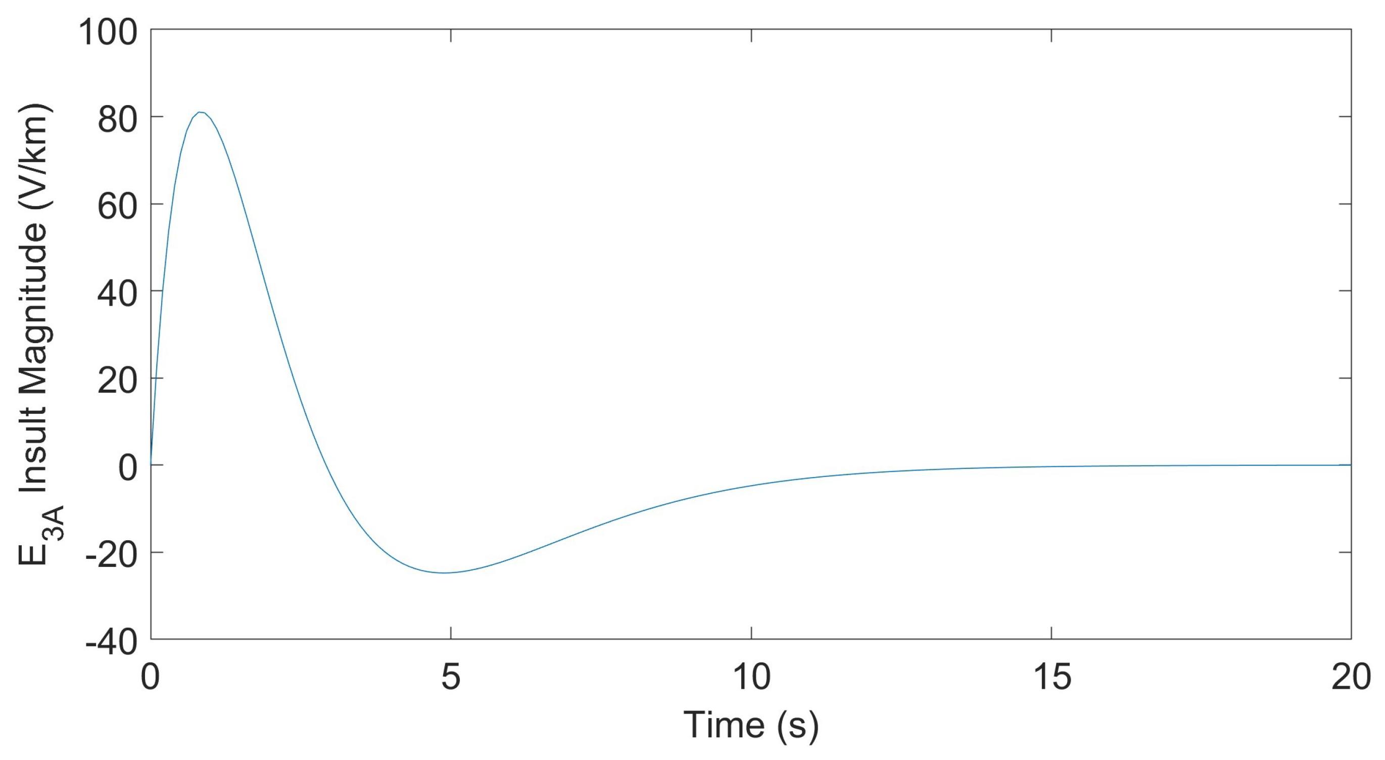
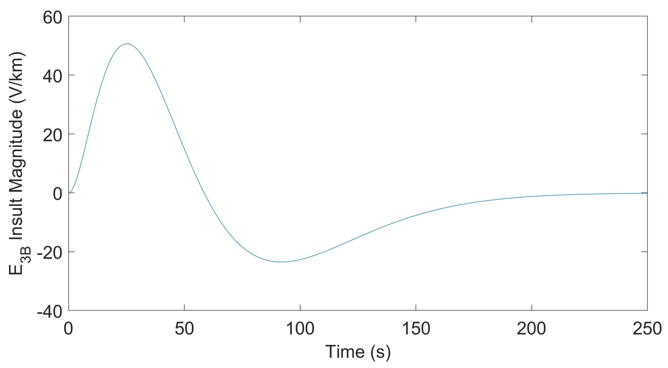
2.1. HEMP Insult Model

HEMP insults are generated by the detonation of nuclear devices in the Earth’s atmosphere, often at an altitude of 40 km or greater [22]. HEMP insults, when compared to naturally occurring geomagnetic disturbances from coronal mass ejections and space weather, tend to have overall larger amplitudes and higher frequencies. The exact nature of the HEMP field is highly dependent on asymmetries present in the source (i.e., nuclear detonation), nonuniformity of the Earth’s magnetic field, and gradients in the Earth’s atmospheric density.

The HEMP insult comprises three main time domains. The first time domain of the HEMP insult is labeled as the $E_1$ portion. According to IEC Standard 1000-2-9, the $E_1$ portion of the insult occurs for the first 0.1 μs after the detonation of a nuclear device in the atmosphere [23]. This portion of the insult may generate voltage potentials along transmission lines >10 kV/m. Following the $E_1$ component is the $E_2$ component of the HEMP insult. This insult is defined to end 1 s after the initial detonation [23]. The resulting potential across transmission lines due to the HEMP field is on the order of 100 V/m.

The last time component of the HEMP signal is the $E_3$ component and it is further broken into two sub-components. This part of the HEMP insult lasts from 1 s after the detonation to 250 s after the detonation. The $E_{3A}$ portion, or “blast“, consists of a somewhat impulsive potential field that peaks slightly higher than the potential field of the $E_{3B}$ component, approximately around 100 V/km, and then settles down. The $E_{3B}$, or “heave“ portion of the HEMP insult occurs at an even lower frequency than the $E_{3A}$ portion [24]. As a result, this portion of the $E_3$ insult is sometimes treated as a DC signal [25,26]. In [27], the best fit characterization of the $E_{3A}$ portion is given as

$$E_{3A}=\alpha e^{-t/\beta }(\gamma t-\delta t^2)$$

(1)

where $\alpha =9.5$, $\beta =1.4$, $\gamma =26$, and $\delta =8.9$. The corresponding plot of (1) is shown in Figure 1. Additionally, the $E_{3B}$ portion of the insult is given as

$$E_{3B}=-\alpha t^2{e}^{-t/\gamma }{\displaystyle \frac{{\beta }^{3}t-3{\beta }^3\gamma +t^4}{\gamma {({\beta }^3+t^3)}^2}}$$

(2)

where $\alpha =1.3·{10}^6$, $\beta =200$, and $\gamma =20$. The corresponding plot of (2) is shown in Figure 2.

The strength of the influence of an HEMP insult on the power grid depends on how parallel the insult is to individual power grid transmission lines and how long the individual power grid transmission lines are. Additional factors for the strength of an HEMP insult include altitude of detonation and ground conductivity. This is modeled as a voltage source in-series along a transmission line. The model uses the following equation to describe the induced voltages on the transmission lines:

$$V_{E3,i}=(E_{3A}+E_{3B})cos({\theta }_i)l_i,$$

(3)

where ${\theta }_i$ is the angle between the HEMP field orientation and the i-th transmission line and $l_i$ is the length of the i-th transmission line [15].

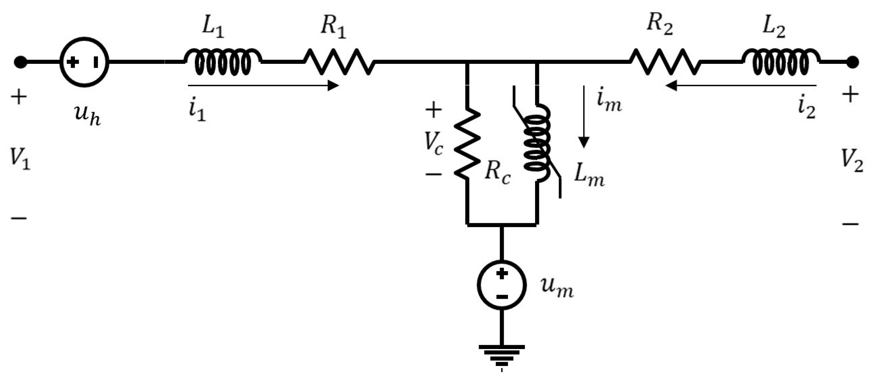
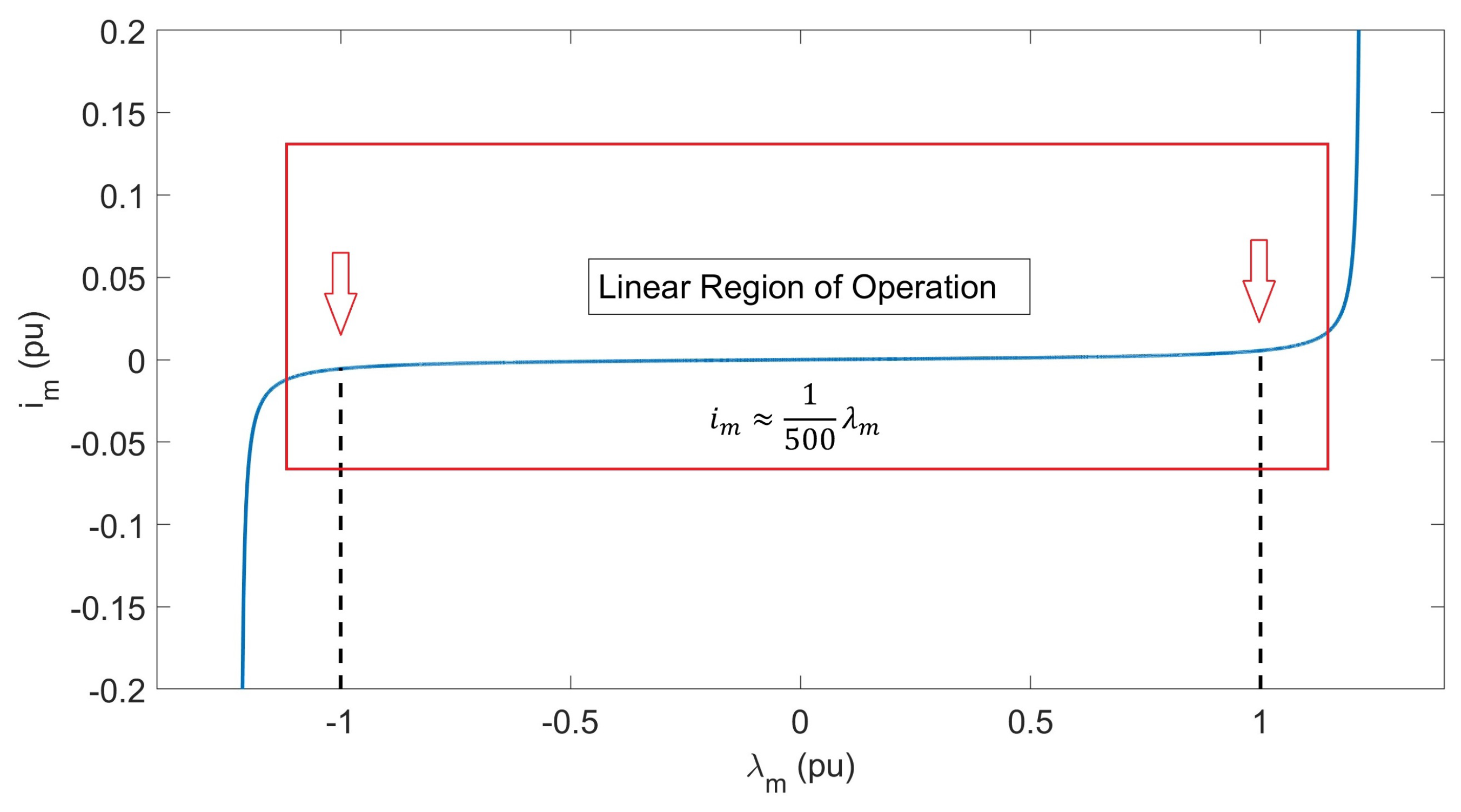
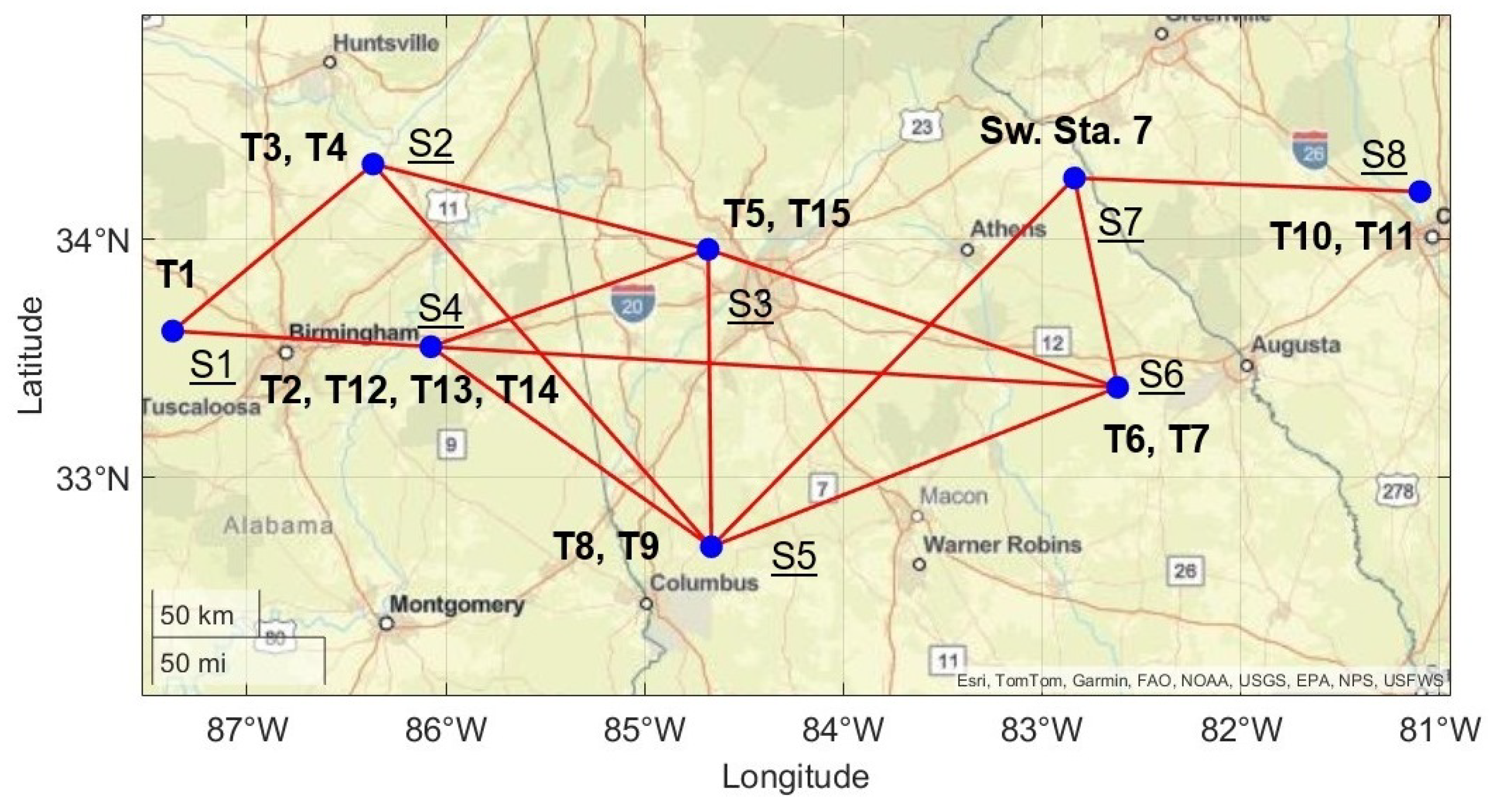
2.2. Horton et al. 20-Bus System

The model used in this paper is a dynamic version of the Horton et al. model [28]. The Horton et al. system model comprises 8 substations with 15 transformers and 15 transmission lines [29]. In this paper, a per-phase transformer model is used to represent the transformers in the system. The schematic of the per-phase transformer is shown in Figure 3. $R_1$ and $R_2$ are winding resistances, $L_1$ and $L_2$ are winding inductances, $R_C$ models the core losses, and $L_m$ is the linearized core inductance. The primary, secondary, and magnetizing path currents are $i_1$, $i_2$, and $i_m$, respectively. The corresponding system of equations for Figure 3 is given in (4), where $u_m$ is a neutral path control term and $u_h$ is a transmission line control term.

$$\left[\begin{array}{c}{L}_1{\dot{i}}_1\\ L_2{\dot{i}}_2\\ {\dot{\lambda }}_m\end{array}\right]=\left[\begin{array}{ccc}-(R_1+R_c)& -R_c& 0\\ -R_c& -(R_2+R_c)& 0\\ R_c& R_c& 0\end{array}\right]\left[\begin{array}{c}{i}_1\\ i_2\\ {\lambda }_m\end{array}\right]+\left[\begin{array}{cc}-1& -1\\ -1& 0\\ 0& 0\end{array}\right]\left[\begin{array}{c}{u}_m\\ u_h\end{array}\right]+\left[\begin{array}{c}{v}_1-R_c{i}_m\\ v_2-R_c{i}_m\\ -R_c{i}_m\end{array}\right]$$

(4)

The full nonlinear equation for $i_m$ is given in [30]. The approximation of Corzine et al.’s characterization of $i_m$ is given as

$$i_m=k_{1}tan(k_2{\lambda }_m),$$

(5)

where $k_1$ and $k_2$ are best fit parameters given as $k_1=0.0016$ and $k_2=1.2879$ [8]. This approximation is shown in Figure 4. However, the systems are specifically tuned such that transformer cores do not saturate when the controllers are applied. Therefore, the system behaves linearly. For the region within the linearized (unsaturated) region, the ratio between $i_m$ and ${\lambda }_m$ is approximately $1/500$, implying that $L_m=500H$ in this simulation. This linear operating region is highlighted in the red box shown in Figure 4. Controllers in the paper are designed to avoid saturation of the transformer magnetic cores. Operation in the saturated region over an extended period of time causes significant losses in power transmission efficiency and produces thermal stresses on the grid due to an excess flow in current [31,32].

The configuration of the Horton et al. model is shown in Figure 5. The labels on the map correspond to the transformer numbers. That is, $T1$ is the first transformer, $T2$ the second, and so on. Sw. Sta. 7 is a switching station that houses no transformers. Substations are labeled with S followed by their corresponding number. Transmission lines are modeled using the $\pi$ transmission line model [33].

3. Controller Design

An active controller paradigm is utilized for HEMP mitigation. There are two types of controller placements that will be explored in this paper. The first is the neutral blocking active device. This is an actively controlled voltage source that is placed along the neutral path of a transformer before it reaches the ground (see Figure 3, $u_m$). The second type of controller placement is the line blocking placement. This consists of an in-series voltage supply along a transmission line (see Figure 3, $u_h$). The controllers are further split into two more subdivisions. The first is the global control scheme wherein full-state knowledge is given to all controllers in the system. The second is the local control scheme wherein only a subset of information is given to the controller. In the case of the neutral blocking controller, the controller will only know the states of the transformer to which it is attached. In the case of the line blocking device, the controller will only read the current passing through the transmission line.

The control law used in this paper is the linear quadratic regulator (LQR). As long as the system acts within the linear regime, the LQR is an optimal controller when trading off between state error and control effort. It is important to note how the LQR is optimal. Minimizing control effort does not necessarily minimize the power flow and stored energy required. Global LQR gains are determined using the linear dynamic model. With this, the feedback control effort is given by

$$u=-K_{lqr}x.$$

(6)

For the local neutral blocking controller, the feedback gains are found by breaking the system down such that the state vector may be described as

$$x^T=\left[\begin{array}{ccc}{x}_{tx}^T& |& x_{ln}^T\end{array}\right],$$

(7)

where $x_{tx}^T$ is the set of states associated with the dynamics of the transformers of the system and $x_{ln}^T$ is the set of states associated with the dynamics of the transmission lines. The transformer dynamics can be further broken down into the n transformer subsystems (in the case of the Horton et al. model, $n=15$).

$${\dot{x}}_{tx}=\left[\begin{array}{c}{\dot{x}}_{tx,1}\\ {\dot{x}}_{tx,2}\\ ⋮\\ {\dot{x}}_{tx,n}\end{array}\right]=\left[\begin{array}{cccc}{A}_1& 0& \dots & 0\\ 0& A_2& \dots & 0\\ ⋮& ⋮& \ddots & ⋮\\ 0& 0& \dots & A_n\end{array}\right]\left[\begin{array}{c}{x}_{tx,1}\\ x_{tx,2}\\ ⋮\\ x_{tx,n}\end{array}\right]+\left[\begin{array}{cccc}{B}_1& 0& \dots & 0\\ 0& B_2& \dots & 0\\ ⋮& ⋮& \ddots & ⋮\\ 0& 0& \dots & B_n\end{array}\right]\left[\begin{array}{c}{u}_1\\ u_2\\ ⋮\\ u_n\end{array}\right]$$

(8)

Feedback gains are calculated using full-state knowledge of subsystems in the grid. That is, the feedback control effort for the controller on the i-th transformer is given by

$$u_i=-K_{1\times 3}{x}_{tx,i}.$$

(9)

If the controller as the i-th transformer is excluded from the placement solution, $u_i(t)=0\forall t$.

Alternatively, the controllers may be placed in-series with the transmission lines. The dynamics for the local LQR formulation are then given as

$${\dot{x}}_{ln}=\left[\begin{array}{c}{\dot{x}}_{ln,1}\\ {\dot{x}}_{ln,2}\\ ⋮\\ {\dot{x}}_{ln,n}\end{array}\right]=\left[\begin{array}{cccc}{A}_1& 0& \dots & 0\\ 0& A_2& \dots & 0\\ ⋮& ⋮& \ddots & ⋮\\ 0& 0& \dots & A_n\end{array}\right]\left[\begin{array}{c}{x}_{ln,1}\\ x_{ln,2}\\ ⋮\\ x_{ln,n}\end{array}\right]+\left[\begin{array}{cccc}{B}_1& 0& \dots & 0\\ 0& B_2& \dots & 0\\ ⋮& ⋮& \ddots & ⋮\\ 0& 0& \dots & B_n\end{array}\right]\left[\begin{array}{c}{u}_1\\ u_2\\ ⋮\\ u_n\end{array}\right].$$

(10)

In (10), $x_{ln,i}$ is the current through the i-th transmission line of the system. The system has a total of n transmission lines. This leads to the feedback law

$$u_i=-K_{1\times 1}{x}_{ln,i}.$$

(11)

If the controller at the i-th transmission line is excluded from the placement solution, $u_i(t)=0\forall t$.

Active controllers are used in lieu of neutral blocking caps, despite the traditional use of passive controllers [34,35]. Neutral capacitors are commonly stated to be the “optimal” method to mitigate the impact of low-frequency HEMP insults on the power grid [9,11,36]. For low-frequency insults that appear as or nearly as DC ($<<$60 Hz), blocking capacitors have approximately infinite impedance and effectively act as open circuits. High-frequency signals (≥60 Hz) pass through the blocking capacitors with little impedance. However there are several issues that arise from the utilization of capacitors as blocking devices.

Recall the per-phase transformer model shown in Figure 3. This system is a first-order dissipative system, and, as such, any impulse (such as the early portion of the $E_{3A}$ domain of the HEMP insult) will decay exponentially over time [37]. Adding a capacitor to the system increases the order of the system from one to two [38]. While the new second-order system is dissipative, it is now also oscillatory (i.e., the system rings) [8,37]. The additional oscillatory dynamics negatively impacts power quality of the system [39,40].

Raising the order of the transformer system also implies that the capacitors do not inherently dissipate energy. Instead, capacitors will move power around the power grid to be dissipated off through resistive elements. From a first-principal approach, EMP mitigation should remove excess energy from the insult while ensuring that sensitive power grid equipment is protected. Blocking capacitors are integrators that increase the order of system without removing energy from it. For these reasons, actively controlled integral controllers are also not considered for HEMP mitigation.

The LQR may be considered an optimally tuned linear PID controller [41,42]. Argelaguet et al. show that PID controllers may be tuned utilizing the LQR optimization process [41]. It has been shown that, following the LQR optimization process, PID gains may be determined to generate fast system response times with minimal overshoot. Likewise, Silva and Erraz show that an LQR-based procedure may be applied to tuning PID controllers for unconstrained Lagrangian systems [42]. The passive capacitor solution may be thought of as an improperly tuned PID controller [8].

Furthermore, capacitors have been shown to degrade significantly over time and become prone to failure in high-voltage use cases [43,44]. A series of factors may lead to the degradation of capacitors. The primary factor appears to be temperature, according to Zhou and Blaabjerg [43]. High temperatures lead to the breakdown of dielectric material, leading to the inability of the capacitor to store the appropriate amount of energy at the desired voltages. Additional factors may include, but are not limited to, general aging, leading to the breakdown of dielectric material, and high-voltage surges, akin to those present in the higher-frequency portions of the HEMP insult. For these reasons, this paper will not examine the conventional use of capacitors when laying out system requirements.

4. Controllability

4.1. Background

From Ogata, “A system is said to be controllable at time $t_0$ if it is possible by means of an unconstrained control vector to transfer the system from any initial state $x(t_0)$ to any other state in a finite interval of time.” [45]. That is, given an unbounded control effort from an actuator, the system may be driven from one state to any other state over a finite amount of time. The concept of controllability is best understood as a mapping between an input to an arbitrary (desired) system output. Suppose that there exist two arbitrary vector fields, $\overrightarrow{f}(x)\in {\mathbb{R}}^n$ and $\overrightarrow{g}(x)\in {\mathbb{R}}^m$, where n is the number of system states and m is the number of system inputs. There then may (or may not) exist a third vector field, $\overrightarrow{\mathcal{F}}(x)$, generated by the Lie bracket of $\overrightarrow{f}(x)$ and $\overrightarrow{g}(x)$ that takes an input $\overrightarrow{g}(x)=\overrightarrow{u}\in {\mathbb{R}}^m$, defines an embedding in ${\mathbb{R}}^n$, and maps the input of the system to the output [46]. In control theory, this mapping is presented as the controllability matrix. The generalized controllability mapping is given as

$$\mathcal{C}=\left[\begin{array}{ccccc}\overrightarrow{g}& (a{d}_{\overrightarrow{f}}^1,\overrightarrow{g})& (a{d}_{\overrightarrow{f}}^2,\overrightarrow{g})& \dots & (a{d}_{\overrightarrow{f}}^n-1,\overrightarrow{g})\end{array}\right],$$

(12)

where

$$\begin{array}{cc}\hfill (a{d}_{\overrightarrow{f}}^1,\overrightarrow{g})& =[\overrightarrow{f},\overrightarrow{g}]={\displaystyle \frac{\partial \overrightarrow{g}}{\partial \overrightarrow{x}}}\overrightarrow{f}-{\displaystyle \frac{\partial \overrightarrow{f}}{\partial x}}\overrightarrow{g}\hfill \\ \hfill (a{d}_{\overrightarrow{f}}^2,\overrightarrow{g})& =[\overrightarrow{f},[\overrightarrow{f},\overrightarrow{g}]]={\displaystyle \frac{\partial (a{d}_{\overrightarrow{f}}^1,g)}{\partial \overrightarrow{x}}}\overrightarrow{f}-{\displaystyle \frac{\partial \overrightarrow{f}}{\partial \overrightarrow{x}}}(a{d}_{\overrightarrow{f}}^1,g)\hfill \\ \hfill (a{d}_{\overrightarrow{f}}^3,\overrightarrow{g})& =[\overrightarrow{f},[\overrightarrow{f},[\overrightarrow{f},\overrightarrow{g}]]]={\displaystyle \frac{\partial (a{d}_{\overrightarrow{f}}^2,\overrightarrow{g})}{\partial \overrightarrow{x}}}\overrightarrow{f}-{\displaystyle \frac{\partial \overrightarrow{f}}{\partial \overrightarrow{x}}}(a{d}_{\overrightarrow{f}}^2,\overrightarrow{g})\hfill \\ \hfill & ⋮\hfill \\ \hfill (a{d}_{\overrightarrow{f}}^n,\overrightarrow{g})& =[\overrightarrow{f},(a{d}_{\overrightarrow{f}}^{n-1},\overrightarrow{g})].\hfill \end{array}$$

(13)

The system is stated to be controllable if and only if the expression in (12) does not lose rank. If this mapping does not lose rank, then the system may be driven from any arbitrary starting state to any arbitrary final state over a finite period of time [47].

The aforementioned controllability analysis may be more familiar in the linear case. Suppose that a linear system’s dynamics are given as

$$\dot{x}(t)=Ax+Bu,$$

(14)

where A is the dynamics matrix, B is the control matrix, u is the control vector, and x is the state vector of the system. As such, the controllability matrix from (12) simplifies to

$$\mathcal{C}=\left[\begin{array}{cccc}B& AB& \dots & A^{n-1}B\end{array}\right],$$

(15)

where n is the total number of states in the system. If the matrix in (15) is of rank $<n$, then the system presented in (14) is not globally controllable. The concept of mapping through the controllability matrix may be further elucidated with the help of the Cayley–Hamilton theorem [48]. For the sake of simplicity (but not for the loss of generality), suppose that a system is linear with only one input, $u(t)$, given by (14). The mapping that goes from the input to the system states is simply

$$\mathcal{C}\left[\begin{array}{c}u(t)\\ \dot{u}(t)\\ ⋮\\ u^{(n-1)}(t)\end{array}\right]=\left[\begin{array}{c}\dot{x}(t)\\ \ddot{x}(t)\\ ⋮\\ x^{(n)}(t)\end{array}\right]-\left[\begin{array}{c}A\\ A^2\\ ⋮\\ A^{(n)}\end{array}\right]A^{n}x(t),$$

(16)

where $\mathcal{C}$ is the controllability mapping, previously defined in (12) and (15).

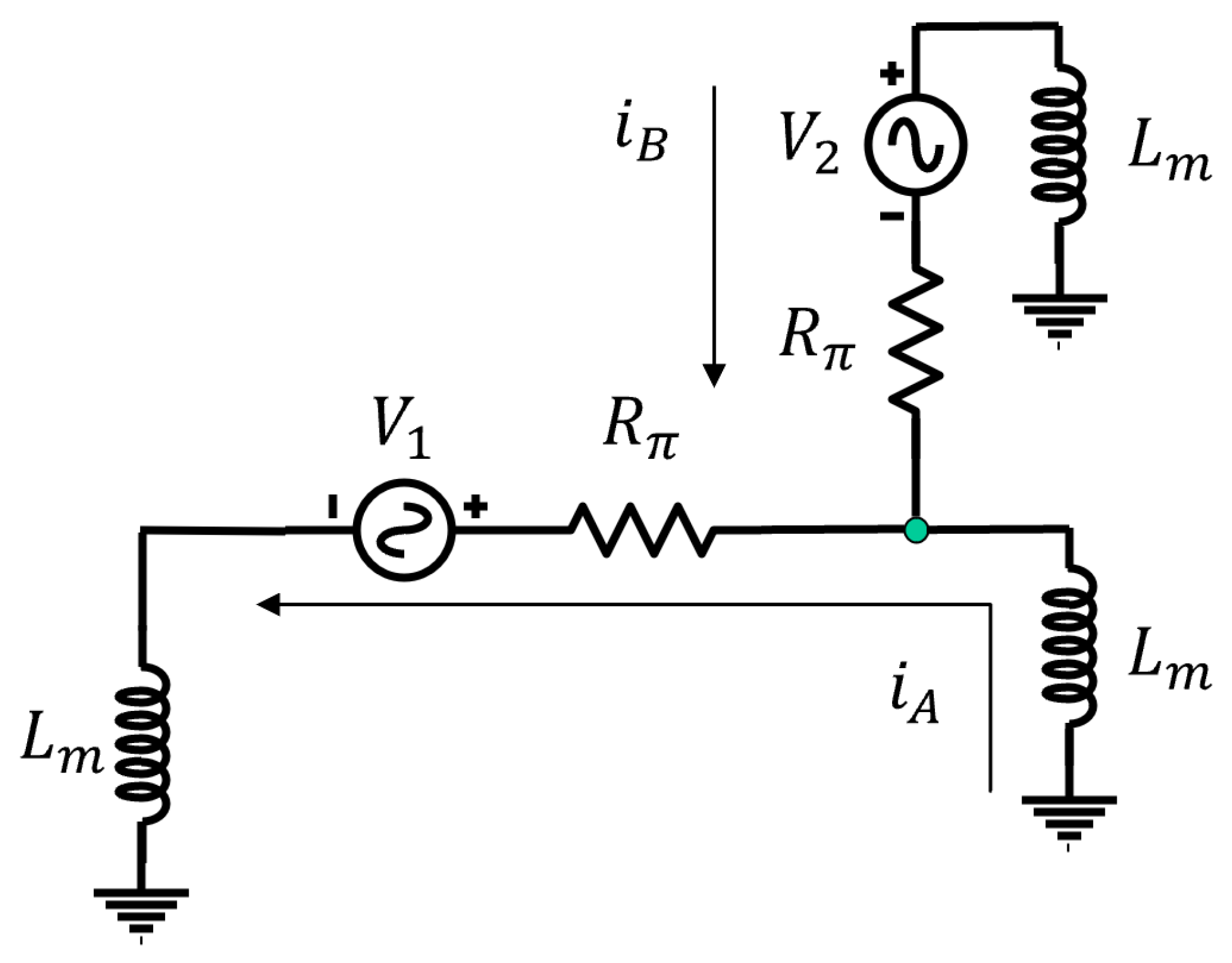
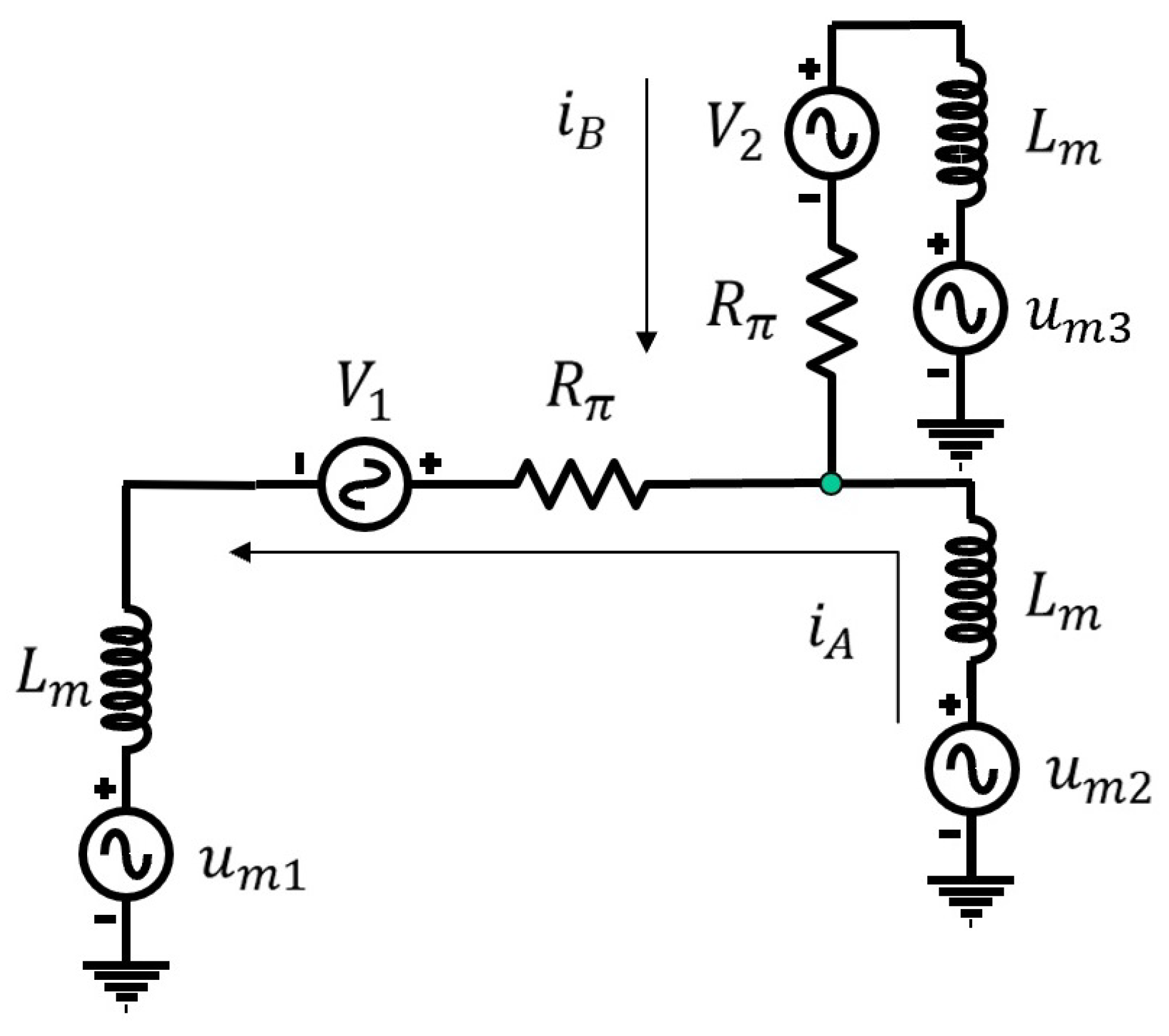
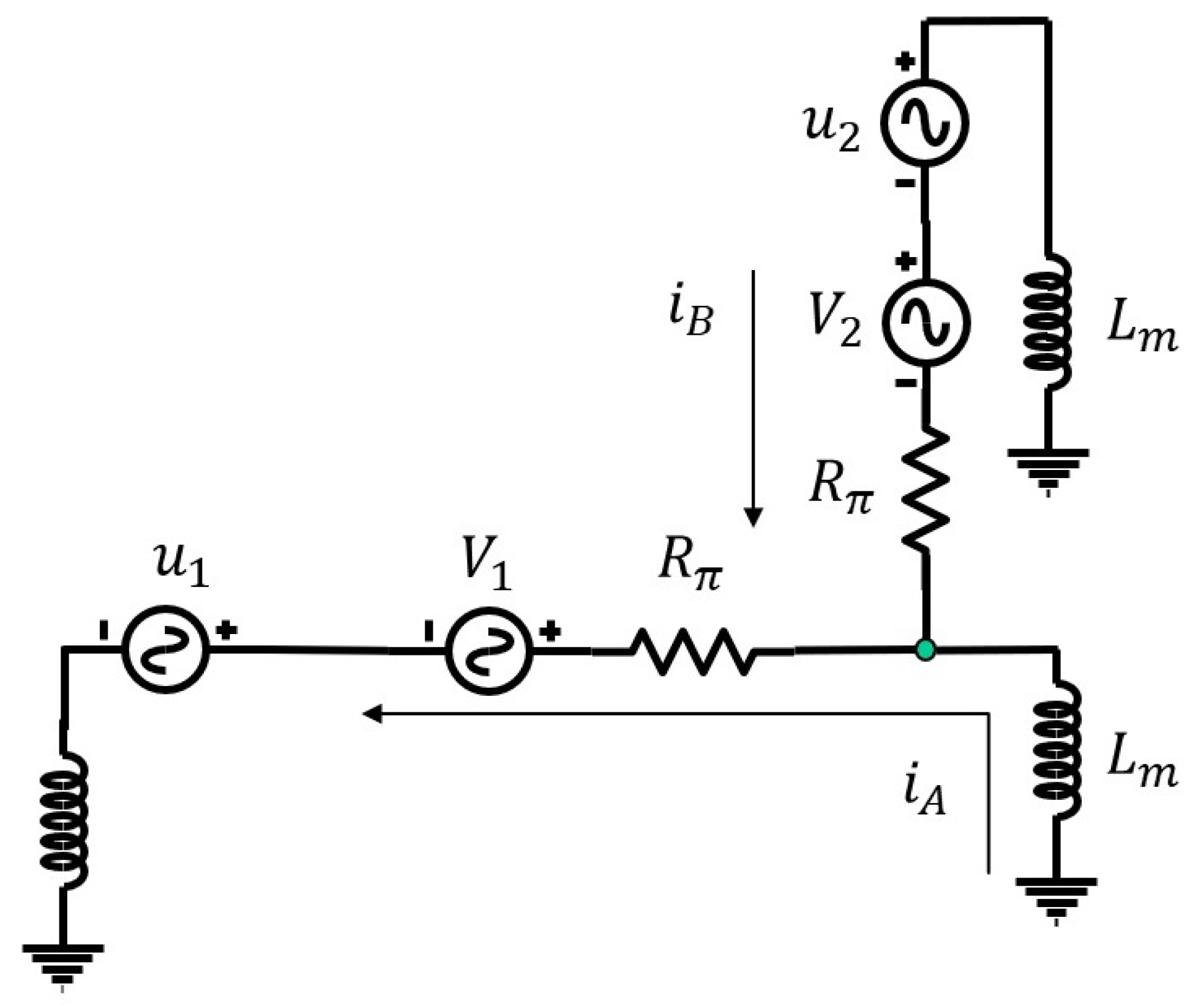
4.2. The Disturbance Influence Problem

Conventionally, controllability analysis provides information on whether or not it is possible to reach all states in a system from any arbitrary states given a finite time period using a controller or actuator of some sorts. Indeed, some work has been carried out in power grid analysis from the classical perspective of controllability analysis [15,49]. However, there is still information left to be gleaned by exploiting the definition of controllability. A system may be controllable from the perspective of an externally occurring event, such as an HEMP insult. Consider the simplified 3-bus system from Donnelly et al. [49]. This simplified system is considered for the sake of computational power and memory without the loss of generality. A schematic of the simplified system is shown in Figure 6.

Transformers are treated as inductors and the transmission lines are treated as purely resistive elements. Additionally, the HEMP insult is treated as two arbitrary voltage sources, $V_1$ and $V_2$, on the transmission lines. These assumptions are made as the HEMP insult presented in this paper is of sufficiently low frequency to appear as a (near, but not quite) DC signal. Correspondingly, the state equations that describe the system are given as

$$\begin{array}{cc}\hfill \dot{x}& =\left[\begin{array}{cc}-{\displaystyle \frac{2R_{\pi }}{3L_m}}& -{\displaystyle \frac{R_{\pi }}{3L_m}}\\ -{\displaystyle \frac{R_{\pi }}{3L_m}}& -{\displaystyle \frac{2R_{\pi }}{3L_m}}\end{array}\right]x+\left[\begin{array}{cc}{\displaystyle \frac{2}{3L_m}}& {\displaystyle \frac{1}{3L_m}}\\ -{\displaystyle \frac{1}{3L_m}}& -{\displaystyle \frac{2}{3L_m}}\end{array}\right]\left[\begin{array}{c}{V}_1\\ V_2\end{array}\right]\hfill \\ \hfill & =Ax+D^{T}V,\hfill \end{array}$$

(17)

where $R_{\pi }$ is the resistance of the transmission line and $L_m$ is the simplified inductance of the transformers. The disturbance influence problem examines how a disturbance, such as an HEMP insult, is mapped to the states of the system. As such, the disturbance influence controllability matrix is given as

$$\mathcal{C}=\left[\begin{array}{cc}{D}^T& A{D}^T\end{array}\right].$$

(18)

In order to remove all influence of an HEMP signal from a power grid, (18) must lose rank. For this analysis, it will be assumed that active controllers will be tuned such that they are able to open the circuit where they are placed. The controllers are placed in series with the transmission lines and provide a controlled voltage to mitigate the insult. The exact nature of the controllers is irrelevant to this analysis for the time being. For the system shown in Figure 6 with no mitigation devices, the controllability matrix comes to

$$\mathcal{C}=\left[\begin{array}{cccc}{\displaystyle \frac{2}{3L_m}}& {\displaystyle \frac{1}{3L_m}}& -{\displaystyle \frac{R_{\pi }}{3L_m^2}}& 0\\ -{\displaystyle \frac{1}{3L_m}}& -{\displaystyle \frac{2}{3L_m}}& 0& {\displaystyle \frac{R_{\pi }}{3L_m^2}}\end{array}\right].$$

(19)

The rank of (19) is 2. Consequently, the GIC is capable of controlling all states of the entire system. Therefore, mitigation devices must be placed throughout the system to lessen the impact of the HEMP insult. In Figure 7, $u_{hi}$ is the i-th transmission line blocking device and $u_{mi}$ is the i-th neutral blocking device. Suppose that a mitigation device, $u_{h1}$, is placed along the horizontal transmission line to remove the influence of $V_1$ on the system by blocking one of the paths to ground, as shown in Figure 7. The controllability matrix becomes

$$\mathcal{C}=\left[\begin{array}{cc}{\displaystyle \frac{1}{3L_m}}& 0\\ -{\displaystyle \frac{2}{3L_m}}& {\displaystyle \frac{R_{\pi }}{3L_m^2}}\end{array}\right].$$

(20)

The rank of (20) is also 2. Once again, this means that the GIC insult is capable of controlling all system states. It is not sufficient only to place a mitigation device along the horizontal transmission line (i.e., only $u_{h1}$). Similarly, the controllability matrix becomes

$$\mathcal{C}=\left[\begin{array}{cc}{\displaystyle \frac{2}{3L_m}}& -{\displaystyle \frac{R_{\pi }}{3L_m^2}}\\ -{\displaystyle \frac{1}{3L_m}}& 0\end{array}\right]$$

(21)

when $V_2$ is blocked with only one mitigation device, $u_{h2}$ (once again, by blocking a path to ground), as shown in Figure 7. The rank of (21) is also 2. The only case in which controllability is lost is when mitigation devices, $u_{h1}$ and $u_{h2}$, are placed in series along both transmission lines.

Similarly, mitigation devices may be placed along the neutral path of transformers. If only one mitigation device, $u_{m3}$, is placed between the top right transformer, as shown in Figure 7, and the ground, then there will exist one loop through the circuit to the ground from the bottom left and bottom right transformers. Likewise, if only one mitigation device is placed between the transformer on the bottom left, $u_{m1}$, or bottom right, $u_{m2}$, as in Figure 7, and its respective ground, then there will still remain one loop through the common ground from the top transformer to the unprotected bottom transformer.

Therefore, if protecting a power grid using transmission line blocking devices, all m transmission lines must have some form of mitigation to minimize influence from an HEMP insult. Alternatively, if protecting a power grid using neutral blocking devices, then $n-1$ transformer neutral paths must be blocked to minimize influence from an HEMP insult. That is, all loops through the power grid through the ground must be eliminated in some manner. However, there are two conditions which suggest that an HEMP signal will not have full system controllability. Firstly, an HEMP signal is a bounded input. That is, over the finite time period that an HEMP signal is transmitted through the power grid, the HEMP signal will only exert a finite amount of effort (voltage or current) across the power grid. Secondly, the grid’s states do not have to be driven to a specific desired final state. It is permissible to operate transformers and transmission lines within some range of state values. For instance, the transformers presented in this paper need only to be kept within an unsaturated region of operation, so any value of magnetic core flux between $-1.2$ pu and $1.2$ pu is deemed acceptable. Therefore, it is possible that there exists a subset of mitigation device placements that does not block all paths through ground such that the power grid remains within desired bounds.

5. Observability

5.1. Background

The observability of a system dictates the ability to map a set of system outputs to the true states of the system [47]. If a system is observable, then it is possible to ascertain the initial conditions of the system and estimate states of the system. That is, if a system is deemed observable, then an observer (i.e., state estimator) may be constructed to determine full-state knowledge of the system. Concomitantly, there is at least one asymptotically stable filter for the observable system [50]. Suppose that there exists some general system (linear or nonlinear) given by the equations

$$\dot{x}(t)=f(x)$$

(22a)

$$y(x)=h(x)$$

(22b)

where $x(t)$ is the vector of system states, $f(x)$ is the dynamics vector of the system, $h(x)$ is the system measurement vector, and $y(x)$ is the system output vector. If the system in (22) is observable, then it is possible to determine the exact states of the system using an observer.

General observability is determined by first taking the 0^th through ${(n-1)}^{th}$ Lie derivatives of the system outputs along the vector field $f(x)$, where n is the total number of states in the system.

$$\begin{array}{cc}\hfill {\pounds }_f^0& =y(x)\hfill \\ \hfill {\pounds }_f^1& =\nabla y(x)·f(x)\hfill \\ \hfill & ⋮\hfill \\ \hfill {\pounds }_f^i& ={\displaystyle \frac{\partial }{\partial x}}\left\{{\pounds }_f^{i-1}(y(x))\right\}·f(x)\hfill \\ \hfill & ⋮\hfill \\ \hfill {\pounds }_f^{n-1}& ={\displaystyle \frac{\partial }{\partial x}}\left\{{\pounds }_f^{n-2}(y(x))\right\}·f(x)\hfill \end{array}$$

(23)

The Lie derivatives of (23) are then formed into the differential embedding map, $\Phi$ [47].

$$\Phi =\left[\begin{array}{c}{\pounds }_f^0\\ {\pounds }_f^1\\ ⋮\\ {\pounds }_f^i\\ ⋮\\ {\pounds }_f^{n-1}\end{array}\right]$$

(24)

The observability matrix is then given as the Jacobian of the mapping $\Phi$,

$$\mathcal{O}={\displaystyle \frac{\partial \Phi }{\partial x}}.$$

(25)

Observability may be more familiar to the reader in the linear form. Suppose there exists some linear system

$${\displaystyle \frac{dx(t)}{dt}}=Ax(t)$$

(26a)

$$y(t)=Cx(t)$$

(26b)

where $x(t)$ is the vector of system states, A is the dynamics matrix, $y(t)$ is the system output vector, and C is the system measurement matrix. The matrix $\mathcal{O}$ simplifies to

$$\mathcal{O}=\left[\begin{array}{c}C\\ CA\\ ⋮\\ C{A}^i\\ ⋮\\ C{A}^{n-1}\end{array}\right].$$

(27)

If the rank of $\mathcal{O}$ is equal to the number of states in the system, then the system is said to be observable, and full-state knowledge may be determined using an observer with the given system measurements.

5.2. Observability of a Power Grid

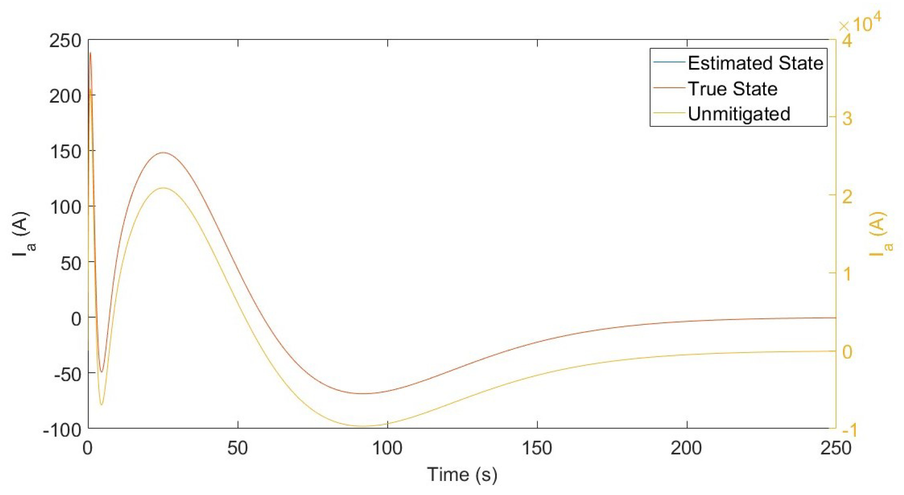
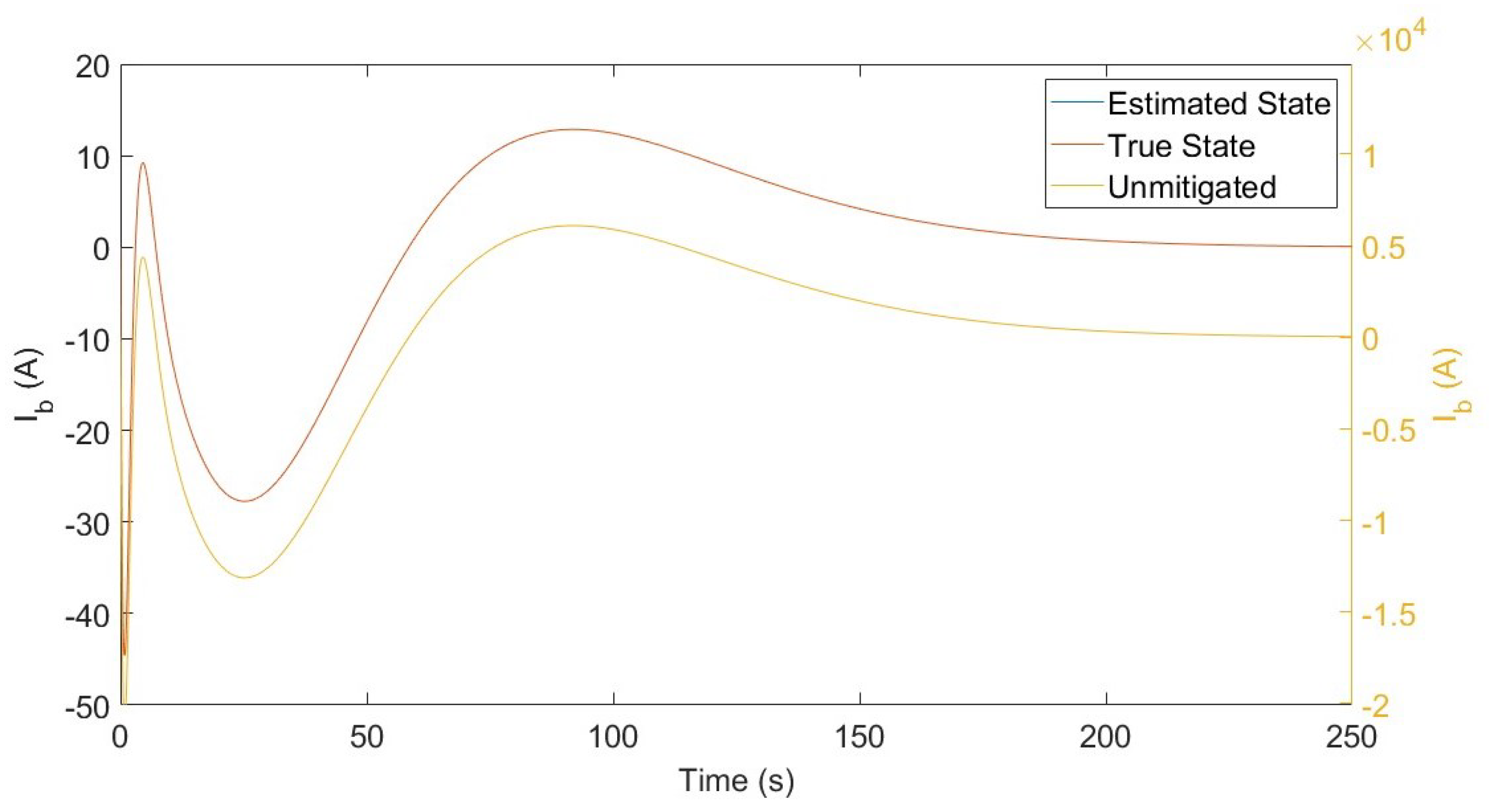
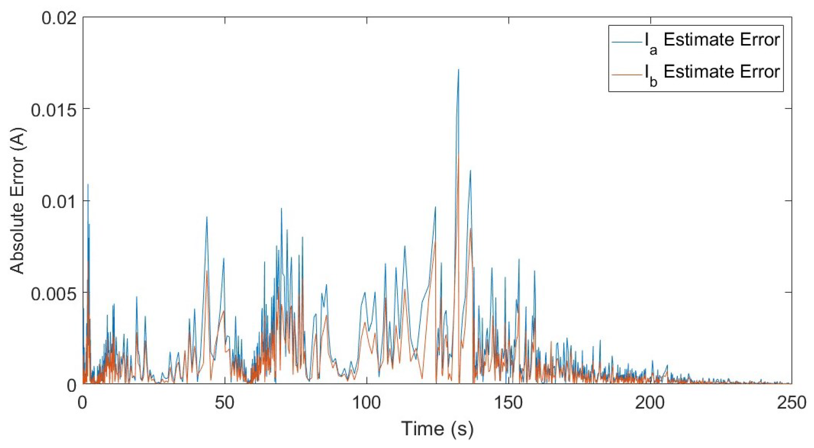
Recall the simplified 3-bus power grid model shown in Figure 6. Suppose now that only one sensor is placed in the system to detect $i_A$. The measured state output of the system is then given by

$$y(t)=\left[\begin{array}{cc}1& 0\end{array}\right]x(t).$$

(28)

From (27), the measurement mapping (from measured state to true state) is then

$$\mathcal{O}=\left[\begin{array}{cc}1& 0\\ -{\displaystyle \frac{2R_{\pi }}{3L_m}}& -{\displaystyle \frac{R_{\pi }}{3L_m}}\end{array}\right].$$

(29)

The rank of (29) is 2, meaning that the system is observable with only one sensor. To demonstrate how this works, an observer is constructed for a global control scheme. Actively controlled energy storage devices are placed in series with the two transmission lines in the model, as shown in Figure 8. A Kalman filter is utilized as the observer [51]. Given a set of Kalman gains, L, and LQR feedback gains, K, the estimated dynamics of the system are shown in (30).

$$\begin{array}{cc}\hfill \dot{\widehat{x}}& =(A-LC-BK)\widehat{x}+Ly\hfill \\ \hfill y& =Cx\hfill \end{array}$$

(30)

The results of the state observer-LQR controller are shown in Figure 9, Figure 10 and Figure 11. The error is low enough is the estimated and true states that the two are almost entirely overlapped.

When expanding the observability analysis to the Horton et al. model, it was found that only one state is required to be measured to ensure observability. It did not matter which state was measured as every combination of only one measured state produced an observable system. This comes with the strict requirement that the system plant must be known exactly. This means that, as long as one state is being measured somewhere on the grid and the system plant is known, system states can be estimated using an observer. This is due to the highly coupled nature of the grid. The same mechanisms that allow energy to freely flow through the system (recall the disturbance influence controllability analysis) also allow a high level of information flow.

There are some issues with using only one sensor to estimate full-state information. This creates a single point of failure within the system. If that sensor is removed or disabled, then measurements can no longer be made. Additional caution must be taken with the implementation of an observer for power grid management. The observer gains of the Kalman filter require knowledge of the state space of the entire power grid. Portions of the power grid may fail during an HEMP attack, so the observer gains may not provide sufficient estimations of the states. Additionally, errors in system knowledge will lead to sub-optimal observer gains. Degraded equipment may deviate from the true system plant from what has been fed to the Kalman filter, also leading to sub-optimal observer gains. However, the Kalman filter does prove to be highly beneficial when dealing with noisy signals and error in sensor reading. Additionally, more sensors with periodical communication may be added into the system to update the Kalman filter, similar to GPS-navigation systems.

6. Results

The results presented in this section were produced by simulations in Matlab and were gathered by applying an HEMP insult to the Horton et al. [29] model and per-phase transformer models, previously mentioned in this paper. The HEMP signal, regardless of power grid topology, does not need to be entirely blocked in order to meet system specifications. This conclusion is reached through exploitation of the definition of controllability. The HEMP signal is a bounded input, so, right away, it cannot be said that any grid is truly globally controllable using the HEMP as an input signal. Additionally, the state vector of any grid does not need to be driven to any one state. Rather, the state of the power grid must be driven to some state wherein all transformers do not saturate. As such, there is an infinite set of possible states that satisfy this requirement, as long as all ${\lambda }_m$ values remain within $-1.2$ pu and $1.2$ pu.

This is demonstrated on the aforementioned Horton et al. 20-bus model in Figure 5 [29]. The bounding cases suggest a very strict criterion of blocking all transmission lines for the transmission line blocking case or blocking all but one neutral path for the neutral blocking case. However, the HEMP signal input is bounded and the system does not need to be driven to one specific state. It will be shown in this section that only a subset of grid assets needs to be protected in order to ensure acceptable levels of HEMP mitigation.

6.1. All Permutations Neutral Blocking Case

Presented in this subsection is a collection of the worst-case ${\lambda }_m$ in pu across all transformers in a grid exposed to an HEMP insult angled from 0 to $31\pi /16$. That is, the HEMP signal is oriented in every possible direction in $\pi /16$ increments. The grid is protected by placing an active controller along the neutral path of the transformers. The all permutations neutral case looks at every possible permutation of neutral blocking device placement combinations. There are a total of $2^{15}$ different possible combinations of neutral blocking device placements. The first set of data looked at is the global neutral controller case. The global neutral controller is able to act with full state knowledge of the system.

Table 1. Best case protection for a global neutral blocking control scheme.

# of Controllers	Transformer Number															Max. |${\mathit{\lambda }}_{\mathit{m}}$| (pu)
	1	2	3	4	5	6	7	8	9	10	11	12	13	14	15
8	X	X	X	X				X	X			X	X			1.1053
9	X	X	X	X	X						X	X	X		X	0.6580
10	X	X	X	X	X	X	X					X	X		X	0.6414
11	X	X	X	X	X	X	X			X		X	X		X	0.5990
12	X	X	X	X	X	X	X	X			X	X	X		X	0.5785
13	X	X	X	X	X	X	X	X	X		X	X	X		X	0.4948
14	X	X	X	X	X	X	X	X	X	X	X	X	X		X	0.5015
15	X	X	X	X	X	X	X	X	X	X	X	X	X	X	X	0.5228

shows the maximum $|{\lambda }_m|$ across all transformers for various best-case configurations using the neutral blocking global LQR control scheme. An “X” under a transformer number denotes that a controller has been placed at that transformer’s neutral path to the ground.

With the global neutral control scheme, there are a total of 193 placement combinations that do not allow transformer saturation out of the 32,768 possible controller placement possibilities. with the minimum required number of global neutral controllers being 8. The local neutral control scheme prevents information flow between controllers (similar to blocking capacitors). This effectively means that a controller on the neutral path of transformer i is only capable of reading out the states of transformer i.

Table 2. Best-case protection for a local neutral blocking control scheme.

# of Controllers	Transformer Number															Max. |${\mathit{\lambda }}_{\mathit{m}}$| (pu)
	1	2	3	4	5	6	7	8	9	10	11	12	13	14	15
9	X	X	X	X	X						X	X	X		X	0.4234
10	X	X	X	X	X	X	X					X	X		X	0.3890
11	X	X	X	X	X	X	X			X		X	X		X	0.3890
12	X	X	X	X	X	X	X	X			X	X	X		X	0.3618
13	X	X	X	X	X	X	X	X	X		X	X	X		X	0.3346
14	X	X	X	X	X	X	X	X	X	X	X	X	X		X	0.3346
15	X	X	X	X	X	X	X	X	X	X	X	X	X	X	X	0.5233

shows the maximum $|{\lambda }_m|$ across all transformers for various best-case configurations using the neutral blocking local LQR control scheme. An “X” under a transformer number denotes that a controller has been placed at that transformer’s neutral path to the ground.

In the local neutral blocking case, there are a total of 324 placement combinations that do not allow transformer saturation out of the 32,768 total possible placement combinations. It took a minimum of nine local neutral controllers to ensure grid protection.

6.2. All Permutations Transmission Line Blocking Case

Presented in this subsection is a collection of the worst-case ${\lambda }_m$ in pu across all transformers in a grid exposed to an HEMP insult angled from 0 to $31\pi /16$. That is, the HEMP signal is oriented in every possible direction in $\pi /16$ increments. The all permutations transmission line blocking case looks at every possible permutation of transmission line blocking device placement combinations. There are a total of $2^{15}$ different possible combinations of transmission line blocking device placements. The first set of data looked at is the global transmission line case. The global transmission line controller is able to act with full state knowledge of the system.

Table 3. Best-case protection for a global transmission line control scheme.

# of Controllers	Transmission Line (Subst. to Subst.)															Max. |${\mathit{\lambda }}_{\mathit{m}}$| (pu)
	2→3	2→5	2→1	1→4	3→5	3→6	3→6	3→4	4→5	4→5	4→6	5→6	5→7	6→7	7→8
3			X	X							X					0.9342
4		X		X				X			X					0.5528
5		X	X	X			X	X								0.4375
6		X	X	X			X	X							X	0.3427
7	X		X	X		X				X	X				X	0.3204
8	X		X	X		X		X	X		X				X	0.3117
9	X	X	X	X		X	X	X			X				X	0.3051
10	X	X	X	X		X	X	X		X	X				X	0.3010
11	X	X	X	X		X	X	X	X		X		X		X	0.2971
12	X	X	X	X		X	X	X	X	X	X	X			X	0.2947
13	X	X	X	X		X	X	X	X	X	X	X	X		X	0.2920
14	X	X	X	X		X	X	X	X	X	X	X	X	X	X	0.2918
15	X	X	X	X	X	X	X	X	X	X	X	X	X	X	X	0.2918

shows the maximum $|{\lambda }_m|$ across all transformers for various best-case configurations using the transmission line blocking global LQR control scheme. An “X” in a column denotes that a controller has been placed along a transmission line that spans from substation $n\to m$. For the global transmission line blocking controller, there are a total of 18,834 combinations of placements that did not permit a single transformer to saturate. The minimum required number of global transmission line controllers to prevent saturation is three.

Table 4. Best-case protection for a local transmission line control scheme.

# of Controllers	Transmission Line (Subst. to Subst.)															Max. Flux (pu)
	2→3	2→5	2→1	1→4	3→5	3→6	3→6	3→4	4→5	4→5	4→6	5→6	5→7	6→7	7→8
11	X	X	X	X	X	X	X	X	X	X	X					1.0755
12	X	X	X	X	X	X	X	X	X	X	X		X			1.0713
13	X	X	X	X	X	X	X	X	X	X	X	X	X			1.0587
14	X	X	X	X	X	X	X	X	X	X	X	X	X		X	1.0535
15	X	X	X	X	X	X	X	X	X	X	X	X	X	X	X	1.0535

shows the maximum $|{\lambda }_m|$ across all transformers for various best-case configurations using the transmission line blocking local LQR control scheme. An “X” in a column denotes that a controller has been placed along a transmission line that spans from substation $n\to m$. For the local transmission line blocking controller, there is a total of 135 combinations of placements that did not permit a single transformer to saturate. The minimum required number of local transmission line controllers to prevent transformer core saturation is 11.

6.3. Discussion of Results

It has been shown in this paper that fewer than 14 neutral and 15 transmission line controllers are required to protect the power grid from an HEMP insult. This is in line with the prior statement on controllability and how the HEMP disturbance does not meet the strict requirements for controllability. There are two notable phenomena present in the results. The first is that there is a discernible difference in the total number of required controllers between the global and local transmission line blocking cases. The second is that the neutral controller shows little difference between local and global controls.

The transmission line blocking methods rely more heavily on the presence of information (or lack thereof). A global control scheme is capable of generating destructive interference with its voltage effort to draw power away from transformers and transmission lines. The local controller, however, is only capable of removing power from the line that it is attached to. Therefore, one solution of removing power from the controller’s locality is to push power off into neighboring transformers and transmission lines. This action may or may not produce constructive or destructive interference.

The reason for the consistency in performance across both neutral blocking cases is the same reason for the inconsistency in performance across both transmission line blocking cases. Information flow is less important for the neutral blocking cases. The neutral blocking devices are less able to push power around the system than the transmission line blocking devices, and so information is less important to the neutral blocking devices. If the transmission line blocking devices are capable of global communications, they are able to cooperate and more readily remove the disturbances. Disturbance rejection is easier to perform when the controller (actuator) is placed more closely to the disturbance (or poorly behaved) portion of the system [52].

7. Conclusions

This paper began with a formal definition of controllability. Unlike conventional controllability analysis, this paper presents a novel use of controllability to determine how influential an HEMP insult is on the grid. For a generic unbounded insult, the power grid is only protected once all returns through the ground have been severed in one way or another. This may come in the form of protecting all transmission lines or all but one neutral paths in the power grid. However, this definition of controllability is stricter than required. An HEMP insult will be bounded over finite time and, thus, the grid is never truly globally controllable from the perspective of an HEMP input. Additionally, the grid has an “acceptable” collection of states in which it may reside (i.e., all ${\lambda }_m$ are not required to be zeroed out, just within the unsaturated region of operation). This suggests that only a subset of the grid needs to be protected to ensure HEMP mitigation. Indeed, as few as 3 transmission line blocking controllers are required for the full protection of the 15 transformer power grid presented in this paper.

The analysis continues with an observability study of the power grid and generates a minimum sensor requirement for full-state estimation. It was shown that, provided the system plant is known in its entirety, an observer on the power grid needs only one sensor to estimate the states of the system. This is due to the ability for high amounts of information to flow through the system. In practice, a single sensor is less than ideal in terms of redundancy as it creates a single point of failure for the entire system estimator. Additionally, as the Kalman filter requires full knowledge of the state space, any failure on any portion of the grid will alter the accuracy of the observer. Future observer implementation will require updates based on the health status of the power grid.

The conclusions presented in this paper only act as initial guidance in the design of a control system for the mitigation of an HEMP insult on a power grid. The all-permutation results show the minimum required number of controllers to mitigate an HEMP insult on the power grid, but they do not explain the physics of the system or why these controller placements are deemed optimal. This set of results will be used as a baseline case for future optimization work. Further work will need to be carried out on an algorithm for the determination of optimal controller placement. Furthermore, other control laws are yet to be explored and they may influence optimal controller placement.

References

1. Foster, R.A.; Frickey, S.J. Strategies, Protections and Mitigations for Electric Grid from Electromagnetic Pulse Effects; Technical Report; Idaho National Lab (INL): Idaho Falls, ID, USA, 2016.
2. Baker, G.H. Electromagnetic Pulse Resilience of United States Critical Infrastructure: Progress and Prognostics. J. Crit. Infrastruct. Policy 2021, 2, 35–46. [Google Scholar] [CrossRef]
3. SRI International. Starfish Prime, Santitized Version. 1962. Available online: https://apps.dtic.mil/sti/citations/ADA955694 (accessed on 15 May 2025).
4. Vittitoe, C.N. Did High-Altitude EMP Cause the Hawaiian Streetlight Incident. System Design and Assessment Notes. 1989. Available online: https://ece-research.unm.edu/summa/notes/SDAN/0031.pdf (accessed on 15 May 2025).
5. Barnes, A.K.; Mate, A.; Bent, R. A Review of the GIC Blocker Placement Problem. In Proceedings of the 2024 IEEE/IAS 60th Industrial and Commercial Power Systems Technical Conference (I&CPS), Las Vegas, NV, USA, 19–23 May 2024; pp. 1–6. [Google Scholar]
6. Etemadi, A.H.; Rezaei-Zare, A. Optimal placement of GIC blocking devices for geomagnetic disturbance mitigation. IEEE Trans. Power Syst. 2014, 29, 2753–2762. [Google Scholar] [CrossRef]
7. Liang, Y.; He, D.; Zhu, H.; Chen, D. Optimal blocking device placement for geomagnetic disturbance mitigation. IEEE Trans. Power Deliv. 2019, 34, 2219–2231. [Google Scholar] [CrossRef]
8. Donnelly, T.J.; Wilson, D.G.; Robinett, R.D.; Weaver, W.W. Top-Down Control Design Strategy for Electric Power Grid EMP (E3) Protection. In Proceedings of the 2023 IEEE Texas Power and Energy Conference (TPEC), College Station, TX, USA, 13–14 February 2023; pp. 1–6. [Google Scholar] [CrossRef]
9. Wang, D.; Li, Y.; Dehghanian, P.; Wang, S. Power Grid Resilience to Electromagnetic Pulse (EMP) Disturbances: A Literature Review. In Proceedings of the 2019 North American Power Symposium (NAPS), Wichita, KS, USA, 13–15 October 2019; pp. 1–6. [Google Scholar] [CrossRef]
10. Kappenman, J. Low-Frequency Protection Concepts for the Electric Power Grid: Geomagnetically Induced Current (GIC) and E3 HEMP Mitigation; Metatech Corporation, FERC: Goleta, CA, USA, 2010. [Google Scholar]
11. Tarditi, A.G.; Besnoff, J.S.; Duckworth, R.C.; Li, F.R.; Li, Z.; Liu, Y.; Mcconnell, B.W.; Olsen, R.G.; Poole, B.R.; Piesciorovsky, E.C.; et al. High-Voltage Modeling and Testing of Transformer, Line Interface Devices, and Bulk System Components Under Electromagnetic Pulse, Geomagnetic Disturbance, and Other Abnormal Transients; ORNL/TM-2019/1143; Oak Ridge National Laboratory (ORNL): Oak Ridge, TN, USA, 2019.
12. Garrett, R.; Guttromson, R. A Survey of Preventive and Remediating Mitigations for High-Altitude Electromagnetic Pulse Impacts on the United States Electric Power Grid; Technical report; Sandia National Lab. (SNL-NM): Albuquerque, NM, USA, 2021.
13. Kappenman, J.; Norr, S.R.; Sweezy, G.; Carlson, D.; Albertson, V.; Harder, J.; Damsky, B. GIC mitigation: A neutral blocking/bypass device to prevent the flow of GIC in power systems. IEEE Trans. Power Deliv. 1991, 6, 1271–1281. [Google Scholar] [CrossRef]
14. Zhang, S.M.; Liu, L.G. A mitigation method based on the principle of GIC-even distribution in whole power grids. IEEE Access 2020, 8, 65096–65103. [Google Scholar] [CrossRef]
15. Lehman, C.A.; Donnelly, T.J.; Robinett, R.D., III; Weaver, W.W.; Wilson, D.G. Decoupled, decentralized, lqr-based controls for e3 hemp/gmd mitigation on the power grid. In Proceedings of the Annual Conference of the IEEE Industrial Electronics Society (IECON), Chicago, IL, USA, 3–6 November 2024. [Google Scholar]
16. Lehman, C.A.; Robinett, R.D.; Weaver, W.W.; Wilson, D.G. Solid State Transformer Controls for Mitigation of E3a High-Altitude Electromagnetic Pulse Insults. Energies 2025, 18, 1055. [Google Scholar] [CrossRef]
17. Bhela, S.; Kekatos, V.; Zhang, L.; Veeramachaneni, S. Enhancing observability in power distribution grids. In Proceedings of the 2017 IEEE International Conference on Acoustics, Speech and Signal Processing (ICASSP), New Orleans, LA, USA, 5–9 March 2017; pp. 4551–4555. [Google Scholar]
18. You, M.; Jiang, J.; Tonello, A.M.; Doukoglou, T.; Sun, H. On statistical power grid observability under communication constraints. IET Smart Grid 2018, 1, 40–47. [Google Scholar] [CrossRef]
19. Ryu, M.; Attia, A.; Barnes, A.; Bent, R.; Leyffer, S.; Mate, A. Heuristic algorithms for placing geomagnetically induced current blocking devices. Electr. Power Syst. Res. 2024, 234, 110645. [Google Scholar] [CrossRef]
20. Zhang, H.; Li, Z.; Xue, Y.; Chang, X.; Su, J.; Wang, P.; Guo, Q.; Sun, H. A stochastic bi-level optimal allocation approach of intelligent buildings considering energy storage sharing services. IEEE Trans. Consum. Electron. 2024, 70, 5142–5153. [Google Scholar] [CrossRef]
21. Zhai, X.; Li, Z.; Li, Z.; Xue, Y.; Chang, X.; Su, J.; Jin, X.; Wang, P.; Sun, H. Risk-averse energy management for integrated electricity and heat systems considering building heating vertical imbalance: An asynchronous decentralized approach. Appl. Energy 2025, 383, 125271. [Google Scholar] [CrossRef]
22. Legro, J.R.; Abi-Samra, N.C.; Crouse, J.C.; Hileman, A.R.; Kruse, V.J.; Taylor, E.R., Jr.; Tesche, F.M. Study to Assess the Effects of High-Altitude Electromagnetic Pulse on Electric Power Systems. Phase I, Final Report; Oak Ridge National Laboratory: Oak Ridge, TN, USA, 1986. [CrossRef]
23. IEC 61000-2-9; Electromagnetic Compatibility (EMC). IEC: Geneva, Switzerland, 1996.
24. Brouillette, D. Physical Characteristics of HEMP Waveform Benchmarks for Use in Assessing Susceptibilities of the Power Grid, Electrical Infrastructures, and Other Critical Infrastructure to HEMP Insults; Department of Energy Memo: Washington, DC, USA, 2021.
25. Lee, R.H.W.; Shetye, K.S.; Birchfield, A.B.; Overbye, T.J. Using detailed ground modeling to evaluate electric grid impacts of late-time high-altitude electromagnetic pulses (E3 HEMP). IEEE Trans. Power Syst. 2018, 34, 1549–1557. [Google Scholar] [CrossRef]
26. Hutchins, T. Modeling, Simulation, and Mitigation of the Impacts of the Late Time (E3) High-Altitude Electromagnetic Pulse on Power Systems. Ph.D. Thesis, University of Illinois at Urbana–Champaign, Champaign, IL, USA, 2015. [Google Scholar]
27. Tesche, F.M.; Barnes, P.R.; Meliopoulos, A.P. Magnetohydrodynamic Electromagnetic Pulse (MHD-EMP) Interaction with Power Transmission and Distribution Systems; Oak Ridge National Laboratory: Oak Ridge, TN, USA, 1992. [CrossRef]
28. Donnelly, T.J.; Wilson, D.G.; Robinett, R.D.; Weaver, W.W. Dynamic Model of a 20-Bus Power System for HEMP/GMD Controls-based Mitigation Design. In Proceedings of the 2023 North American Power Symposium (NAPS), Asheville, NC, USA, 15–17 October 2023; pp. 1–6. [Google Scholar] [CrossRef]
29. Horton, R.; Boteler, D.; Overbye, T.J.; Pirjola, R.; Dugan, R.C. A Test Case for the Calculation of Geomagnetically Induced Currents. IEEE Trans. Power Deliv. 2012, 27, 2368–2373. [Google Scholar] [CrossRef]
30. Corzine, K.; Kuhn, B.; Sudhoff, S.; Hegner, H. An improved method for incorporating magnetic saturation in the q-d synchronous machine model. IEEE Trans. Energy Convers. 1998, 13, 270–275. [Google Scholar] [CrossRef]
31. Dommel, H.; Yan, A.; Wei, S. Harmonics from transformer saturation. IEEE Trans. Power Deliv. 1986, 1, 209–215. [Google Scholar] [CrossRef]
32. Bolduc, L.; Gaudreau, A.; Dutil, A. Saturation time of transformers under dc excitation. Electr. Power Syst. Res. 2000, 56, 95–102. [Google Scholar] [CrossRef]
33. MathWorks. Pi Section Line. Available online: https://www.mathworks.com/help/sps/powersys/ref/pisectionline.html (accessed on 5 December 2024).
34. Faxvog, F.; Fuchs, G.; Jensen, W.; Wojtczak, D.; Marz, M.; Dahman, S. HV power transformer neutral blocking device (NBD) operating experience in Wisconsin. In Proceedings of the MIPSYCON Conference November, St. Paul, MN, USA, 7–9 November 2017; Volume 7. [Google Scholar]
35. Nazir, M.; Burkes, K.; Enslin, J.H. Electrical safety considerations of neutral blocker placements for mitigating DC. IEEE Trans. Ind. Appl. 2020, 57, 1113–1121. [Google Scholar] [CrossRef]
36. Horton, R. Magnetohydrodynamic Electromagnetic Pulse Assessment of the Continental US Electric Grid; Electric Power Research Institute: Palo Alto, CA, USA, 2017. [Google Scholar]
37. Nise, N.S. Control Systems Engineering, 7th ed.; Wiley: Hoboken, NJ, USA, 2015; pp. 157–235. [Google Scholar]
38. Robinett, R.D., III; Wilson, D.G. Nonlinear Power Flow Control Design; Springer: Berlin/Heidelberg, Germany, 2011. [Google Scholar]
39. Baggini, A. Handbook of Power Quality; JohnWiley & Sons, Ltd.: Hoboken, NJ, USA, 2008. [Google Scholar]
40. Lehman, C.A.; Robinett, R.D.; Weaver, W.W.; Wilson, D.G. Hamiltonian-Based Power Flow and Stability Analysis on a Passively Controlled Multi-Frequency Power System. In Proceedings of the 2024 International Symposium on Power Electronics, Electrical Drives, Automation and Motion (SPEEDAM), Napoli, Italy, 19–21 June 2024; pp. 242–247. [Google Scholar] [CrossRef]
41. Argelaguet, R.; Pons, M.; Quevedo, J.; Aguilar, J. A New Tuning of PID Controllers Based on LQR Optimization. Ifac Proc. Vol. 2000, 33, 271–276. [Google Scholar] [CrossRef]
42. Silva, E.I.; Erraz, D.A. An LQR Based MIMO PID Controller Synthesis Method for Unconstrained Lagrangian Mechanical Systems. In Proceedings of the 45th IEEE Conference on Decision and Control, San Diego, CA, USA, 13–15 December 2006; pp. 6593–6598. [Google Scholar] [CrossRef]
43. Zhou, D.; Blaabjerg, F. Reliability evaluation of power capacitors in a wind turbine system. In Proceedings of the 2018 IEEE Applied Power Electronics Conference and Exposition (APEC), San Antonio, TX, USA, 4–8 March 2018; pp. 3264–3269. [Google Scholar] [CrossRef]
44. Rezaei, M.A.; Fathollahi, A.; Akbari, E.; Saki, M.; Khorgami, E.; Teimouri, A.R.; Chronopoulos, A.T.; Mosavi, A. Reliability Calculation Improvement of Electrolytic Capacitor Banks Used in Energy Storage Applications Based on Internal Capacitor Faults and Degradation. IEEE Access 2024, 12, 13146–13164. [Google Scholar] [CrossRef]
45. Ogata, K. Modern Control Engineering, 5th ed.; Prentice Hall: Hoboken, NJ, USA, 2010. [Google Scholar]
46. Haynes, G.W.; Hermes, H. Nonlinear Controllability via Lie Theory. Siam J. Control 1970, 8, 450–460. [Google Scholar] [CrossRef]
47. Whalen, A.J.; Brennan, S.N.; Sauer, T.D.; Schiff, S.J. Observability and Controllability of Nonlinear Networks: The Role of Symmetry. Phys. Rev. X 2015, 5, 011005. [Google Scholar] [CrossRef]
48. Jacobson, N. Lectures in Abstract Algebra; D. Van Nostrand Company, Inc.: New York, NY, USA, 1953. [Google Scholar]
49. Donnelly, T.J.; Wilson, D.G.; Robinett, R.D.; Weaver, W.W. Control Strategies for Large Power Transformer HEMP/GMD Protection. In Proceedings of the 2023 North American Power Symposium (NAPS), Asheville, NC, USA, 15–17 October 2023; pp. 1–6. [Google Scholar] [CrossRef]
50. Van Handel, R. Observability and nonlinear filtering. Probab. Theory Relat. Fields 2009, 145, 35–74. [Google Scholar] [CrossRef]
51. Kalman, R.E. A New Approach to Linear Filtering and Prediction Problems. Trans. ASME—J. Basic Eng. 1960, 82, 35–45. [Google Scholar] [CrossRef]
52. Morris, K.; Yang, S. Comparison of actuator placement criteria for control of structures. J. Sound Vib. 2015, 353, 1–18. [Google Scholar] [CrossRef]
Figure 1. Magnitude of the E 3 A portion of an HEMP insult [24].
Energies 18 02614 g001
Figure 2. Magnitude of the E 3 B portion of an HEMP insult [24].
Energies 18 02614 g002
Figure 3. Per-phase transformer model with a neutral and transmission line blocking device.
Energies 18 02614 g003
Figure 4. Tangent approximation of the i m curve given by Corzine et al., with the linear region of operation/unsaturated regime denoted [8,30].
Energies 18 02614 g004
Figure 5. Map of the Horton et al. model with transformers labeled [29].
Energies 18 02614 g005
Figure 6. Depiction of the 3-bus simplified model to elucidate disturbance influence controls.
Energies 18 02614 g006
Figure 7. Grid with the transmission lines and paths to neutral blocked.
Energies 18 02614 g007
Figure 8. Power grid system with blocking devices u h 1 and u h 2 along both transmission lines.
Energies 18 02614 g008
Figure 9. Comparison of the estimated i a , the true i a , and the unmitigated true i a states. The estimated and true states are effectively overlaid, as estimation error is near zero.
Energies 18 02614 g009
Figure 10. Comparison of the estimated i b , the true i b , and the unmitigated true i b states. The estimated and true states are effectively overlaid, as estimation error is near zero.
Energies 18 02614 g010
Figure 11. Error over time from the state estimator and true states.
Energies 18 02614 g011