Optimization of Energy Use for Zero-Carbon Buildings Considering Intraday Source-Load Uncertainties

Abstract

Building operational energy consumption accounts for a significant share of global energy consumption, and it is crucial to promote renewable energy self-sufficiency and operational optimization for zero-carbon buildings. However, scheduling strategies relying on day-ahead forecasts have limitations, and ignoring the ambiguity of short-term source-load forecasts is prone to the risk of scheduling failures. To address this issue, this study proposes an intraday optimization method for zero-carbon buildings under the source-load fuzzy space, which innovatively constructs a fuzzy chance constraint model of Photovoltaic (PV) output and load demand, enforces energy self-sufficiency as a constraint, and establishes a multi-objective optimization framework with thermal comfort as the main objective and power adjustment balance as the sub-objective, so as to quantify the decision risk through intraday energy optimization. Experiments show that the proposed method quantifies the decision-maker’s risk preference through fuzzy opportunity constraints, balances conservatism and aggressive strategies, and improves thermal comfort while safeguarding energy independence, providing a risk-controllable scheduling paradigm for the decarbonized operation of buildings.

1. Introduction

As of 2024, China’s existing building stock has exceeded 70 billion square meters, with the construction sector emitting 5.31 billion tons of CO₂ equivalent annually, accounting for 48.3% of the nation’s energy-related carbon emissions [1]. These figures underscore the strategic priority of energy conservation and decarbonization in the building sector to advance China’s carbon reduction goals [2]. Zero-carbon buildings, which fully leverage renewable energy to meet annual energy demands and achieve carbon neutrality through advanced energy management systems, have gained global recognition. Internationally, this concept has catalyzed policy-driven initiatives and industrial practices aiming at sustainable development.

Ensuring the secure and stable operation of zero-carbon buildings without grid dependency necessitates a paradigm shift from traditional energy consumption to self-sufficient operation. While effective operational energy management is critical for this transition, maintaining energy autonomy during actual operation presents persistent technical challenges.

First, significant temporal volatility exists between local renewable energy generation and electricity demand [3], with fluctuations exhibiting distinct characteristics across different time scales. Current research on energy system management primarily adopts a day-ahead-to-intraday perspective. For instance, a carbon trading-integrated day-ahead scheduling model was proposed in [4] to minimize both carbon emissions and operational costs, where power-to-heat conversion and battery energy storage are employed during intraday phases to mitigate wind power forecasting errors. Reference [5] proposes a day-ahead–intraday optimization model for zero-carbon energy systems combining seasonal hydrogen storage and battery storage, achieving zero-carbon, economic, and high-efficiency operation in isolated high-renewable systems. Reference [6] introduces a carbon-constrained day-ahead–intraday optimal scheduling method, which accounts for dynamic carbon trading intervals, carbon quotas, and green certificate trading coefficients across multiple time scales, further reducing system-wide emissions. However, these studies rigidly follow day-ahead plans during intraday phases without dynamically adapting scheduling strategies to real-time variations, prioritizing system stability over flexibility.

Second, the operational management of zero-carbon buildings faces uncertainties. Influenced by natural conditions and external factors, intraday short-term forecasts for renewable generation and load demand exhibit inherent fuzziness [7]. Ignoring such fuzziness in energy optimization risks operational failures. Existing approaches for addressing source-load uncertainties include multi-scenario analysis, robust optimization, and fuzzy chance-constrained programming (FCCP). Multi-scenario methods construct representative scenario sets to balance optimization outcomes across diverse conditions [8], yet their computational intensity and prolonged solving times [9] limit applicability to longer-term scheduling. Robust optimization ensures feasibility under worst-case scenarios [10] but suffers from excessive conservatism, leading to the underutilization of resources [11]. In contrast, FCCP models uncertainties within fuzzy domains [12], enabling the flexible adjustment of robustness via confidence levels while maintaining computational efficiency.

Reference [13] employs a K-means-based scenario generation method to create typical day-ahead and intraday renewable energy output uncertainty scenarios. Stochastic optimization is subsequently applied to derive renewable energy supplier bidding strategies. References [14,15] utilize Monte Carlo simulation to generate multiple probabilistic source-load scenarios, enabling the stochastic optimization of energy management systems under renewable and load uncertainties, thereby enhancing system flexibility. Reference [16] proposes an adjustable robust optimization method to address the conservatism of traditional robust approaches. However, its worst-case scenarios rely on historical datasets, limiting applicability to unseen extreme conditions. Reference [17] integrates FCCP to handle wind power and load demand uncertainties while resolving multi-objective weight allocation via an improved analytic hierarchy process. Reference [18] introduces a credibility theory-based Integrated Energy Service Provider (IESP) robust fuzzy trading strategy, balancing economic efficiency and robustness to mitigate the over-conservatism of conventional robust optimization. The comparison of the three uncertainty treatment methods is shown in

Table 1. Comparison of uncertainty handling methods.

Method	Uncertainty Characterization	Computational Time	Conservatism
Robust Optimization	Bounded worst-case scenarios	Moderate	High
Stochastic Programming	Discrete probabilistic scenarios	Long	Low
Monte Carlo Simulation	Statistical sampling of scenarios	Very long	Scenario-dependent
Proposed FCCP	Fuzzy membership functions	Short	Adjustable

.

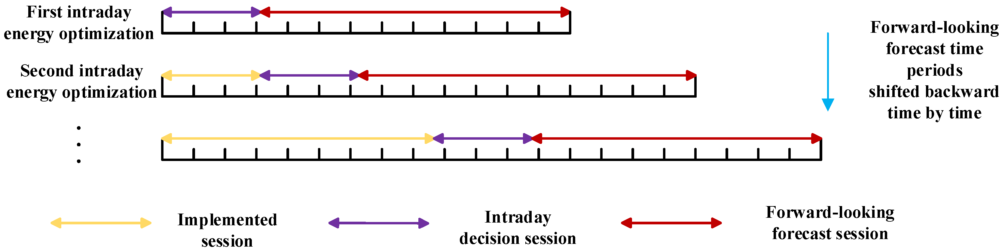
This paper proposes an intraday energy optimization method for zero-carbon buildings under fuzzy source-load uncertainties. First, intraday short-term PV output and load demand are modeled within a fuzzy space, establishing fuzzy chance constraints based on source-load uncertainties. To further enhance indoor thermal comfort, the proposed model enforces energy self-sufficiency as a hard constraint, prioritizes thermal comfort as the primary objective, and balances power adjustment equilibrium as a secondary objective. A goal programming approach holistically addresses these multi-objective trade-offs. FCCP quantifies decision risks, ensuring that energy dispatch plans satisfy constraints with a predefined confidence level. Finally, a forward-looking intraday optimization framework dynamically refines energy dispatch decisions across daily time slots, improving operational feasibility.

2. Zero-Carbon Building Model Construction

This section establishes the mathematical foundation for zero-carbon building operation by developing three core component models: renewable energy generation, energy conversion/storage systems, and flexible resources. The modeling framework specifically addresses the operational characteristics of PV systems under cloud occlusion uncertainty, heat transfer dynamics of heating, ventilation, and air conditioning (HVAC) systems with thermal storage integration, and bidirectional energy interaction mechanisms of battery-electric vehicle (EV) coordination. These interconnected models collectively form the physical infrastructure for subsequent energy optimization, while explicitly considering the temporal coupling effects between different energy carriers. These models are common in buildings, so the research methodology of this paper is equally applicable in all types of buildings.

2.1. Intraday Uncertainty-Incorporated PV Power Output Modeling

During intraday periods, stochastic factors such as cloud cover significantly impact the output power of PV systems over short timescales. These fluctuations often become critical factors affecting the supply–demand balance in zero-carbon buildings. While short-term cloud shading events lasting tens of minutes are almost impossible to predict in day-ahead stages, they directly compromise the implementation of energy scheduling plans for zero-carbon buildings.

This paper models the intraday PV uncertainty primarily through two parameters, cloud occlusion duration and solar irradiance attenuation ratio, as follows:

$$\left\{\begin{array}{c}{P}_{\mathrm{m}\mathrm{a}\mathrm{x}}^{\mathrm{P}\mathrm{V}}=A_{\mathrm{P}\mathrm{V}}·\sigma ·G_t\\ 0\le P_t^{\mathrm{P}\mathrm{V}}\le P_{\mathrm{m}\mathrm{a}\mathrm{x}}^{\mathrm{P}\mathrm{V}}\end{array}\right.$$

(1)

where $P_t^{\mathrm{P}\mathrm{V}}$ denotes the output power of the residential PV system at time interval $t$; $P_{\mathrm{m}\mathrm{a}\mathrm{x}}^{\mathrm{P}\mathrm{V}}$ is the maximum PV power output; $A_{\mathrm{P}\mathrm{V}}$ represents the area of the solar panel; $\sigma$ is the PV conversion efficiency; and $G_t$ stands for the forecasted solar irradiance at time $t$.

As indicated by Equation (1), the maximum PV output power at each time interval is determined by the solar irradiance level, which is directly influenced by the solar radiation loss ratio. Considering the direct relationship between solar irradiance and these two uncertainty parameters, the short-term PV output model under cloud cover uncertainty is presented in Equations (2) and (3), i.e.,

$$P_t^{\mathrm{P}\mathrm{V}}=A_{\mathrm{P}\mathrm{V}}·\sigma ·G_t$$

(2)

$$G_t=\overline{G_t}-B_t^{\mathrm{P}\mathrm{V}}\eta \overline{G_t}$$

(3)

where $P_t^{\mathrm{P}\mathrm{V}}$ denotes the PV output power (kW); $A_{\mathrm{P}\mathrm{V}}$ represents the rooftop PV panel area (m²); $\sigma$ is the photoelectric conversion efficiency; $G_t$ indicates the actual solar irradiance under uncertainty effects (kW/m²); and $\overline{G_t}$ stands for the predicted solar irradiance value (kW/m²). The parameter $\eta$ quantifies the solar radiation loss ratio due to cloud shading, and $B_t^{\mathrm{P}\mathrm{V}}$ serves as a binary state variable indicating the presence of cloud occlusion phenomena. These two parameters, $B_t^{\mathrm{P}\mathrm{V}}$ and $\eta$, constitute the uncertainty parameters in this scenario, whose uncertainty sets are mathematically defined in Equations (4) and (5).

$$\sum _{t=1}^N{B}_t^{\mathrm{P}\mathrm{V}}\le {\Gamma }_{\mathrm{P}\mathrm{V}}$$

(4)

$$B_t^{\mathrm{P}\mathrm{V}}\in \left\{\mathrm{0,1}\right\},{\Gamma }_{\mathrm{P}\mathrm{V}}\in \left[0,N\right], \eta \in [0,{\eta }_{\mathrm{m}\mathrm{a}\mathrm{x}}]$$

(5)

where the parameter ${\Gamma }_{\mathrm{P}\mathrm{V}}$ controls uncertainty set conservatism by specifying maximum shaded intervals. ${\Gamma }_{\mathrm{P}\mathrm{V}}=0$ yields deterministic optimization using forecasted irradiance (least conservative), while ${\Gamma }_{\mathrm{P}\mathrm{V}}=N$ implements worst-case scenarios (most conservative). ${\eta }_{max}$ defines the maximum cloud-induced radiation loss. Both $N$ and ${\eta }_{\mathrm{m}\mathrm{a}\mathrm{x}}$ are derived from the statistical analysis of historical data on cloud shading events and their impacts.

2.2. Energy Modeling of HVAC Systems Incorporating Hot Water Storage Tanks

HVAC systems are the primary energy-consuming equipment during building operation. This study assumes that the building envelope’s heat dissipation represents the total cooling loss of the building, neglecting additional losses caused by occupant behavior. When the room’s set temperature changes, the air conditioning (AC) system must correspondingly adjust its cooling output. Based on heat transfer principles, the state transition equation for indoor temperature is given by Equation (6), which primarily depends on the change in indoor temperature, the cooling capacity of the AC system, and the building’s cooling dissipation [19]. Dynamic heat transfer in the building envelope under different outdoor conditions is a key component of the cooling load modeling, so the effects of occupant behavior and increased internal heat on building cooling demand are not considered [20].

$$Q_t^{base}=aFK(T_t^{out}-T_t^{in})\Delta t$$

(6)

where $Q_t^{base}$ represents the basic cooling dissipation load of the building envelope (kWh); $a$ is the temperature difference correction coefficient for the building envelope; $F$ is the area of the building envelope (m²); $K$ is the heat transfer coefficient of the building envelope (kW/(m²·°C)); $T_t^{out}$ is the outdoor temperature (°C); and $T_t^{in}$ is the indoor temperature (°C).

When the compressor operates normally, part of the generated thermal power meets the building’s heating demand, while the remaining portion is stored in the hot water storage tank. However, when the compressor stops running, the cooling demand of the building can be met by the stored cooling capacity in the storage tank. Therefore, the cooling balance equation is expressed as Equation (7).

$$Q_t^{\mathrm{c}\mathrm{o}\mathrm{m}}={\eta }^{\mathrm{t}\mathrm{a}\mathrm{n}\mathrm{k}}{Q}_t^{\mathrm{t}\mathrm{a}\mathrm{n}\mathrm{k}}+{\eta }^{\mathrm{A}\mathrm{C}}{Q}_t^{\mathrm{A}\mathrm{C}}$$

(7)

where $Q_t^{\mathrm{t}\mathrm{a}\mathrm{n}\mathrm{k}}$ represents the change in cooling capacity of the heat storage tank (HST) (kWh); $Q_t^{\mathrm{A}\mathrm{C}}$ is the cooling output delivered by the AC system to the indoor space (kWh); $Q_t^{\mathrm{c}\mathrm{o}\mathrm{m}}$ denotes the cooling capacity output by the compressor (kWh); and ${\eta }^{\mathrm{t}\mathrm{a}\mathrm{n}\mathrm{k}}$ and ${\eta }^{\mathrm{A}\mathrm{C}}$ are the heat transfer efficiencies for the portion of cooling stored in the HST and the portion directly delivered to the building, respectively. During compressor shutdown, if the HST does not release stored cooling energy to the building, the AC system’s cooling output becomes zero; conversely, if the HST utilizes its stored cooling capacity to power the system, then $Q_t^{\mathrm{A}\mathrm{C}}>0$ and $Q_t^{\mathrm{t}\mathrm{a}\mathrm{n}\mathrm{k}}<0$, indicating active cooling supply and discharge from the storage tank, respectively.

The HST passively stores energy by utilizing residual heat from chilled water return flow during energy storage mode, while in cooling release mode, it regulates the chilled water flow rate to control cooling output per unit time. The computational model is presented in Equation (8):

$$Q_t^{\mathrm{t}\mathrm{a}\mathrm{n}\mathrm{k}}=\left\{\begin{array}{c}cq(T_t^{\mathrm{H}\mathrm{S}\mathrm{T}}-T_t^{\mathrm{r}\mathrm{e}\mathrm{t}\mathrm{u}\mathrm{r}{\mathrm{n}}_{—}\mathrm{c}\mathrm{h}})\Delta t Q_t^{\mathrm{t}\mathrm{a}\mathrm{n}\mathrm{k}}>0\\ cq(T_t^{\mathrm{r}\mathrm{e}\mathrm{t}\mathrm{u}\mathrm{r}{\mathrm{n}}_{—}\mathrm{d}\mathrm{i}\mathrm{s}}-T_t^{\mathrm{H}\mathrm{S}\mathrm{T}})\Delta t Q_t^{\mathrm{t}\mathrm{a}\mathrm{n}\mathrm{k}}\le 0\end{array}\right.$$

(8)

where $c$ represents the specific heat capacity of water (kWh/(kg·°C)); $q$ is the flow rate of chilled water (kg/h); $T_t^{\mathrm{r}\mathrm{e}\mathrm{t}\mathrm{u}\mathrm{r}{\mathrm{n}}_{—}\mathrm{c}\mathrm{h}}$ and $T_t^{\mathrm{r}\mathrm{e}\mathrm{t}\mathrm{u}\mathrm{r}{\mathrm{n}}_{—}\mathrm{d}\mathrm{i}\mathrm{s}}$ denote the preset return temperatures of chilled water for the HST under its two operating modes, respectively; and $T_t^{\mathrm{H}\mathrm{S}\mathrm{T}}$ indicates the water temperature of the HST, which varies with the charging/discharging of cooling capacity as calculated by Equations (9) and (10).

$$S_{t+1}=S_t+Q_t^{\mathrm{t}\mathrm{a}\mathrm{n}\mathrm{k}}$$

(9)

$$T_t^{\mathrm{H}\mathrm{S}\mathrm{T}}={\displaystyle \frac{S_t}{c\rho V}}$$

(10)

where $S_t$ represents the cooling capacity stored in the HST (kWh); $c$ denotes the specific heat capacity (kWh/(kg·°C)); $\rho$ is the density (kg/m³); and $V$ indicates the water volume in the HST (m³). In cooling mode, since the HST stores energy using residual heat from chilled water return flow, the tank temperature during charging cannot fall below the return water temperature. During discharging, excessively high tank temperatures would reduce the HST’s cooling delivery capacity. Therefore, the tank temperature is subject to both upper and lower bounds:

$$T_{\mathrm{m}\mathrm{i}\mathrm{n}}\le T_t^{\mathrm{H}\mathrm{S}\mathrm{T}}\le T_{\mathrm{m}\mathrm{a}\mathrm{x}}$$

(11)

where $T_{\mathrm{m}\mathrm{i}\mathrm{n}}$ and $T_{\mathrm{m}\mathrm{a}\mathrm{x}}$ represent the minimum and maximum temperature limits (°C) of the HST, respectively, which determine the energy storage capacity of the HST.

The primary energy-consuming components of the HVAC system are the compressor unit and water pumps, whose power consumption must satisfy Equations (12) and (13). When operating in low-energy mode, the system only activates minimal equipment such as water pumps, resulting in a significantly higher coefficient of performance (COP) compared to normal operation conditions.

$$P_t^{\mathrm{A}\mathrm{C}}=P_t^{\mathrm{p}\mathrm{u}\mathrm{m}\mathrm{p}}+P_t^{\mathrm{c}\mathrm{o}\mathrm{m}}$$

(12)

$$P_t^{\mathrm{c}\mathrm{o}\mathrm{m}}\mathrm{C}\mathrm{O}\mathrm{P}\Delta t=Q_t^{\mathrm{c}\mathrm{o}\mathrm{m}}$$

(13)

where $P_t^{\mathrm{A}\mathrm{C}}$ denotes the total electrical power consumption of the system (kW); $P_t^{\mathrm{p}\mathrm{u}\mathrm{m}\mathrm{p}}$ represents the power consumption of water pumps (kW); $P_t^{\mathrm{c}\mathrm{o}\mathrm{m}}$ is the power consumption of the cooling operation (kW); the corresponding cooling output from the compressor unit is represented by $Q_t^{\mathrm{c}\mathrm{o}\mathrm{m}}$ (kWh); and $\mathrm{C}\mathrm{O}\mathrm{P}$ represents the system’s energy efficiency.

Furthermore, the cooling capacity of the AC system is not unlimited and is constrained by both the compressor’s refrigeration power and the operational speed of water pumps. Both the compressor unit and the pump system are subject to maximum power constraints, which must comply with Equation (14).

$$0\le P_t^{\mathrm{c}\mathrm{o}\mathrm{m}}\le P_{\mathrm{m}\mathrm{a}\mathrm{x}}^{\mathrm{c}\mathrm{o}\mathrm{m}}$$

(14)

2.3. Zero-Carbon Building Flexibility Resource Modeling

2.3.1. Modeling of Battery Energy Storage Systems

Battery energy storage systems (BESSs) serve as a critical flexible resource for addressing source-load uncertainty in buildings. Through intraday scheduling, a BESS can effectively mitigate energy mismatches caused by source-load fluctuations. Its operation must comply with the constraints specified in Equations (15)–(18).

$$\begin{array}{c}0\le E_t^{\mathrm{c}\mathrm{h}}\le {\beta }_t{E}_{\mathrm{m}\mathrm{a}\mathrm{x}}^{\mathrm{B}\mathrm{S}}\hfill \\ 0\le E_t^{\mathrm{d}\mathrm{i}\mathrm{s}}\le \left(1-{\beta }_t\right)E_{\mathrm{m}\mathrm{a}\mathrm{x}}^{\mathrm{B}\mathrm{S}}\hfill \end{array}$$

(15)

$$\Delta E_t^{\mathrm{B}\mathrm{S}}=E_t^{\mathrm{c}\mathrm{h}}{\eta }^{\mathrm{c}\mathrm{h}}-E_t^{\mathrm{d}\mathrm{i}\mathrm{s}}/{\eta }^{\mathrm{d}\mathrm{i}\mathrm{s}}$$

(16)

$${\mathrm{S}\mathrm{O}\mathrm{C}}_{t+1}^{\mathrm{B}\mathrm{S}}-{\mathrm{S}\mathrm{O}\mathrm{C}}_t^{\mathrm{B}\mathrm{S}}={\displaystyle \frac{\Delta E_t^{\mathrm{B}\mathrm{S}}}{C_{\mathrm{m}\mathrm{a}\mathrm{x}}^{\mathrm{B}\mathrm{S}}}}$$

(17)

$${\mathrm{S}\mathrm{O}\mathrm{C}}_{\mathrm{m}\mathrm{i}\mathrm{n}}^{\mathrm{B}\mathrm{S}}\le {\mathrm{S}\mathrm{O}\mathrm{C}}_t^{\mathrm{B}\mathrm{S}}\le {\mathrm{S}\mathrm{O}\mathrm{C}}_{\mathrm{m}\mathrm{a}\mathrm{x}}^{\mathrm{B}\mathrm{S}}$$

(18)

where $E_{\mathrm{m}\mathrm{a}\mathrm{x}}^{\mathrm{B}\mathrm{S}}$ is the maximum charge/discharge energy per scheduling period (kWh); ${\beta }_t$ is the binary operating state (1 for charging and 0 for discharging); $\Delta E_t^{\mathrm{B}\mathrm{S}}$ is the net energy change (positive for charging and negative for discharging); ${\eta }^{\mathrm{c}\mathrm{h}}$ and ${\eta }^{\mathrm{d}\mathrm{i}\mathrm{s}}$ are the respective charge/discharge efficiencies; ${\mathrm{S}\mathrm{O}\mathrm{C}}_t^{\mathrm{B}\mathrm{S}}$ is the state of charge (SOC) of the BESS; and ${\mathrm{S}\mathrm{O}\mathrm{C}}_{\mathrm{m}\mathrm{a}\mathrm{x}}^{\mathrm{B}\mathrm{S}}$ and ${\mathrm{S}\mathrm{O}\mathrm{C}}_{\mathrm{m}\mathrm{i}\mathrm{n}}^{\mathrm{B}\mathrm{S}}$ are the upper and lower limits of the BESS’s SOC, respectively, which is used to ensure the safe operation of the BESS.

2.3.2. Modeling of EV

In building energy optimization, EVs serve not only as transportation means but also as crucial flexible resources. Unplanned EV charging behaviors may create significant power demand peaks during specific days or periods, substantially aggravating source-load mismatch in zero-carbon buildings. Therefore, this study develops an intraday time-scale model for EV charging/discharging energy dynamics, as formulated in Equations (19)–(23).

$$E_{i,j}^{\mathrm{E}\mathrm{V}}=E_{i,j}^{\mathrm{E}\mathrm{V}\_\mathrm{c}\mathrm{h}}{\eta }^{\mathrm{E}\mathrm{V}\_\mathrm{c}\mathrm{h}}-E_{i,j}^{\mathrm{E}\mathrm{V}\_\mathrm{d}\mathrm{i}\mathrm{s}}/{\eta }^{\mathrm{E}\mathrm{V}\_\mathrm{d}\mathrm{i}\mathrm{s}}$$

(19)

$$0\le E_{i,j}^{\mathrm{E}\mathrm{V}\_\mathrm{c}\mathrm{h}}\le S_t^{\mathrm{E}\mathrm{V}}{\beta }_t^{\mathrm{E}\mathrm{V}}{E}_{\mathrm{m}\mathrm{a}\mathrm{x}}^{\mathrm{E}\mathrm{V}\_\mathrm{c}\mathrm{h}}$$

(20)

$$0\le E_{i,j}^{\mathrm{E}\mathrm{V}\_\mathrm{d}\mathrm{i}\mathrm{s}}\le S_t^{\mathrm{E}\mathrm{V}}(1-{\beta }_t^{\mathrm{E}\mathrm{V}})E_{\mathrm{m}\mathrm{a}\mathrm{x}}^{\mathrm{E}\mathrm{V}\_\mathrm{d}\mathrm{i}\mathrm{s}}$$

(21)

$${\mathrm{S}\mathrm{O}\mathrm{C}}_{i,t+1}^{\mathrm{E}\mathrm{V}}={\mathrm{S}\mathrm{O}\mathrm{C}}_{i,t}^{\mathrm{E}\mathrm{V}}+{\displaystyle \frac{E_{i,t}^{\mathrm{E}\mathrm{V}}-E_{i,t}^{\mathrm{t}\mathrm{r}\mathrm{i}\mathrm{p}}}{C_{\mathrm{m}\mathrm{a}\mathrm{x}}^{\mathrm{E}\mathrm{V}}}}$$

(22)

$${\mathrm{S}\mathrm{O}\mathrm{C}}_{\mathrm{m}\mathrm{i}\mathrm{n}}^{\mathrm{E}\mathrm{V}}\le {\mathrm{S}\mathrm{O}\mathrm{C}}_{i,t}^{\mathrm{E}\mathrm{V}}\le {\mathrm{S}\mathrm{O}\mathrm{C}}_{\mathrm{m}\mathrm{a}\mathrm{x}}^{\mathrm{E}\mathrm{V}}$$

(23)

where $E_{i,j}^{\mathrm{E}\mathrm{V}\_\mathrm{c}\mathrm{h}}$ represents the energy transferred from the building to the i-th EV during time interval j (kWh); $E_{i,j}^{\mathrm{E}\mathrm{V}\_\mathrm{d}\mathrm{i}\mathrm{s}}$ represents the energy discharged from the i-th EV to the building during time interval $j$ (kWh); ${\eta }^{\mathrm{E}\mathrm{V}\_\mathrm{c}\mathrm{h}}$ and ${\eta }^{\mathrm{E}\mathrm{V}\_\mathrm{d}\mathrm{i}\mathrm{s}}$ represent the energy conversion efficiency during EV charging and discharging, respectively; $E_{\mathrm{m}\mathrm{a}\mathrm{x}}^{\mathrm{E}\mathrm{V}\_\mathrm{c}\mathrm{h}}$ and $E_{\mathrm{m}\mathrm{a}\mathrm{x}}^{\mathrm{E}\mathrm{V}\_\mathrm{d}\mathrm{i}\mathrm{s}}$ are the upper and lower limits of charging and discharging energy per interaction, respectively; ${\beta }_t^{\mathrm{E}\mathrm{V}}$ represents the state variable characterizing the charging/discharging status of the EV during time period $t$, where ${\beta }_t^{\mathrm{E}\mathrm{V}}=1$ indicates that the EV is in charging mode, and ${\beta }_t^{\mathrm{E}\mathrm{V}}=0$ signifies that the EV is engaged in building energy balance regulation through vehicle-to-building (V2B) operation; ${\mathrm{S}\mathrm{O}\mathrm{C}}_{i,t}^{\mathrm{E}\mathrm{V}}$ represents the SOC of the battery in the i-th EV during time period $t$; $E_{i,t}^{\mathrm{t}\mathrm{r}\mathrm{i}\mathrm{p}}$ represents the energy consumed by the i-th EV travelling during time period $t$; $C_{\mathrm{m}\mathrm{a}\mathrm{x}}^{\mathrm{E}\mathrm{V}}$ is the maximum battery capacity of the EV (kWh); and ${\mathrm{S}\mathrm{O}\mathrm{C}}_{\mathrm{m}\mathrm{i}\mathrm{n}}^{\mathrm{E}\mathrm{V}}$ and ${\mathrm{S}\mathrm{O}\mathrm{C}}_{\mathrm{m}\mathrm{a}\mathrm{x}}^{\mathrm{E}\mathrm{V}}$ denote the minimum and maximum allowable SOC for the EV battery, respectively.

3. Multi-Objective Intraday Energy Optimization Based on Goal Programming

This paper constructs a goal programming-based intraday energy optimization model to dynamically adjust the operational decisions of BESSs and EV and AC systems based on intraday short-term source-load forecast data. The model prioritizes indoor thermal comfort as the primary objective, mitigating the conservatism inherent in day-ahead robust decisions by leveraging short-term forecast data. Additionally, it emphasizes the equilibrium of BESS and EV scheduling adjustments to avoid excessive adjustment pressure on any single device, ensuring holistic system efficiency. Furthermore, the model incorporates the fuzziness of source-load forecast data and solves the optimization problem using fuzzy space-based chance-constrained programming. Target planning based on thermal comfort prioritization prioritizes ensuring indoor comfort, both for cooling and heating, so that the regulation strategy can be adapted to different climates.

3.1. Intraday Multi-Objective Optimization Model

Conventional intraday optimization approaches are primarily designed to track day-ahead scheduling plans or align with day-ahead objectives. While day-ahead scheduling ensures secure and stable system operation, building energy management systems often compromise user comfort to some extent. This study reduces day-ahead conservatism via intraday forecasts, prioritizing thermal comfort under energy self-sufficiency constraints. The proposed model improves indoor temperature regulation through dynamic data adjustments while maintaining energy independence from external sources. The objective function is formulated as shown in Equation (24).

$$\mathrm{m}\mathrm{i}\mathrm{n}f=(f_{pm\nu },f_{ba})$$

(24)

where $f_{pm\nu }$ represents the thermal comfort objective for intraday short-term optimization and $f_{ba}$ denotes the equilibrium objective for balancing power adjustments between BESS and EV.

The objective function for indoor thermal comfort $f_{pm\nu }$ is formulated as follows:

$$f_{pmv}={\sum }_{t=1}^T {\delta }_t^{pmv}pm{v}_t$$

(25)

where $f_{pmv}$ denotes the objective function for building thermal comfort and ${\delta }_t^{pmv}$ is the state variable indicating thermal comfort demand.

During intraday short-term optimization, deviations between the predicted source-load results and the day-ahead scenarios imply that the power balance constraints considered in the day-ahead stage are no longer satisfied. Constrained by energy independence requirements, this study can only adjust the charging/discharging power of BESSs and EVs to maintain building power balance, thereby preventing any single device from excessively deviating from the day-ahead scheduling plan and avoiding impacts on SOC states and battery lifespan. Consequently, this issue must be incorporated into the objective function, as specifically formulated below:

$$\mathrm{m}\mathrm{i}\mathrm{n}{f}_{ba}=\mathrm{m}\mathrm{i}\mathrm{n}\mathrm{m}\mathrm{a}\mathrm{x}\left[\begin{array}{cc}{\mathrm{s}}_1\Delta P_{\mathrm{m}\mathrm{a}\mathrm{x}}^{\mathrm{B}\mathrm{E}\mathrm{S}\mathrm{S}}& {,\mathrm{s}}_2\Delta P_{\mathrm{m}\mathrm{a}\mathrm{x}}^{\mathrm{E}\mathrm{V}}\end{array}\right]$$

(26)

$$\mathrm{s}.\mathrm{t}\left\{\begin{array}{c}\Delta P_{\mathrm{m}\mathrm{a}\mathrm{x}}^{\mathrm{B}\mathrm{E}\mathrm{S}\mathrm{S}}=\max [\mid \Delta P_1^{\mathrm{B}\mathrm{E}\mathrm{S}\mathrm{S}}\mid ,\mid \Delta P_2^{\mathrm{B}\mathrm{E}\mathrm{S}\mathrm{S}}\mid ,\dots ,\mid \Delta P_T^{\mathrm{B}\mathrm{E}\mathrm{S}\mathrm{S}}\mid ]\\ \Delta P_{\mathrm{m}\mathrm{a}\mathrm{x}}^{\mathrm{E}\mathrm{V}}=\max [\mid \Delta P_1^{\mathrm{E}\mathrm{V}}\mid ,\mid \Delta P_2^{\mathrm{E}\mathrm{V}}\mid ,\dots ,\mid \Delta P_T^{\mathrm{E}\mathrm{V}}\\ \Delta P_t^{\mathrm{B}\mathrm{E}\mathrm{S}\mathrm{S}}=P_t^{\mathrm{B}\mathrm{E}\mathrm{S}\mathrm{S}}-P_t^{\mathrm{B}\mathrm{E}\mathrm{S}\mathrm{S}\_\mathrm{d}\mathrm{a}}\\ \Delta P_t^{\mathrm{E}\mathrm{V}}=P_t^{\mathrm{E}\mathrm{V}}-P_t^{\mathrm{E}\mathrm{V}\_\mathrm{d}\mathrm{a}}\end{array}\right.$$

(27)

where $f_{ba}$ denotes the objective function for balanced power adjustment; $\Delta P_{\mathrm{m}\mathrm{a}\mathrm{x}}^{\mathrm{B}\mathrm{E}\mathrm{S}\mathrm{S}}$ and $\Delta P_{\mathrm{m}\mathrm{a}\mathrm{x}}^{\mathrm{E}\mathrm{V}}$ represent the absolute maximum values of power adjustment for BESS and EV; and $P_t^{\mathrm{B}\mathrm{E}\mathrm{S}\mathrm{S}}$ and $P_t^{\mathrm{E}\mathrm{V}}$ indicate the intraday power adjustment quantities for BESS and EV.

To address the multi-objective decision-making problem, this study employs a goal programming approach by reformulating the objective function into a goal programming structure for solution.

$$\mathrm{l}\mathrm{e}\mathrm{x}\mathrm{m}\mathrm{i}\mathrm{n}\left\{\left(u_{pm\nu }{d}_{pm\nu }^{+}+{\nu }_{pm\nu }{d}_{pm\nu }^{-}\right),\left(u_{ba}{d}_{ba}^{+}+{\nu }_{ba}{d}_{ba}^{-}\right)\right\}$$

(28)

where $\mathrm{l}\mathrm{e}\mathrm{x}\mathrm{m}\mathrm{i}\mathrm{n}$ denotes the lexicographic minimization of the objective functions; $u_{pm\nu }$, ${\nu }_{pm\nu }$, $u_{ba}$, and ${\nu }_{ba}$ represent the positive/negative weighting factors for the thermal comfort objective and balanced power adjustment objective; and $d_{pm\nu }^{+}$, $d_{pm\nu }^{-}$, $d_{ba}^{+}$, and $d_{ba}^{-}$ indicate the positive/negative deviations of the two objectives.

3.2. Intraday Energy Optimization Process for Zero-Carbon Buildings

As illustrated in Figure 1, the proposed intraday energy optimization method operates as follows: Each optimization cycle employs integrated source-load forecasts spanning current and look-ahead intervals to generate dispatch decisions. This approach dynamically adapts to real-time energy conditions while integrating anticipatory strategies, enhancing proactive scheduling. Such capability improves energy management efficiency and ensures operational stability in fluctuating environments. Considering that shorter time horizons (e.g., 60 min) may result in insufficient foresight to pre-adjust energy dispatch schedules for impending source-load fluctuations, while longer time horizons (e.g., 180 min) may magnify forecast errors and computational complexity, we choose a 105 min time period as the forward-looking forecast session.

With advancements in forecasting accuracy, this methodology achieves finer temporal resolution by reducing the scheduling time step to 5 min during intraday operations. The framework is configured with the following: (1) Decision interval: 15 min operational windows; (2) Prediction horizon: 105 min (1 h 45 m) look-ahead period.

This configuration enables the system to optimize 15 min dispatch plans using high-resolution 2 h ahead source-load predictions, achieving an optimal balance between computational efficiency and operational precision. The flow chart is shown in Figure 2.

4. Chance-Constrained Formulation Based on the Source-Load Fuzzy Uncertainty Space

4.1. Fuzzy Analysis of Source-Load in Zero-Carbon Buildings

In zero-carbon buildings, rooftop PV systems have garnered widespread attention due to their contribution to renewable energy [21]. However, PV system output is significantly influenced by environmental factors. Concurrently, the uncontrollable electrical loads in buildings exhibit dynamic variations as well. These load fluctuations primarily stem from the stochastic nature of user behavior. In terms of fluctuation characteristics, the short-term forecasting deviations of rooftop PV and non-adjustable loads demonstrate low-amplitude, high-frequency features.

To address this issue, this paper proposes a fuzzification approach for short-term source-load data forecasting, transforming deterministic predicted values into a fuzzy space [22]. In this fuzzy space, all elements in the universe belong to the fuzzy set to varying degrees rather than having absolute characterization, with their acceptability quantified through membership degrees.

$$g_t\left(x,\xi \right)\le 0,t=1,2,\dots ,n$$

(29)

where $x$ represents the decision variable for system optimization, while $\xi$ denotes the fuzzy parameter vector—specifically, the PV output and load demand power in this study. Although $x$ is the decision variable, its feasible solution space is influenced by the fuzziness of $\xi$. By modeling the impact of PV output and load demand uncertainties on optimization within a source-load fuzzy space, this approach effectively reduces the solution’s dependence on forecasting accuracy.

4.2. Intraday Fuzzy Chance-Constrained Source-Load Modeling for Buildings

Fuzzy chance constraints provide a mathematical framework for handling stochastic optimization problems with fuzzy parameters [23]. In most cases, this paper must decide before observing the random state, and this decision may fail to meet the constraints when an adverse situation occurs. Using robust optimization can ensure that the constraints are still satisfied in adverse situations. However, in the vast majority of cases, adverse situations may not occur, which also leads to the results of robust optimization being overly conservative. When considering the fuzzy space, chance constraints adopt a principle that allows the decision to not fully satisfy the constraints to a certain extent, but the decision should ensure that the probability of the constraints being satisfied is no less than a certain confidence level. Based on FCCP, the constraints in the fuzzy space can be transformed from the form of Equation (29) to the form of Equation (30):

$$Cr\left\{\begin{array}{c}{g}_t\left(x,\xi \right)\le 0,t=1,2,\dots ,p\end{array}\right\}\ge \alpha$$

(30)

where $Cr\left\{A\right\}$ represents the credibility measure of event $\left\{A\right\}$ occurring; $\alpha$ and $\beta$ are the pre-specified confidence levels for the constraints and the objective function, respectively, meaning that the probability of violating the constraints in any random scenario should be less than $(1-\alpha )$; and $x$ is the decision variable, which in this section represents the intraday variations in various flexibility resources, namely, $\left[\Delta P_t^{BESS},\Delta P_t^{AC},\Delta P_t^{EV}\right]$. Since the realization of the decision variables depends on the fuzzy parameter vector $\xi$, a decision is considered feasible in this model if the possibility of $g_t\left(x, \xi \right)\le 0$ under the influence of the fuzzy parameter vector $\xi$ is at least $\alpha$.

4.3. Clear Equivalent Form of Fuzzy Chance Constraints

In the intraday short-term optimization scheduling based on FCCP, the power balance constraint under a given confidence level is expressed in its chance-constrained form:

$$Cr[P_t^{\mathrm{P}\mathrm{V}}+P_t^{\mathrm{g}\mathrm{r}\mathrm{i}\mathrm{d}}-\left(P_t^{\mathrm{c}\mathrm{h}}-P_t^{\mathrm{d}\mathrm{i}\mathrm{s}}\right)-\left(P_t^{{\mathrm{E}\mathrm{V}}_{\mathrm{c}\mathrm{h}}}-P_t^{{\mathrm{E}\mathrm{V}}_{\mathrm{d}\mathrm{i}\mathrm{s}}}\right)-P_t^{\mathrm{A}\mathrm{C}}-P_t^{\mathrm{l}\mathrm{o}\mathrm{a}\mathrm{d}}=0]\ge {\alpha }_1$$

(31)

where $P_t^{\mathrm{P}\mathrm{V}}$ and $P_t^{\mathrm{l}\mathrm{o}\mathrm{a}\mathrm{d}}$ represent the source and load power in the fuzzy space; $P_t^{\mathrm{c}\mathrm{h}}$, $P_t^{\mathrm{d}\mathrm{i}\mathrm{s}}$, $P_t^{\mathrm{E}{\mathrm{V}}_{\mathrm{c}\mathrm{h}}}$, $P_t^{\mathrm{E}{\mathrm{V}}_{\mathrm{d}\mathrm{i}\mathrm{s}}}$, and $P_t^{\mathrm{A}\mathrm{C}}$ denote the charging/discharging power of the BESS and EV, and the operating power of the AC system; $P_t^{\mathrm{g}\mathrm{r}\mathrm{i}\mathrm{d}}$ represents the grid interaction power; and ${\alpha }_1$ is the confidence level for ensuring power balance feasibility in the fuzzy space.

The clear equivalence method is applied to transform the uncertain constraints containing fuzzy variables. The transformed constraint can be expressed as:

$$\begin{array}{c}\left(2-2{\alpha }_1\right)\left(P_t^{\mathrm{P}\mathrm{V}2}-P_t^{\mathrm{l}\mathrm{o}\mathrm{a}\mathrm{d}3}\right)+\left(2{\alpha }_1-1\right)\left(P_t^{\mathrm{P}\mathrm{V}1}-P_t^{\mathrm{l}\mathrm{o}\mathrm{a}\mathrm{d}4}\right)-\left(P_t^{\mathrm{c}\mathrm{h}}-P_t^{\mathrm{d}\mathrm{i}\mathrm{s}}\right)\\ -\left(P_t^{\mathrm{E}{\mathrm{V}}_{\mathrm{c}\mathrm{h}}}-P_t^{\mathrm{E}{\mathrm{V}}_{\mathrm{d}\mathrm{i}\mathrm{s}}}\right)-P_t^{\mathrm{A}\mathrm{C}}+P_t^{\mathrm{g}\mathrm{r}\mathrm{i}\mathrm{d}}=0\end{array}$$

(32)

where $P_t^{\mathrm{P}\mathrm{V}1}$, $P_t^{\mathrm{P}\mathrm{V}2}$, $P_t^{\mathrm{l}\mathrm{o}\mathrm{a}\mathrm{d}3}$, $P_t^{\mathrm{l}\mathrm{o}\mathrm{a}\mathrm{d}4}$ represent parameters of the source-load fuzzy affiliation function.

To ensure that the intraday short-term optimization decisions do not compromise the secure and stable operation of subsequent periods, the SOC states of the BESS and EV at the end of the short-term optimization must satisfy constraints:

$${\mathrm{S}\mathrm{O}\mathrm{C}}_T^{\mathrm{B}\mathrm{E}\mathrm{S}\mathrm{S}}\ge {\mathrm{S}\mathrm{O}\mathrm{C}}_T^{\mathrm{B}\mathrm{E}\mathrm{S}\mathrm{S}\_\mathrm{d}\mathrm{a}}$$

(33)

$${\mathrm{S}\mathrm{O}\mathrm{C}}_T^{\mathrm{E}\mathrm{V}}\ge {\mathrm{S}\mathrm{O}\mathrm{C}}_T^{\mathrm{E}\mathrm{V}\_\mathrm{d}\mathrm{a}}$$

(34)

where ${\mathrm{S}\mathrm{O}\mathrm{C}}_T^{\mathrm{B}\mathrm{E}\mathrm{S}\mathrm{S}}$ and ${\mathrm{S}\mathrm{O}\mathrm{C}}_T^{\mathrm{E}\mathrm{V}}$ represent the SOC of the BESS and EV, and ${\mathrm{S}\mathrm{O}\mathrm{C}}_T^{\mathrm{B}\mathrm{E}\mathrm{S}\mathrm{S}\_\mathrm{d}\mathrm{a}}$ and ${\mathrm{S}\mathrm{O}\mathrm{C}}_T^{\mathrm{E}\mathrm{V}\_\mathrm{d}\mathrm{a}}$ denote their corresponding SOC states under the day-ahead scheduling decisions.

This paper considers the HST during intraday operation, where source-load state feedback determines the low-energy-consumption operating periods for the water-cooled AC system. The specific model is formulated as follows:

$${\delta }_t^{\mathrm{H}\mathrm{S}\mathrm{T}}=\left\{\begin{array}{c}1, T_t^{\mathrm{H}\mathrm{S}\mathrm{T}}=T_{set}^{\mathrm{H}\mathrm{S}\mathrm{T}}\\ 0, T_t^{\mathrm{H}\mathrm{S}\mathrm{T}}\ge T_{set}^{\mathrm{H}\mathrm{S}\mathrm{T}}\end{array}\right.$$

(35)

where $T_{set}^{\mathrm{H}\mathrm{S}\mathrm{T}}$ indicates the setting value of the HST’s water temperature; ${\delta }_t^{\mathrm{H}\mathrm{S}\mathrm{T}}$ is the state variable indicating the HST’s energy storage status. ${\delta }_t^{\mathrm{H}\mathrm{S}\mathrm{T}}=1$ indicates that the HST has completed energy storage and can be activated as emergency energy reserve; ${\delta }_t^{\mathrm{H}\mathrm{S}\mathrm{T}}=0$ indicates that the HST is either charging or discharging, and thus unavailable as backup.

5. Case Study Analysis

5.1. Case Study Setup

A zero-carbon office building at a university campus in Nanjing was analyzed via simulation to validate its energy structure rationality and daily optimization effectiveness. The case model was set up using Python (Version 3.8) and solved by calling the SCIP (Version 5.4.1) for Python solver. The fuzzy membership parameters representing the uncertainty of energy supply and demand are shown in

Table 2. Fuzzy membership parameters.

Parameters	Style	${\mathit{\omega }}_1$	${\mathit{\omega }}_2$	${\mathit{\omega }}_3$	${\mathit{\omega }}_4$
PV	trapezoidal	0.85	0.9	1.1	1.15
load	triangles	0.95	1	1	1.1

according to the literature [24]. A confidence level $\alpha =0.9$ was set for the intraday energy optimization stage. The computational efficiency of the proposed framework was evaluated for the case study, with an average solving time of 8–10 s per 15 min interval.

To verify the effectiveness of the proposed intraday energy optimization method under different cloud shading conditions, a random cloud shading period was introduced, which affected the PV power output curve. The final results are shown in Figure 3.

5.2. Analysis of the Impact of Prioritizing Thermal Comfort on the Optimization Results

In the day-ahead scheduling plan, buildings often sacrifice a certain degree of thermal comfort to ensure safe and stable operation. Therefore, to avoid overly conservative day-ahead scheduling plans, this paper prioritizes user thermal comfort as a higher-level objective in the intraday energy optimization phase, adjusting energy consumption behavior on the basis of ensuring the safe and stable independent operation of the system. To verify the effectiveness of the proposed method in this paper, three different comparative case studies are set up.

Comparative Case 1: Solving the energy optimization model based on the intraday optimization objectives proposed in this section.

Comparative Case 2: Solving the intraday energy optimization model with the objective of tracking the day-ahead plan.

Comparative Case 3: Executing the day-ahead plan entirely, relying on the BESS to mitigate the power deviation between the day-ahead and intraday source and load.

The BESS optimization scheduling schemes for the three comparative cases are shown in Figure 4. It can be seen from the figure that Case 3 requires the EV AC output to be executed entirely according to the day-ahead plan, while the balance of the intraday source and load is entirely dependent on the BESS. This arrangement leads to frequent fluctuations in the output of the BESS, especially during the period from 8:00 to 12:00. Due to marked day-ahead and intraday source-load discrepancies during this period, BESS exhibits pronounced power fluctuations, with curve amplitude significantly exceeding Case 1 and Case 2.

This indicates that relying solely on the BESS for regulation in the case of source and load inconsistency can lead to large output fluctuations, affecting the stability of system operation and also increasing the lifespan loss of the BESS.

In contrast, Case 1 and Case 2 consider the coordinated adjustment of the operation plans of the BESS, EV, and AC during the intraday phase, which significantly reduces the regulatory pressure on the BESS.

This section contrasts the optimized indoor temperatures of Case 1 and Case 2 shown in Figure 5 to emphasize intraday thermal comfort prioritization impacts. Since the cases in this study consider occupant activity only between 8:00 and 19:00, the AC setpoint temperatures are presented exclusively for this period. Figure 5 demonstrates that prioritizing Predicted Mean Vote (PMV) for intraday energy optimization effectively reduces indoor temperature levels and improves thermal comfort.

As Case 1 prioritizes thermal comfort over tracking the day-ahead plan, the overly conservative nature of day-ahead scheduling is mitigated, resulting in an average indoor setpoint temperature of 26.32 °C. In contrast, Case 2 follows the day-ahead plan and does not fully overcome conservative decision-making, leading to inferior thermal comfort compared to Case 1, with an average indoor setpoint temperature of 27.23 °C.

5.3. Analysis of the Impact of Source-Load Ambiguity Parameters on Optimization Results

The settings of source-load uncertainty parameters directly affect the results of intraday optimization. Among them, the degree of fuzziness directly impacts the construction of the fuzzy membership function, thereby influencing the description of uncertainty and the tolerance range. Meanwhile, the setting of the confidence level affects the robustness and economic efficiency of the optimization decision.

5.3.1. Analysis of the Impact of the Degree of Fuzziness on Optimization Results

This paper represents source-load uncertainty using fuzzy membership functions and employs fuzzy parameters to fully account for this uncertainty. The fuzzy parameters reflect the accuracy of source-load predictions. To further investigate the impact of source-load uncertainty on optimization results, intraday energy optimization for zero-carbon buildings is conducted under three different cases with varying degrees of fuzziness, with a confidence level of α = 0.9. The settings of the degree of fuzziness are shown in

Table 3. Fuzzy membership parameters under different fuzzy degrees.

Case Setting		${\mathit{\omega }}_1$	${\mathit{\omega }}_2$	${\mathit{\omega }}_3$	${\mathit{\omega }}_4$
1	PV	0.85	0.9	1.1	1.15
	load	0.95	1	1	1
2	PV	1	1	1	1
	load	1	1	1	1
3	PV	0.8	0.9	1.1	1.2
	load	0.8	1	1	1.2

. Case 1 has the degree of fuzziness considered in this section. Case 2 sets all indicators to 1, under which the optimization results do not take source-load uncertainty into account. Case 3 further expands the fuzzy range based on Case 1.

Figure 6 shows the comparison of indoor temperatures after intraday optimization under each case with a confidence level of 0.9. It can be seen that Case 2, which ignores the impact of source-load uncertainty, has better thermal comfort compared to Case 1, with an average indoor temperature setting of 25.96 °C during the air-conditioning operation period. However, the scheduling strategy generated in this case carries a higher scheduling risk, and power shortages may occur during intraday operation due to source-load fluctuations.

Compared to Case 1, Case 3 has a higher degree of fuzziness, which means that it considers more severe source-load fluctuations. To meet the confidence level requirement, the scheduling plan generated is more conservative, resulting in a decrease in thermal comfort, with an average temperature setting of 26.82 °C.

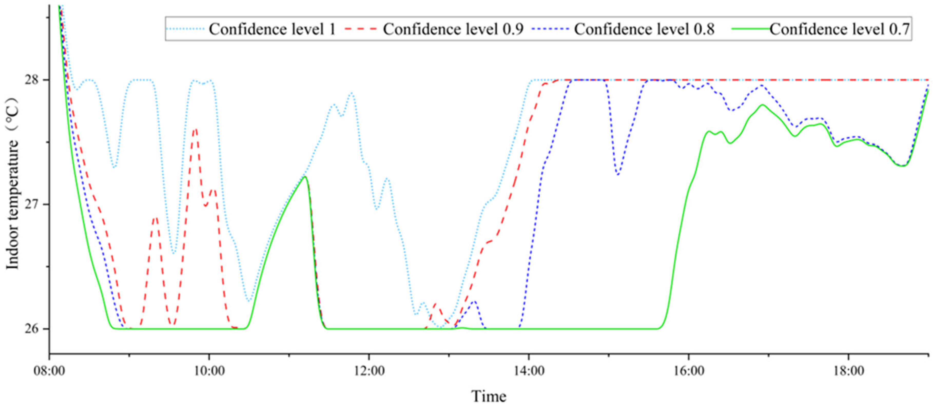
5.3.2. Analysis of the Impact of the Confidence Level on the Optimization Results

Figure 7 shows the indoor temperature optimization results for Scenario 4 with a confidence level ranging from 0.7 to 1. Chance-constrained programming discusses the probability that users will satisfy the constraints when making decisions, while the confidence level reflects the system’s inclination when considering scheduling decisions. A lower confidence level indicates that the system is willing to take on more risk when making decisions, which means that the optimization results will be better. As can be seen from the figure, when the confidence level is 1, the indoor temperature setting is relatively high. This is because, under all possible source-load uncertainties, the decision can satisfy the constraints, which is equivalent to robust optimization. At this point, the decision is conservative, and the indoor thermal comfort is relatively poor. As the confidence level gradually decreases, the generated strategies become more aggressive, and the air-conditioning set temperature gradually decreases. When the confidence level is set to 0.7, the indoor comfort level has already improved significantly compared to when the confidence level is set to 1. However, this decision only has a 70% probability of satisfying the power balance constraint under the source-load uncertainty space, which is relatively aggressive. By reasonably setting the confidence level, it is possible to quantify the decision-maker’s risk preference and balance conservative and aggressive strategies. Overall, a higher confidence level means a lower tolerance for risk that can be assumed, and the overall optimization result will tend to be conservative. Lower confidence means a higher tolerance of risk that can be assumed, and the optimization result will not tend to be conservative. When the confidence level is set to 0.9, extreme conservatism and extreme aggressiveness can be avoided, which corresponds to the occasional short-term prediction deviations in practical engineering, and these deviations can be dynamically corrected by intraday optimization.

6. Conclusions

This paper focuses on the intraday energy optimization of zero-carbon buildings under the fuzzy space of source-load uncertainty, aiming to address the issues of overly conservative day-ahead scheduling plans and the impact of intraday source-load prediction data fuzziness on building energy management. This research represents the source-load fuzziness of zero-carbon buildings using membership functions and employs FCCP to handle uncertain constraints under the fuzzy space. By reasonably setting the confidence level and fuzzy space parameters, decision-makers can choose energy plans with certain risks according to their own needs. The proposed method maximizes indoor thermal comfort through goal programming while balancing the power adjustment of energy storage, thereby mitigating the conservativeness of day-ahead decisions. A more forward-looking intraday energy optimization approach dynamically adjusts the daily scheduling plan based on short-term prediction data. The effectiveness of the method proposed in this paper is verified through case analysis. The results show that compared with the target setting of tracking the day-ahead plan, the intraday energy optimization method that prioritizes thermal comfort increases the average indoor temperature setting from 27.23 °C to 26.32 °C, validating the effectiveness of the proposed method. By comparing the optimization results under different confidence levels and fuzzy parameters, it is demonstrated that FCCP can quantify the decision-maker’s risk preference and balance conservative and aggressive strategies.

References

1. Falana, J.; Osei-Kyei, R.; Tam, V.W. Towards Achieving a Net Zero Carbon Building: A Review of Key Stakeholders and Their Roles in Net Zero Carbon Building Whole Life Cycle. J. Build. Eng. 2024, 82, 108223. [Google Scholar] [CrossRef]
2. Huang, J.; Lu, H.; Du, M. Regional Differences in Agricultural Carbon Emissions in China: Measurement, Decomposition, and Influencing Factors. Land 2025, 14, 682. [Google Scholar] [CrossRef]
3. Al-Ghussain, L.; Abubaker, A.M.; Ahmad, A.D. Superposition of Renewable-Energy Supply from Multiple Sites Maximizes Demand-Matching: Towards 100% Renewable Grids in 2050. Appl. Energy 2021, 284, 116402. [Google Scholar] [CrossRef]
4. Song, Y.; Mu, H.; Li, N.; Wang, H.; Kong, X. Optimal Scheduling of Zero-Carbon Integrated Energy System Considering Long-and Short-Term Energy Storages, Demand Response, and Uncertainty. J. Clean. Prod. 2024, 435, 140393. [Google Scholar] [CrossRef]
5. Wang, L.; Lin, J.; Dong, H.; Wang, Y.; Zeng, M. Demand Response Comprehensive Incentive Mechanism-Based Multi-Time Scale Optimization Scheduling for Park Integrated Energy System. Energy 2023, 270, 126893. [Google Scholar] [CrossRef]
6. Zhu, X.; Hu, M.; Xue, J.; Li, Y.; Han, Z.; Gao, X.; Wang, Y.; Bao, L. Research on Multi-Time Scale Integrated Energy Scheduling Optimization Considering Carbon Constraints. Energy 2024, 302, 131776. [Google Scholar] [CrossRef]
7. Shen, X.; Guo, Q.; Sun, H. Regional Integrated Energy System Planning Considering Energy Price Uncertainties: A Two-Stage Stochastic Programming Approach. Energy Procedia 2019, 158, 6564–6569. [Google Scholar] [CrossRef]
8. Dorahaki, S.; Rashidinejad, M.; Ardestani, S.F.F.; Abdollahi, A.; Salehizadeh, M.R. A Home Energy Management Model Considering Energy Storage and Smart Flexible Appliances: A Modified Time-Driven Prospect Theory Approach. J. Energy Storage 2022, 48, 104049. [Google Scholar] [CrossRef]
9. Onishi, V.C.; Antunes, C.H.; Fraga, E.S.; Cabezas, H. Stochastic Optimization of Trigeneration Systems for Decision-Making under Long-Term Uncertainty in Energy Demands and Prices. Energy 2019, 175, 781–797. [Google Scholar] [CrossRef]
10. Yamamoto, S.; Furukakoi, M.; Uehara, A.; Mikhaylov, A.; Mandal, P.; Senjyu, T. MPC-Based Robust Optimization of Smart Apartment Building Considering Uncertainty for Conservative Reduction. Energy Build. 2024, 318, 114461. [Google Scholar] [CrossRef]
11. Wang, Y.; Song, M.; Jia, M.; Li, B.; Fei, H.; Zhang, Y.; Wang, X. Multi-Objective Distributionally Robust Optimization for Hydrogen-Involved Total Renewable Energy CCHP Planning under Source-Load Uncertainties. Appl. Energy 2023, 342, 121212. [Google Scholar] [CrossRef]
12. Zhen, J.; Liu, X.; Wu, C.; Ji, L.; Huang, G. Operation Optimization and Performance Evaluation of Photovoltaic-Wind-Hydrogen-Based Integrated Energy System under Carbon Trading Mechanism and Uncertainty for Urban Communities. J. Clean. Prod. 2024, 476, 143688. [Google Scholar] [CrossRef]
13. Nikpour, A.; Nateghi, A.; Shafie-khah, M.; Catalão, J.P.S. Day-Ahead Optimal Bidding of Microgrids Considering Uncertainties of Price and Renewable Energy Resources. Energy 2021, 227, 120476. [Google Scholar] [CrossRef]
14. Bakhtiari, H.; Zhong, J.; Alvarez, M. Predicting the Stochastic Behavior of Uncertainty Sources in Planning a Stand-Alone Renewable Energy-Based Microgrid Using Metropolis–Coupled Markov Chain Monte Carlo Simulation. Appl. Energy 2021, 290, 116719. [Google Scholar] [CrossRef]
15. Lin, S.; Liu, C.; Shen, Y.; Li, F.; Li, D.; Fu, Y. Stochastic Planning of Integrated Energy System via Frank-Copula Function and Scenario Reduction. IEEE Trans. Smart Grid 2022, 13, 202–212. [Google Scholar] [CrossRef]
16. Eingartner, A.; Naumann, S.; Schmitz, P.; Worthmann, K. Adjustable Robust Energy Operation Planning under Uncertain Renewable Energy Production. Energies 2024, 17, 1917. [Google Scholar] [CrossRef]
17. Chen, Y.; Chen, C.; Ma, J.; Qiu, W.; Liu, S.; Lin, Z.; Qian, M.; Zhu, L.; Zhao, D. Multi-Objective Optimization Strategy of Multi-Sources Power System Operation Based on Fuzzy Chance Constraint Programming and Improved Analytic Hierarchy Process. Energy Rep. 2021, 7, 268–274. [Google Scholar] [CrossRef]
18. Bi, C.; Chen, J.; Wang, Y.; Feng, L. Fuzzy Credibility Chance-Constrained Multi-Objective Optimization for Multiple Transactions of Electricity–Gas–Carbon under Uncertainty. Electr. Power Syst. Res. 2025, 238, 111089. [Google Scholar] [CrossRef]
19. Jing, Z.; Chen, X.; Bu, L.; Xu, W.; Chen, J.; Yu, K.; Shen, J. Intelligent optimization for building energy management considering indoor heat transfer. Innov. Energy 2024, 1, 100058. [Google Scholar] [CrossRef]
20. Cao, S.; Li, X.; Yang, B. Heat and Moisture Transfer of Building Envelopes under Dynamic and Steady-State Operation Mode of Indoor Air Conditioning. J. Build. Eng. 2021, 44, 102683. [Google Scholar] [CrossRef]
21. Dong, H.; Xu, C.; Chen, W. Modeling and Configuration Optimization of the Rooftop Photovoltaic with Electric-Hydrogen-Thermal Hybrid Storage System for Zero-Energy Buildings: Consider a Cumulative Seasonal Effect. Build. Simul. 2023, 16, 1799–1819. [Google Scholar] [CrossRef]
22. Zong, X.; Zou, S.; Zhou, H.; Dou, X. Robust Stochastic Low-Carbon Optimal Dispatch of Park-Integrated Energy System with Multiple Uncertainties from Source and Load. Front. Energy Res. 2023, 11, 1226768. [Google Scholar] [CrossRef]
23. Liu, H.; Fang, Z.; Li, R. Credibility-Based Chance-Constrained Multimode Resource-Constrained Project Scheduling Problem under Fuzzy Uncertainty. Comput. Ind. Eng. 2022, 171, 108402. [Google Scholar] [CrossRef]
24. Li, P.; Wang, X.; Han, P. Risk Analysis of Microgrid Optimal Operation Scheduling Under Double Uncertainty Environment. Proc. CSEE 2017, 37, 4296–4303. [Google Scholar] [CrossRef]
Figure 1. Intraday energy optimization of zero-carbon buildings.
Energies 18 02582 g001
Figure 2. Zero-carbon building intraday energy optimization flow chart.
Energies 18 02582 g002
Figure 3. Zero-carbon building source-load power and outdoor temperature curve.
Energies 18 02582 g003
Figure 4. BESS charge and discharge power curve.
Energies 18 02582 g004
Figure 5. Indoor temperature setting curves under different examples.
Energies 18 02582 g005
Figure 6. Indoor temperature setting curves under different degrees of ambiguity.
Energies 18 02582 g006
Figure 7. Indoor temperature setting curves at different confidence levels.
Energies 18 02582 g007