Pathways to Positive Energy Districts: A Comprehensive Techno-Economic and Environmental Analysis Using Multi-Objective Optimization

Abstract

Transitioning to Positive Energy Districts (PEDs) is essential for achieving carbon neutrality in urban areas by 2050. This study presents a multi-objective optimization framework that balances energy, environmental, and economic performance, addressing the diverse priorities of multiple stakeholders. The framework enhances PED design by systematically evaluating technical solutions, including renewable-based electrification, demand-side management (DSM), energy storage, and retrofitting. The framework is applied to the Usquare district in Brussels, Belgium, as a case study. The results indicate that expanding photovoltaic (PV) capacity is crucial for achieving PED targets, with renewable-based electrification potentially reducing carbon emissions by up to 79%. The incorporation of demand-side management (DSM) and battery storage improves system flexibility, reduces grid dependency, and enhances cost-effectiveness. Although slightly more costly, retrofitting existing buildings provides the most balanced approach, offering the lowest CO2 emissions and the highest self-consumption ratio. This study presents a comprehensive decision-making support framework for optimizing PED design and operation, offering practical guidance for urban energy planning and contributing to global efforts toward carbon neutrality.

1. Introduction

The reduction in greenhouse gas (GHG) emissions is a global need that addresses the challenges of the energy transition. The International Energy Agency (IEA) reports that, as of 2021, urban areas contributed to nearly 75% of worldwide primary energy use and accounted for around 70% of total GHG emissions [1]. In the context of the European Union (EU), cities are projected to account for approximately 90% of the increase in global energy demand in the coming years [2]. Given their significant impact, cities are crucial in achieving ambitious net-zero emissions targets. In this context, research on Positive Energy Districts (PEDs) has gained momentum in recent years. The PED concept was introduced in the European Strategic Energy Technology (SET) Plan in 2018 [3], with the goal of establishing 100 Positive Energy Districts across Europe by 2025. The PED initiative is supported by various programs, including the Joint Programming Initiative (JPI) Urban Europe [4], and the IEA Energy in Buildings and Communities (EBC) Annex 83, extending its reach beyond Europe [5].

1.1. Concept of Positive Energy Districts

The concept of Positive Energy Districts (PEDs) was first introduced under Action 3.2 of the SET-Plan, titled “Smart Cities and Communities” [6]. These districts are designed to achieve net-zero energy imports and carbon emissions on an annual basis. The primary objectives of PEDs are closely linked to achieving energy balance and carbon neutrality [7], and they are categorized into different typologies: autonomous, dynamic, and virtual PED boundaries [8].

The reference framework for PEDs/PENs [4] extends this definition by establishing PEDs/PENs as a framework structured around three most important functions: energy production, energy efficiency, and energy flexibility. Rather than concentrating merely on balancing energy supply and demand [9], this framework underscores the importance of integrating diverse systems and infrastructures. It also highlights the need for active interaction among buildings, users, and regional energy, mobility, and ICT systems. This integration aims to ensure energy security and enhance quality of life while aligning with goals for social, economic, and environmental sustainability [4].

1.2. Metrics and Benchmarks for Assessing PEDs

The foundation of PED concepts is the energy balance [10], defined as the difference between energy consumption and production within specific geographical or virtual boundaries [9]. A key aspect of PED assessments is the quantifiable metric used to compare energy flows among different energy carriers within a district [7]. To accurately calculate the energy balance, all energy components must be converted using a consistent metric. Various metrics have been explored in the literature, with primary energy [11,12] and $\mathrm{C}{\mathrm{O}}_2$ equivalent emissions [5,13] being the most commonly employed. These metrics are particularly important when comparing PED outcomes across different regions, as they are directly influenced by carbon emission factors and the specific characteristics of national energy production systems [9,14].

1.3. Engaging Multiple Stakeholders of PEDs

In the broader context of Sustainable Development Goals (SDGs), the concept of PEDs has evolved into a more complex framework that emphasizes a shift from single environmental goals to comprehensive analyses, along with increased stakeholder involvement in the design process [9]. Therefore, establishing a common vision and shared objectives among stakeholders is crucial to driving the energy transition process [15]. For example, the syn.ikia project [16,17] proposes a framework that defines five key performance indicator (KPI) categories for evaluating Sustainable Plus Energy Neighborhoods, including energy and environmental performance, economic performance, indoor environmental quality, social aspects, and smartness and flexibility. Similarly, Volpe et al. [18] emphasize the importance of KPIs in achieving SDGs, defining them based on three main dimensions: membership, sustainability assessment, and technology and operation. Sassenou et al. [7] provide a framework known as PlanPED for planning, designing, and implementing PEDs, including stakeholder management, to support municipalities in their energy transition. The PlanPED framework [7] identifies four primary KPI categories for evaluating PED projects: energy performance (EnerP), environmental performance (EnviP), economic performance (EcoP), and social performance and quality of life.

1.4. Integration of Technical Solutions

By definition, in [4], PEDs should integrate diverse solutions, requiring the coordination of energy resources and assets to optimize efficiency, renewable generation, flexibility, and cost-effectiveness [5]. IEA EBC Annex83 [19] reviewed the concept of positive energy globally, including Zero-Energy Buildings and Nearly Zero Energy Districts. The review delved into energy flexibility, highlighting aspects such as hybrid energy storage, intelligent controls, demand-side management, and connection to the energy grid. Heller [20] showcased the most common technical solutions for urban districts, ordered by their function from high technology readiness levels (TRLs) to low TRLs.

First, photovoltaic (PV) systems are among the most widespread technologies adopted in the energy transition, with numerous studies investigating the integration of PV systems in PEDs. According to the onion model developed by Lindholm et al. [8], achieving dynamic PEDs in urban cores with high energy density and limited renewable energy sources (RESs) is challenging. Instead, virtual boundaries are implemented in PEDs, allowing them to own and operate renewable energy systems and storage outside their geographical boundaries. Guarino et al. [6] explored the feasibility of renovating existing buildings into PEDs in Balaguer, Spain. The results highlighted that renovations significantly improved performance, leading to substantial reductions in overall primary energy consumption. However, they noted that achieving PEDs for low-story buildings would require at least double the available solar PV area, even with renovations.

Furthermore, research highlights the critical importance of retrofitting buildings to improve energy performance, particularly given that 75% of the EU building stock is classified as inefficient [12]. Gouveia et al. [21] explored the potential of renovation measures and building-integrated photovoltaics (BIPV) in historic districts in Lisbon, Portugal, showing that retrofitting can reduce space heating and cooling demand by up to 84% and 19% annually, respectively.

Additionally, demand-side management and energy storage are key strategies for enhancing the resilience and flexibility of regional energy systems. Guasselli et al. [22] highlight the critical role of smart technologies and demand-side management in PED/Positive Energy Neighborhood (PEN) projects, demonstrated through a case study in Norway. Similarly, Maratta et al. [23] investigate the potential of energy retrofitting, renewable energy integration, and energy flexibility activation to achieve PED in Southern Italy. Their study shows that activating energy flexibility can reduce operational $C{O}_2,eq$ emissions by 10% while increasing energy self-consumption.

1.5. Tools and Methods for PED Optimal Design

The design of PEDs is a complex and dynamic process that requires diverse solutions to address the needs of different target users during the early-stage planning [7]. Optimization-based design methods are particularly valuable as they provide efficient tools for identifying the best system configurations over a large time horizon, enabling cost-effective exploration of PED potential. Bruck et al. [24] proposed a mixed-integer linear program (MILP) to optimally design and operate PEDs with maximum net present value (NPV), comparing electrified PED solutions across different EU zones. Based on this work, Bruck et al. [12] extended the model to analyze the impact of retrofitting PED projects across several case studies from a techno-economic perspective. Volpe et al. [13] proposed an optimization model to evaluate optimal energy distribution flows within the districts for PEDs. Laitinen et al. [25] developed an optimization method to balance life-cycle costs and self-sufficiency (SSR) in a Helsinki district, concluding that positive energy zones are more practical than full energy self-sufficiency economically and technically.

1.6. Scope of This Work

The state-of-the-art review highlights several published studies focusing on PEDs and related concepts [5]. Table 1 provides a summary of relevant studies in the literature, detailing key performance indicators (KPIs), evaluation metrics, combination of solutions, and methodologies employed in PED design. However, despite these contributions, as shown in Table 1, significant gaps remain in the development of a comprehensive optimization framework for PED design, including: (1) Limited integration of techno-economic and environmental objective optimization for the early-stage planning of PEDs. (2) A lack of comparative analysis on stand-alone and combined technical solutions (e.g., renewable-based electrification, demand-side management, energy storage) in achieving PED targets.

Table 1. Literature review of recent studies on the Positive Energy Districts and related concepts.

Reference	KPIs 1			Evaluation	Solutions 3					Method 4	Location
	EnerP	EnviP	EcoP	Metric 2	RES	Sto	Retro	DSM	Elect
Marrasso et al. [26]	Y	Y		$\mathrm{C}{\mathrm{O}}_2$	STC,	TES,				-	Italy
					PV, WT	PtH2
Bruck et al. [2]	Y	Y	Y	PEF	PV	BAT				MILP	Spain
Bruck et al. [12]	Y	Y	Y	PEF	PV		Y		Y	MILP	Spain
											Germany
											Sweden
Laitinen et al. [25]	Y	Y	Y	$\mathrm{C}{\mathrm{O}}_2$	PV, WT	BAT			Y	LP	Finland
Blumberga et al. [27]	Y	Y		PEF	PV	BAT				-	Latvia
An et al. [28]	Y	Y		$\mathrm{C}{\mathrm{O}}_2$	BIPV		Y		Y	-	South Korea
Guarino et al. [6]	Y	Y		$\mathrm{C}{\mathrm{O}}_2$	PV		Y			-	Spain
Gouveia et al. [21]	Y	Y	Y	$\mathrm{C}{\mathrm{O}}_2$	BIPV		Y			-	Portugal
Bambara et al. [29]	Y	Y		PEF	BIPV		Y		Y	-	Canada
Volpe et al. [13]	Y	Y		$\mathrm{C}{\mathrm{O}}_2$	PV, BIO		Y			-	Italy
Guasselli et al. [22]	Y	Y		$\mathrm{C}{\mathrm{O}}_2$	PV, GEO			Y	Y	-	Norway

¹ EnerP: energy performance, EnvirP: environmental performance, EcoP: economic performance. ² PEF: Primary Energy Factor. ³ RES: renewable energy source, Sto: storage, Retro: retrofit, DSM: demand-side management, Elect: electrification, STC: evacuated tube collectors, PV: photovoltaic, BIPV: building-integrated photovoltaics, WT: wind turbine, BIO: biomass, GEO: geothermal, BAT: battery, PtH2: power-to-hydrogen. ⁴ MILP: Mixed-Integer Linear Programming, LP: Linear Programming.

Table 1. Literature review of recent studies on the Positive Energy Districts and related concepts.

Reference	KPIs 1			Evaluation	Solutions 3					Method 4	Location
	EnerP	EnviP	EcoP	Metric 2	RES	Sto	Retro	DSM	Elect
Marrasso et al. [26]	Y	Y		$\mathrm{C}{\mathrm{O}}_2$	STC,	TES,				-	Italy
					PV, WT	PtH2
Bruck et al. [2]	Y	Y	Y	PEF	PV	BAT				MILP	Spain
Bruck et al. [12]	Y	Y	Y	PEF	PV		Y		Y	MILP	Spain
											Germany
											Sweden
Laitinen et al. [25]	Y	Y	Y	$\mathrm{C}{\mathrm{O}}_2$	PV, WT	BAT			Y	LP	Finland
Blumberga et al. [27]	Y	Y		PEF	PV	BAT				-	Latvia
An et al. [28]	Y	Y		$\mathrm{C}{\mathrm{O}}_2$	BIPV		Y		Y	-	South Korea
Guarino et al. [6]	Y	Y		$\mathrm{C}{\mathrm{O}}_2$	PV		Y			-	Spain
Gouveia et al. [21]	Y	Y	Y	$\mathrm{C}{\mathrm{O}}_2$	BIPV		Y			-	Portugal
Bambara et al. [29]	Y	Y		PEF	BIPV		Y		Y	-	Canada
Volpe et al. [13]	Y	Y		$\mathrm{C}{\mathrm{O}}_2$	PV, BIO		Y			-	Italy
Guasselli et al. [22]	Y	Y		$\mathrm{C}{\mathrm{O}}_2$	PV, GEO			Y	Y	-	Norway

¹ EnerP: energy performance, EnvirP: environmental performance, EcoP: economic performance. ² PEF: Primary Energy Factor. ³ RES: renewable energy source, Sto: storage, Retro: retrofit, DSM: demand-side management, Elect: electrification, STC: evacuated tube collectors, PV: photovoltaic, BIPV: building-integrated photovoltaics, WT: wind turbine, BIO: biomass, GEO: geothermal, BAT: battery, PtH2: power-to-hydrogen. ⁴ MILP: Mixed-Integer Linear Programming, LP: Linear Programming.

To address this gap, this paper extends our previous work [30] by introducing a multi-objective optimization framework that integrates energy, environmental, and economic KPIs. This paper aims to answer the following research questions:

• Which metrics and benchmarks are used to assess PEDs?
• For a specific case, what are the feasible solutions to achieve PEDs?
• What is the most cost-effective pathway to implementing PEDs in specific scenarios?

To answer these questions, the research objective of this study is to introduce a novel approach for the techno-economic and environmental analysis of various scenarios through an optimization framework designed for the early-stage planning and pre-designing of PEDs. Focusing on a specific case study, this study aims to enhance the understanding of how multiple solutions can be integrated into renewable-based energy systems and explore pathways to achieving PEDs. It also seeks to provide a decision-support tool that helps stakeholders identify the most viable solutions based on their diverse priorities.

The paper is organized as follows: the optimization framework is presented in Section 2, followed by the results of a case study in Section 3, and a discussion in Section 4. The conclusions are provided in Section 5.

2. Methodology

First, the overview of the system framework, originally presented in our previous work [30], is described. Following that, the assumptions and scenarios for the selected case study are outlined.

2.1. System Framework

Figure 1 illustrates the modeling framework for the pre-design of PEDs. This framework consists of the following components: First, data collection, gathering input data using appropriate tools (Figure 1a). Second, boundary identification and scenario generation, defining PED boundaries and generating scenarios based on the configuration of selected solutions. Next, optimization execution, implementing the optimization framework separately using multi-objective optimization and PED constraints. Finally, discussion of the results, analyzing and discussing the results.

Figure 1. Optimization framework for Positive Energy District projects. Abbreviations: Positive Energy District (PED), Primary Energy Factor (PEF).

The general layout of the hybrid renewable energy system (HRES) is shown in Figure 2. In the current system, the electricity demand is only provided by the grid, and heating demand is served by a natural gas boiler operating at 70 °C. The cooling demand is met by an electrical chiller. In the optimal energy system to be designed, PV panels (for power), a natural-gas fired CHP (for power and high-temperature heat), as well as air-sourced heat pumps and geothermal heat pumps (for low-temperature heat) are considered as available options. The HRES is connected to the electricity grid, enabling both energy import and export. All buildings are linked to a decentralized heating network. Further details are provided in Section 2.5.

Figure 2. Schematic diagram of the considered hybrid renewable energy system.

2.2. Mathematical Model

The optimization problem was formulated as a Mixed-Integer Linear Programming (MILP) model, which determined the optimal selection, sizing, and operation of the considered technologies. The epsilon-constraint method was used to explore trade-offs between economic and environmental objectives, ensuring that the energy system design was cost-effective and sustainable. The MILP formulation included constraints and variables representing each technology’s technical and operational characteristics, as well as their interactions within the system. A detailed description of the optimization problem is provided in Appendix A.

$$\begin{array}{cc}\hfill & \min f_1(x({ϵ}_j))\hfill \\ \hfill & \mathrm{subject}\mathrm{to}:\hfill \\ \hfill & g\left(x\right)\le 0\hfill \\ \hfill & f_2(x({ϵ}_j))\le {ϵ}_j\hfill \\ \hfill & f_2{\left(x\right)}^{\min }\le {ϵ}_j\le f_2{\left(x\right)}^{\max }\forall {ϵ}_j\in \{{ϵ}_1,{ϵ}_2,\cdots ,{ϵ}_n\}\hfill \end{array}$$

(1)

where x is the vector of decision variables. $f_1(x)$ represents the first objective (e.g., TAC), and $f_2(x)$ represents the constrained objective functions. ${ϵ}_j$ is a predefined threshold that restricts $f_2\left(x\right)$. The upper ($f_2{\left(x\right)}^{\max }$) and lower ($f_2{\left(x\right)}^{\min }$) limits of ${ϵ}_j$ can be determined by solving two single-objective optimizations separately.

2.3. Objective Functions

This study aimed to optimize the sizing and operation of the HRES to minimize total annual cost (TAC) and carbon emissions (CE). The calculations for TAC and CE are detailed in the following sections.

2.3.1. Total Annual Cost

The TAC is calculated as the total costs of the energy system, excluding the revenue. It includes capital expenditures (CAPEXs), operational expenditures (OPEX), $\mathrm{C}{\mathrm{O}}_2$ tax (${\mathrm{C}}_{\mathrm{C}{\mathrm{O}}_2,a}$), gas costs ($C_{\mathrm{gas},a}$), electricity costs ($C_{\mathrm{el},a}$), and revenue from electricity feed-in ($R_{\mathrm{el},a}$). Mathematically, the TAC can be expressed as:

$$\mathrm{TAC}=C_{\mathrm{CAPEX},a}+C_{\mathrm{OPEX},a}+C_{\mathrm{el},a}+C_{\mathrm{gas},a}+C_{\mathrm{C}{\mathrm{O}}_2,a}-R_{\mathrm{el},a}$$

(2)

The annualized investment cost, ${\mathrm{CAPEX}}_a$, is described by:

$${\mathrm{CAPEX}}_a=\mathrm{CRF}·\sum _{k\in \mathrm{K}}{\mathrm{Cap}}_k·{\mathrm{CAPEX}}_k$$

(3)

where k refer to the different components, and $\mathrm{Cap}$ refers to the installed capacity of each component. The capital recovery factor (CRF) is determined by the interest rate i and the system lifetime L and is expressed as:

$$\mathrm{CRF}={\displaystyle \frac{i·{(1+i)}^L}{{(1+i)}^L-1}}$$

(4)

In addition to the annualized investment cost, the annualized operating cost, ${\mathrm{OPEX}}_a$, is expressed as a proportion $d_k$ of the annualized investment cost:

$${\mathrm{OPEX}}_a=\sum _{k\in \mathrm{K}}{d}_k·{\mathrm{CAPEX}}_k$$

(5)

The fuel cost is calculated by:

$$C_{\mathrm{gas},a}=\sum _{d\in \mathrm{D}}{w}_d\sum _{t\in \mathrm{T}}\left(G_{\mathrm{BOI},d,t}+G_{\mathrm{CHP},d,t}\right)·p_{\mathrm{gas}}·\mathrm{\Delta }t$$

(6)

where $\mathrm{\Delta }t$ is the duration of the time step, $w_d$ are the weighting factors for each design day, referring to the number of days in a year that a specific design day represents, $p_{\mathrm{gas}}$ is the natural gas supply price (EUR/kWh), and G is the amount of gas purchased for a single time step.

Similarly, the electricity supply cost $C_{\mathrm{el},a}$ is determined by the supply price ($p_{\mathrm{elec}}$) and electricity purchased from the grid ($P_{\mathrm{grid},d,t}$):

$$C_{\mathrm{el},a}=\sum _{d\in \mathrm{D}}{w}_d\sum _{t\in \mathrm{T}}{P}_{\mathrm{grid},d,t}·p_{\mathrm{elec}}·\mathrm{\Delta }t$$

(7)

The feed-in revenue $R_{\mathrm{el},a}$ is calculated based on the feed-in tariff ($p_{\mathrm{feed}\text{-}\mathrm{in}}$) and electricity sold to the grid ($P_{\mathrm{feed}\text{-}\mathrm{in},d,t}$):

$$R_{\mathrm{el},a}=\sum _{d\in \mathrm{D}}{w}_d\sum _{t\in \mathrm{T}}{P}_{\mathrm{feed}\text{-}\mathrm{in},d,t}·p_{\mathrm{feed}\text{-}\mathrm{in}}·\mathrm{\Delta }t$$

(8)

The $C{O}_2$ cost is determined by the $\mathrm{C}{\mathrm{O}}_2$ emissions and CO2 tax:

$$C_{\mathrm{C}{\mathrm{O}}_2,a}=\left({\mathrm{C}{\mathrm{O}}_2}_{\mathrm{grid},a}+{\mathrm{C}{\mathrm{O}}_2}_{\mathrm{NG},a}\right)·p_{{\mathrm{C}{\mathrm{O}}_2}_{tax}}$$

(9)

2.3.2. Carbon Emissions

The carbon emissions (CE) are calculated as the annualized total $\mathrm{C}{\mathrm{O}}_2$ emissions of the energy system. The annual carbon emissions consist of two components: $\mathrm{C}{\mathrm{O}}_2$ emissions result from grid connection (${\mathrm{CO}}_{2,\mathrm{grid},\mathrm{a}}$) and $\mathrm{C}{\mathrm{O}}_2$ emissions result from gas purchased (${\mathrm{CO}}_{2,\mathrm{NG},\mathrm{a}}$). Mathematically, the carbon emissions can be expressed as:

$$\mathrm{CE}={\mathrm{C}{\mathrm{O}}_2}_{\mathrm{grid},a}+{\mathrm{C}{\mathrm{O}}_2}_{\mathrm{NG},a}$$

(10)

2.4. Key Performance Indicators

This section introduces key performance indicators (KPIs) to evaluate the performance of Positive Energy Districts (PEDs), focusing on energy, environmental, and economic assessments.

2.4.1. Evaluation of Financial Profitability

The financial evaluation of energy system projects is crucial for determining their economic viability and ensuring that investments yield satisfactory returns. This process involves assessing various financial metrics, such as net present value (NPV) and internal rate of return (IRR) [31,32].

The NPV, an economic metric of project profitability, is defined as the sum of all cash flows (CF), minus initial investment costs ($I_0$), replacement costs ($I_{\mathrm{rep}}$), and including salvage value ($I_{\mathrm{salvage}}$) over the project lifetime (L) [33,34]. The NPV is expressed as:

$$\mathrm{NPV}=\sum _{n=1}^L{\displaystyle \frac{{\mathrm{CF}}_n}{{(1+i)}^n}}-I_0-I_{\mathrm{rep}}+I_{\mathrm{salvage}}$$

(11)

The cash flow is determined by the difference between cash inflow and cash outflow. Cash inflow ($I_n$) represents the incomes generated, which are related to fuel savings (${\mathrm{C}}_{\mathrm{fuel},a}^{\mathrm{saved}}$), grid savings (${\mathrm{C}}_{\mathrm{grid},a}^{\mathrm{saved}}$), and revenue generation ($R_{\mathrm{el},a}$) compared to the status quo. Cash outflow ($C_n$) represents the total expenses.

$$\begin{array}{cc}\hfill {\mathrm{CF}}_n& =I_n-C_n\hfill \end{array}$$

(12)

$$\begin{array}{cc}\hfill I_n& =C_{\mathrm{fuel},a}^{\mathrm{saved}}+C_{\mathrm{grid},a}^{\mathrm{saved}}+R_{\mathrm{el},a}\hfill \end{array}$$

(13)

$$\begin{array}{cc}\hfill C_n& =C_{\mathrm{OPEX},a}+C_{\mathrm{el},a}+C_{\mathrm{gas},a}+C_{\mathrm{C}{\mathrm{O}}_2,a}\hfill \end{array}$$

(14)

The replacement cost represents the cost of replacing components during the system lifetime and is expressed as [35]:

$$I_{\mathrm{rep}}=\sum _{k=0}^K\left(C_{\mathrm{replace},k}·\sum _{l=1}^{r_k}{\displaystyle \frac{1}{{(1+i)}^{l·t_k}}}\right)$$

(15)

where $C_{\mathrm{replace},k}$ is the cost of component k during each replacement. $r_k$ is the number of replacements during the system lifetime for every component, and $t_k$ is the replacement period(lifetime) for component k.

The salvage value (SV), also known as residual value, represents the remaining value of components that have not reached the end of their lifetime [36]. Salvage values can mitigate end-of-horizon effects [37]. The equation for salvage value is [34]:

$$I_{\mathrm{salvage}}=\sum _{k=0}^{\mathrm{K}}{\displaystyle \frac{C_{\mathrm{salvage},k}}{{(1+i)}^L}}$$

(16)

where $C_{\mathrm{salvage},k}$ is the residual value of component k at the end of the project lifetime.

The internal rate of return (IRR) is a financial metric used to estimate the profitability of potential investments. The IRR is the discount rate that makes the NPV of the project equal to zero. Generally, when comparing investment options with similar characteristics, the higher the IRR, the more desirable the investment. The equation for the IRR is:

$$0=\sum _{n=1}^L{\displaystyle \frac{C{F}_n}{{(1+\mathrm{IRR})}^n}}-I_0-I_{\mathrm{rep}}+I_{\mathrm{salvage}}$$

(17)

2.4.2. Evaluation of PEDs’ Carbon Neutrality

To evaluate the carbon neutrality of an energy system, the Carbon Neutrality Check (CNC) index is used [26]. This indicator compares the $\mathrm{C}{\mathrm{O}}_2$ emissions due to energy supply in the district (${\mathrm{C}{\mathrm{O}}_2}^{\mathrm{in}}$) to the emissions credit from surplus energy supplied by RES-based units (${\mathrm{C}{\mathrm{O}}_2}^{\mathrm{Cred}}$). The difference between the $\mathrm{C}{\mathrm{O}}_2$ emissions and $\mathrm{C}{\mathrm{O}}_2$ credits is normalized against the maximum value between ${\mathrm{C}{\mathrm{O}}_2}^{\mathrm{in}}$ and ${\mathrm{C}{\mathrm{O}}_2}^{\mathrm{Cred}}$. A negative CNC indicates an emission credit, meaning the district can be considered a PED. The closer the CNC is to −1, the higher the share of renewable energy generated. Conversely, a positive CNC means that carbon neutrality has not been achieved, with a CNC closer to 1 indicating less penetration of renewable energy.

$$\mathrm{CNC}={\displaystyle \frac{{\mathrm{C}{\mathrm{O}}_2}^{\mathrm{in}}-{\mathrm{C}{\mathrm{O}}_2}^{\mathrm{Cred}}}{max({\mathrm{C}{\mathrm{O}}_2}^{\mathrm{in}},{\mathrm{C}{\mathrm{O}}_2}^{\mathrm{Cred}})}}$$

(18)

2.4.3. Self-Sufficient Ratio

The Self-Sufficiency Ratio (SSR) is a critical indicator that measures the extent to which a renewable energy system can meet the total energy demands of a district. Specifically, the SSR represents the fraction of the total load—comprising electricity, heating, and cooling demands—that is supplied by the renewable energy system rather than relying on external sources like the grid [38,39]. A higher SSR indicates a greater degree of energy independence within the system.

$$\mathrm{SSR}=1-{\displaystyle \frac{{\sum }_{t=0}^N{P}_{\mathrm{grid},t}}{{\sum }_{t=0}^N{P}_{\mathrm{load},t}}}$$

(19)

where $P_{\mathrm{grid},t}$ represents the power drawn from the grid at time t, and $P_{\mathrm{load},t}$ represents the total energy demand at time t. The sum of electricity, heating, and cooling demands characterizes the total annual load.

2.4.4. Self-Consumption Ratio

The self-consumption ratio (SCR) is another critical performance metric that quantifies the proportion of the total energy produced by a PV system that is consumed within the district. It serves as an indicator of how effectively the generated energy is utilized locally [40]. An SCR close to 1 implies that most of the energy produced is consumed on-site, whereas a lower SCR may suggest that the PV system is oversized, or that there is a significant export of surplus energy [41].

$$\mathrm{SCR}={\displaystyle \frac{{\sum }_{t=0}^N{P}_{\mathrm{PV},\mathrm{load},t}}{{\sum }_{t=0}^N{P}_{\mathrm{PV},\mathrm{tot},t}}}$$

(20)

2.4.5. LCOEx

The Levelized Cost of Exergy (LCOEx) is an economic indicator that reflects the cost per unit of exergy supplied by the energy system. Unlike energy, exergy accounts for the quality and usability of energy, making the LCOEx a more precise metric for evaluating the economic efficiency of integrated energy systems [30,42].

$$\mathrm{LCOEx}={\displaystyle \frac{{\mathrm{CAPEX}}_a+{\mathrm{OPEX}}_a+C_{\mathrm{el},a}+C_{\mathrm{C}{\mathrm{O}}_2,a}+C_{\mathrm{fuel},a}}{\mathrm{Ex}}}$$

(21)

The annual exergy provided by the system is the sum of the exergetic content of the delivered energy fluxes (i.e., electricity (elec), cooling (cool), domestic hot water (DHW), and space heating (SH)) [43]:

$$\mathrm{Ex}=\sum _{\mathrm{type}}{X}^{\mathrm{type}}\forall \mathrm{type}\in \{\mathrm{elec},\mathrm{DHW},\mathrm{SH},\mathrm{cool}\}$$

(22)

While electricity is pure exergy, the exergy flux associated with heat and cold production is calculated by multiplying the energy flux by the Carnot factor F [44]:

$$X^{\mathrm{type}}=F^{\mathrm{type}}·E^{\mathrm{type}}\forall \mathrm{type}\in \{\mathrm{DHW},\mathrm{SH},\mathrm{cool}\},$$

(23)

$$F=1-{\displaystyle \frac{T_{\mathrm{C}}}{T_{\mathrm{H}}}},$$

(24)

where $T_{\mathrm{C}}$ denotes the temperature of the cold source, and $T_{\mathrm{H}}$ refers to the hot-source temperature. For heat load, $T_{\mathrm{C}}$ is set as 25 °C, and $T_{\mathrm{H}}$ is the supply temperature for DHW and space heating, set as 40 °C and 35 °C, respectively [42]. Conversely, for cold load, $T_{\mathrm{H}}$ refers to the ambient temperature, and $T_{\mathrm{C}}$ is the cooling supply temperature set as 7°C [43].

2.5. Case Study

The case study focused on the Usquare district in Brussels, Belgium. Usquare is one of the living labs under the Citizens4PED project [45], which aims to transform former barracks into a vibrant and diverse living space in the Brussels-Capital Region [46]. This study centered on 20 buildings within this mixed-use district, covering a total floor area of 54,679 ${\mathrm{m}}^2$, with a maximum available roof area of 10,017 ${\mathrm{m}}^2$ for the installation of PV panels. The district features two distinct thermal energy demands with specific supply and return temperature levels: high-temperature heat (70/50 °C) for domestic hot water and space heating in low-energy performance buildings and low-temperature heat (50/40 °C) used for space heating in high-energy-performance buildings. Hourly data on ambient temperature and solar irradiance were sourced from the Photovoltaic Geographic Information System (PVGIS) [47], the hourly energy demands of these buildings were simulated using nPro [48], which employs standard load profiles based on building typologies, and the corresponding annual energy demands are summarized in Table 2. The sets of input data used in this work, namely, the hourly profile of the solar radiation, the ambient temperature, the energy demand, and the electricity price, are reported in Appendix Figure A1.

Table 2. Energy demand overview of the energy district for one year.

Parameter	Peak Load	Annual Demand
	kW	MWh
Electricity	1188	4201
Space heating (70/50 °C)	2097	2739
Space heating (50/40 °C)	406	569
DHW	328	1170
Cooling	266	379

Additionally, following the methodology of Bruck et al. [24], a grid connection capacity limit of twice the initial maximum power consumption was imposed.

2.6. Investigated Scenarios

This study explored various configurations of solutions by modeling seven different scenarios. All the selected scenarios are summarized in Figure 3 and described in the following:

Figure 3. The scenarios considered in this study. In the optimal energy system to be designed (BASE scenario), high-temperature heat demands are met by a CHP and a BOI. In the Elect scenario, air-source heat pump and geothermal heat pumps (HPs) are considered for high-temperature heat demands.

• BAU. This scenario represented the status quo, with no PV installations. A natural gas boiler supplied high-temperature heat demand, the grid met all electricity demand, and a compression chiller covered cooling demand.
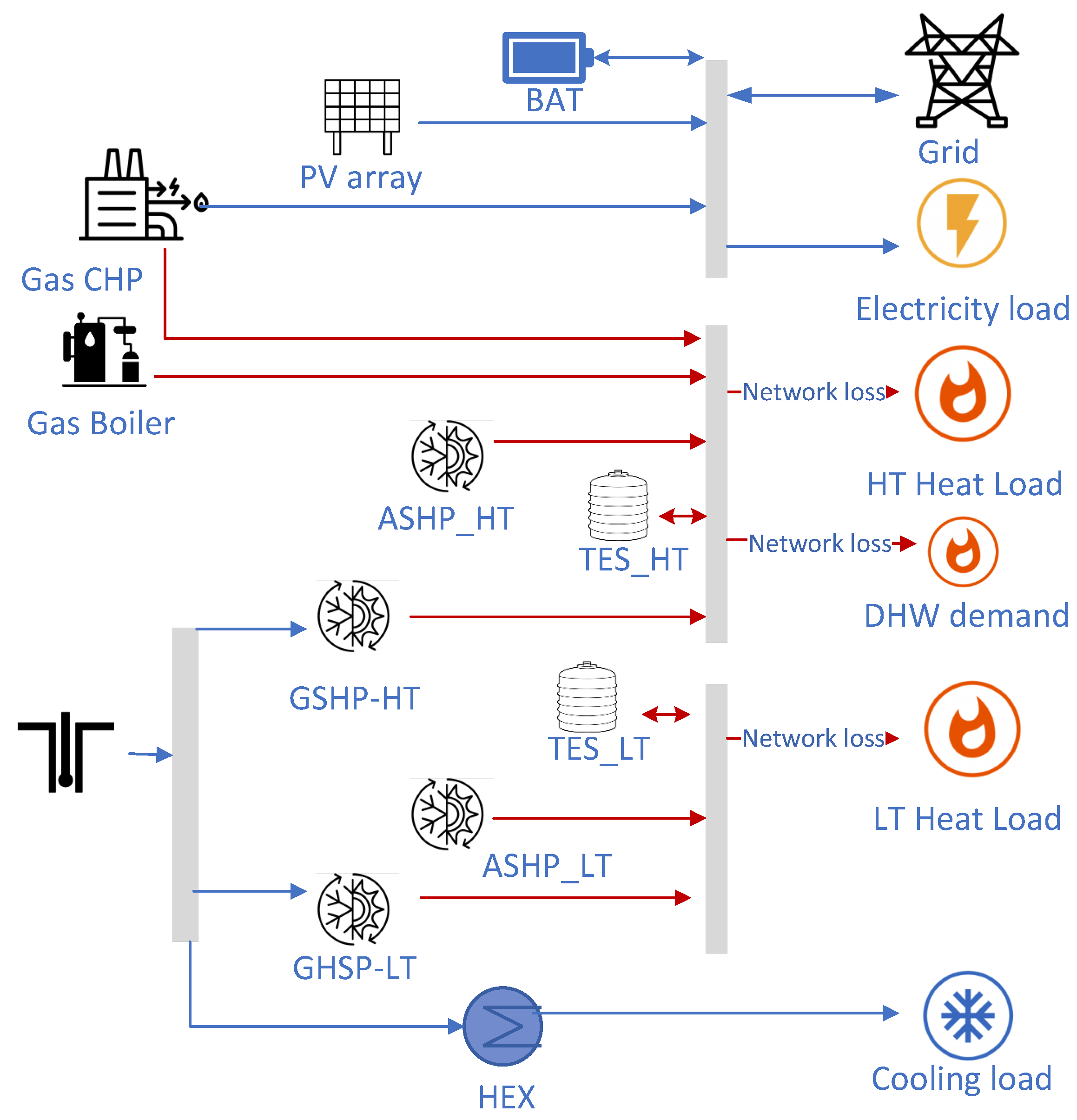
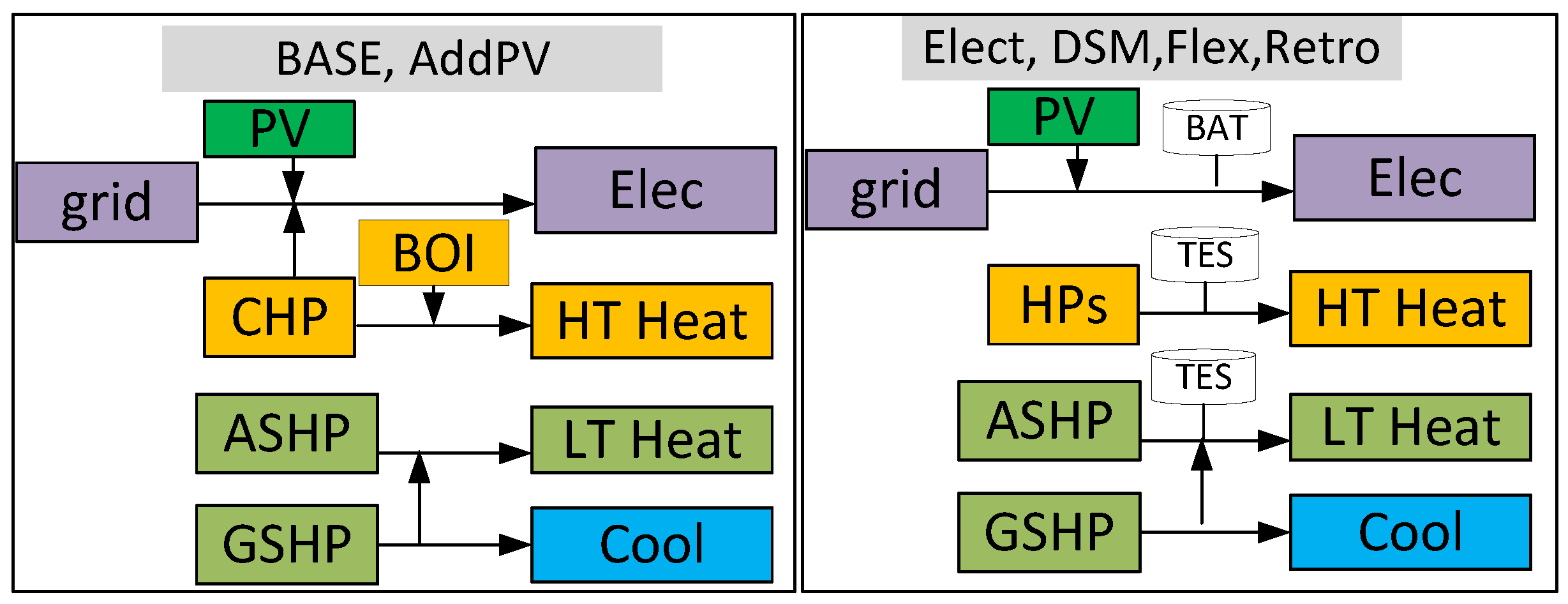
• BASE. The baseline scenario reflected the optimal energy system to be designed, as described in Figure 3. A combination of PV, grid, and a natural-gas CHP met electricity demand. Cooling demand was handled by passive cooling, high-temperature heat demand by a CHP, BOI, and GSHP, and low-temperature heat demand by an ASHP and a GSHP.
• AddPV. In this study, the BASE scenario, limited by available PV roof area, failed to meet carbon-neutral targets. The AddPV scenario addressed this by introducing virtual PEDs, allowing renewable energy imports beyond the geographical boundary. Based on preliminary results, the upper limit of the design variable—the PV roof area—was set at five times the initial capacity to ensure carbon neutrality, although utilizing the maximum area may not be necessary.
• Elect. Additionally to AddPV, this scenario assumed that all energy demands were met by electrical devices, with no NG-based units allowed. Instead, high-temperature heat pumps, including a geothermal heat pump and an air-source heat pump, were utilized to fulfill high-temperature heat demands. This approach is illustrated in Figure 3.
• DSM. In addition to Elect, this scenario incorporated demand response by shifting electricity demand with a dynamic time-of-use (TOU) tariff. A detailed description of the approach is described in Appendix A.4.2.
• Flex. Building on DSM, this scenario included battery storage to utilize energy surplus [10] properly.
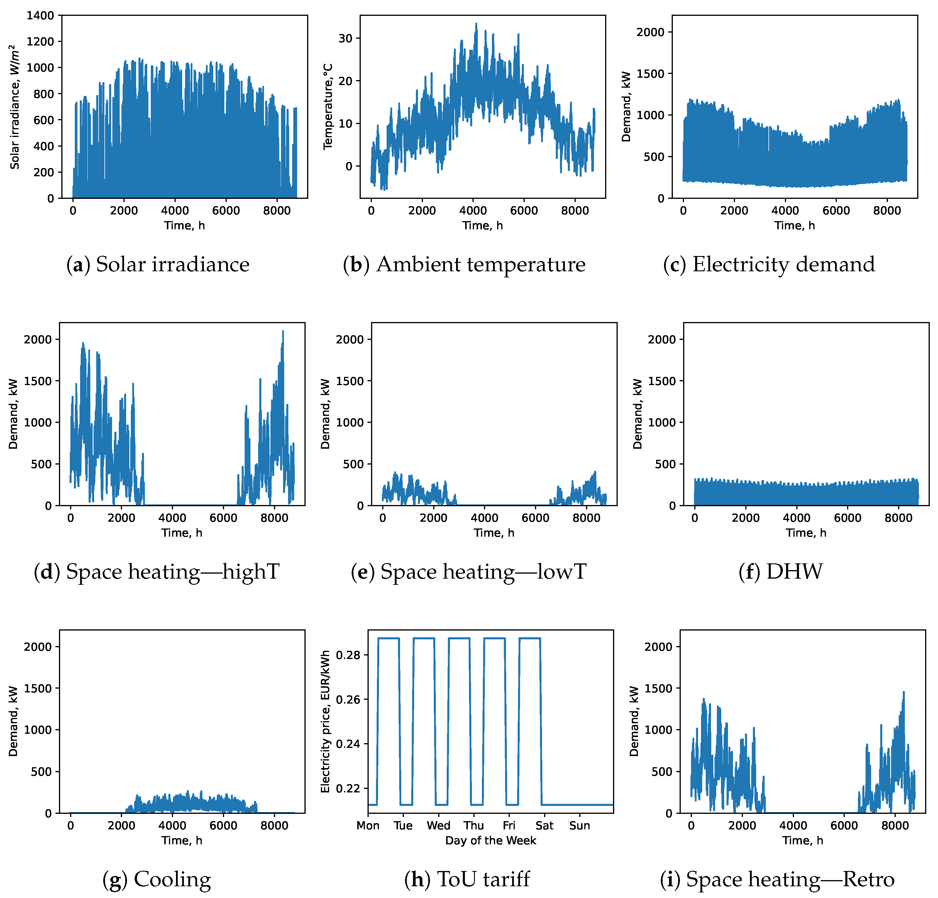
• Retro. In addition to the Flex scenario, this approach involved retrofitting the building envelopes of older structures. According to the report by EU Smart Cities Information System (SCIS) [49], and data provided by TABULA [50], after the retrofits, space heating energy needs for the older buildings were assumed to drop by 50% and could be met by a low-temperature heating network (50/40 °C). The spacing heating demands after retrofit is shown in Figure A1i.

The main parameters of the technologies, derived from the literature, are presented in Table A1–Table A4.

3. Results

This section presents the main findings from applying the modeling framework to the case study. First, an overview of the economic-environmental trade-offs for the different scenarios is provided in Section 3.1. The optimal design and operation of PED points are presented in Section 3.2. A sensitivity analysis is discussed in Section 3.3.

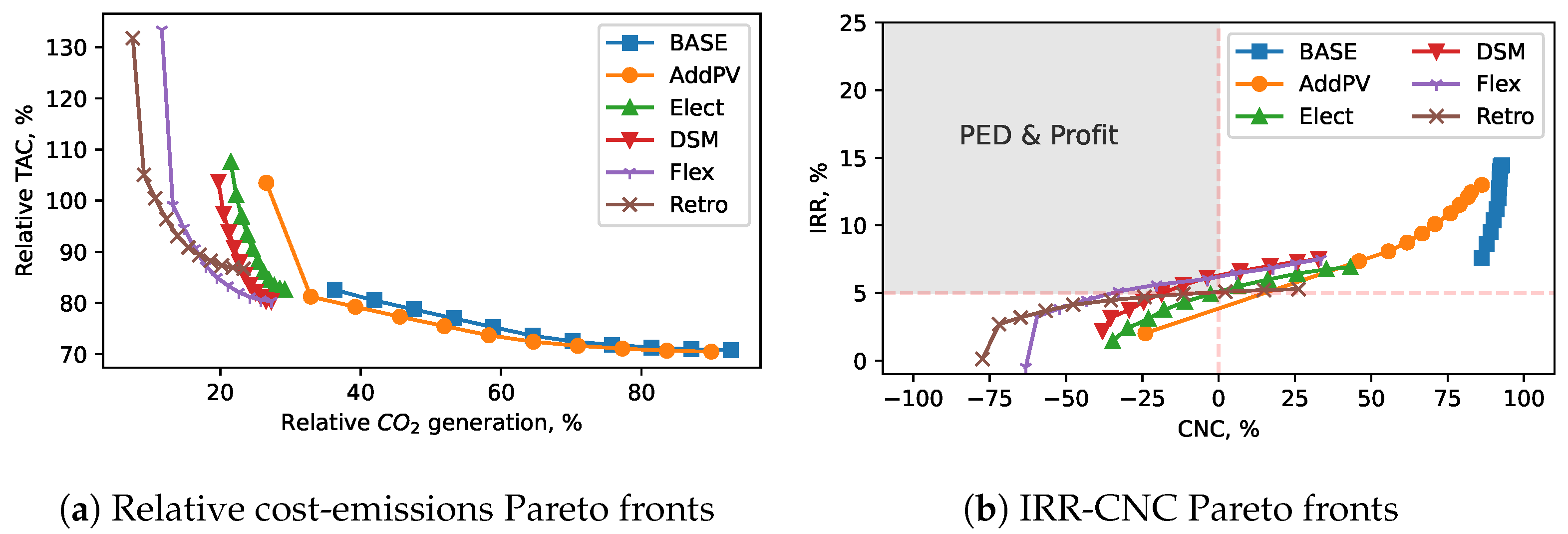
3.1. Results of Pareto Fronts

Figure 4 presents the optimal Pareto fronts for all selected scenarios, highlighting the trade-off between total annual costs and $\mathrm{C}{\mathrm{O}}_2$ emissions (Figure 4a), as well as two main KPIs: IRRs and CNC (Figure 4b). In Figure 4a, they are compared to the Business-As-Usual (BAU) scenario, which has a total annual cost (TAC) of 1701k EUR/year and carbon emissions of 1511 ton/year. To provide a clearer understanding of the cost structures associated with varying $\mathrm{C}{\mathrm{O}}_2$ emission levels, Figure 5 provides a detailed breakdown of the cost contributions for each scenario along the Pareto fronts, as presented in subfigures (a) to (f). Several vital observations emerge:

Figure 4. Pareto fronts for the selected scenarios visualizing (a) total annual costs and carbon emissions, expressed relatively to the BAU scenario; in the BAU scenario, the TAC was 1701k EUR/year with carbon emissions 1511 ton/year. (b) IRRs and CNC. The gray area shows the solutions achieved PEDs and project profitability.

Figure 5. Cost–emissions Pareto fronts for the selected scenarios. The colored areas illustrate the cost contribution of different categories. The PED points are indicated as dashed lines.

First, in the BASE scenario, significant emissions reductions could be achieved by reducing the use of fossil fuels (Figure 5a). At the CO₂-optimal point (Figure 4a), compared to the BAU scenario, emissions could be reduced by 64%, with an 18% reduction in TAC. However, due to limited local renewable energy resources, the CNC reached up to 80% (Figure 4b), indicating a continued dependency on external energy resources that an export of renewable energy could not compensate. Thus, achieving carbon neutrality (in the sense of the CNC) was not feasible in the BASE scenario.

Second, in the AddPV scenario, along the trade-off curve, only the CO₂-optimal point achieved carbon neutrality but with a sharp cost increase (Figure 4a), and an IRR of 2%, which was lower than the interest rate of 5% (Figure 4b). While increased PV capacity enabled carbon neutrality, it incurred high costs, reducing project profitability.

Next, in the Elect scenario, by excluding fossil fuel-based units, significant carbon emissions savings were possible. Even at the cost-optimal point, the CNC was reduced to 43% (Figure 4b). Compared to the BAU scenario, $\mathrm{C}{\mathrm{O}}_2$ emissions could be reduced by 71% with 20% lower costs (Figure 4a). Along the path to the emissions objective, the CNC became negative after the sixth point (Figure 4b). At the $\mathrm{C}{\mathrm{O}}_2$-optimal point, a 79% emissions reduction was achieved with 10% higher costs. These results indicate that renewable-based electrification has a high potential to achieve PEDs, aligning with reports suggesting that to meet the European climate neutrality target, electrification in the EU should increase from 50% to 70% by 2050 [51].

In the DSM scenario, incorporating demand-side management, both carbon emissions and costs were slightly reduced compared to the Elect scenario. For instance, emissions were reduced by 9% and costs by 4% at the optimal CO2 point. TOU tariffs encouraged load shifting to off-peak periods, reducing grid stress and increasing the share of renewable energy.

Shifting to the Flex scenario, which included battery storage, further reductions in carbon emissions and costs were observed along the Pareto fronts (excluding the emission-optimal point). Battery storage helped balance the mismatch between RES production and energy consumption by storing surplus renewable electricity during peak production and using it during off-peak hours. This reduced the cost of electricity, as transport costs and taxes were saved, as well as the associated $\mathrm{C}{\mathrm{O}}_2$ emissions.

Finally, retrofitting allowed for substantial emissions reductions but also resulted in higher costs. For instance, at the cost-optimal point, emissions in the Retro scenario were 15% lower than in the Flex scenario, but expenses were 8% higher. Interestingly, for achieving deeper carbon emissions reductions—less than 14% of the BAU scenario—the retrofitting approach proved more profitable than the Flex scenario. Finally, carbon emissions could be reduced by 93% with a 30% increase in costs.

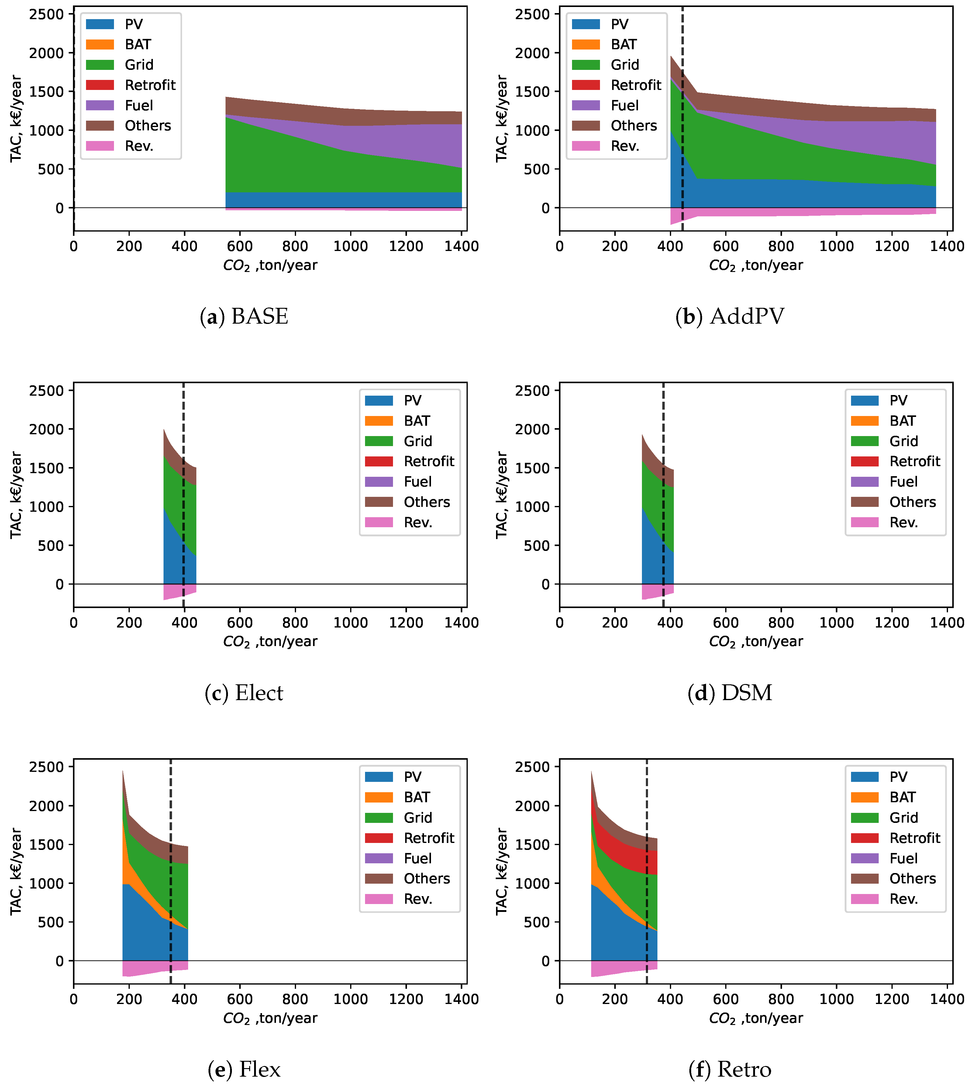
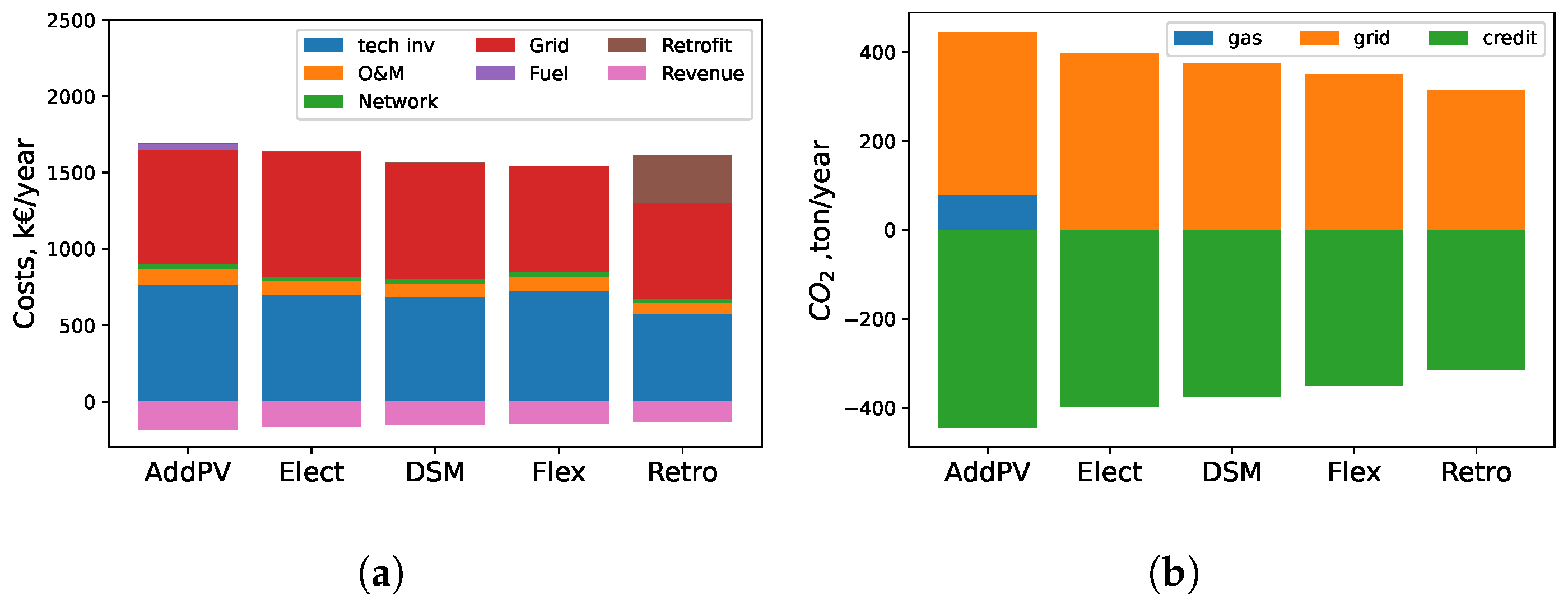
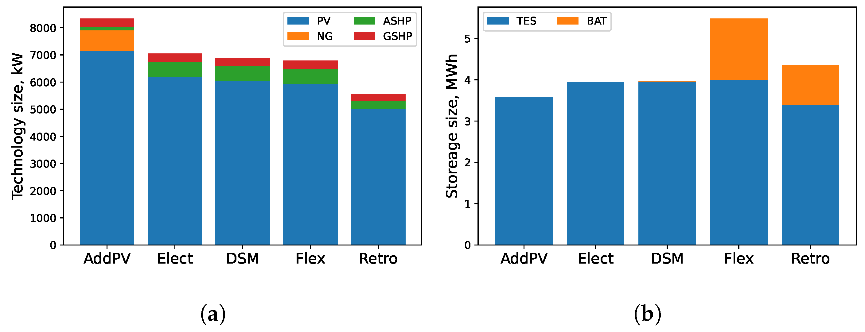
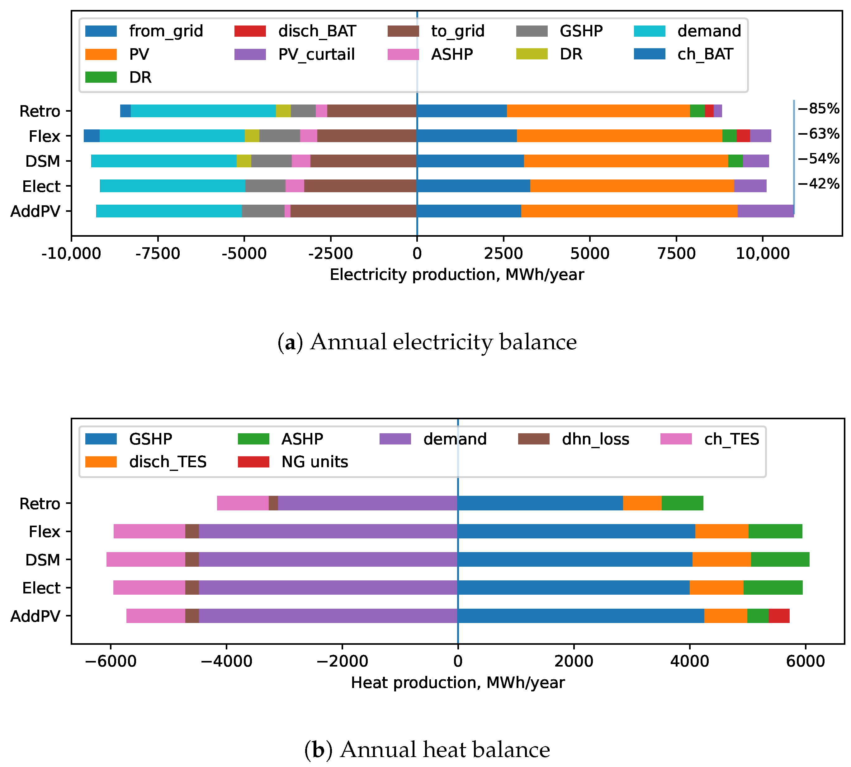
3.2. Optimal Strategies Towards Positive Energy Districts

This section begins with a description of the PED points and follows with a detailed analysis of the system components and operational strategies at these PED points.

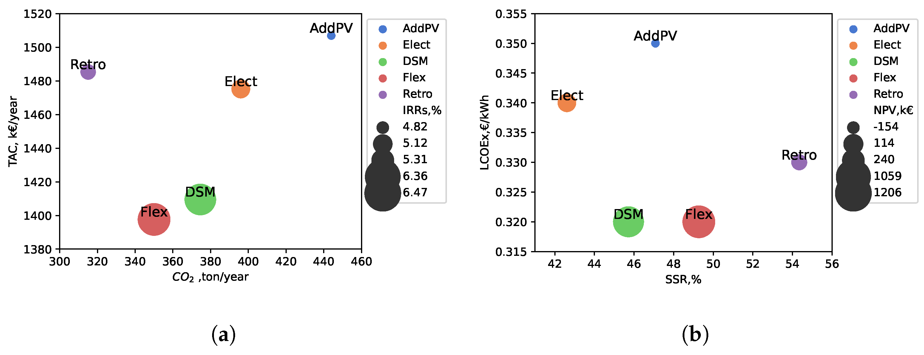
3.2.1. Definition of PED Points

For all potential PED scenarios, cases where the energy system achieved the state of PED were analyzed, further referred to as the PED points. These points represented the cost-optimal solutions with the constraint that the CNC equaled zero, i.e., that the $C{O}_2$ emissions associated with the imported energy were exactly compensated by the export of green energy, indicated as vertical lines in Figure 5. Bubble plots were used to illustrate the relationships among various PED-related parameters for different stakeholders. For instance, Figure 6 plots carbon emissions on the x-axis, the TAC on the y-axis, and IRRs are represented by bubble size. Meanwhile, Figure 6b shows the SSR on the horizontal axis and the LCOEx on the vertical axis, with the NPV illustrated by bubble size.

Figure 6. Bubble plot of KPIs for the selected scenarios at the PED points, visualizing (a) carbon emissions ($\mathrm{C}{\mathrm{O}}_2$) on the x-axis, the total annual cost (TAC) on the y-axis, and internal rate of return (IRR) as bubble size. (b) Self-Sufficiency Ratio (SSR) on the x-axis, Levelized Cost of Exergy (LCOEx) on the y-axis, and net present value (NPV) as bubble size (negative NPV indicates the scenario is not profitable).

3.2.2. Results with PED Constraint Requirements

The design results and system performance of the selected scenarios are presented in Table 3 and visualized in Figure 7 and Figure 8. The corresponding annual energy balance on a yearly basis (production and consumption), focusing on the selected scenarios, is shown in Figure 9. For a more detailed view, Figure A2 presents the monthly renewable electricity production and consumption for the AddPV scenario. The key observations that can be made based on these results are discussed below.

Table 3. Main sizing and KPIs for PED points in the selected scenarios.

Parameter	Unit	AddPV	Elect	DSM	Flex	Retro
Objectives
TAC	kEUR/year	1507	1475	1410	1398	1485
CO2	ton/year	444	396	375	350	315
Main KPIs
IRRs	%	4.8	5.3	6.4	6.5	5.1
NPV	kEUR	−155	240	1059	1206	115
LCOEx	EUR/MWh	348	337	322	317	332
SSR	%	47.1	42.6	45.7	49.3	54.3
SCR	%	32.9	38.5	42.3	46.6	48.7
Sizing results
PV	kWp	7158	6208	6049	5942	5021
BOI	kW	747	-	-	-	-
GSHP	kW	301	299	300	299	236
ASHP	kW	140	541	541	546	303
TES	MWh	3.6	3.9	4.0	4.0	3.4
BAT	MWh	-	-	-	1.5	1.0

Figure 7. The techno-economic and environmental performance for the selected scenarios at the PED points, detailed breakdown of (a) total annual costs, and (b) annual carbon emissions.

Figure 8. Technology installations for the selected scenarios at the PED points, installed capacities of (a) energy generation/conversion, (b) energy storage technologies.

Figure 9. Annual results of the energy production (+) and consumption (−), in terms of (a) annual electricity balance, (b) annual heat balance, for PED solutions with different technology configurations.

Across all PED scenarios, technology investment and electricity costs were the most significant contributors to total system costs. For example, in the Flex scenario, they accounted for 47.3% and 45.1% of the total annual cost, respectively (Figure 7a). In the Retro scenario, as expected, retrofitting led to higher investment costs, comprising 19% of the annual cost. However, this also reduced system-related costs, leading to only a slight overall cost increase of approximately 6% compared to the Flex scenario, as shown in Table 3. It is noteworthy that network costs remained very low (30k EUR/year), representing just 1.5–2% of total costs due to the minimal network length required (1300 m) to connect all buildings within the district.

Figure 7b shows the carbon emission breakdown for all the selected scenarios. Notably, in the AddPV scenario, NG-based carbon emissions accounted for 18% of the total emissions, despite natural gas contributing only 11% of total energy imports (Figure 9a). This suggests a need for greater renewable electricity production to offset emissions from fossil fuels. Variations in national emission factors for electricity, such as Belgium’s grid emission factor of 107 g/kWh in 2023 [52], compared to the NG emission factor of 202 g/kWh used in this study, highlight the potential for emissions reduction through electrification. Similar findings by Gabrielli et al. [53] support this, showing that lower grid emissions can reduce dependence on decentralized generation and storage technologies.

Meeting PED targets necessitated additional PV capacity in all scenarios. The AddPV scenario required the highest PV capacity of 7158 kWp, compared to the current maximum of 2103 kWp. Although overall renewable electricity generation (7879 MWh) exceeded annual consumption (5256 MWh), grid exchange limits and mismatches between production and consumption (daily and monthly, as shown in Figure A2) resulted in a low self-consumption ratio of 32.9% and significant PV curtailment of about 1620 MWh/year (Figure 9a). This underscores the need for technologies to manage renewable energy fluctuations.

Renewable-based electrification showed significant potential for achieving PEDs. The Elect scenario, which used electric heat pumps for primary heating, reduced both costs and $C{O}_2$ emissions. It increased energy efficiency, raising the SCR to 38.5% and reducing PV curtailment by 42% compared to the AddPV scenario (Figure 9a).

Demand response (DR) is vital for progressing toward PED. In the DSM scenario, DR balanced peak loads by 419.12 MWh, enabling better integration of renewable energy sources. This resulted in a 54% reduction in PV curtailment and a 177 MWh decrease in grid electricity imports.

Battery storage enhanced energy flexibility further. In the Flex scenario, the system benefited from 391.03 MWh of discharged battery energy, aiding peak load management and improving energy flexibility. As expected, the Flex scenario also achieved significant reductions in both PV curtailment (602.59 MWh) and grid imports (203 MWh) through improved energy management and storage solutions.

Retrofitting focuses on reducing energy demand rather than solely maximizing PV capacity. The Retro scenario achieved a 30% reduction in heat demand, resulting in the lowest $C{O}_2$ emissions (315 tons/year), the lowest PV capacity (5021 kWp), the highest SCR (48.7%), and minimal PV curtailment (233.78 MWh).

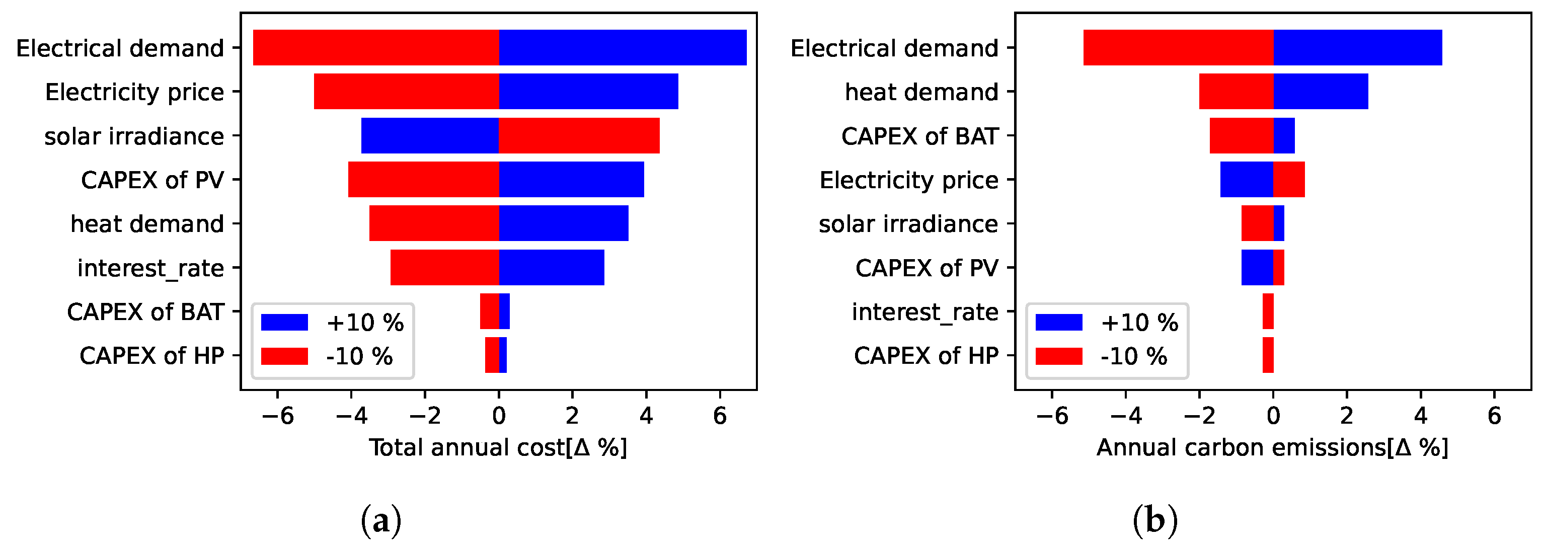
3.3. Sensitivity Analysis

To evaluate the impact of key input parameters on cost and carbon emissions at the PED points, a sensitivity analysis was conducted for the optimal PED points of the Flex Scenario. The selected parameters included electricity price, electricity and heat demand, CAPEX of PV panels, battery storage, heat pumps, solar irradiance, and interest rate. Each parameter was individually varied by ±10% to assess its effect on system performance.

Figure 10 shows that electricity demand had the biggest impact on both costs and carbon emissions (±6–8% for ±10% change). This was anticipated as higher demand increases energy consumption, driving up expenses and emissions. Similarly, heat demand significantly influenced both metrics (±5–7% impact), reflecting the energy-intensive nature of heating requirements. Electricity price strongly influenced costs (±5% variation) but had no direct effect on carbon emissions, as grid prices affect total expenses without altering the energy mix. Solar irradiance and PV CAPEX significantly impacted costs (around ±4% variation) but had a limited effect on emissions due to PV curtailment (Figure 9a). The interest rate was also a notable factor affecting costs (±3% variation), driven by the high capital investment in system components (Figure 7). Other CAPEX parameters, such as battery storage and heat pumps, showed minimal sensitivity (less than ±0.5%), as the majority of the investment in this case study was allocated to PV panels (Figure 5).

Figure 10. Tornado plots with Retro scenario, for the sensitivity of model results on (a) total annual cost and (b) annual carbon emissions, when selected parameters were increased and decreased by 10%.

Additionally, Figure 11 explores the sensitivity of the grid share to electricity price, and installed capacities relative to the baseline average price (245.3 EUR/MWh). Figure 11a shows that the grid share declined as the electricity price rose, due to the installation of more batteries and the increased storage of surplus PV energy in these batteries instead of curtailing it. Conversely, when the electricity price fell below approximately 150 EUR/MWh, no batteries were installed, and reliance on grid electricity grew, with grid share peaking at 38% when the electricity price was 0 EUR/MWh, highlighting the critical role of dynamic pricing policies in stabilizing PED economics.

Figure 11. Impact of varying electricity prices on grid demand and installed technology capacities in the Flex scenario: (a) electricity supplied by the grid, (b) relative installed capacities (baseline = 245.3 EUR/MWh).

4. Discussion and Limitations

In this section, the main contributions of the evaluation model for pre-designing PEDs, based on the previous results, are discussed. Additionally, the limitations of the model and the methodology used for evaluating PEDs are addressed.

4.1. Discussions of Technical Solutions to PEDs

The PED pre-design framework introduced in this study offers a straightforward yet effective method for comparing and visualizing pathways to PEDs. Given that PEDs require collaboration among multiple stakeholders during the design process, this model facilitates a comprehensive assessment of optimal deployment strategies. By integrating the various pillars of the PED energy system, this iterative process generates diverse solutions with varying evaluation metrics, ultimately guiding the design to meet both PED targets and stakeholder expectations [7,54].

The case study demonstrated that expanding the capacity of renewable energy sources (RES) was crucial for PEDs in densely populated areas. As illustrated in Figure 8a, achieving PED targets necessitated a 2.4 to 3.4 times greater PV capacity than the available roof area. This finding is consistent with Guarino et al. [6]. Additional strategies to meet these targets include utilizing virtual renewable resources, integrating Building-Integrated PV (BIPV) [21,28], leasing renewable energy units, or forming energy cooperatives [54].

The results underscore the importance of deep electrification. As shown in Figure 4a, renewable-based electrification can achieve carbon emissions reductions of 71–79%. This aligns with recent studies [55,56] and the World Energy Transitions Outlook [57], which highlight electrification and energy efficiency as critical drivers for meeting the 1.5 °C target by 2050.

Demand-side management (DSM) is another effective strategy, encouraging customers to reduce peak loads through price incentives. Tariff structures like the capacity tariff, implemented in Flanders since 2023, which charges prices based on the highest electricity usage at any one time [58], are vital and should be adapted to future energy structures.

Battery storage plays a crucial role in enhancing energy efficiency and achieving deep decarbonization. As shown in Figure 5e,f, battery storage capacity increased with carbon emissions savings, reaching 1–1.5 MWh to achieve PEDs (Table 3). However, to achieve deep decarbonization, such as reducing emissions below 150 tons/year in the Retro scenario (Figure 5f), higher battery storage was required, consistent with findings by Marocco et al. [34]. Additionally, achieving climate neutrality by 2050 may necessitate more advanced and costly technologies like power-to-hydrogen (PtH2) systems [34,59]. Since the study focused on current technologies, future solutions like hydrogen-based systems were excluded. For a discussion on hydrogen’s role in achieving zero emissions, the reader is referred to our previous work [30].

While retrofitting may not be the most economically profitable solution, it provides a balanced approach, providing both environmental and economic benefits. Some researchers advocate retrofitting as the primary strategy in the transition to PEDs in Europe [5,27]. This study considered only retrofit-related costs, excluding potential subsidies or increased building value post-retrofit, which could improve the net present value (NPV) and internal rates of return (IRRs). Local authorities are also crucial in facilitating the PED transition. In Flanders, energy performance certificate (PEC) ratings are required to improve from level E to B by 2035 [60], highlighting the need for fair distribution of responsibilities and benefits among stakeholders and regional financing plans [54].

In this case study, the heat network, extending about 1300 m, accounted for only 5% of the heat loss. Notably, in the Retro scenario, heat network loss was reduced by 30%, from 235 MWh/year to 162 MWh/year. Low-temperature heating solutions become increasingly important for longer pipelines with higher heat losses.

4.2. Limitations

The operational modeling of energy conversion units in this study was simplified. Vital operational features—such as part-load efficiencies, investment curves, ramping rates, start-up costs, and degradation curves—were not considered, as they require more complex computations [61].

Next, several works offer insights into economic incentives for shared electricity that encourage citizen engagement [62,63,64]. However, these incentives, as outlined by the revised Energy Efficiency Directive (EU/2023/1791) [65], were not accounted for in this model.

Additionally, several parameters, including electricity tariffs, $\mathrm{C}{\mathrm{O}}_2$ taxes, grid exchange limits, retrofit subsidies, and weather conditions, are subject to change. However, this study focused on presenting evaluation metrics and did not address the uncertainty of these parameters or their impact on PED performance.

Moreover, this study concentrated on the techno-economic and environmental analysis of the proposed system as a pathway to PED development. Although social and political criteria (e.g., energy justice [10], financial feasibility, and stakeholder acceptance) are critical challenges for PED implementation [7], these aspects are being addressed within the scope of the Citizens4PED project but were not included in this study.

Finally, while this study focused primarily on discussing potential solutions to achieve PED targets within the scope of a specific case study, the exploration of the PED concept in different climatic regions [24] is considered as future work and was not implemented in this study.

5. Conclusions and Future Work

This study presented a comprehensive framework for the pre-design of Positive Energy Districts (PEDs) through multi-objective optimization, integrating techno-economic and environmental analyses. The framework integrated various technical solutions, including renewable energy sources (RESs), electrification, demand-side management (DSM), battery storage, and retrofitting, and evaluated them against key performance indicators (KPIs) such as the Carbon Neutrality Check (CNC) and internal rate of return (IRR).

The case study results demonstrated that expanding renewable energy capacities, mainly through photovoltaic (PV) systems, was a critical first step in achieving the PED targets. For example, in scenarios with increased PV capacity, the renewable-based electrification approach achieved up to 79% carbon emissions reduction.

Battery storage played a pivotal role in balancing energy supply and demand, with scenarios including battery storage showing significant reductions in both PV curtailment and grid imports. Additionally, integrating DSM strategies helped smooth peak loads, enhancing the system’s efficiency and reducing grid dependency. Retrofitting existing buildings, while not the most economically profitable solution, provided a balanced approach that effectively reduced overall energy demand and emissions, achieving the lowest $C{O}_2$ emissions of 315 tons/year with the highest self-consumption ratio (SCR) of 48.7%.

The framework optimizes economic and environmental outcomes and presents various solutions to stakeholders, helping them identify final design options that accommodate their diverse perspectives. This approach facilitates more informed decision-making, ensuring the final PED design aligns with sustainability goals and stakeholder interests.

Future research should consider multi-stage investment strategies, enabling greater flexibility in decision-making and long-term planning [37]. Additionally, the framework can be significantly improved by incorporating the Polynomial Chaos Expansion (PCE) algorithm for uncertainty quantification analysis [42] and integrating life-cycle assessment methods [14] to provide a comprehensive evaluation of environmental impacts. Moreover, future work should explore targeted policy interventions and economic incentives—such as subsidies, tax incentives, and shared electricity programs—to encourage citizen engagement and fully capture the potential benefits of these incentives within the framework.

Appendix A.1. System Components

Appendix A.1.1. PV Array

The electrical power generated by the PV array can be computed as follows [66]:

$$P_{\mathrm{PV},d,t}=A_{\mathrm{PV}}·{\eta }_m·K_T·K_f·G_{\mathrm{sol},d,t}\forall d\in \mathrm{D},t\in \mathrm{T}$$

(A4)

where $P_{\mathrm{PV}}$ represents the output power of the PV array, $A_{\mathrm{PV}}$ is the total area of the PV array, $G_{\mathrm{sol}}$ is solar irradiation, ${\eta }_m$ represents the conversion efficiency under the standard test condition (%), and $K_{\mathrm{f}}$ is the correction coefficient except temperature.

Appendix A.1.2. BOI

The boiler can generate heat by using fuel, and the outputs of the BOI are depicted as follows:

$$Q_{\mathrm{BOI},d,t}=Fue{l}_{\mathrm{BOI},d,t}·{\eta }_{\mathrm{BOI}}^{\mathrm{heat}}\forall d\in \mathrm{D},t\in \mathrm{T}$$

(A5)

where $Q_{\mathrm{BOI}}$ represents the output heat of the BOI. $Fue{l}_{\mathrm{BOI}}$ is the fuel requirement of the BOI.

Appendix A.1.3. CHP

The CHP can generate both heat and electricity, and the outputs of the CHP are depicted as follows:

$$\begin{array}{cccc}\hfill Q_{\mathrm{CHP},d,t}& =Fue{l}_{\mathrm{CHP},d,t}·{\eta }_{\mathrm{CHP}}^{\mathrm{heat}}\hfill & \hfill & \forall d\in \mathrm{D},t\in \mathrm{T},\hfill \end{array}$$

(A6)

$$\begin{array}{cccc}\hfill P_{\mathrm{CHP},d,t}& =Fue{l}_{\mathrm{CHP},d,t}·{\eta }_{\mathrm{CHP}}^{\mathrm{elec}}\hfill & \hfill & \forall d\in \mathrm{D},t\in \mathrm{T}.\hfill \end{array}$$

(A7)

where $Q_{\mathrm{CHP}}$ and $P_{\mathrm{CHP}}$ represent the output heat and electricity of the CHP, respectively. $Fue{l}_{\mathrm{CHP}}$ is the fuel requirement of the CHP.

Appendix A.1.4. Heat Pump

A heat pump is used to generate heat using electricity, and the output of the heat pump is described as follows:

$$Q_{\mathrm{HP},d,t}=P_{\mathrm{HP},d,t}·{\mathrm{COP}}_{\mathrm{HP},d,t}\forall d\in \mathrm{D},t\in \mathrm{T}$$

(A8)

To model the heat pump, the coefficient of performance (COP) is employed based on the Carnot efficiency [67],

$${\mathrm{COP}}_{\mathrm{HP}}={\eta }_{\mathrm{Carnot}}·{\mathrm{COP}}_{\mathrm{Carnot}}={\eta }_{\mathrm{Carnot}}·{\displaystyle \frac{T_{\mathrm{sink}}}{T_{\mathrm{sink}}-T_{\mathrm{source}}}}$$

(A9)

where ${\eta }_{\mathrm{Carnot}}$ is the Carnot efficiency as the ratio between the actual and Carnot coefficients of performance. $T_{\mathrm{sink}}$ and $T_{\mathrm{source}}$ are the condensing temperature and evaporating temperature of the refrigerant, respectively. As described in [67], for each heat transfer, a minimal temperature difference $\mathrm{\Delta }{T}^{\min }$ between the two sides of the heat exchanger is considered. In the case of water-to-water heat transfer, $\mathrm{\Delta }{T}^{\min }$ = 2 $\mathrm{K}$. In the case of water-to-air heat transfer, $\mathrm{\Delta }{T}^{\min }$ = 10 $\mathrm{K}$.

Appendix A.2. Energy Storage

The approaches by Gabriell et al. [53] and Wirtz et al. [61] were used for seasonal storage modeling. The association between the original days y ∈ Y= {1,2,...,365} and the design days d $\in \mathrm{D}$ is the sequence $\sigma$ of design days. Further details on the seasonal energy storage modeling are presented in our previous work [30].

The state of charge is expressed as:

$$\begin{array}{cc}\hfill S_{k,y,t}& =S_{k,y,t-1}+P_{k,\sigma \left(y\right),t}^{\mathrm{ch}}·{\eta }_k^{\mathrm{ch}}-{\displaystyle \frac{P_{k,\sigma \left(y\right),t}^{\mathrm{dch}}}{{\eta }_k^{\mathrm{dch}}}}\hfill \\ \hfill \forall k& \in \{\mathrm{BAT},\mathrm{TES}\},y\in \mathrm{Y},t\in \mathrm{T}.\hfill \end{array}$$

(A10)

The state of charge is limited by:

$$\begin{array}{cc}\hfill S_k^{\mathrm{cap}}·s_k^{\min }& \le S_{k,y,t}\le S_k^{\mathrm{cap}}·s_k^{\max }\hfill \\ \hfill \forall k& \in \{\mathrm{BAT},\mathrm{TES}\},y\in \mathrm{Y},t\in \mathrm{T}.\hfill \end{array}$$

(A11)

The maximum capacity limits the storage capacities.

$$S_k^{\mathrm{cap}}\le S_k^{\max }\forall k\in \{\mathrm{BAT},\mathrm{TES}\}.$$

(A12)

The charging and discharging power are limited by the minimum charging and discharging time $\tau$, respectively. A special ordered set 1 (SOS1) constraint is also applied [68,69], which ensures that for each time step, at most one variable in the on/off status set {${\zeta }_{k,d,t}^{\mathrm{ch}}$, ${\zeta }_{k,d,t}^{\mathrm{dch}}$} is non-zero.

$$\begin{array}{cccc}\hfill P_{k,d,t}^{\mathrm{ch}}& \le {\displaystyle \frac{S_k^{\mathrm{cap}}}{{\tau }_k}}\hfill & \hfill & \forall k\in \{\mathrm{BAT},\mathrm{TES}\},d\in \mathrm{D},t\in \mathrm{T},\hfill \end{array}$$

(A13)

$$\begin{array}{cccc}\hfill P_{k,d,t}^{\mathrm{dch}}& \le {\displaystyle \frac{S_k^{\mathrm{cap}}}{{\tau }_k}}\hfill & \hfill & \forall k\in \{\mathrm{BAT},\mathrm{TES}\},d\in \mathrm{D},t\in \mathrm{T},\hfill \end{array}$$

(A14)

$$\begin{array}{cccc}\hfill \sum _{i\in \{\mathrm{ch},\mathrm{dch}\}}{\zeta }_{k,d,t}^i& \le 1\hfill & \hfill & \forall k\in \{\mathrm{BAT},\mathrm{TES}\},d\in \mathrm{D},t\in \mathrm{T}.\hfill \end{array}$$

(A15)

where $S_{k,y,t}$ is the amount of energy stored in the storage unit k at time step t of original day y. $S_k^{\mathrm{cap}}$ is the storage capacity of the storage unit k. $P_k^{\mathrm{ch}}$ and $P_k^{\mathrm{dch}}$ represent the charge and discharge energy flows of storage unit k, respectively. ${\eta }_k^{\mathrm{ch}}$ and ${\eta }_k^{\mathrm{dch}}$ are the charge and discharge efficiency of storage unit k, respectively. ${\zeta }_{k,d,t}^i$ are the binary variables of those units characterized by an on/off status.

Appendix A.3. Energy Balance

To meet the energy demand of the community, the energy balances for electricity, heating, and cooling are expressed as follows.

For electricity, the power supply includes power imported from the grid, generation by the PV array, CHP, and discharging of the battery. The power demand encompasses electricity demand, power consumed by each heat pump, charging of the battery, and power export to the grid. This is illustrated by

$$\begin{array}{cc}\hfill P_{\mathrm{PV},d,t}& +P_{\mathrm{CHP},d,t}+P_{\mathrm{grid},d,t}^{\mathrm{import}}+P_{\mathrm{BAT},d,t}^{\mathrm{dch}}\hfill \\ \hfill & =P_{\mathrm{dem},d,t}+P_{\mathrm{HP},d,t}+P_{\mathrm{BAT},d,t}^{\mathrm{ch}}+P_{\mathrm{grid},d,t}^{\mathrm{export}}\forall d\in \mathrm{D},t\in \mathrm{T}\hfill \end{array}$$

(A16)

On the heating side, the demand includes domestic hot water (DHW), high-temperature space heating ($sh\_ht$), low-temperature space heating ($sh\_lt$). For the high-temperature heat balance, the heat supply includes heat generated by the CHP, BOI, high-temperature GSHP and ASHP, and discharging of the TES. The heat demands include the required heat load and the charging of the TES:

$$\begin{array}{cc}\hfill & Q_{\mathrm{ASHP},d,t}+Q_{\mathrm{CHP},d,t}+Q_{\mathrm{BOI},d,t}+Q_{\mathrm{TES},d,t}^{\mathrm{dch}}\hfill \\ \hfill & =Q_{\mathrm{dem},d,t}^{\mathrm{dhw}}+Q_{\mathrm{dem},d,t}^{\mathrm{sh}\_\mathrm{ht}}+Q_{\mathrm{TES},d,t}^{\mathrm{ch}}\forall d\in \mathrm{D},t\in \mathrm{T}\hfill \end{array}$$

(A17)

For the low-temperature heat balance, the heat supply includes heat generated by the low-temperature heat pump and GSHP and the discharging of the TES. The heat demands include the required heat load and the charging of the TES:

$$\begin{array}{cc}\hfill & Q_{\mathrm{GSHP},d,t}+Q_{\mathrm{TES},d,t}^{\mathrm{dch}}=Q_{\mathrm{dem},d,t}^{\mathrm{sh}\_\mathrm{lt}}+Q_{\mathrm{TES},d,t}^{\mathrm{ch}}\forall d\in \mathrm{D},t\in \mathrm{T}\hfill \end{array}$$

(A18)

The cooling energy balance is illustrated as follows:

$$Q_{c,\mathrm{HEX},d,t}=Q_{c,\mathrm{dem},d,t}\forall d\in \mathrm{D},t\in \mathrm{T}$$

(A19)

Appendix A.4. Constraints

Appendix A.4.1. Minimum Part Load

Many technical devices cannot operate in any low part load; therefore, according to Wirtz et al. [69], minimum part-load limitations for thermal energy conversion technologies were considered in this model.

$$\begin{array}{cc}\hfill {\mathrm{PLR}}_k·Q_k^{\mathrm{norm}}& \le Q_{k,d,t}+\widehat{M}\left(1-y_{k,d,t}\right)\hfill \\ \hfill & \forall k\in \{\mathrm{BOI},\mathrm{ASHP},\mathrm{GSHP}\},d\in \mathrm{D},t\in \mathrm{T}.\hfill \end{array}$$

(A20)

where ${\mathrm{PLR}}_k$ is the minimum part-load ratio of technology k. $y_{k,d,t}$ are the binary variables, indicating if a technology k is running at a certain time step ($y_{k,d,t}$ =1) or not ($y_{k,d,t}$ = 0). Here, a big-M constraint was used according to the literature [69] to ensure the output of a component was zero if the part-load ratio was smaller than the minimum part-load ratio.

Appendix A.4.2. Demand Response Program

The demand response program’s role is to reduce the overall costs by varying the load consumption patterns; the time-of-use (TOU) rate of demand response program (DPR) was considered in this study. The load curve over a defined time horizon was changed by shifting a certain percentage of load from one period to another period based on the price of energy carriers [70]. The new electrical load thus became equal to the base load plus a variable power term, which could be either positive or negative [71].

$$P_{\mathrm{dem},\mathrm{DRP},d,t}=P_{\mathrm{dem},d,t}+P_{\mathrm{dem},d,t}^{\mathrm{TOU}}\forall d\in \mathrm{D},t\in \mathrm{T}$$

(A21)

The amount of the load shaving should be less than a certain ratio of the base load (${\mathrm{DPR}}^{max}$), which can be expressed as:

$$-P_{\mathrm{dem},d,t}·{\mathrm{DPR}}^{max}\le P_{\mathrm{dem},d,t}^{\mathrm{TOU}}\le P_{\mathrm{dem},d,t}·{\mathrm{DPR}}^{max}\forall d\in \mathrm{D},t\in \mathrm{T}$$

(A22)

As the DRP mechanism is just a translation of a certain amount of load from some periods to others to achieve a cost reduction, the overall load over a certain time ($T_{\mathrm{DPR}}$) remains fixed, as described by the following constraint:

$$\sum _{t=1}^{T_{\mathrm{DPR}}}{P}_{\mathrm{dem},d,t}^{\mathrm{TOU}}=0\forall d\in \mathrm{D}$$

(A23)

References

- IEA. Empowering Cities for a Net Zero Future: Unlocking Resilient, Smart, Sustainable Urban Energy Systems; International Energy Agency (IEA): Paris, France, 2021; Available online: https://www.iea.org/reports/empowering-cities-for-a-net-zero-future/ (accessed on 20 February 2025).
- Bruck, A.; Díaz Ruano, S.; Auer, H. A Critical Perspective on Positive Energy Districts in Climatically Favoured Regions: An Open-Source Modelling Approach Disclosing Implications and Possibilities. Energies 2021, 14, 4864. [Google Scholar] [CrossRef]
- SET-Plan Working Group. Europe to become a global role model in integrated, innovative solutions for the planning, deployment, and replication of Positive Energy Districts. SET-Plan Action 2018, 32, 1–72. Available online: https://jpi-urbaneurope.eu/wp-content/uploads/2021/10/setplan_smartcities_implementationplan-2.pdf (accessed on 20 February 2025).
- Hinterberger, R.; Gollner, C.; Noll, M.; Meyer, S.; Schwarz, H.G. Reference Framework for Positive Energy Districts and Neighbourhoods; JPI Urban Europe: Wien, Austria, 2020; Available online: https://jpi-urbaneurope.eu/wp-content/uploads/2020/04/White-Paper-PED-Framework-Definition-2020323-final.pdf (accessed on 20 February 2025).
- Sassenou, L.N.; Olivieri, L.; Olivieri, F. Challenges for positive energy districts deployment: A systematic review. Renew. Sustain. Energy Rev. 2024, 191, 114152. [Google Scholar] [CrossRef]
- Guarino, F.; Rincione, R.; Mateu, C.; Teixidó, M.; Cabeza, L.F.; Cellura, M. Renovation assessment of building districts: Case studies and implications to the positive energy districts definition. Energy Build. 2023, 296, 113414. [Google Scholar] [CrossRef]
- Sassenou, L.N.; Olivieri, F.; Civiero, P.; Olivieri, L. Methodologies for the design of positive energy districts: A scoping literature review and a proposal for a new approach (PlanPED). Build. Environ. 2024, 260, 111667. [Google Scholar] [CrossRef]
- Lindholm, O.; Rehman, H.u.; Reda, F. Positioning Positive Energy Districts in European Cities. Buildings 2021, 11, 19. [Google Scholar] [CrossRef]
- Natanian, J.; Guarino, F.; Manapragada, N.; Magyari, A.; Naboni, E.; De Luca, F.; Cellura, S.; Brunetti, A.; Reith, A. Ten questions on tools and methods for positive energy districts. Build. Environ. 2024, 255, 111429. [Google Scholar] [CrossRef]
- Casamassima, L.; Bottecchia, L.; Bruck, A.; Kranzl, L.; Haas, R. Economic, social, and environmental aspects of Positive Energy Districts—A review. WIREs Energy Environ. 2022, 11, e452. [Google Scholar] [CrossRef]
- Gabaldón Moreno, A.; Vélez, F.; Alpagut, B.; Hernández, P.; Sanz Montalvillo, C. How to Achieve Positive Energy Districts for Sustainable Cities: A Proposed Calculation Methodology. Sustainability 2021, 13, 710. [Google Scholar] [CrossRef]
- Bruck, A.; Diaz Ruano, S.; Auer, H. Values and implications of building envelope retrofitting for residential Positive Energy Districts. Energy Build. 2022, 275, 112493. [Google Scholar] [CrossRef]
- Volpe, R.; Gonzalez Alriols, M.; Martelo Schmalbach, N.; Fichera, A. Optimal design and operation of distributed electrical generation for Italian positive energy districts with biomass district heating. Energy Convers. Manag. 2022, 267, 115937. [Google Scholar] [CrossRef]
- Marrasso, E.; Martone, C.; Pallotta, G.; Roselli, C.; Sasso, M. A novel methodology and a tool for supporting the transition of districts and communities in Positive Energy Districts. Energy Build. 2024, 318, 114435. [Google Scholar] [CrossRef]
- Sareen, S.; Albert-Seifried, V.; Aelenei, L.; Reda, F.; Etminan, G.; Andreucci, M.B.; Kuzmic, M.; Maas, N.; Seco, O.; Civiero, P.; et al. Ten questions concerning positive energy districts. Build. Environ. 2022, 216, 109017. [Google Scholar] [CrossRef]
- Andresen, I.; Healey Trulsrud, T.; Finocchiaro, L.; Nocente, A.; Tamm, M.; Ortiz, J.; Salom, J.; Magyari, A.; Hoes-van Oeffelen, L.; Borsboom, W.; et al. Design and performance predictions of plus energy neighbourhoods—Case studies of demonstration projects in four different European climates. Energy Build. 2022, 274, 112447. [Google Scholar] [CrossRef]
- Salom, J.; Tamm, M.; Andresen, I.; Cali, D.; Magyari, A.; Bukovszki, V.; Balázs, R.; Dorizas, P.V.; Toth, Z.; Zuhaib, S.; et al. An Evaluation Framework for Sustainable Plus Energy Neighbourhoods: Moving Beyond the Traditional Building Energy Assessment. Energies 2021, 14, 4314. [Google Scholar] [CrossRef]
- Volpe, R.; Cutore, E.; Fichera, A. Design and Operational Indicators to Foster the Transition of Existing Renewable Energy Communities towards Positive Energy Districts. J. Sustain. Dev. Energy, Water Environ. Syst. 2024, 12, 1–22. [Google Scholar] [CrossRef]
- Hedman, A.; Rehman, H.U.; Gabaldón, A.; Bisello, A.; Albert-Seifried, V.; Zhang, X.; Guarino, F.; Grynning, S.; Eicker, U.; Neumann, H.M.; et al. IEA EBC Annex83 Positive Energy Districts. Buildings 2021, 11, 130. [Google Scholar] [CrossRef]
- Heller, R. Positive Energy in the City; Eburon Academic Publishers: Delft, The Netherlands, 2022; Available online: https://pure.hva.nl/ws/portalfiles/portal/23920668/positive_energy_in_the_city.pdf (accessed on 20 February 2025).
- Gouveia, J.; Seixas, J.; Palma, P.; Duarte, H.; Luz, H.; Cavadini, G. Positive Energy District: A Model for Historic Districts to Address Energy Poverty. Front. Sustain. Cities 2021, 3, 648473. [Google Scholar] [CrossRef]
- Guasselli, F.; Vavouris, A.; Stankovic, L.; Stankovic, V.; Didierjean, S.; Gram-Hanssen, K. Smart energy technologies for the collective: Time-shifting, demand reduction and household practices in a Positive Energy Neighbourhood in Norway. Energy Res. Soc. Sci. 2024, 110, 103436. [Google Scholar] [CrossRef]
- Marotta, I.; Péan, T.; Guarino, F.; Longo, S.; Cellura, M.; Salom, J. Towards Positive Energy Districts: Energy Renovation of a Mediterranean District and Activation of Energy Flexibility. Solar 2023, 3, 253–282. [Google Scholar] [CrossRef]
- Bruck, A.; Díaz Ruano, S.; Auer, H. One piece of the puzzle towards 100 Positive Energy Districts (PEDs) across Europe by 2025: An open-source approach to unveil favourable locations of PV-based PEDs from a techno-economic perspective. Energy 2022, 254, 124152. [Google Scholar] [CrossRef]
- Laitinen, A.; Lindholm, O.; Hasan, A.; Reda, F.; Hedman, Å. A techno-economic analysis of an optimal self-sufficient district. Energy Convers. Manag. 2021, 236, 114041. [Google Scholar] [CrossRef]
- Marrasso, E.; Martone, C.; Pallotta, G.; Roselli, C.; Sasso, M. Assessment of energy systems configurations in mixed-use Positive Energy Districts through novel indicators for energy and environmental analysis. Appl. Energy 2024, 368, 123374. [Google Scholar] [CrossRef]
- Blumberga, A.; Vanaga, R.; Freimanis, R.; Blumberga, D.; Antužs, J.; Krastiņš, A.; Jankovskis, I.; Bondars, E.; Treija, S. Transition from traditional historic urban block to positive energy block. Energy 2020, 202, 117485. [Google Scholar] [CrossRef]
- An, Y.S.; Kim, J.; Joo, H.J.; woo Han, G.; Kim, H.; Lee, W.; Kim, M.H. Retrofit of renewable energy systems in existing community for positive energy community. Energy Rep. 2023, 9, 3733–3744. [Google Scholar] [CrossRef]
- Bambara, J.; Athienitis, A.K.; Eicker, U. Residential Densification for Positive Energy Districts. Front. Sustain. Cities 2021, 3, 630973. [Google Scholar] [CrossRef]
- Wang, G.; Blondeau, J. Optimal combination of daily and seasonal energy storage using battery and hydrogen production to increase the self-sufficiency of local energy communities. J. Energy Storage 2024, 92, 112206. [Google Scholar] [CrossRef]
- Zheng, N.; Zhang, H.; Duan, L.; Wang, Q.; Bischi, A.; Desideri, U. Techno-economic analysis of a novel solar-driven PEMEC-SOFC-based multi-generation system coupled parabolic trough photovoltaic thermal collector and thermal energy storage. Appl. Energy 2023, 331, 120400. [Google Scholar] [CrossRef]
- Benalcazar, P. Sizing and optimizing the operation of thermal energy storage units in combined heat and power plants: An integrated modeling approach. Energy Convers. Manag. 2021, 242, 114255. [Google Scholar] [CrossRef]
- Coppieters, T.; Blondeau, J. Techno-Economic Design of Flue Gas Condensers for Medium-Scale Biomass Combustion Plants: Impact of Heat Demand and Return Temperature Variations. Energies 2019, 12, 2337. [Google Scholar] [CrossRef]
- Marocco, P.; Ferrero, D.; Lanzini, A.; Santarelli, M. The role of hydrogen in the optimal design of off-grid hybrid renewable energy systems. J. Energy Storage 2022, 46, 103893. [Google Scholar] [CrossRef]
- Coppitters, D.; Verleysen, K.; De Paepe, W.; Contino, F. How can renewable hydrogen compete with diesel in public transport? Robust design optimization of a hydrogen refueling station under techno-economic and environmental uncertainty. Appl. Energy 2022, 312, 118694. [Google Scholar] [CrossRef]
- Ma, T.; Javed, M.S. Integrated sizing of hybrid PV-wind-battery system for remote island considering the saturation of each renewable energy resource. Energy Convers. Manag. 2019, 182, 178–190. [Google Scholar] [CrossRef]
- Mavromatidis, G.; Petkov, I. MANGO: A novel optimization model for the long-term, multi-stage planning of decentralized multi-energy systems. Appl. Energy 2021, 288, 116585. [Google Scholar] [CrossRef]
- Maestre, V.; Ortiz, A.; Ortiz, I. Challenges and prospects of renewable hydrogen-based strategies for full decarbonization of stationary power applications. Renew. Sustain. Energy Rev. 2021, 152, 111628. [Google Scholar] [CrossRef]
- Le, T.S.; Nguyen, T.N.; Bui, D.K.; Ngo, T.D. Optimal sizing of renewable energy storage: A techno-economic analysis of hydrogen, battery and hybrid systems considering degradation and seasonal storage. Appl. Energy 2023, 336, 120817. [Google Scholar] [CrossRef]
- Luthander, R.; Widén, J.; Nilsson, D.; Palm, J. Photovoltaic self-consumption in buildings: A review. Appl. Energy 2015, 142, 80–94. [Google Scholar] [CrossRef]
- Felice, A.; Rakocevic, L.; Peeters, L.; Messagie, M.; Coosemans, T.; Camargo, L.R. Renewable energy communities: Do they have a business case in Flanders? Appl. Energy 2022, 322, 119419. [Google Scholar] [CrossRef]
- Coppitters, D.; De Paepe, W.; Contino, F. Robust design optimization of a photovoltaic-battery-heat pump system with thermal storage under aleatory and epistemic uncertainty. Energy 2021, 229, 120692. [Google Scholar] [CrossRef]
- de Simón-Martín, M.; Bracco, S.; Piazza, G.; Pagnini, L.C.; González-Martínez, A.; Delfino, F. Levelized Cost of Energy in Sustainable Energy Communities: A Systematic Approach for Multi-Vector Energy Systems; Springer International Publishing: Cham, Switzerland, 2022. [Google Scholar] [CrossRef]
- Di Somma, M.; Yan, B.; Bianco, N.; Graditi, G.; Luh, P.; Mongibello, L.; Naso, V. Multi-objective design optimization of distributed energy systems through cost and exergy assessments. Appl. Energy 2017, 204, 1299–1316. [Google Scholar] [CrossRef]
- Citizens4PED. Our 4 Living Labs. 2023. Available online: https://citizens4ped.eu/index.php/our-living-labs/ (accessed on 6 December 2024).
- Usquare. Bringing People, City and Knowledge Together: Such Is the Ambition of Usquare.Brussels. 2024. Available online: https://usquare.brussels/en/usquarebrussels-bringing-people-city-and-knowledge-together (accessed on 6 December 2024).
- Huld, T.; Müller, R.; Gambardella, A. A new solar radiation database for estimating PV performance in Europe and Africa. Solar Energy 2012, 86, 1803–1815. [Google Scholar] [CrossRef]
- Wirtz, M. nPro: A web-based planning tool for designing district energy systems and thermal networks. Energy 2023, 268, 126575. [Google Scholar] [CrossRef]
- Smart Cities Information System. Building Envelope Retrofit Solution Booklet; EU Smart Cities Information System: Brussels, Belgium, 2020; Available online: https://build-up.ec.europa.eu/sites/default/files/content/230113-solution_booklet-building_envelope_retrofit.pdf (accessed on 20 February 2025).
- Loga, T.; Stein, B.; Diefenbach, N. TABULA building typologies in 20 European countries—Making energy-related features of residential building stocks comparable. Energy Build. 2016, 132, 4–12. [Google Scholar] [CrossRef]
- Eurelectric. Decarbonisation Speedways. Eurelectric Electrification Action Plan 2023. Available online: https://www.eurelectric.org/wp-content/uploads/2024/06/extended-full-report_decarbonisation-speedways.pdf (accessed on 20 February 2025).
- Historical Data for Belgium-2022. 2022. Available online: https://www.nowtricity.com/country/belgium/ (accessed on 27 September 2023).
- Gabrielli, P.; Gazzani, M.; Martelli, E.; Mazzotti, M. Optimal design of multi-energy systems with seasonal storage. Appl. Energy 2018, 219, 408–424. [Google Scholar] [CrossRef]
- Vandevyvere, H. Positive Energy Districts Solution Booklet; EU Smart Cities Information System: Brussels, Belgium, 2020; Available online: https://cityxchange.eu/wp-content/uploads/2020/12/1606985144968.pdf (accessed on 20 February 2025).
- Limpens, G.; Moret, S.; Jeanmart, H.; Maréchal, F. EnergyScope TD: A novel open-source model for regional energy systems. Appl. Energy 2019, 255, 113729. [Google Scholar] [CrossRef]
- Borasio, M.; Moret, S. Deep decarbonisation of regional energy systems: A novel modelling approach and its application to the Italian energy transition. Renew. Sustain. Energy Rev. 2022, 153, 111730. [Google Scholar] [CrossRef]
- International Energy Agency. World Energy Outlook; OECD/IEA: Paris, France, 2024; Available online: https://www.iea.org/reports/world-energy-outlook-2024 (accessed on 20 February 2025).
- VREG. Tariefmethodologie 2025–2028. 2024. Available online: https://www.vreg.be/sites/default/files/Tariefmethodologie/2025-2028/besl-2024-41_tariefmethodologie_2025-2028_.pdf (accessed on 20 February 2025).
- Petkov, I.; Gabrielli, P. Power-to-hydrogen as seasonal energy storage: An uncertainty analysis for optimal design of low-carbon multi-energy systems. Appl. Energy 2020, 274, 115197. [Google Scholar] [CrossRef]
- CBRE. Changes to the EPC in Belgium: What Impact on Your Property Investments? 2023. Available online: https://www.cbre.be/insights/articles/changes-to-the-epc-in-belgium-what-impact-on-your-property-investments (accessed on 13 August 2024).
- Wirtz, M.; Kivilip, L.; Remmen, P.; Müller, D. 5th Generation District Heating: A novel design approach based on mathematical optimization. Appl. Energy 2020, 260, 114158. [Google Scholar] [CrossRef]
- Di Somma, M.; Dolatabadi, M.; Burgio, A.; Siano, P.; Cimmino, D.; Bianco, N. Optimizing virtual energy sharing in renewable energy communities of residential users for incentives maximization. Sustain. Energy Grids Netw. 2024, 39, 101492. [Google Scholar] [CrossRef]
- Ceglia, F.; Marrasso, E.; Roselli, C.; Sasso, M. Energy and environmental assessment of a biomass-based renewable energy community including photovoltaic and hydroelectric systems. Energy 2023, 282, 128348. [Google Scholar] [CrossRef]
- Esposito, P.; Marrasso, E.; Martone, C.; Pallotta, G.; Roselli, C.; Sasso, M.; Tufo, M. A roadmap for the implementation of a renewable energy community. Heliyon 2024, 10, e28269. [Google Scholar] [CrossRef] [PubMed]
- European Commission. Energy Efficiency Directive (EU/2023/1791). 2023. Available online: https://energy.ec.europa.eu/topics/energy-efficiency/energy-efficiency-targets-directive-and-rules/energy-efficiency-directive_en (accessed on 3 September 2024).
- Lu, Y.; Wang, S.; Zhao, Y.; Yan, C. Renewable energy system optimization of low/zero energy buildings using single-objective and multi-objective optimization methods. Energy Build. 2015, 89, 61–75. [Google Scholar] [CrossRef]
- Wirtz, M.; Kivilip, L.; Remmen, P.; Müller, D. Quantifying Demand Balancing in Bidirectional Low Temperature Networks. Energy Build. 2020, 224, 110245. [Google Scholar] [CrossRef]
- Hart, W.E.; Laird, C.D.; Watson, J.P.; Woodruff, D.L.; Hackebeil, G.A.; Nicholson, B.L.; Siirola, J.D. Pyomo-Optimization Modeling in Python; Springer: Cham, Switzerland, 2017; Volume 67, Available online: https://link.springer.com/book/10.1007/978-3-030-68928-5 (accessed on 20 February 2025).
- Wirtz, M.; Hahn, M.; Schreiber, T.; Müller, D. Design optimization of multi-energy systems using mixed-integer linear programming: Which model complexity and level of detail is sufficient? Energy Convers. Manag. 2021, 240, 114249. [Google Scholar] [CrossRef]
- Marocco, P.; Ferrero, D.; Martelli, E.; Santarelli, M.; Lanzini, A. An MILP approach for the optimal design of renewable battery-hydrogen energy systems for off-grid insular communities. Energy Convers. Manag. 2021, 245, 114564. [Google Scholar] [CrossRef]
- Iranpour Mobarakeh, A.; Sadeghi, R.; Saghafi Esfahani, H.; Delshad, M. Optimal planning and operation of energy hub by considering demand response algorithms and uncertainties based on problem-solving approach in discrete and continuous space. Electr. Power Syst. Res. 2023, 214, 108859. [Google Scholar] [CrossRef]
- Sibelga. Day and Night Rate. 2024. Available online: https://www.sibelga.be/en/connections-meters/rates/day-and-night-rate (accessed on 20 February 2025).
Disclaimer/Publisher’s Note: The statements, opinions and data contained in all publications are solely those of the individual author(s) and contributor(s) and not of MDPI and/or the editor(s). MDPI and/or the editor(s) disclaim responsibility for any injury to people or property resulting from any ideas, methods, instructions or products referred to in the content. |
© 2025 by the authors. Licensee MDPI, Basel, Switzerland. This article is an open access article distributed under the terms and conditions of the Creative Commons Attribution (CC BY) license (https://creativecommons.org/licenses/by/4.0/).