Abstract
The renovation of buildings impacts various factors; one of them is the economic aspect, which has a significant influence on the decision-making process in building refurbishment, especially in social housing. An often-neglected aspect of renovation is the influence of climate change. Typically, historical climate data are used to estimate the building’s future energy needs. However, due to climate change, this approach may fail to accurately represent future environmental conditions, resulting in miscalculations in energy consumption and costs. This study analyzed a building archetype obtained from the TABULA webtool with the characteristics of a social house building located in Trieste. Dynamic simulations were performed using DesignBuilder and EnergyPlus software and future climate models (the GERICS_CNRM-CM5 and GERICS_IPSL-CM5A-MR models obtained from the EURO-CORDEX database). The projected energy needs of the renovated building and its economic effects were compared with current scenarios, and due to the uncertainties in economic parameters, the outcome is expressed in terms of percentiles of the Net Present Value (NPV). The results of this study show that since temperature increases in the future, the need for energy in the heating period reduces, while the need for cooling increases, directly affecting the statistical distribution of the NPV.
1. Introduction
Climate change (CC) and its resulting extreme weather conditions have been considered potential problems in recent years [1]. The world is facing major climate changes, instant urbanization, considerable energy consumption, and intense pressure to reduce greenhouse gas (GHG) emissions [2]. On the other hand, a noticeable rise in the daily average temperature per decade has been experienced, and climate projections predict more frequent heat waves [3]. The trend of increasing temperature has been widely assessed in many studies in recent years, as shown by the sixth assessment report of the Intergovernmental Panel on Climate Change (IPCC) [4]. This phenomenon has a significant impact on various aspects of buildings’ energy consumption [5]. The growth in population, increased living standards, and climate change will significantly affect energy needs for the built environment in future [6]. The residential sector’s energy consumption is under inspection as Europe’s total energy consumption constitutes 27% [7]. Therefore, there is a growing concern about changes in the building’s energy performance pattern in the future due to global warming [8]. Many studies have confirmed these changes in buildings’ energy consumption in the coming decades and the necessity to consider these alterations. P. Tootkaboni et al. [8], in a study related to residential buildings in Milan, Italy, mentioned that heatwaves cause uncertainty in the performance of the built environment; since buildings have a long-life span, they will face a warmer climate, which can lead to the building overheating, causing a significant rise in cooling energy consumption that also leads to energy shortages or may affect occupants’ thermal comfort. Wehrli et al. [9], emphasizing global climate change and its effects in Switzerland, warned that with the ongoing trend in rising temperatures and longer, more frequent, and more intense heatwaves, the indoor climate will be affected, and there will be changes in heating and cooling energy needs. Bazazzadeh et al. [10] concluded that the building sector is a key player in energy consumption, and long-term climate change effects, such as global warming, will increase the cooling demand that outweighs the heating demand in buildings’ energy consumption. Yang et al. [1] conducted their study on 38 European cities in five different climate zones and suggested that there will be greater cooling demands in buildings in comparison to heating demands, which may become a challenge for building and energy systems. In another study, Salata et al. [11] investigated the progress of Cooling Degree Hours (CDHs) across Italy for the months of May to October using future projections and reported that in the future, we should expect high building cooling demands, especially in populated regions. Many other studies have reported that regarding buildings’ energy performance in the future, heating demands will decrease significantly, while cooling demands and overheating risk will increase substantially due to climate change [5,12,13,14,15,16,17,18]. Understanding the future energy demands of the building sector, especially the residential one, is of paramount importance to take appropriate action to help buildings adapt to climate change to prevent overheating, health risks, energy shortages, and economic burdens. Furthermore, changes in temperature can also influence decision-makers in carrying out building renovations, as pointed out by Liu et al. [19].
Despite rising temperatures, renovations in the building sector in Italy are mostly focused on the winter season and the heating performance of buildings; in fact, even subsidies are mainly focused on envelope energy efficiency in buildings (such as replacing windows and adding insulation to external walls or roofs) and on buildings’ heating systems [20]. However, this trend is gradually changing in favor of the demand for cooling in buildings in the summer season. In addition to climate uncertainties, there is another important aspect of building renovation, which is economic uncertainty and the need for investments to be beneficial. So, to avoid undesired economic loss, it is of utmost importance to perform a risk assessment for each planned intervention [21]. Furthermore, evaluating the energy performance of buildings through all seasons, even in winter-centered renovations, would be appropriate.
In a renovation process, it is common to encounter situations where the parameters are not under control and can vary over time, especially considering the long-life span of buildings. This is a noticeable aspect if an investor requires not only a cost analysis but also an evaluation of the economic risk inherent in each investment scenario [22]. In their studies, some authors have highlighted the need to analyze the impact of these uncertain parameters. Chari et al. [23] performed a stochastic assessment of buildings’ energy performance for twelve different regions in Europe to identify the factors with the greatest effect on energy consumption. Mata et al. [24] presented a methodology to investigate the solid economic feasibility of evaluating building retrofits with mitigation measures by calculating energy-saving potential and costs for thirteen energy-saving measures and five climate change scenarios; they also compared uncertainties due to climate change versus other uncertainties, such as boundaries for emission inventories and energy system development. Pezzi et al. [25] carried out reliability-based design optimization for a residential building in Trieste, Italy, with different refurbishment methods while considering uncertainties related to climate data and economic parameters through a stochastic distribution of the energy price increases and the investment costs. They emphasized the importance of considering the building’s performance during the year. Mostafazadeh et al. [26], in a study on a residential building in Tehran, Iran, considering various future climate scenarios and energy price changes, expressed that energy-efficient solutions are only achievable with an increased life cycle cost. They added that climate change can also affect optimal solutions, especially those related to heating and cooling systems, and that it causes economic uncertainty. Sun et al. [27] used a probabilistic method to carry out energy demand risk assessment and to calculate utility costs on a reference commercial building by calculating the mean values and standard deviation to identify the risk associated with a project. Prada et al. [28] mentioned the difficulties of conducting a correct assessment of the physical properties of an existing building in energy simulations and the uncertainties associated with them in order to optimize energy retrofitting. Di Giuseppe et al. [29] performed a sensitivity analysis on a case study and identified the main parameters influencing the life cycle costs of a building. They introduced the following parameters as being the most influential: financial factors, inflation, discount rates, and the uncertainty of energy costs. In recent years, many studies have focused on the integration of Machine Learning (ML)- and Artificial Intelligence (AI)-driven economic models into climate risk assessment in finance instead of traditional statistical models, which are based on historical data and are unable to integrate complex and non-linear relationships in forecasting in the global financial market. These studies claimed that AI, especially ML and deep learning approaches, allow for vast and real-time data processing; can help in assessing climate-related risks and opportunities; can detect complex hidden patterns; help in adapting to market fluctuations; promote environmental, social, and governance (ESG) principles; and help achieve sustainable investment strategies by predicting climate risks and reducing uncertainties. However, these forecasting methods can be subject to data bias, model interpretability, ethical AI governance, and regulatory concerns. As climatic data often require complicated data processing measures to enhance their inconsistency, data quality and availability remain the greatest challenge in ensuring the reliability of the forecasted models [30,31].
Starting from the year 2000, the Italian government implemented a series of policies providing strong financial aids for refurbishing buildings, with incentives covering nearly all expenses. However, this led to an increase in renovation costs due to the international situation of a shortage of construction materials. However, successive governments decided to reduce the incentives, generating a new situation with less economic aid and high refurbishment costs. Nevertheless, the uncertain increase in energy costs and the publication of new European Directives aiming to achieve the decarbonization of the building sector represent a motivation to improve the energy condition of the building stock. This paper presents an energy and economic analysis of a refurbishment of a social house building, highlighting uncertainties in economic analysis due to unpredictable natural gas prices and investment costs. To deal with uncertainties, the polynomial chaos method is introduced as a more efficient approach with respect to the traditional Montecarlo method. The use of future climatic files also allows us to evaluate the impact of climatic change on energy saving and economic analysis.
Research Gap
The principal method applied for dealing with uncertainty quantification in building energy analysis is the Montecarlo method [23,28,29], using different algorithms to sample the stochastic variables described by statistical distributions. This method is widely adopted in different fields. Zhai et al. adopted it to imitate the uncertainties of PV output and energy prices [32]. However, this approach shows some limitations in computationally demanding problems due to the high number of simulations required by sampling. To deal with uncertainty, different approaches are also present in the literature, such as the Markov chain approach [32] and Bayesian network methods [33]. However, in numerically intense problems, polynomial chaos represents a valid alternative since it requires a reduced number of simulations to describe the statistical behavior of the problem [34,35]. This paper proposes the use of the polynomial chaos method for uncertainty quantification in an economic analysis of a building refurbishment with different climate scenarios as an alternative to the classical Montecarlo or sampling methods.
2. Overview of European and Italian Energy Policies
In light of the significant impact of the civil sector on energy consumption and the environment, both European and national energy policies have revised their measures on energy efficiency in favor of targeted and economically feasible solutions. The Directive 2024/1275/EU (or EPBD IV—Energy Performance of Building Directive) states that ‘Buildings are responsible for 40% of final energy consumption in the Union and 36% of greenhouse gas emissions related to energy’ [36]. In Italy as well, energy consumption attributable to the residential sector represents a considerable share of the total energy consumption: 27,609 ktep out of a total of 107,666 ktep (approximately 26%) [37]. Additionally, greenhouse gas emissions associated with the civil sector are significant: from 1999 to 2022, this sector was responsible, on average, for 20% of emissions in the energy sector [38]. In this regard, the EPBD IV has updated the provisions of its predecessor to achieve the decarbonization of the Union’s building stock by 2050 [36]. To this end, each member state is required to establish, by the end of 2025, a national building renovation plan and to allocate funding and support measures to meet the set objectives [36]. The provisions of the EPBD pursue the objectives of the Renovation Wave Strategy [39], the plan defined by the European Union to improve the energy efficiency of buildings and promote the affordability of energy, as outlined in the European Green Deal [40]. The EPBD, in addition to being the legislative reference at the European level regarding energy efficiency in buildings, is particularly relevant to this article: the Directive places special importance on vulnerable households, people in energy poverty, and those living in social housing, encouraging member states to pay special attention to these groups and prioritize financial incentives for them [36]. While the national building renovation plan for Italy is yet to be developed, the CNI (National Council of Engineers) emphasizes its urgency by highlighting some critical aspects of its definition, which include the preparation of a financial plan based not only on tax deductions but also on mechanisms involving the banking and financial sectors, as well as multiple other actors within the construction system [41]. Although the new targets for the energy renovation of the building stock defined in the EPBD will require more substantial incentive measures from member states, in Italy, the main tax incentives aimed at improving the energy efficiency of buildings are currently based on tax deduction mechanisms. The ones relevant to the interventions analyzed in this article are as follows:
- Superbonus: This provides a 65% tax deduction for interventions, as outlined in Article 119 of Legislative Decree No. 34/2020 (Relaunch Decree) [42]. The deduction is granted at a rate of 65% for expenses incurred until 31 December 2025 for interventions already initiated by 15 October 2024 or for those that comply with the provisions of the 2025 Budget Law, Article 56, letter a [43].
- Ecobonus: This provides a 36% tax deduction for expenses incurred in 2025 and a 30% tax deduction for expenses incurred in 2026 and 2027 for interventions, as outlined in Article 14 of the Decree of 4 June 2013 [44]. In the case of a first home, the deduction is 50% for expenses incurred in 2025 and 36% for expenses incurred in 2026 and 2027.
The tax deduction rates mentioned above are defined by Law No. 207 of 30 December 2024 (2025 Budget Law) [44], which amends the rates originally set by the relevant decrees.
In this study, the possible renovation scenarios of a residential social housing building in Trieste, Italy, are analyzed. The analysis is carried out by considering the achievable heating energy savings and the return on investment. The impact of the interventions on the demand for summer cooling is also assessed. However, this parameter is treated as indicative only, since the decision to install such systems is left to the choice of individual users.
To determine the risk level of a potential investor, stochastic economic parameters are considered, leading to stochastic economic results. Furthermore, three climate scenarios, representing both present and future conditions, are analyzed to assess how different boundary conditions influence the estimate of economic savings achievable through renovation practices.
Finally, two tax deduction alternatives are considered and applied to the interventions analyzed to assess how the NPV (Net Present Value) varies.
3. Materials and Methods
This section provides an overview of the main characteristics of the analyzed building, the climate datasets used, and the methodologies employed for economic calculations and uncertainty analysis, presented in the same sequential order.
3.1. The Building
The base construction features were taken from the Tabula web tool [45], which provides archetypes based on different construction periods. The building selected for this study dates to the period between 1961 and 1975. Space distribution included a staircase and two apartments on each floor. The total gross volume of the building is 3074 m3 with a total usable area of 848.6 m2, while each apartment covers 76 m2. Figure 1 shows the building shape (a) and floor plan with two apartments (b). The main features of the building are reported in previous research [46]. The thermal characteristics of the building in its current state are particularly inadequate; therefore, a renovation process was considered as described in a later section. Infiltration is assumed to occur with an air exchange rate of 0.5 ACH for the non-insulated version and 0.3 ACH for the renovated one. During the summer, the windows’ shutters were considered closed, with the solar radiation on the windows having a value of over 200 W/m2 to mimic people’s use of shutters as shading devices. Internal loads and occupancy levels comply with the standards established by the EN 16798-1 standard [47] for residential buildings. Each apartment was treated as a single zone, meaning that the interior walls were not explicitly modeled. As a result, each floor includes residential spaces along the circulation area of the staircase.
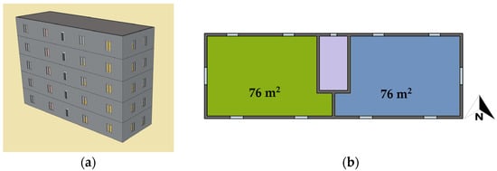
Figure 1.
The three-dimensional model (a) and plan of the building floors (b).
The building uses a central heating system with a conventional boiler, and heat is distributed via traditional radiators. To assess the impact of insulation measures and, more importantly, the impact of climate change on cooling demand, the use of air-conditioning units in each apartment was also considered. The heating system is in operation from 15 October to 15 April, maintaining a temperature of 20 °C for 14 h a day according to national regulations. In the cooling season, the air conditioner is turned on from 11:00 to 18:00 and from 20:00 to 22:00, maintaining the internal temperature at 28 degrees Celsius. The building and the system were modeled with DesignBuilder software ver. 7, and the calculations were performed using EnergyPlus ver. 9.04.
3.2. Renovation Process
The original building features poor thermal characteristics; therefore, in this study, four different refurbishment solutions were considered, and each of them includes the installation of a 12 cm layer of external thermal insulation EPS with added graphite (EPSG) with a thermal conductivity of λ = 0.032 W/(m K) (solutions 1 and 2), along with a 12 cm layer of EPS with a thermal conductivity of λ = 0.036 W/(m K) (solutions 3 and 4). Additionally, the roof was insulated with a 14 cm layer of material similar to that used for the walls in each solution, existing windows were replaced with low-emissivity triple glazing, and there was a possibility of installing an air-conditioning system (solutions 2 and 4). The building construction is massive, and the use of external insulation preserves the overall capacity of the building, possibly limiting the temperatures during the summer period or the energy required for air-conditioning. Table 1 shows the structural specifications of the building in both the original and renovated versions, with the addition of insulation layers to the walls and the replacement of windows. The insulation includes two typical materials used in external insulation; they slightly differ in thermal characteristics and in unit price.

Table 1.
The characteristics of the building’s opaque and transparent structures in the original and renovated conditions, with insulation layers made of EPS (expanded polystyrene) and EPS with graphite (EPSG).
3.3. Climate Files
Climate data are essential for conducting dynamic energy simulations in buildings, with Typical Reference Years (TRYs) commonly utilized for this purpose. According to UNI EN ISO 15927-4 [48], a reference year is an artificial year suitable for determining the average annual energy for heating and cooling [49]. The Typical Reference Year (TRY) represents the past and present climate conditions in which the building was constructed, operated, and continues to function. However, these conditions may differ significantly from the future climate in which the building will operate. Therefore, it is of utmost importance to consider climate change and rising temperatures in building energy simulations. In this work, the economic analysis was developed considering both the TRY file as the representative year of the 1995–2021 period and climate file projections for the FMY (Future Meteorological Year) obtained by the application of the EN ISO 15927-4 into the projected models. These models are available in the EURO-CORDEX (Coordinated Regional Climate Downscaling Experiment) dataset online [50], which were selected for a specific location using their coordinates (the longitude, latitude, and altitude of the desired weather station in Trieste), and FMYs were generated using two hourly climate models, namely GERICS_CNRM-CM5 and GERICS_IPSL-CM5A-MR, with the RCP 8.5 scenario already being used in the literature for deriving future weather scenarios [51,52], and for two different periods, 2020–2035 and 2036–2050, resulting in four future files. The models were selected because they provide hourly data. Morphing techniques were not used to generate future weather files. Furthermore, the use of two models allowed us to take into consideration the uncertainty in future weather projections. Weather files were generated using EN ISO 159827-4; therefore, they represent the mean behavior of the weather conditions suitable for computing energy consumption during the timeframe for which the TRY was generated. Each month of the TRY was selected from months pertaining to different years, and they also incorporate extreme events, such as heat waves, of the selected month. In this paper, the heatwave was considered as an event where the minimum and maximum daily temperature exceed 22 °C and 30 °C [53]. Each weather file was characterized by the total length of the heat wave, defined as the number of days which are part of such events. Table 2 presents the key attributes of the climate files used for the simulations, reporting the heating degree days (HDDs) and cooling degree days (CDDs) for a base temperature equal to 20 °C, the value of the average temperature during the heating period (θh, 1st of October–31st of March) and cooling period (θc, 1st of April–30th of September), and the heat wave’s total length (HW). In order to clearly identify each model and time interval in the following sections, the current climate file is indicated as PC_0, while for the projected data, the acronym FC is used, so the first model (GERICS_CNRM-CM5) and the first period are indicated by the 1_1, and the second period is denoted as 1_2, while the second model (GERICS_IPSL-CM5A-MR) is indicated with the numbers 2_1 and 2_2. The data presented in Table 2 show that, because of climate change, the heating degree days (HDDs) decrease, while the cooling degree days (CDDs) increase. Only a slight decrease in the mean temperature for FC_1_1 is presented, but still with an increase in HDD.
Table 2.
The number of HDDs and CDDs, the average temperature during the heating and cooling periods, and heat wave’s total length in each weather file.
3.4. Economic Calculation
The economic return of a renovation project can be assessed by calculating the Net Present Value (NPV), which incorporates both costs and savings accrued over a period of n years. This calculation uses an appropriate discount rate r, which must be adjusted to exclude the effects of inflation ri, resulting in the real discount rate rr.
The energy savings in natural gas consumption and electricity achieved through the requalification process translates into annual cash flow, which can be determined as
In this context, QSdF,i denotes the annual energy consumption of the original building, while Qriq,i represents the energy consumption of the retrofitted building, cgas is the energy cost for natural gas, and cele is the energy cost of electricity. The terms Sig and Sie take into account annual variations, especially when considering the impact of climate change. To optimize computational efficiency, the Si value was evaluated for two distinct periods: Sa for the 2022–2035 period and Sb for the 2036–2050 period. Assuming constant cash flows in each period and incorporating a rate of change in energy cost for natural gas re, the Net Present Value (NPV) can be calculated as follows:
The calculation, performed over a total duration of n years, was divided into two distinct periods: the first one is from year 1 to m, and the second one is from m+1 to n. This segmentation allows for a more precise representation of the variable conditions over the time span. Consequently, Equation (4) can be reformulated to derive the corresponding calculation expressed in Equation (5).
In Equation (5), the first two terms represent the cumulative sum of discounted cash flows for the period from year 1 to m, as outlined by Di Giuseppe et al. [29]. The third and fourth terms, namely Sbg and Sbe, capture the contribution of cash flow generated during the subsequent period from m + 1 to n, which is discounted to year m. The last term considers the cash flow obtained by the presence of an incentive of a yearly amount for a period of ninc years. This division ensures that temporal variations in cash flows are appropriately accounted for in the NPV calculation.
3.5. Estimation of Intervention Costs
The refurbishing intervention requires an initial investment which represents the initial cost C0. To compute such a term, all implementation phases of the intervention were considered:
- External thermal insulation and roof insulation with EPS or EPSG: Both interventions involve the initial removal of existing plaster and coatings, followed by the application of a rough cement coating to improve adhesion to the wall. This is followed by the installation of EPSG insulating panels (solutions 1 and 2) or EPS (solutions 3 and 4) and the creation of a finishing layer based on granular silicate.
- Window replacement: This intervention involves the removal of existing wooden frame windows and the subsequent installation of PVC frames with low-emissivity triple glazing with Argon and aluminum shutters.
- Installation of air-conditioning: This intervention involves the installation of an independent split-type air-conditioning system with a nominal thermal power of 3.8 kW (solutions 2 and 4). This case is related to possible high internal temperatures during the summer period, and it is considered as a future possibility for social housing and to deal with the increase in extreme events such as heat waves, as presented in Table 2, where the increase in the heat wave’s total length for future weather conditions is clearly shown.
This approach provides an evaluation of the actual cost of the interventions carried out on original buildings. The unit price for each execution phase was obtained from the Regional Price List of Public Works 2024 of the Autonomous Region of Friuli Venezia Giulia [54], where the building is located. In Table 3, all of the costs associated with the interventions are reported, and Table 4 reports the total cost of the renovation for each scenario, which was calculated for the whole building.
Table 3.
The cost of implementing individual phases of the intervention.
Table 4.
The cost of the analyzed intervention solutions.
3.6. Uncertainty Analysis
In energy and economic analysis in buildings, a simplifying assumption is to deal with constant parameters; however, some parameters, starting from economic ones, can be affected by uncertainties. In this study, the polynomial chaos expansion method was implemented to deal with two economic parameters described with a statistical distribution. Therefore, system economic performance can only be described through a cumulative distribution function, and the results will be given as a success probability or as a percentile distribution, as outlined by Manzan et al. [55].
3.7. Economic Data
An economic performance assessment of the proposed renovation solutions was performed using the parameter values listed in Table 3 and Table 4. These parameters were assumed to be constant over time, as reported in Table 5, except for the natural gas energy price, which was modeled using logistic distribution. In addition, a stochastic process was considered for the initial investment cost, PC0. While this parameter is typically fixed and known in conventional design practices, real-world scenarios often involve variations between the design and construction phases, as evidenced by the recent significant increase in construction material costs [29]. To account for this, a uniform probability distribution was applied, with the uniform distribution ranging from −8% to +8% of the computed cost. The integration of random inputs leads to outputs characterized by statistical distributions. As a result, the analysis provides a confidence value associated with the Net Present Value (NPV). Two approaches were considered, with the former being more conservative, namely defining the tenth percentile (NPV10) as the value to be obtained with more than a 90% probability of being achieved, and the latter being more relaxed, namely defining the fiftieth percentile (NPV50) with a 50% probability of being achieved.
3.8. Introduction to Polynomial Chaos Expansion
The problem is not deterministic since two parameters are described by statistical distributions, namely the initial cost C0 and the increment in energy cost re. The classical way to deal with such problems is the Montecarlo method. However, this method is characterized by slow convergence, requiring the generation of a large number of samples and requiring an intensive computational load if the function to be evaluated is complex. A different way to address the problem is to use the polynomial chaos expansion (PCE). This expansion is described by Equation (6):
is a function that depends on deterministic variables x and stochastic variables as described by statistical distributions; in the present case, the function corresponds to Equation (5), while M is the polynomial order. The function is approximated by the combination of polynomials as a function of the stochastic variables and spectral coefficients . To generate the expansion, in this paper, we used the Python (version 3.12.0) library chaospy [56,57], which provides different methods to create the expansion described in Equation (6). In this paper, the pseudo-spectral method was implemented, adopting a Gaussian quadrature with 25 points and polynomials of order M = 3. The main feature of the polynomial chaos method is that only 25 evaluations on quadrature points are required; on the contrary, the Montecarlo method requires thousands of evaluations. Once the surrogate model is obtained, it can be used to derive statistical moments and the desired percentiles by Montecarlo sampling but with a faster rate, since the evaluation of the surrogate model is faster than the original model. Appendix A reports the steps taken to obtain the required percentiles.
Table 5.
Economic parameters. (* It is the reference for computing Inflation rate).
Table 5.
Economic parameters. (* It is the reference for computing Inflation rate).
| Parameter | Value | Unit | Source |
|---|---|---|---|
| Gas | 0.978 | €/st m3 | ARERA [58] |
| Electricity | 0.23455 | €/kWh | ARERA |
| Inflation rate * (ri) | 1.678 | % | Worldwide Inflation Data: www.inflation.eu (accessed on 10 March 2025) |
| Discount rate (r) | 2.75 | % | Bank of Italy |
| Energy price trend (re) | Loc 3.3738 Scale 1.5797 | % | ARERA |
* mean 2013–2024.
3.9. Choice of Funding Scenarios
As mentioned in the introduction, for the purposes of the present analysis, two tax deduction alternatives were considered and applied to the interventions analyzed. The first alternative (best-case scenario) assumes access to the Superbonus and a 65% tax deduction; the second (worst-case scenario) only considers access to the Ecobonus, with a 36% tax deduction (assuming a plausible scenario in which expenses for interventions on the first home are incurred by 2026).
4. Results
The EnergyPlus simulation software was used to run simulations for both models in the current state of the building and its condition after retrofitting. Climate baseline years, created for both current and future scenarios, were formatted into EPW files to serve as climate input data for hourly energy simulations conducted in EnergyPlus. The annual energy consumption for heating and the electricity demand for air-conditioning were calculated for each configuration. However, these data should be considered as indicative as they assume general cooling in all areas; in the results, this metric will only be used to compare the various configurations since in social housing, the installation of cooling systems is usually performed by the apartment owner or tenant alone.
Table 6 provides a detailed summary of the simulation results, referring to the initial setup results for the various climate scenarios described in Table 2. The results indicate a clear pattern: as the analysis moves from current climate conditions to future scenarios, there is a significant decrease in gas consumption for heating, which is associated with an increase in electricity consumption for air-conditioning. This change reflects the projected impacts of climate change on energy demand patterns. Furthermore, energy retrofitting proves highly effective in reducing heating energy consumption. Although cooling energy consumption also decreases, the reduction is less pronounced than that of heating energy consumption. This discrepancy can be attributed to the significant difference between the number of heating degree days and cooling degree days, as documented in Table 2. The results highlight the critical role of climate factors in shaping energy performance, especially in regions with significant seasonal variations. Figure 2a compares the natural gas energy of the different solutions with the significant decrease in heating energy required with the renovation of the building, with slightly lower performance for the solution using EPS and graphite. Figure 2b compares the electrical energy required; in this case, the differences are less identifiable, with an increase in electrical energy for the renovated building and current weather file, the PC_0 case, and a reduction for future cases (FCs) in the renovated building. Figure 2 shows the increase in energy required for cooling and reduction in heating with future weather data.
Table 6.
The relative results of the simulations with respect to the non-insulated building and current PC_0 climate data, the gas consumption, and the electricity consumption due to the use of air conditioners.

Figure 2.
Comparison of energy between different cases. (a) Natural gas energy. (b) Electricity.
Economic Results
Table 7 reports the results of economic calculations in terms of NPV and the difference in NPV with the two incentives, providing insights into the potential long-term economic effects of the proposed interventions. The calculations were executed considering a total period of n = 30 years and a first period of m = 14 years, first excluding stochastic variations in input parameters to simplify the analysis. The first evaluation period runs from 2022 to 2035, capturing short- and medium-term impacts, while the second period extends from 2026 to 2051, allowing for a comprehensive assessment of the interventions’ performance over a longer time frame. As premised in Section 2, two levels of incentives were considered, namely 36% and 65% of the initial investment cost, spread over a 10-year period. The results in Table 7 show that, in the worst-case scenario (36% tax deduction), the NPV is always negative, indicating that no intervention is profitable. However, if a 65% tax deduction is considered, the NPV for solution 1 with the current climate file (PC_0) and that for solution 3 with both the current climate file and future climate file 1 (FC_1) are positive. In both tax deduction scenarios, solutions 2 and 4, which involve the installation of an air-conditioning system, have negative NPVs. However, the NPV delta between the two tax deduction scenarios is always significant: it is nearly EUR 83.000 on average, which, depending on the solution, represents a percentage between 25% and 30% of the initial investment cost.
Table 7.
Net Present Value under different conditions and two incentives.
Furthermore, the use of future weather data always reduces the NPV, confirming the need to consider future weather trends when planning a building renovation.
The introduction of uncertainty affects the calculated NPVs because they become statistical distributions rather than determined results. The NPV is expressed in terms of percentiles by introducing NPV10 and NPV50. It is important to note that the deterministic NPV obtained using Equation (3), with the deterministic parameters, is not directly comparable to any of the NPV10 and NPV50 values. Table 8 presents the NPV corresponding at the 10th percentile for both incentives.
Table 8.
Solutions with uncertainty; NPV 10th percentile.
Table 9 presents the same results using the 50th percentile. As expected, NPV50 is greater than NPV10 since a lower success probability is considered. Specifically, in the case of the NPV at the 10th percentile (Table 8), even with a 65% tax deduction, all NPVs remain negative; however, the average NPV delta, as well as its percentage of the initial investment cost, remains in line with the case without uncertainty (Table 7). The same applies to the NPV at the 50th percentile (Table 9): in this case, as in the scenario without uncertainty, the NPVs for solution 1 and solution 3 with the current climate file are positive, while those for solutions 2 and 4 remain negative.
Table 9.
Solutions with uncertainty; NPV 50th percentile.
The inspection of the results also shows the negative impact of climate change on the NPV, NPV10 and NPV50 with a reduction in respective values in both the deterministic and probabilistic scenarios.
The results of the analysis highlight four significant aspects:
- For investments to be economically viable, it is necessary to have substantial incentive measures, which, if solely represented by tax deductions, may still prove insufficient. This result reinforces the CNI’s calls for the development of a robust financial plan to support the upcoming national building renovation plan aimed at achieving the objectives of the EPBD.
- Considering the effects of climate change (increased average external temperature, more frequent heatwaves, etc.) on indoor comfort conditions in buildings and human well-being, the installation of air-conditioning systems is becoming an increasingly common and established solution. While this type of solution may not be ideal for human health, especially for vulnerable groups, the lack of profitability of such interventions even with significant tax deductions (e.g., 65%) is, at present, an aspect that needs to be taken into account. This result further reinforces the CNI’s observations on the need for an adequate financial plan to support energy renovation interventions and simultaneously urges prioritizing the investigation of alternative solutions for summer air-conditioning to protect both human health and the environment.
- While interventions such as external insulation and window replacement improve the winter performance of buildings by reducing energy consumption, they may exacerbate the internal environmental conditions of buildings during the summer season. This could further encourage individuals to resort to traditional air-conditioning systems (such as split units), for which the observations in the previous point are even more valid.
- There is a small difference between the EPSG and EPS results and the results obtained with EPS, with a slightly higher NPV for all cases; this means that the higher cost of EPSG is not compensated for by the slightly better thermal characteristics of the material.
In conclusion, to understand the feasibility and cost-effectiveness of interventions, evaluating their economic viability is just as important as the results they can yield from an energy perspective. This is particularly true for buildings like the one analyzed in this work, where the possibility of carrying out interventions must necessarily be weighed against the financial resources of the tenants, which are often limited.
5. Discussion and Conclusions
This study investigates the renovation of a building, originally characterized by poor thermal constructions typical of a social housing building in Trieste. The proposed interventions include the installation of external insulation on the walls and roofs and the replacement of existing windows to improve energy efficiency. The performance of these retrofit measures was assessed through detailed simulations carried out in EnergyPlus, using several climate files to analyze the potential impact of climate change on energy demand. The climate data included a historical file representing conditions in Trieste for the 1995–2021 period and future climate projections for the 2020–2035 and 2036–2050 periods, generated using GCM-RCM climate models. The analysis provided insights into energy consumption for heating and cooling under different scenarios. The results confirm that with future temperature increases, heating demand decreases, while cooling demand increases, changing the energy balance required for the building. This trend highlights the increasing importance of designing interventions that not only address heating efficiency but also mitigate the increasing demand for cooling in hot climates.
In addition to an energy performance analysis, an economic evaluation of the interventions was conducted by calculating the Net Present Value (NPV) of the investment costs. The economic analysis included scenarios with incentives that provided paybacks of 65% and 36% of the initial investment over a ten-year period. The analysis showed that incentives play an important role in making retrofitting economically viable, especially when addressing the existing building stock, which often requires significant financial inputs for renovation. To address uncertainties in the initial investment and energy costs, a probabilistic approach was applied considering statistical distributions of the input parameters. One limitation of this approach is the number of parameters described by statistical distributions, and each parameter is stochastically independent from the others. Other economic parameters will be added in the future, such as interest rates and inflation, but this will require a multivariate analysis since different parameters could be statistically correlated. The NPV percentiles were calculated with a specific focus on the 10th percentile, which serves as a conservative benchmark for investors by providing a lower estimate of profitability; additionally, a more relaxed solution with the 50th percentile was studied. This approach highlights the variability and potential risks associated with economic returns and reinforced the need for robust incentive mechanisms to compensate for these uncertainties. The results also show the impact of climate change on economic parameters that are negatively affected by rising temperatures with a decrease in the NPV. When comparing the results shown in Table 7, it can be seen that the NPV for cases FC_1 and FC_2 is always lower than the one for FC_0; the maximum variation is seen for the insulation with EPSG and AC, with reductions of 3.21% and 6.96% with respect to investment costs for FC_1 and FC_2, respectively; and both levels of incentives have similar values for the other cases. The same results can be seen in Table 8 and Table 9 reporting NPV10 and NPV50. For NPV10, as shown in Table 8, the maximum effect of climate change is seen for the solution with EPSG and FC_2 with a maximum reduction of 4.59% with respect to the initial cost; for NPV50, as shown in Table 9, the maximum reduction achieved is 6.65% with FC_2 and EPSG without cooling. Considering the mean values of changes for each climate, FC_1 generates a mean change of 1.73% for NPV10 and 2.82% for NPV50, while with FC_2, the mean change values are 4.39% and 6.57% for NPV10 and NPV50, respectively.
These findings highlight the significant impact of rising temperatures on energy and economic outcomes. In particular, the reduction in heating demand due to milder winters results in lower profit margins for interventions that solely target heating efficiency. This reduction in economic viability highlights the need for a comprehensive approach to building retrofitting that addresses the dual challenges of reducing heating and cooling demand. Furthermore, this study highlights the critical importance of incentive programs to encourage the energy-efficient renovation of existing buildings. Without adequate financial support, the economic returns of such interventions may be insufficient to attract investors, especially in cases where climate conditions result in potential savings from reduced heat energy consumption.
This study relies on the availability of future weather projections. In this paper, the GERICS_CNRM-CM5 GERICS and _IPSL-CM5A-MR coupled GCM-RCM models were used. However, to enlarge the significance of the results, more models should be considered. In the present paper, only models available to the authors with hourly data were considered, so the addition of supplementary models could improve the results, giving rise to numerically different NPVs without jeopardizing the main results obtained since the future increase in temperature is a common feature of all the models. An additional limitation of this work comes from the method utilized to generate weather data for the simulations. The files describe a mean year incorporating only a part of extreme events that can temporarily increase energy consumption if cooling systems are considered. However, the choice is consistent with the scope of the current work that focuses on energy consumption and related economic analysis. A more detailed analysis of how extreme heat events could affect people’s comfort and energy consumption is needed.
In conclusion, this work demonstrates that building retrofitting can provide significant energy and economic benefits when designed with current and future climate conditions in mind. However, the findings also highlight the importance of integrating policy measures, such as financial incentives, to increase the feasibility and attractiveness of such interventions. As climate change continues to affect building energy dynamics, future studies should explore adaptive strategies that balance heating and cooling requirements and ensure that retrofitting measures remain effective and economically viable under different climate scenarios. An important outcome of the work is that the EPBD IV decarbonization of the Union’s stock requires strong incentive support and price control to make building refurbishment attractive for investors. The polynomial chaos method introduced in this paper represents a viable approach for introducing uncertainty analysis for problems that require high computational costs where classical Montecarlo systems could be too slow because of the high number of evaluations required. New or improved strategies should be implemented with a broader use of heat pumps, possibly accompanied by the exploitation of renewable energy sources, in particular photovoltaics systems. Technical solutions should also be accompanied by new policy approaches. As an example, energy sharing between users in energy communities could represent a viable answer for reducing climate change impact.
Author Contributions
Conceptualization, M.M. and A.R.; methodology, A.R.; software, A.R. and M.M.; validation, A.R.; formal analysis, M.M.; investigation, A.R.; resources, M.M.; data curation, A.R. and J.J.C.; writing—original draft preparation, A.R.; writing—review and editing, A.R., M.M. and J.J.C.; supervision, M.M.; funding acquisition, M.M. All authors have read and agreed to the published version of the manuscript.
Funding
The future weather files used in this paper were generated using the methodologies developed within the “Climate Resilient Strategies by Archetype-based Urban Energy Modelling (CRiStAll)” project funded by the European Union—Next Generation EU within the PRIN 2022 PNRR program (D.D. 1409 of 14/09/2022 Ministero dell’Università e della Ricerca), M4C2, I 1.1. This manuscript reflects only the authors’ views and opinions, and the Ministry cannot be considered responsible for them.
Data Availability Statement
No new data were created or analyzed in this study. Data sharing is not applicable to this article.
Acknowledgments
The authors wish to thank the support provided by the Azienda Territoriale per l’Edilizia Residenziale di Trieste, ATER.
Conflicts of Interest
The authors declare no conflicts of interest.
Appendix A
Chaospy is a python library that provides several utilities to deal with uncertain parameters. Here, the chaospy library was exploited to obtain the percentiles of the Net Present Value with two stochastic parameters described by distributions; the gas cost increment re uses a logistic distribution, while the initial cost C0 is represented by a uniform distribution around the computed cost. Table A1 describes the implemented procedure step by step. In steps 1 and 2, a multivariate joint distribution is created; this is the distribution from which the sample will be taken in the next steps. The Gaussian quadrature is obtained in step 3, with the generation of Gauss quadrature nodes and respective weights. In step 4, the NPV is calculated using a routine which implements Equation (5) using the coordinates of the Gauss nodes (re and C0) previously identified. Step 5 generates the polynomials to be used for the expansion; while in step 6 the model approximation is created using the polynomial expansion and generating the coefficients of Equation (1). Once the gauss_approx has been obtained in step 6 the approximation can be used to compute the percentiles in step 7. The last step is taken using the approximation; or surrogate model; with is faster than the original model. It is worth noting that the steps 1, 2, 4 and 7, with samples in 4 obtained using the joint distribution in 2, and in 7 using directly the evaluations in step 4 represent the Montecarlo approach.
Table A1.
Pseudocode for generating percentiles using polynomial chaos quadrature.
Table A1.
Pseudocode for generating percentiles using polynomial chaos quadrature.
| Steps | Chaospy Pseudocode | |
|---|---|---|
| 1 | Create distributions of stochastic variables | Re_dist = Logistic (skew = 1, 0.033738, 0.01579708) IC_dist = Uniform (IC * 0.92, IC * 1.08) |
| 2 | Create joint distribution | joint = J (Re_dist, IC_dist) |
| 3 | Create quadrature with nodes and weights | gauss_q, weights = generate_quadrature (order = 4, joint, rule = “gauss”) |
| 4 | Compute function at quadrature points using Equation (5) | evals = calcVAN (gauss_q) |
| 5 | Define polynomials (order 3) | expansion = generate_expansion (order = 3, joint) |
| 6 | Generate model approximation | approx = fit_quadrature (expansion, gauss_q, weights, evals) |
| 7 | Compute 10th and 50th percentiles with model approximation and N samples | perc10 = Perc (approx, 10, joint, N) perc50 = Perc (approx, 50, joint, N) |
References
- Yang, Y.; Javanroodi, K.; Nik, V.M. Climate Change and Energy Performance of European Residential Building Stocks—A Comprehensive Impact Assessment Using Climate Big Data from the Coordinated Regional Climate Downscaling Experiment. Appl. Energy 2021, 298, 117246. [Google Scholar] [CrossRef]
- Li, Y.; Wang, W.; Wang, Y.; Xin, Y.; He, T.; Zhao, G. A Review of Studies Involving the Effects of Climate Change on the Energy Consumption for Building Heating and Cooling. Int. J. Environ. Res. Public Health 2020, 18, 40. [Google Scholar] [CrossRef] [PubMed]
- Barbosa, R.; Vicente, R.; Santos, R. Climate Change and Thermal Comfort in Southern Europe Housing: A Case Study from Lisbon. Build. Environ. 2015, 92, 440–451. [Google Scholar] [CrossRef]
- Calvin, K.; Dasgupta, D.; Krinner, G.; Mukherji, A.; Thorne, P.W.; Trisos, C.; Romero, J.; Aldunce, P.; Barrett, K.; Blanco, G.; et al. Climate Change 2023: Synthesis Report. Contribution of Working Groups I, II and III to the Sixth Assessment Report of the Intergovernmental Panel on Climate Change; Core Writing Team, Lee, H., Romero, J., Eds.; First Intergovernmental Panel on Climate Change (IPCC), 25 July 2023; IPCC: Geneva, Switzerland, 2023. [Google Scholar] [CrossRef]
- Elnagar, E.; Gendebien, S.; Georges, E.; Berardi, U.; Doutreloup, S.; Lemort, V. Framework to Assess Climate Change Impact on Heating and Cooling Energy Demands in Building Stock: A Case Study of Belgium in 2050 and 2100. Energy Build. 2023, 298, 113547. [Google Scholar] [CrossRef]
- Tahir, F.; Al-Ghamdi, S.G. Climatic Change Impacts on the Energy Requirements for the Built Environment Sector. Energy Rep. 2022, 9, 670–676. [Google Scholar] [CrossRef]
- Hernandez-Cruz, P.; Giraldo-Soto, C.; Escudero-Revilla, C.; Hidalgo-Betanzos, J.M.; Flores-Abascal, I. Energy Efficiency and Energy Performance Gap in Centralized Social Housing Buildings of the Basque Country. Energy Build. 2023, 298, 113534. [Google Scholar] [CrossRef]
- Tootkaboni, M.P.; Ballarini, I.; Corrado, V. Analysing the Future Energy Performance of Residential Buildings in the Most Populated Italian Climatic Zone: A Study of Climate Change Impacts. Energy Rep. 2021, 7, 8548–8560. [Google Scholar] [CrossRef]
- Wehrli, K.; Sidler, F.; Gubler, S.; Settembrini, G.; Koschenz, M.; Irigoyen, S.D.; Kotlarski, S.; Fischer, A.M.; Zweifel, G. Building Design in a Changing Climate—Future Swiss Reference Years for Building Simulations. Clim. Serv. 2024, 34, 100448. [Google Scholar] [CrossRef]
- Bazazzadeh, H.; Nadolny, A.; Safaei, S.S.H. Climate Change and Building Energy Consumption: A Review of the Impact of Weather Parameters Influenced by Climate Change on Household Heating and Cooling Demands of Buildings. Eur. J. Sustain. Dev. 2021, 10, 1–12. [Google Scholar] [CrossRef]
- Salata, F.; Falasca, S.; Ciancio, V.; Curci, G.; de Wilde, P. Climate-Change Related Evolution of Future Building Cooling Energy Demand in a Mediterranean Country. Energy Build. 2023, 290, 113112. [Google Scholar] [CrossRef]
- Dodoo, A.; Gustavsson, L. Energy Use and Overheating Risk of Swedish Multi-Storey Residential Buildings under Different Climate Scenarios. Energy 2016, 97, 534–548. [Google Scholar] [CrossRef]
- Hernandez-Cruz, P.; Flores-Abascal, I.; Hidalgo-Betanzos, J.M.; Almeida, M.; Erkoreka-Gonzalez, A. Environmental and Energy Analysis of the Renovation of Social Housing Buildings under Various Climate Change Scenarios and User Profiles. J. Build. Eng. 2024, 98, 111164. [Google Scholar] [CrossRef]
- Huang, K.-T.; Hwang, R.-L. Future Trends of Residential Building Cooling Energy and Passive Adaptation Measures to Counteract Climate Change: The Case of Taiwan. Appl. Energy 2016, 184, 1230–1240. [Google Scholar] [CrossRef]
- Mancini, F.; Basso, G.L. How Climate Change Affects the Building Energy Consumptions Due to Cooling, Heating, and Electricity Demands of Italian Residential Sector. Energies 2020, 13, 410. [Google Scholar] [CrossRef]
- Jalali, Z.; Shamseldin, A.Y.; Ghaffarianhoseini, A. Impact Assessment of Climate Change on Energy Performance and Thermal Load of Residential Buildings in New Zealand. Build. Environ. 2023, 243, 110627. [Google Scholar] [CrossRef]
- Nik, V.M.; Kalagasidis, A.S. Impact Study of the Climate Change on the Energy Performance of the Building Stock in Stockholm Considering Four Climate Uncertainties. Build. Environ. 2013, 60, 291–304. [Google Scholar] [CrossRef]
- Campagna, L.M.; Fiorito, F. On the Impact of Climate Change on Building Energy Consumptions: A Meta-Analysis. Energies 2022, 15, 354. [Google Scholar] [CrossRef]
- Liu, S.; Wang, Y.; Liu, X.; Yang, L.; Zhang, Y.; He, J. How Does future climatic uncertainty affect multi-objective building energy retrofit decisions? Evidence from residential buildings in subtropical Hong Kong. Sustain. Cities Soc. 2023, 92, 104482. [Google Scholar] [CrossRef]
- Corrado, V.; Ballarini, I. Refurbishment Trends of the Residential Building Stock: Analysis of a Regional Pilot Case in Italy. Energy Build. 2016, 132, 91–106. [Google Scholar] [CrossRef]
- Ascione, F.; Cheche, N.; De Masi, R.F.; Minichiello, F.; Vanoli, G.P. Design the Refurbishment of Historic Buildings with the Cost-Optimal Methodology: The Case Study of a XV Century Italian Building. Energy Build. 2015, 99, 162–176. [Google Scholar] [CrossRef]
- Manzan, M.; Ramezani, A. Analisi dell’incertezza economica nella riqualificazione energetica degli edifici nel contesto del cambiamento climatico (Analysis of the economic uncertainty in the energy requalification of buildings in a climate change context). In Proceedings of the 39th AiCARR National Conference, Napoli, Italy, 8 September 2023. [Google Scholar]
- Chari, A.; Xanthos, S.; Christodoulou, S.E. Stochastic Assessment of the Energy Performance of Buildings. Energy Effic. 2017, 10, 1573–1591. [Google Scholar] [CrossRef]
- Mata, É.; Wanemark, J.; Nik, V.M.; Kalagasidis, A.S. Economic Feasibility of Building Retrofitting Mitigation Potentials: Climate Change Uncertainties for Swedish Cities. Appl. Energy 2019, 242, 1022–1035. [Google Scholar] [CrossRef]
- Pezzi, A.; Manzan, M.; Rosato, P. The Impact of Climate Change on the Reliable Optimization for Energy and Economic Refurbishment of a Residential Building in Italy. In Proceedings of the Building Simulation 2021: 17th Conference of IBPSA, Bruges, Belgium, 1–3 September 2021; pp. 861–869. [Google Scholar] [CrossRef]
- Mostafazadeh, F.; Eirdmousa, S.J.; Tavakolan, M. Energy, Economic and Comfort Optimization of Building Retrofits Considering Climate Change: A Simulation-Based NSGA-III Approach. Energy Build. 2022, 280, 112721. [Google Scholar] [CrossRef]
- Sun, S.; Kensek, K.; Noble, D.; Schiler, M. A Method of Probabilistic Risk Assessment for Energy Performance and Cost Using Building Energy Simulation. Energy Build. 2016, 110, 1–12. [Google Scholar] [CrossRef]
- Prada, A.; Pernigotto, G.; Baggio, P.; Gasparella, A. Uncertainty Propagation of Material Properties in Energy Simulation of Existing Residential Buildings: The Role of Buildings Features. Build. Simul. 2017, 11, 449–464. [Google Scholar] [CrossRef]
- Di Giuseppe, E.; Massi, A.; D’orazio, M. Probabilistic Life Cycle Cost Analysis of Building Energy Efficiency Measures: Selection and Characterization of the Stochastic Inputs through a Case Study. Procedia Eng. 2017, 180, 491–501. [Google Scholar] [CrossRef]
- Esther, D.; Banyk, A.; Smith, J.; Adelusi, J.B. The Future of AI in Climate-Focused Financial Modeling and Impact Assessment Govik Twenty Five. February 2025. Available online: https://www.researchgate.net/publication/388688332 (accessed on 24 March 2025).
- Akram, B.; Abbas, A. AI and Machine Learning in Financial Forecasting: Driving Sustainable Finance and Energy Policy. February 2025. [Google Scholar] [CrossRef]
- Bahmani, M.H.; Shayan, M.E.; Fioriti, D. Assessing electric vehicles behavior in power networks: A non-stationary discrete Markov chain approach. Electr. Power Syst. Res. 2024, 229, 110106. [Google Scholar] [CrossRef]
- Dotzler, C.; Botzler, S.; Kierdorf, D.; Lang, W. Methods for optimising energy efficiency and renovation processes of complex public properties. Energy Build. 2018, 164, 254–265. [Google Scholar] [CrossRef]
- Martini, S.; Morgut, M.; Pigazzini, R.; Parussini, L. Uncertainty quantification and sensitivity analysis of the SST turbulence model applied to VIV. J. Fluids Struct. 2024, 133, 104225. [Google Scholar] [CrossRef]
- Korondi, P.Z.; Marchi, M.; Parussini, L.; Quagliarella, D.; Poloni, C. Multi-Objective Design Optimisation of an Airfoil with Geometrical Uncertainties Leveraging Multi-Fidelity Gaussian Process Regression. In Advances in Uncertainty Quantification and Optimization Under Uncertainty with Aerospace Applications. UQOP 2020; Space Technology Proceedings; Vasile, M., Quagliarella, D., Eds.; Springer: Cham, Switzerland, 2020; Volume 8. [Google Scholar] [CrossRef]
- European Commission. Directive (EU) 2024/1275 of the European Parliament and of the Council of 24 April 2024 on the Energy Performance of Buildings. 2024. Available online: https://eur-lex.europa.eu/eli/dir/2024/1275/oj/eng (accessed on 21 March 2025).
- Ministero dell’Ambiente e della Sicurezza Energetica. La Situazione Energetica Nazionale nel 2023. 2024; p. 61. Available online: https://www.mase.gov.it/sites/default/files/Archivio_Energia/LA%20RELAZIONE%20SULLA%20SITUAZIONE%20ENERGETICA%20NAZIONALE%20NEL%202022_MASE%20Luglio%202023.pdf (accessed on 13 February 2025).
- ISPRA. Le Emissioni di Gas Serra in Italia. Obiettivi di Riduzione al 2030. 2024; p. 40. Available online: https://www.isprambiente.gov.it/files2024/pubblicazioni/rapporti/rapporto-399-24-le-emissioni-di-gas-serra-in-italia.pdf (accessed on 3 March 2025).
- European Commission. A Renovation Wave for Europe—Greening Our Buildings, Creating Jobs, Improving Lives. 2020. Available online: https://eur-lex.europa.eu/legal-content/EN/TXT/?uri=CELEX:52020SC0550 (accessed on 21 March 2025).
- European Commission. The European Green Deal. 2019. Available online: https://eur-lex.europa.eu/legal-content/EN/TXT/?uri=celex%3A52019DC0640 (accessed on 21 March 2025).
- Consiglio Nazionale degli Ingegneri. Centro Studi CNI: Essenziale Attivarsi Subito per Definire il Piano Nazionale di Ristrutturazione per le Case Green. 2024. Available online: https://biblus.acca.it/piano-nazionale-di-ristrutturazione-case-green/ (accessed on 21 March 2025).
- Decreto Legge 19 Maggio 2020, n. 34. Misure Urgenti in Materia di Salute, Sostegno al Lavoro e All’economia, Nonché di Politiche Sociali Connesse All’emergenza Epidemiologica da COVID-19. Available online: https://www.gazzettaufficiale.it/atto/vedimenuhtml?atto.datapubblicazionegazzetta=2020-05-19&atto.codiceredazionale=20g00052&tiposerie=serie_generale&tipovigenza=originario (accessed on 21 March 2025).
- Legge 30 Dicembre 2024, n. 207. Bilancio di Previsione dello Stato per L’anno Finanziario 2025 e Bilancio Pluriennale per il Triennio 2025–2027. Available online: https://www.gazzettaufficiale.it/eli/id/2024/12/31/24G00229/SG (accessed on 21 March 2025).
- Decreto Legge 4 Giugno 2013, n. 63. Disposizioni Urgenti per il Recepimento della Direttiva 2010/31/UE del Parlamento europeo e del Consiglio del 19 Maggio 2010, Sulla Prestazione Energetica Nell’edilizia per la Definizione delle Procedure d’infrazione Avviate dalla Commissione Europea, Nonché Altre Disposizioni in Materia di Coesione Sociale. Available online: https://www.gazzettaufficiale.it/eli/id/2013/06/05/13G00107/sg (accessed on 21 March 2025).
- TABULA WebTool. 2014. Available online: https://webtool.building-typology.eu/#bm (accessed on 5 February 2025).
- Lupato, G.; Manzan, M. Italian TRYs: New weather data impact on building energy simulations. Energy Build. 2019, 185, 287–303. [Google Scholar] [CrossRef]
- EN 16798-1:2019; Energy Performance of Buildings—Part 1: Indoor Environmental Input Parameters for Design and Assessment of Energy Performance of Buildings Addressing Indoor Air Quality, Thermal Environment, Lighting and Acoustics—Module M1-6. Committee for European Standardisation (CEN): Brussels, Belgium, 2019.
- EN ISO 15927-4:2005; Hygrothermal Performance of Buildings—Calculation and Presentation of Climatic Data—Part 4: Hourly Data for Assessing the Annual Energy Use for Heating and Cooling. Committee for European Standardisation (CEN): Brussels, Belgium, 2005.
- Skeiker, K. Comparison of methodologies for TMY generation using 10 years data for Damascus, Syria. Energy Convers. Manag. 2007, 48, 2090–2102. [Google Scholar] [CrossRef]
- Available online: https://cordex.org/ (accessed on 21 March 2025).
- Bartók, B.; Tobin, I.; Vautard, R.; Vrac, M.; Jin, X.; Levavasseur, G.; Denvil, S.; Dubus, L.; Parey, S.; Michelangeli, P.-A.; et al. A climate projection dataset tailored for the European energy sector. Clim. Serv. 2019, 16, 100138. [Google Scholar] [CrossRef]
- Coppola, E.; Nogherotto, R.; Ciarlo’, J.M.; Giorgi, F.; van Meijgaard, E.; Kadygrov, N.; Iles, C.; Corre, L.; Sandstad, M.; Somot, S.; et al. Assessment of the European Climate Projections as Simulated by the Large EURO-CORDEX Regional and Global Climate Model Ensemble. J. Geophys. Res. Atmos. 2021, 126, e2019JD032356. [Google Scholar] [CrossRef]
- Casati, B.; Yagouti, A.; Chaumont, D. Regional Climate Projections of Extreme Heat Events in Nine Pilot Canadian Communities for Public Health Planning. J. Appl. Meteorol. Clim. 2013, 52, 2669–2698. [Google Scholar] [CrossRef]
- Regione Autonoma Friuli Venezia Giulia. Prezzario Regionale dei Lavori Pubblici. 2024. Available online: https://www.regione.fvg.it/rafvg/cms/RAFVG/infrastrutture-lavori-pubblici/lavori-pubblici/prezzario-2024/ (accessed on 3 March 2025).
- ARERA—Autorità di Regolazione per Energia Reti e Ambiente. Andamento del Prezzo del Gas Naturale per un Consumatore Domestico Tipo in Regime di tutela (Natural Gas Price Trend for a Domestic Consumer in the Protected Regime). 2023. Available online: https://www.arera.it/it/dati/gp27new.htm (accessed on 26 December 2024).
- Manzan, M.; Lupato, G.; Pezzi, A.; Rosato, P.; Clarich, A. Reliability-Based Optimization for Energy Refurbishment of a Social Housing Building. Energies 2020, 13, 2310. [Google Scholar] [CrossRef]
- Feinberg, J.; Langtangen, H.P. Chaospy: An open source tool for designing methods of uncertainty quantification. J. Comput. Sci. 2015, 11, 46–57. [Google Scholar] [CrossRef]
- Feinberg, J.; Eck, V.G.; Langtangen, H.P. Multivariate polynomial chaos expansions with dependent variables. SIAM J. Sci. Comput. 2018, 40, 199–223. [Google Scholar] [CrossRef]
Disclaimer/Publisher’s Note: The statements, opinions and data contained in all publications are solely those of the individual author(s) and contributor(s) and not of MDPI and/or the editor(s). MDPI and/or the editor(s) disclaim responsibility for any injury to people or property resulting from any ideas, methods, instructions or products referred to in the content. |
© 2025 by the authors. Licensee MDPI, Basel, Switzerland. This article is an open access article distributed under the terms and conditions of the Creative Commons Attribution (CC BY) license (https://creativecommons.org/licenses/by/4.0/).