Enhanced Fault Localization for Active Distribution Networks via Robust Three-Phase State Estimation

Abstract

Accurate fault localization is critical for ensuring reliable power supply in active distribution networks, yet conventional state estimation (SE)-based methods fail to differentiate authentic fault responses from measurement distortions due to uncertainties in fault parameters. To overcome this limitation, a robust three-phase SE-driven fault localization methodology is proposed. First, a measurement transformation-based SE model is built for fault conditions, leveraging real-time voltage phasor measurements and pseudo-measurements derived from pre-fault SE results. Then, a robust fault SE model is built using the quadratic-constant-based generalized maximum likelihood estimation, solved through the iteratively reweighted least squares algorithm that postpones phasor measurement weight updates until after initial iterations to prevent residual contamination. Furthermore, a fault localization algorithm is proposed through the systematic traversal of candidate buses, where each potential fault localization is assessed by performing robust fault SE with the fault current injected into this bus. The matching index is designed, accounting for the weight disparity of different types of measurements and measurement placement. Extensive simulations on a 33-bus unbalanced distribution network validate the method’s effectiveness under various measurement noise levels, fault resistances and incorrect data severity. The approach maintains comparable accuracy to conventional SE under normal operating conditions, while it exhibits superior robustness against measurement anomalies and effectively preserves fault localization reliability when confronted with incorrect data.

1. Introduction

As the final link in the electricity delivery chain, distribution networks constitute critical infrastructure for maintaining reliable power supply to end-users. However, distribution networks exhibit significantly higher fault probabilities compared to transmission systems due to their structural complexity and harsh operational environments. The faults occurring in distribution networks are predominantly short-circuit faults, including single-phase-to-ground, phase-to-phase, double-phase-to-ground, and three-phase short circuits. Among these, single-phase-to-ground faults account for over 80% of cases, with their characteristics significantly influenced by the system grounding method and fault resistance. Although interphase short-circuit faults occur less frequently, they pose a higher risk of causing equipment damage.

Timely fault resolution is crucial for enhancing the self-healing capability of the grid [1], which is defined as the ability to rapidly detect, locate, and isolate faults, as well as restore power supply to unaffected areas without human intervention. During the fault management process, accurate fault localization serves as the fundamental prerequisite for implementing effective recovery measures. This technical requirement becomes particularly demanding in distribution networks due to the inherent three-phase asymmetry and limited measurements, rendering conventional transmission-line fault localization methods inapplicable. The large-scale integration of distributed generation (DG) into distribution networks has significantly altered the fault characteristics of power distribution systems due to its high intermittency, volatility, and imbalance, thereby further increasing the difficulty and uncertainty of fault localization.

1.1. Literature Review

Conventional fault localization techniques in distribution networks can be divided into three categories: measurement-based approaches, signal injection-based methods, and artificial intelligence (AI)-driven solutions. Classical apparent impedance-based methods [2] are easy to implement, but could yield multiple candidate locations due to the highly branched structure of distribution networks with numerous laterals or the presence of DGs. Traveling wave-based methods [3] use the arriving time of the fault reflection waves to locate the fault, which are not significantly affected by the network data, fault types, fault resistances, and operation modes. However, they rely on high-sampling-rate devices, and the presence of numerous laterals and load taps in distribution systems will weaken their performance. Signal injection methodologies [4,5], although they can accurately locate the fault distance, suffer from substantial equipment investment costs, signal distortion caused by long-distance signal transmission, and susceptibility to interference from the ground capacitance. Artificial intelligence (AI)-driven solutions [6,7] have been applied to the field of fault localization for distribution networks, such as methods based on convolutional neural networks [8], Hilbert–Huang transform and convolutional neural networks [9], continuous wavelet transformation and convolutional neural networks [10], and capsule network combined with convolutional neural networks [11]. The AI-based methods have adaptive learning capabilities, allowing for them to fully exploit the latent fault features in the data without the need of system modeling. However, these methods generally face challenges in obtaining enough training data, and suffer from poor generalization, interpretability, and a long offline training time.

In recent years, the increasing deployment of micro-phasor measurement units (μPMUs) with high-precision measurement capabilities and enhanced sampling rates has created new opportunities for accurate fault localization in distribution networks [12,13]. These GPS-synchronized devices provide time-aligned voltage and current phasor measurements during fault events, significantly improving system observability under fault conditions. However, due to the high cost of these devices, high-density deployment of μPMUs is not feasible, which severely limits the improvement of fault localization accuracy based solely on synchronized phasor measurements. In [14], an iterative support detection-based online fault tracking algorithm is developed by analyzing voltage deviations and impedance parameters. Nevertheless, the approach fundamentally relies on sufficient μPMU coverage, while the limited number of installed devices in actual systems often compromises the accuracy of these methods.

To address the challenge of limited μPMU deployment, state estimation (SE) offers a valuable alternative for fault localization. By integrating heterogeneous measurements with varying spatial-temporal resolution and accuracies, SE overcomes the limitations of conventional single-source measurement-based methods by fully leveraging the potential of existing measurement devices such that reliance on costly synchronized equipment can be reduced. In [15], a SE-based fault localization method is proposed for distribution networks. This approach establishes virtual fault points and iteratively performs fault SE to identify the best matching location. However, it still requires full μPMU deployment across the system, limiting the method’s practical feasibility. In [16], observability in three-phase unbalanced systems is enhanced by incorporating node injection and branch power flow measurements. Reference [17] implements fault distance estimation by setting virtual fault nodes on the faulty line, dynamically reconstructing the network admittance matrix, and then performing SE to calculate and compare the matching index values. Reference [18] combines accurate synchronized data from μPMUs with measurements from protection systems and applies accuracy modeling to compensate for dynamic signal errors, thereby reducing uncertainty in fault analysis. The method improves reliability by utilizing multi-source data and exhibits strong anti-interference capability.

1.2. Research Gaps and Contributions

All existing SE-based fault localization methods rely on measurement data that follow a Gaussian distribution, neglecting the critical impact of measurement anomalies. During fault conditions, the measurements are subjected to disturbances including time synchronization errors and electromagnetic noise interference under large short-circuit currents. These factors induce non-Gaussian anomalies in measurement sets that violate the Gaussian error assumption inherent in conventional SE frameworks, leading to deteriorated estimates. Specifically, in normal operation, voltage values stay close to 1.0 p.u., enabling the straightforward identification of bad measurements by checking for large deviations. During faults, however, fault-induced voltage distortions overlap with measurement anomalies, as the faulted feeder will experience an unpredictable voltage sag caused by the unknown fault characteristics including fault type, location, and resistance. Consequently, conventional pre-screening methods fail to reliably distinguish genuine fault responses from corrupted measurements. To address potential incorrect data (non-Gaussian errors, manifested as voltages significantly deviating below 1.0 per unit) in real-time measurements and ensure that both SE and fault location results remain unaffected by incorrect data, this study investigates mitigation measures to suppress the impact of incorrect data. Therefore, this paper proposes a fault localization method for distribution networks based on robust three-phase SE. The main contributions are as follows:

• A measurement transformation-based SE model is built for fault conditions, leveraging real-time voltage phasor measurements combined with pseudo-measurements derived from pre-fault SE results. To address photovoltaic (PV) power output distortions caused by fault-induced voltage sags, the method incorporates dynamic correction of PV pseudo power injection measurements through successive SE iterations, utilizing voltage magnitude estimates during each iteration.
• A robust fault SE model is built using the quadratic-constant (QC)-based generalized maximum likelihood estimation. The model is solved using the iteratively reweighted least squares (IRLS) algorithm with adaptive measurement weighting. Given the inherently low measurement redundancy in distribution networks, residual contamination is prevented by deferring phasor measurement weight adjustments until post-initial iterations.
• A fault SE matching-based fault localization algorithm is proposed through systematic traversal of candidate buses, where each candidate is evaluated by performing fault SE with injected calculated fault current into this candidate bus during each iteration. The matching index is designed to account for the weight disparity of different types of measurements and measurement placement for fault localization.

The remainder of this paper is organized as follows. Section 2 presents the fault SE for three-phase distribution networks. Section 3 presents the proposed robust three-phase fault SE and fault localization methodology. Section 4 describes the simulation results, and conclusions are drawn in Section 5.

2. Fault SE for Three-Phase Distribution Networks

In this section, the SE method for fault conditions is briefly introduced [16].

2.1. Three-Phase SE Based on Measurement Transformation

The measurement model for a three-phase distribution network with n buses is as follows:

$$\mathit{z}=\mathit{h}(\mathit{x})+\mathit{e}$$

(1)

where $\mathit{z}\in {ℝ}^{m\times 1}$ is the measurement vector, m is the number of measurements; $\mathit{h}(\mathit{x})$ is the measurement function vector; $\mathit{e}$ is the measurement error vector; and $\mathit{x}\in {ℝ}^{6(n-1)\times 1}$ is the three-phase state vector in the rectangular coordinate, including the real and imaginary parts of the three-phase voltages at all buses except the slack bus:

$$\mathit{x}={\left[{({\mathit{e}}_i^{abc})}^{\mathrm{T}}\dots ({\mathit{f}}_i^{abc}{)}^{\mathrm{T}}\right]}^{\mathrm{T}}, i=2,\dots ,n$$

(2)

where ${\mathit{e}}_i^{abc},{\mathit{f}}_i^{abc}\in {ℝ}^{3\times 1}$ are the vectors of the real and imaginary parts of the three-phase voltage at bus i, respectively; and $n$ represents the number of nodes in the system (where 1 denotes the slack bus).

Based on the weighted least squares (WLS) estimation criterion, the SE model is established as follows:

$$J(\mathit{x})={\left[\mathit{z}-\mathit{h}(\mathit{x})\right]}^{\mathrm{T}}{\mathit{R}}^{-1}\left[\mathit{z}-\mathit{h}(\mathit{x})\right]$$

(3)

where $\mathit{R}=\mathrm{diag}\{{\sigma }_1^2,{\sigma }_2^2,\dots ,{\sigma }_m^2\}\in {ℝ}^{m\times m}$ is the measurement error covariance matrix; and T is the matrix transpose operator.

Let the first order derivative of the objective function be 0:

$${\displaystyle \frac{\partial J(\mathit{x})}{\partial \mathit{x}}}=-{\mathit{H}}^{\mathit{T}}(\mathit{x}){\mathit{R}}^{-1}\left[\mathit{z}-\mathit{h}(\mathit{x})\right]=0$$

(4)

where $\mathit{H}(\mathit{x})=\partial \mathit{h}(\mathit{x})/\partial \mathit{x}$ is the Jacobian matrix of the measurement equations with respect to the state variables.

Using the Gauss–Newton method to iteratively solve the nonlinear system of Equation (4), the correction equation for the state vector at the k-th iteration is the following:

$$\Delta {\mathit{x}}^{(\mathit{k})}={[{\mathit{H}}^T({\mathit{x}}^{(\mathit{k})}){\mathit{R}}^{-1}\mathit{H}({\mathit{x}}^{(\mathit{k})})]}^{-1}{\mathit{H}}^{\mathit{T}}({\mathit{x}}^{(\mathit{k})}){\mathit{R}}^{-1}[\mathit{z}-\mathit{h}({\mathit{x}}^{(\mathit{k})})]$$

(5)

where $\Delta {\mathit{x}}^{(\mathit{k})}={\mathit{x}}^{(\mathit{k}+1)}-{\mathit{x}}^{(\mathit{k})}$; ${\mathit{x}}^{(\mathit{k})}$ denotes the system state vector calculated after the k-th iteration; and $\mathit{H}({\mathit{x}}^{(\mathit{k})})$ is the Jacobian matrix at the k-th iteration.

Two types of measurements are used for SE:

(1)

Pseudo power injection measurements at all non-slack buses: These measurements can be obtained from pre-fault SE results. Due to the nonlinear coupling between power measurements and voltages, $\mathit{H}({\mathit{x}}^{(\mathit{k})})$ needs to be updated at each iteration, resulting in a huge computational burden. To mitigate this, the power measurements are transformed into equivalent complex current measurements in each iteration, enabling the Jacobian matrix to remain constant throughout the iteration:

$$I_{i,\phi ,\mathrm{re}}^{(k)}={\displaystyle \frac{P_{i,\phi }{e}_{i,\phi }^{(k)}+Q_{i,\phi }{f}_{i,\phi }^{(k)}}{{(e_{i,\phi }^{(k)})}^2+{(f_{i,\phi }^{(k)})}^2}}, I_{i,\phi ,\mathrm{im}}^{(k)}={\displaystyle \frac{P_{i,\phi }{f}_{i,\phi }^{(k)}-Q_{i,\phi }{e}_{i,\phi }^{(k)}}{{(e_{i,\phi }^{(k)})}^2+{(f_{i,\phi }^{(k)})}^2}}$$

(6)

where $I_{i,\phi ,\mathrm{re}}^{(k)}$, $I_{i,\phi ,\mathrm{im}}^{(k)}$ are the real and imaginary parts of the pseudo current injection measurement at phase φ of bus i, respectively; $P_{i,\phi }$, $Q_{i,\phi }$ are the pseudo real and reactive power injection measurements at phase φ of bus i, respectively; and $e_{i,\phi }^{(k)}$, $f_{i,\phi }^{(k)}$ are the real and imaginary parts of the voltage at phase φ of bus i during the k-th iteration, respectively.

The measurement functions of the three-phase complex current injection measurements after the measurement transformation are given by the following:

$$\begin{array}{l}{\mathit{I}}_i^{abc}={\displaystyle \mathit{\sum }_{\mathit{k}=1}^{\mathit{n}}({\mathit{G}}_{ik}^{abc}+j{\mathit{B}}_{ik}^{abc})({\mathit{e}}_k^{abc}+j{\mathit{f}}_k^{abc})}\\ {\mathit{I}}_{i,\mathrm{re}}^{abc}={\displaystyle \mathit{\sum }_{k=1}^n({\mathit{G}}_{ik}^{abc}{\mathit{e}}_k^{abc}-{\mathit{B}}_{ik}^{abc}{\mathit{f}}_k^{abc})}\\ {\mathit{I}}_{i,\mathrm{im}}^{abc}={\displaystyle \mathit{\sum }_{k=1}^n({\mathit{B}}_{ik}^{abc}{\mathit{e}}_k^{abc}+{\mathit{G}}_{ik}^{abc}{\mathit{f}}_k^{abc})}\end{array}$$

(7)

where ${\mathit{G}}_{ik}^{abc},{\mathit{B}}_{ik}^{abc}\in {ℝ}^{3\times 3}$ are the three-phase conductance and susceptance matrices of branch i−k, respectively; ${\mathit{I}}_i^{abc}\in {ℂ}^{3\times 1}$ is the three-phase complex current injection vector at node i; and ${\mathit{I}}_{i,\mathrm{re}}^{abc},{\mathit{I}}_{i,\mathrm{im}}^{abc}\in {ℝ}^{3\times 1}$ are the real and imaginary parts of ${\mathit{I}}_i^{abc}$; $j^2=-1$.

(2)

Real-time complex voltage measurements at all μPMU buses: These measurements can be directly used in the SE calculation. The effects of harmonics and transient components are not considered due to two factors. First, following a network fault, the fundamental frequency components of voltage and current typically stabilize within a few cycles. Although transient disturbances such as high-frequency oscillations and decaying DC components emerge initially, their energy diminishes exponentially due to the impedance of the fault path and the inherent damping of the system. Consequently, before protective devices operate to clear the fault (typically within 4–5 cycles), the fundamental frequency components dominate the electrical quantities and sufficiently characterize fault location information. Second, μPMUs equipped with full-cycle Fourier transform algorithms and adaptive filtering techniques can extract fundamental frequency component magnitudes, phases, and frequencies in real-time during transient fault conditions, while effectively suppressing residual transient/harmonic interference.

The weights of different measurements are set to the inverse of the variances of their measurement errors. For example, the weight of a voltage phasor measurement is set to $1/{\sigma }_i^2$ and the weight of a pseudo-power injection measurement is set to 1/0.05² if the relative measurement error is 5%.

After applying the measurement transformation, (5) becomes

$$\Delta {\mathit{x}}^{(k)}={[{\mathit{H}}^T{\mathit{R}}^{-1}\mathit{H}]}^{-1}{\mathit{H}}^T{\mathit{R}}^{-1}[\mathit{z}-\mathit{h}({\mathit{x}}^{(k)})]$$

(8)

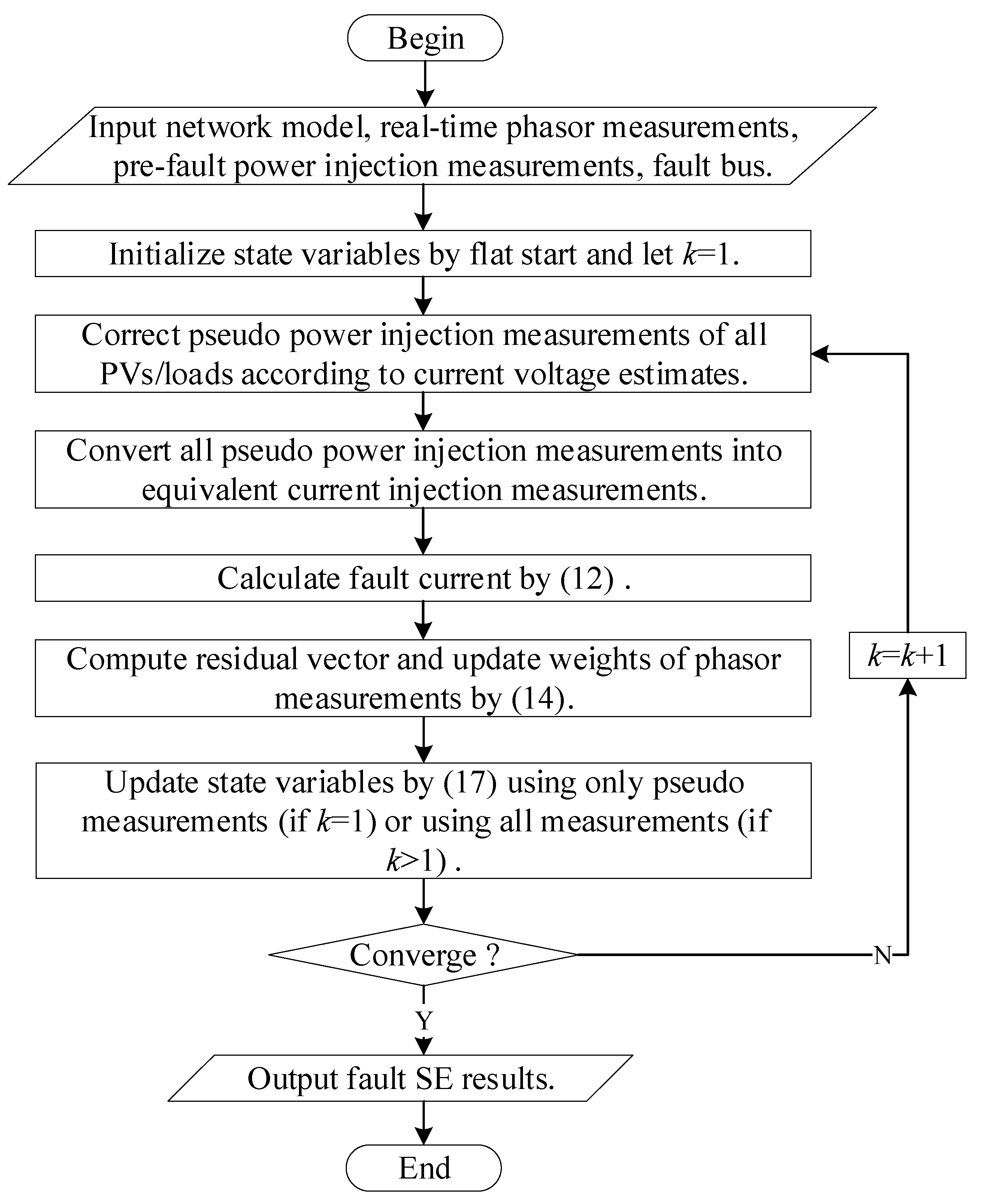
2.2. Three-Phase Fault SE

2.2.1. Correction of Pseudo-PV Power Injection Measurements Under Fault Conditions

Under normal operation, PV systems typically employ maximum power point tracking (MPPT) control to maximize power generation. However, during grid faults, the voltage sag caused by fault currents can significantly impact the power output characteristics. The real power output under fault conditions depends on the control strategy implemented. In the simulations, we follow the “PVSystem” element in OpenDSS and assume that the model of PVs reverts to a constant impedance model if the voltage magnitude sags below a specified threshold. When the voltage sag remains within a certain allowable range, the PV system can maintain its power output through controlled adjustments. Conversely, if the voltage continues to decrease beyond this range and the PV system is equipped with low-voltage ride-through (LVRT) capability, its real power output becomes approximately inversely proportional to the square of the voltage magnitude:

$$P_f=\eta P+(1-\eta )P{\left({\displaystyle \frac{V_f}{V_N}}\right)}^2$$

(9)

where $P,P_f$ are the real power outputs of the PV bus before and during the fault, respectively; $V_f$ is the voltage magnitude at the PV bus during the fault; $V_N$ is the rated system voltage; and $\eta$ is the constant power capability coefficient of the PV system.

Therefore, the pre-fault pseudo power injection measurements of PV buses cannot be directly utilized in SE during fault conditions. To ensure estimation accuracy, these pseudo power injection measurements should be dynamically corrected through successive SE iterations according to the current voltage magnitude estimates of the PV bus:

$$P_{i,\phi ,PV}^{(k)}=\eta P_{i,\phi ,PV}+(1-\eta )P_{i,\phi ,PV}{\left({\displaystyle \frac{V_{i,\phi ,PV}^{(k)}}{V_N}}\right)}^2$$

(10)

where $P_{i,\phi ,PV}$ denotes the rated active power injection measurement at phase φ of the PV bus i; $P_{i,\phi ,PV}^{(k)}$ is the corrected real power injection measurement at phase φ of the PV bus i during the k-th iteration; and $V_{i,\phi ,PV}^{(k)}$ is the voltage magnitude at phase φ of the PV bus i during the k-th iteration.

2.2.2. Correction of Pseudo-Load Power Measurements Under Fault Conditions

Integrated loads are typically characterized using ZIP models. During fault events, the voltage sag at the point of common coupling (PCC) induces significant variations in load power consumption. Consequently, pre-fault pseudo-measurement values for load buses become invalid for SE under fault conditions. This necessitates dynamic correction of pseudo power measurements through successive SE iterations based on the estimated voltage magnitude at the load bus:

$$\begin{array}{l}{P}_{i,\phi ,L}^{(k)}=P_{i,\phi ,L}\left[{\alpha }_1{\left({\displaystyle \frac{V_{i,\phi ,L}^{(k)}}{V_N}}\right)}^2+{\beta }_1{\displaystyle \frac{V_{i,\phi ,L}^{(k)}}{V_N}}+{\gamma }_1\right]\\ Q_{i,\phi ,L}^{(k)}=Q_{i,\phi ,L}\left[{\alpha }_2{\left({\displaystyle \frac{V_{i,\phi ,L}^{(k)}}{V_N}}\right)}^2+{\beta }_2{\displaystyle \frac{V_{i,\phi ,L}^{(k)}}{V_N}}+{\gamma }_2\right]\end{array}$$

(11)

where $P_{i,\phi ,L}^{(k)}$, $Q_{i,\phi ,L}^{(k)}$ are the corrected real and reactive power consumption measurements at phase φ of load bus i during the k-th iteration, respectively; ${\alpha }_1$, ${\beta }_1$, and ${\gamma }_1$ are the coefficients of the constant impedance, constant current, and constant power portions of the active power load, respectively, ${\alpha }_1+{\beta }_1+{\gamma }_1=1$; and ${\alpha }_2$, ${\beta }_2$, and ${\gamma }_2$ are the coefficients of the constant impedance, constant current, and constant power portions of the reactive power load, respectively, ${\alpha }_2+{\beta }_2+{\gamma }_2=1$.

2.2.3. Fault Current Compensation During Ground Fault Conditions

Another distinction between the fault-condition SE and conventional SE stems from system grounding characteristics. In effectively grounded systems, ground fault occurrence establishes a conductive path through the earth to the power source, inducing a fault current at the fault location. This phenomenon alters the network current distribution, and the fault current magnitude varies depending on the unknown fault resistance. To address this issue, a μPMU is deployed at the root bus to measure the complex branch current of the whole feeder. Then, through successive estimation iterations, the fault node current injection can be estimated by subtracting the load-consumed currents of all other buses from the root bus current injection. The estimated fault current is then superimposed to the original pseudo current consumption measurements of the fault point:

$$I_{f,\phi }^{(k)}=I_{1,\phi }^{(k)}-{\displaystyle \sum _{i=2}^n{I}_{i,\phi }^{(k)}}$$

(12)

where $I_{f,\phi }^{(k)}$ is the extracted fault current at phase φ of the fault bus f during the k-th iteration; and $I_{i,\phi }^{(k)},I_{1,\phi }^{(k)}$ are the current injections at phase φ of bus i and the root bus during the k-th iteration, respectively.

Since the fault type is unknown at the time of occurrence, the fault current can be calculated separately for each phase. For example, if a single-phase-to-ground fault occurs at phase A, the iterative process converges such that the fault currents for phase B and C will asymptotically approach zero, thereby identifying phase A as the faulted phase. Thus, this SE-based approach not only identifies the fault type, but also ensures the algorithm’s immunity to fault resistance.

3. Robust Three-Phase Fault SE-Based Fault Localization

Two types of measurements are used in SE: real-time voltage phasor measurements and pseudo-measurements. Pseudo-measurements are derived from pre-fault SE results and assigned low weights, assuming that no incorrect data exist in these values. During fault conditions, however, voltage measurements are subject to disturbances, including time synchronization errors and electromagnetic noise interference under large short-circuit currents. These factors induce non-Gaussian errors, violating the Gaussian error assumption inherent in conventional SE frameworks and leading to faulty estimates. A key challenge arises in identifying these bad measurements. Under normal operation, voltage values remain near 1.0 p.u., enabling simple bad data detection through large deviation checks. During faults, however, fault-induced voltage distortions overlap with measurement anomalies as the faulted feeder experiences an unpredictable voltage sag determined by the unknown fault type, location, and resistance. Consequently, conventional pre-screening methods cannot reliably distinguish genuine fault responses from corrupted measurements. To address this challenge, this section proposes a robust three-phase SE method for reliable fault localization.

3.1. Robust Three-Phase Fault SE

When gross errors are present, robust estimation serves as a complement to conventional estimation theory and possesses three key properties:

• Efficiency: Under the assumed measurement model, the estimation should be optimal or nearly optimal.
• Stability: When there is a slight deviation between the actual measurement model and the assumed model, the estimation should be minimally affected.
• Breakdown resistance: When there is a significant deviation between the actual measurement model and the assumed model, the estimation should not suffer from catastrophic failure.

In this paper, the generalized maximum likelihood estimation (M-estimation) is used for robust fault SE. The robust SE using the M-estimation criterion is constructed as follows:

$$\min J(\mathit{x})={\displaystyle \mathit{\sum }_{i=1}^m\rho (r_i)}$$

(13)

where $r_i=z_i-h_i(\mathit{x})$ is the residual of the i-th measurement; $\rho (\cdot )$ is the penalty function, selected as the quadratic-constant (QC) function [19]:

$$\rho (r_i)=\left\{\begin{array}{l}{r}_i^2/2 \left|r_i\right|\le \beta \\ {\beta }^2 \left|r_i\right|>\beta \end{array}\right.$$

(14)

where β is the tuning parameter. Considering that the pseudo-measurements used in distribution systems have significant noise, the parameter β should not be set too small to avoid interference with the algorithm. Moreover, the fault location method based on comparative matching indices inherently possesses a certain degree of robustness and can tolerate minor incorrect data. Taking these factors into account, β can be set around 1% of the system voltage level. Within this range, the algorithm can avoid interference from pseudo-measurement noise while ensuring that fault location accuracy is not severely compromised.

The IRLS algorithm is employed to solve the model. Setting the first-order partial derivative of the objective function to 0 yields the following [20]:

$$\begin{array}{l}{\displaystyle \frac{\partial J}{\partial \mathit{x}}}={\left({\displaystyle \frac{\partial \mathit{r}}{\partial \mathit{x}}}\right)}^{\mathrm{T}}{\displaystyle \frac{\partial J}{\partial \mathit{r}}}\\ =-{\mathit{H}}^{\mathrm{T}}\mathit{W}\mathrm{diag}(\phi (r_i))=-{\mathit{H}}^{\mathrm{T}}\mathit{W}\mathrm{diag}(\phi (r_i)/r_i)\mathit{r}\\ =-{\mathit{H}}^{\mathrm{T}}\mathit{W}\mathrm{diag}(\varphi (r_i))\mathit{r}=-{\mathit{H}}^{\mathrm{T}}\mathit{W}\mathit{\Phi }(\mathit{r})\mathit{r}=0\end{array}$$

(15)

where $\mathit{\Phi }(\mathit{r})=\mathrm{diag}(\varphi (r_i))$ is the weighting factor matrix; $\mathit{r}=\mathit{z}-\mathit{h}(\mathit{x})\in {ℝ}^{m\times 1}$ is the residual vector; $\mathit{W}={\mathit{R}}^{-1}$ is the initial weight matrix; and $\phi (r_i)$ and the weighting factor $\varphi (r_i)$ are given by the following:

$$\phi (r_i)={\displaystyle \frac{\partial \rho (r_i)}{\partial r_i}}=\left\{\begin{array}{l}{r}_i \left|r_i\right|\le \beta \\ 0 \left|r_i\right|>\beta \end{array}\right., \varphi (r_i)={\displaystyle \frac{\phi (r_i)}{r_i}}=\left\{\begin{array}{l}1 \left|r_i\right|\le \beta \\ 0 \left|r_i\right|>\beta \end{array}\right.$$

(16)

The Gauss–Newton method is used to iteratively solve the nonlinear equation system (15), and the correction equation for the state vector at the k-th iteration is given by the following:

$$\Delta {\mathit{x}}^{(k)}={[{\mathit{H}}^{\mathrm{T}}\mathit{\Phi }({\mathit{x}}^{(k)})\mathit{H}]}^{-1}{\mathit{H}}^{\mathrm{T}}\mathit{\Phi }({\mathit{x}}^{(k)})[\mathit{z}-\mathit{h}({\mathit{x}}^{(k)})]$$

(17)

Note that the weighting factors of pseudo-measurements are always fixed at 1.0, while those of real-time phasor measurements are dynamically updated based on their residual values during iterations. In each iteration, if the residual falls within a certain range, the phasor measurement is considered accurate and its weighting factor is set to 1.0. When the absolute value of the residual exceeds a certain threshold, the weighting factor of the corresponding phasor measurement is set to 0. In this way, the negative effect of bad phasor measurements is eliminated.

The flowchart of the robust fault SE algorithm is shown in Figure 1. It is critical to emphasize that, given the inherently low measurement redundancy in distribution networks, an additional strategy is implemented in the algorithm: during the initial iteration, state variables are exclusively updated using pseudo-measurements. Phasor measurements are deliberately deferred to subsequent iterations. This strategic ensures robustness, as dynamically adjusting phasor measurement weights in the first iteration risks allowing incorrect data to dominate the residual distribution, leading to the erroneous discarding of normally distributed measurements in subsequent iterations. Finally, the algorithm’s robustness depends on measurement redundancy: when more μPMUs are configured, it becomes more robust to incorrect data due to higher measurement redundancy; conversely, with limited μPMUs, it can only tolerate lower contamination rates.

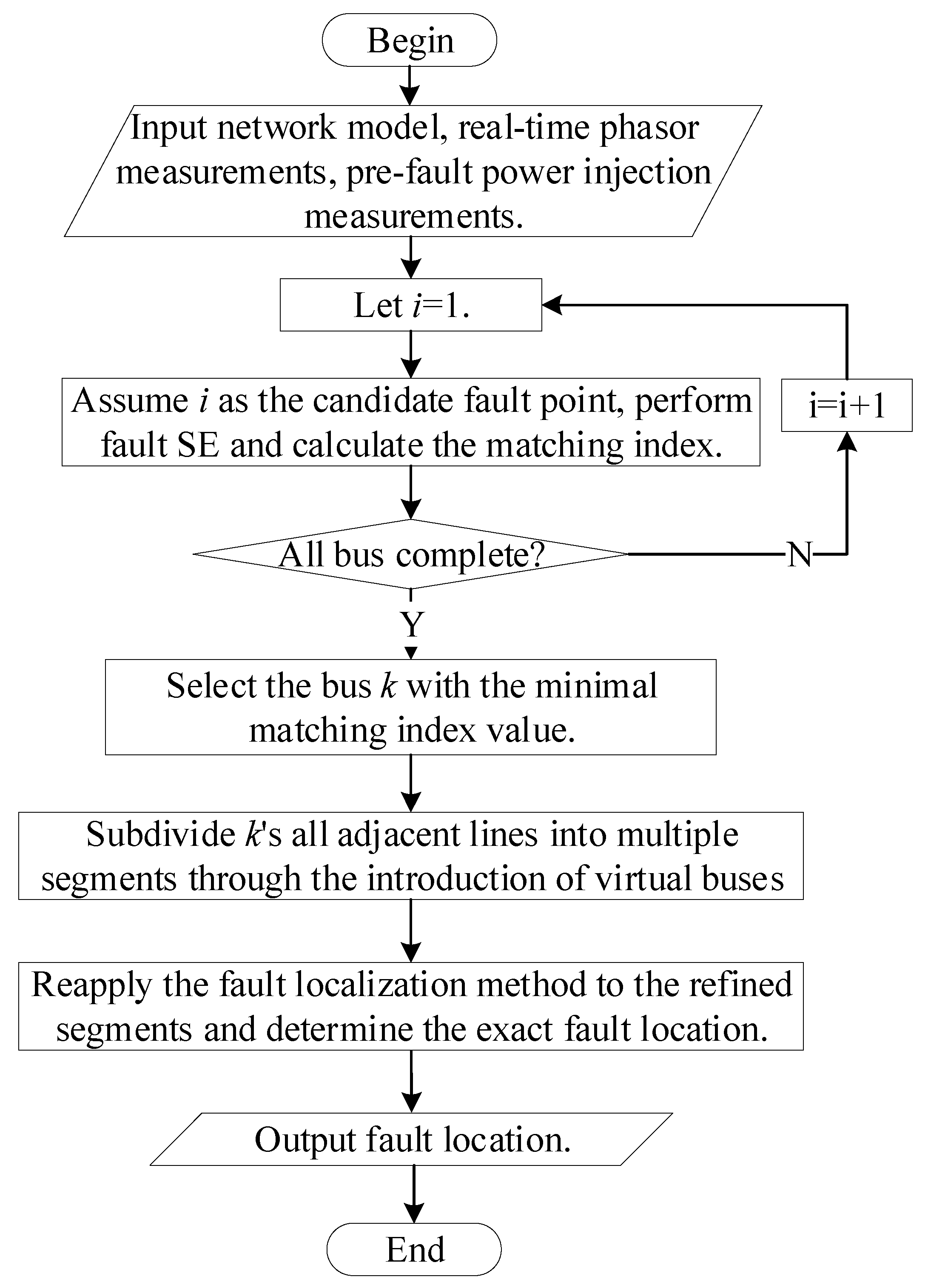
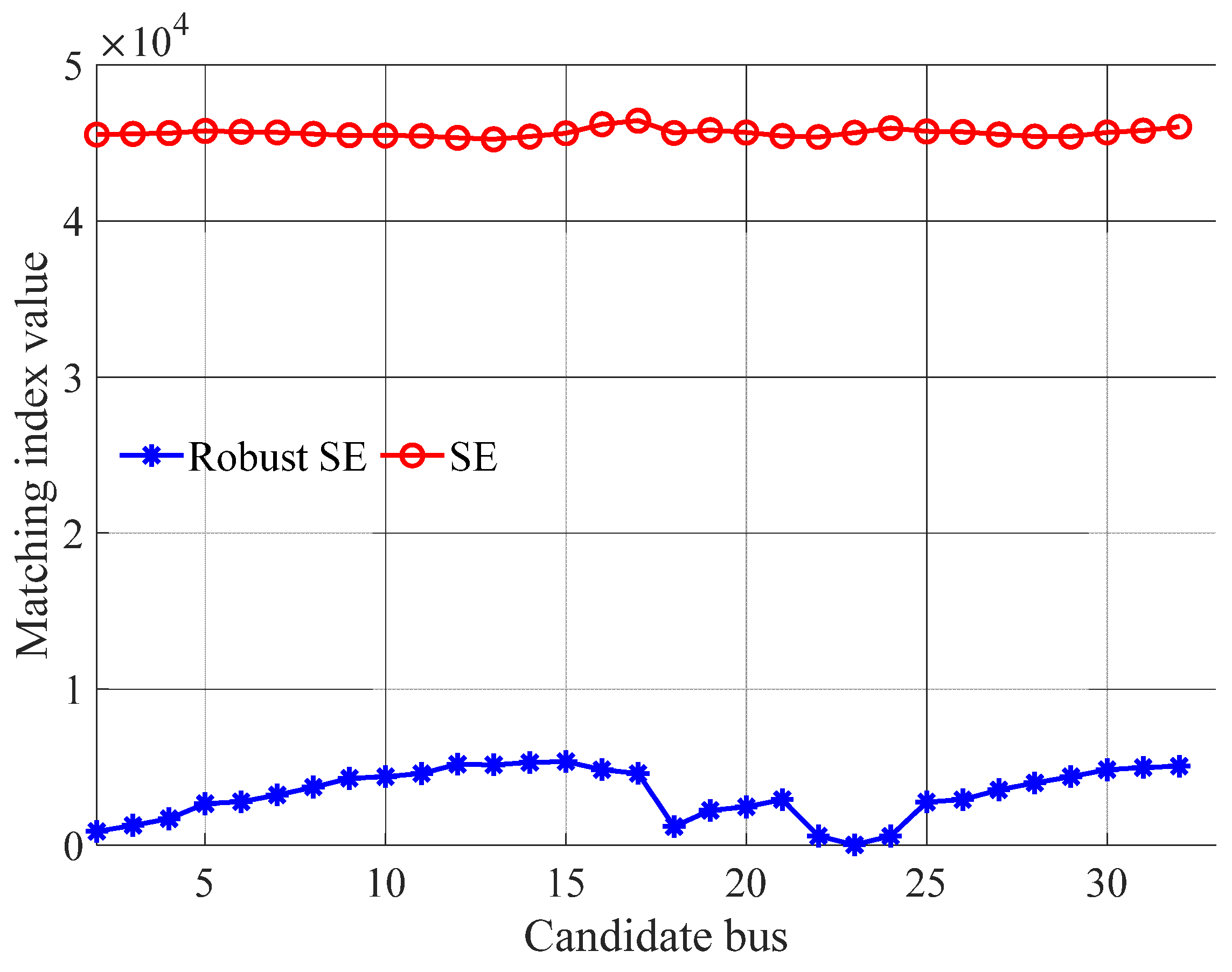
3.2. Robust SE-Based Fault Node Localization

The fault localization algorithm is based on the principle that faults at different positions create different voltage sag. The implementation process follows these steps: (1) Assume a candidate fault location. (2) Perform fault SE while injecting the calculated fault current into this candidate bus during each iteration. (3) Compute a matching index after SE convergence at the current candidate location. This procedure repeats cyclically until all potential fault locations have been systematically evaluated.

The matching index for a candidate fault node i consists of two terms:

$$FL(i)={‖\mathit{z}-\mathit{h}(\widehat{\mathit{x}})‖}_{\mathit{\Phi }}^2+{\displaystyle \sum _{i\in {\Omega }_{end}}{\displaystyle \sum _{\phi \in \{a,b,c\}}\left|V_{i,\phi }^{meas}-V_{i,\phi }^{est}\right|}}$$

(18)

where $\widehat{\mathit{x}}$ is the estimated value of the state variable; the norm is defined as $\left|\right|\mathit{a}|{|}_{\mathit{Z}}^2={\mathit{a}}^{\mathrm{T}}\mathit{Z}\mathit{a}$; $V_{i,\phi }^{meas}$ and $V_{i,\phi }^{est}$ are the measured and estimated values of the voltage amplitude at phase φ of the remote end bus i, respectively; and ${\Omega }_{end}$ is the set of all remote terminal buses.

The design of the two terms is illustrated as follows:

(1)

The first term is the L₂ norm of the measurement residual vector, excluding phasor measurements with zero weighting factors. Since the weights of phasor measurements and pseudo-measurements differ significantly, the initial weight matrix W is not considered to prevent a situation where the large disparity in weights causes one type of measurement residuals dominate the matching index, thereby masking the characteristics of the other type of measurement residuals.

(2)

The second term is the L₁ norm of the residual vector of voltage magnitude measurements specifically at remote-end buses of distribution laterals. These voltage magnitude measurements come from low-cost smart meters and do not participate in SE as the nonlinear relation with state variables make the Jacobian matrix no longer constant. However, if μPMUs are configured at these buses, the phasor measurements they provide can be incorporated into the SE, and the second term can be dropped to simplify the formulation.

After calculating the matching index values for all candidate fault nodes, the node with the lowest matching index value is selected as one endpoint of the faulted line:

$$\widehat{i}=\arg \underset{i}{\min }FL(i)$$

(19)

Upon identifying the bus with the minimum matching index, its adjacent lines are subdivided into multiple segments through the introduction of corresponding virtual buses. Reapplying the fault localization methodology to these refined segments enables precision improvements in fault identification. For each fault SE, the system’s admittance matrix undergoes dimension expansion to accommodate the added virtual buses. Concurrently, the measurement vector is extended by incorporating zero-injection measurements at these virtual buses, while the state vector is augmented with voltages of the virtual buses. This approach enables more precise fault localization. The fault localization algorithm is illustrated in Figure 2.

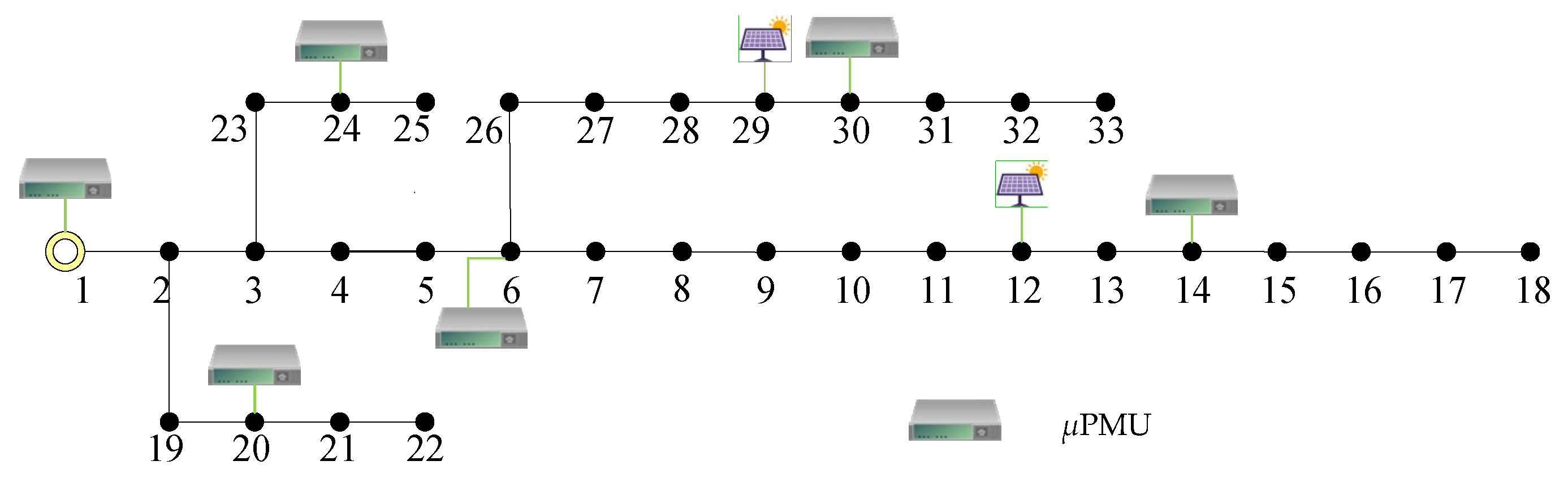
3.3. Measurement Configuration

If there is no voltage magnitude measurement downstream of the fault point; the SE-matching-based fault localization method fails to identify a faulted line if no voltage measurement exists at downstream of the fault. This is illustrated as follows. Assume a fault occurs at the downstream of a bus i with a voltage magnitude meter configured:

• If the assumed tentative bus is also at the downstream of bus i, then the compensated fault current always flows through the path from the root bus to bus i. It is easy for the SE algorithm to make the estimated voltage magnitude of bus i close to the measured value, regardless of which downstream bus is assumed. Therefore, it is impossible to distinguish which downstream bus is a terminal bus of the true faulted line.
• If the assumed tentative bus is at the upstream of bus i, then the compensated fault current only flows through a part of the path from the root bus to bus i. The estimated voltage value of bus i tends to be greater than the measured value. Being unable to minimize the overall objective function value, the SE algorithm will try to increase the pseudo-measurements’ residuals to reduce the voltage magnitude measurement’s residual. In other words, the high pseudo measurement residuals are the cost that must to be paid for accurately fitting of the voltage magnitude measurement. The further away the assumed tentative bus is from the fault point, the larger the cost (the first term in (18)) that needs to be paid. In this case, it is possible to distinguish which upstream bus is a terminal bus of the true faulted line.

4. Simulation Results

In this section, the proposed method is evaluated on a 33-bus distribution network with a voltage level of 12.66 kV.

The original system is extended to an unbalanced three-phase network incorporating single-phase loads, as illustrated in Figure 3. Two PV generators are installed at buses 12 and 29. All loads are modeled as constant impedance. The placement of μPMUs is determined through offline optimization using a genetic algorithm, aiming to maximize the fault localization success rate, under the assumption that there are no incorrect data and that the total number of μPMUs is fixed. Consequently, there were six μPMUs at buses 1, 6, 14, 20, 24, and 30, with pseudo-measurements applied to all buses. The single-phase load capacities range from 60 kW + j20 kVar to 200 kW + j100 kVar. The neutral point of the transformer at bus 1 is solidly grounded. Simulations are implemented in OpenDSS [21]. The maximum number of iterations for SE was set to 20. Since the algorithm operates in actual voltage values rather than per-unit representation, a convergence threshold of max (Δx) < 0.1 V prove to be sufficient to achieve satisfactory accuracy within 3~4 iterations for the 33-bus system (12.66 kV nominal voltage), while substantially lowering computational requirements. On the other side, the variations in matching index values resulting from fault current injection at different candidate locations are substantially greater than the minor estimation errors introduced by slightly relaxed convergence criteria. Therefore, this convergence criteria is acceptable for the fault localization task.

4.1. Typical Scenario Testing

This section evaluates the performance of the SE-based fault localization method under a typical scenario. An AB-phase-to-ground short-circuit fault is simulated at bus 24 with a fault resistance of 10 Ω to simulate practical moderate-impedance fault scenarios. All measurements are generated by superimposing Gaussian errors to their true values. The relative error of pseudo power injection, voltage magnitude, and current magnitude measurements are set to 5%, 0.4% and 0.0016%, respectively, while the absolute error of voltage phase angle and current phase angle measurements are set to 1 × 10⁻³ rad and 5.8 × 10⁻³ rad, respectively [16]. β is set to 100.

To validate the robustness of the proposed robust SE-based fault localization methodology, incorrect data are intentionally introduced by scaling the three-phase voltage magnitude measurements of a randomly selected μPMU to 45~55% of their true values, resulting in totally six incorrect data including real and imaginary parts. The fault localization algorithm leveraging robust SE is then applied to assess its immunity to data anomalies. For comparative analysis, a conventional SE-based fault localization method is concurrently tested.

Figure 4 illustrates the matching index values across candidate buses derived from both approaches. The results demonstrate that the robust SE method achieves a minimum matching index at bus 24, accurately pinpointing the true fault location while mitigating the impact of corrupted measurements. In contrast, the conventional SE method produces significantly distorted matching indices across suspected fault buses, failing to converge on a definitive fault location due to its vulnerability to measurement outliers.

4.2. Comprehensive Multi-Scenario Testing

This section rigorously evaluates the line fault localization capability of the proposed algorithm through a systematic testing framework. A total of 310 fault scenarios are simulated across all lines except line 1–2, encompassing ten distinct fault types: single-phase-to-ground faults (A-g, B-g, C-g), two-phase-to-ground faults (AB-g, BC-g, AC-g), two-phase faults (AB, BC, AC), and three-phase faults (ABC). Fault locations are randomized between 10~90% of each line’s length from the starting bus, with three fault resistance ranges tested: 0~100 Ω, 0~200 Ω, and 0~500 Ω. The relative errors of pseudo power injection measurements vary in range 5~50%.

To stress-test robustness, artificial incorrect data are generated by scaling three-phase voltage magnitude measurements from a randomly selected μPMU to 25~35%, 45~55%, or 75~85% of their true values. For each of the 310 fault scenarios, the evaluation adopts terminal node identification as the success criterion for operational practicality, requiring the algorithm to detect at least one endpoint of the faulted line. For instance, a fault occurring 75% along line 6~7 segment would be considered successfully localized if either bus 6 or 7 is identified, balancing precision requirements with maintenance crew workflows.

Figure 5 compares the fault localization performance of conventional SE and the proposed robust SE method across multiple test scenarios. As illustrated in Figure 5a, under ideal measurement conditions without incorrect data, both methods demonstrate similar success rates. However, their performance deteriorates as pseudo-measurement errors increase, with larger fault resistances (e.g., above 200 Ω) and higher pseudo-measurement errors (e.g., above 30%), exacerbating the decline in localization accuracy. High-impedance faults (HIFs) are challenging to locate due to their extremely weak fault characteristics. While SE-based methods theoretically possess HIF localization capability given accurate measurements, their performance deteriorates significantly under high pseudo-measurement noise or gross errors in μPMU data. However, it is observed that both SE-based methods achieves 90% localization accuracy with noise-free data and maintains functionality (albeit with two-hop neighborhood deviations) under noisy measurements.

A critical distinction arises in scenarios with measurement contamination. Conventional SE-based localization fails completely when incorrect data are present, rendering it incapable of identifying fault locations. In contrast, the robust SE method maintains high effectiveness even under severe data corruption: it achieves a 90% success rate despite simultaneous challenges, including 20% relative errors in pseudo-power injection measurements, high-resistance faults (up to 200 Ω), and the contamination of 20% erroneous voltage measurements. Notably, the method demonstrates stable performance under measurement value deterioration, showing only a 5% success rate reduction when erroneous measurements degrade from 0.8 to 0.4. This controlled accuracy attenuation persists even under high fault-resistance conditions (200 Ω), validating its resilience to uncalibrated measurement distortions while maintaining fault signature detectability.

4.3. Comparative Tests Between Robust SE-Based and AI-Based Fault Localization Methods

To verify the fault localization capability of the proposed robust SE method when dealing with incorrect data in real-time measurements, we conducted comparative tests using AI-based approaches, first by designing a graph neural network (GNN)-based fault localization framework. The GNN-based framework proposed in this paper consists of three stages. Stage 1 is the graph embedding phase, which uses a concatenation-based aggregation GNN model to enhance the information embedding capability for unobservable nodes in the network. Stage 2 employs an attention network to perform fault localization and fault-type identification under supervised learning. Its structure is shown in Figure 6.

Meanwhile, 49,446 samples of pre-fault active and reactive power loads at all buses are generated by sampling from a Gaussian mixture model, which is learned from realistic data. Five levels of fault resistance are configured, and faults are simulated on each line following the same methodology as in Section 4.2. Subsequently, three-phase voltage magnitudes and phase angles are extracted from instrumented measurement buses, with measurement errors added at the same level as described in Section 4.2. The dataset is then divided into training, validation, and test sets. In the test set, three-phase voltage phasor measurements of one randomly selected μPMU are corrupted to simulate incorrect data, in order to evaluate the robustness of AI-based methods against such data. Additionally, we set the error of pseudo-measurements used in robust SE to 25%. The evaluation adopts terminal node identification as the success criterion. The test results are shown in

Table 1. Comparison of SE, robust SE, and GNN-based fault localization methods.

Method	Different Fault Resistance Levels
	0~100 Ω	0~200 Ω	0~500 Ω
SE	14.4%	12.5%	11.7%
Robust SE	95.5%	87.6%	75.3%
GNN	67.1%	56.9%	42.2%

.

AI-based methods demonstrate a certain degree of resilience to incorrect data and perform better than traditional SE-based methods. However, their performance is significantly inferior to that of robust SE methods. This is because the proposed method builds a comprehensive robust SE model, whereas AI-based approaches can only rely on their generalization capability to handle data deviations. More importantly, AI-based methods require a large number of fault samples for offline training to achieve acceptable performance, leading to significant computational resources. On the other side, if the training dataset lacks sufficient diversity and fails to cover scenarios in the test set, the fault localization accuracy of AI-based methods is reduced.

In summary, the proposed method, from the perspective of resisting incorrect data, integrates a robust SE model into a SE-based fault localization approach. It suppresses incorrect data in real-time measurements by leveraging redundant pseudo-measurements. Additionally, the method does not require extensive fault sample training, making it more straightforward and efficient.

5. Conclusions

To address the limitation that conventional SE-based methods fail to differentiate authentic fault responses from measurement distortions due to uncertainties in fault types, locations, and resistances, a robust three-phase SE-driven fault localization methodology is proposed, leveraging real-time voltage phasor measurements and pseudo-measurements derived from pre-fault SE results. A robust fault SE model is built using the quadratic-constant-based generalized maximum likelihood estimation and is solved using the iteratively reweighted least squares algorithm with adaptive measurement weighting. Furthermore, a fault SE matching-based fault localization algorithm is proposed through the systematic traversal of candidate buses, where each potential fault location is evaluated by performing the robust-fault SE.

The effectiveness of the proposed algorithm is validated through thorough simulation analysis on a 33-bus unbalanced distribution network, with the following conclusions:

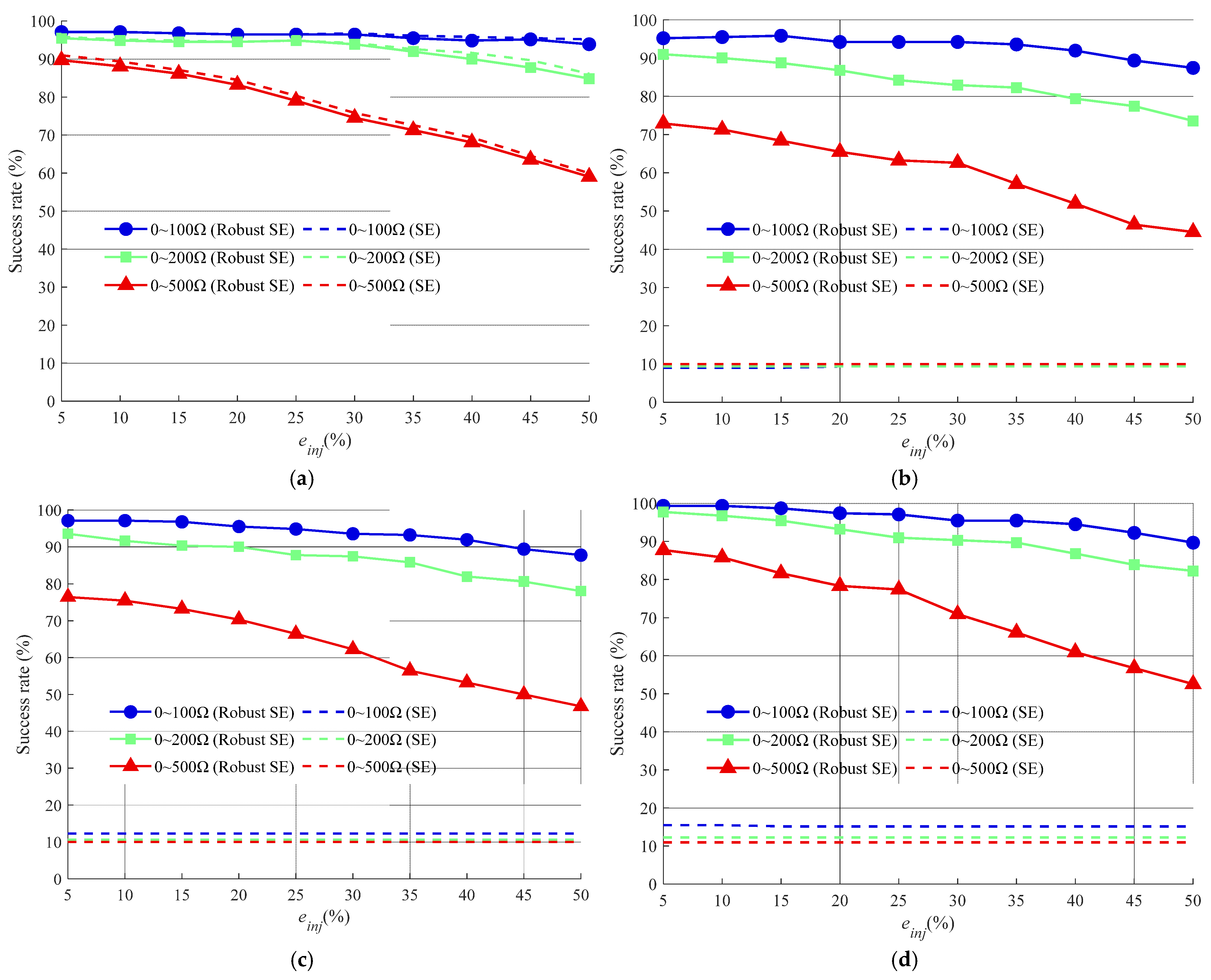
• Under ideal measurement conditions without incorrect data, the robust SE-based method demonstrates similar performance to the conventional SE-based method. Consequently, the proposed approach can be integrated into various existing SE-based fault localization methods to enhance their robustness against incorrect data.
• The robust SE-based method maintains high effectiveness even under severe data corruption, while the conventional SE-based localization fails completely. Specifically, it achieves a 90% success rate despite simultaneous challenges, including 20% relative errors in pseudo-power injection measurements, high-resistance faults (up to 200 Ω), and the contamination of 20% erroneous voltage measurements.
• The method demonstrates stable performance under measurement value deterioration. Specifically, it shows only a 5% success rate reduction when erroneous measurements degrade from 0.8 to 0.4. This controlled accuracy attenuation persists even under high fault-resistance conditions (200 Ω), validating its resilience to uncalibrated measurement distortions while maintaining fault signature detectability.
• The proposed robust SE-based fault localization method demonstrates a superior incorrect data rejection capability compared to GNN-based approaches. Furthermore, it eliminates the need for extensive fault sample training, exhibiting stronger adaptability.

While the proposed method enhances fault localization robustness, it currently faces three limitations: dependency on precise network parameters, scalability challenges in large systems, and exclusive reliance on steady-state measurements. Future research will develop integrated parameter/topology identification techniques, fast pre-screening mechanisms to reduce computational burden, and hybrid dynamic-static SE techniques to leverage multi-scale measurement data.

References

1. Abdalla, O.H.; Mostafa, A. Optimal number and locations of smart RMUs for self-healing distribution networks. Int. Trans. Electr. Energy Syst. 2022, 2022, 4819129. [Google Scholar] [CrossRef]
2. Mirshekali, H.; Dashti, R.; Keshavarz, A.; Torabi, A.J.; Shaker, H.R. A novel fault location methodology for smart distribution networks. IEEE Trans. Smart Grid 2021, 12, 1277–1288. [Google Scholar] [CrossRef]
3. Tashakkori, A.; Wolfs, P.J.; Islam, S.; Abu-Siada, A. Fault location on radial distribution networks via distributed synchronized traveling wave detectors. IEEE Trans. Power Deliv. 2020, 35, 1553–1562. [Google Scholar] [CrossRef]
4. Chen, B.C.; Yu, N.; Chen, B.; Tian, C.H.; Chen, Y.J.; Chen, G.R. Fault location for underground cables in ungrounded MV distribution networks based on ZSC signal injection. IEEE Trans. Power Deliv. 2021, 36, 2965–2977. [Google Scholar] [CrossRef]
5. Stipetic, N.; Filipovic-Grcic, B.; Ziger, I. LF signal injection for earth-fault localization in unearthed distribution network. Electr. Power Syst. Res. 2023, 220, 109249. [Google Scholar] [CrossRef]
6. Yang, M.; Liu, Y.; Guo, L.; Wang, Z.; Zhu, J.; Zhang, Y.; Cheng, B.; Wang, C. Hierarchical distributed chance-constrained voltage control for HV and MV DNs based on nonlinearity-adaptive data-driven method. IEEE Trans. Power Syst. 2025, 40, 806–819. [Google Scholar] [CrossRef]
7. Ge, L.; Liu, H.; Yan, J.; Sun, B.; Li, Y.; Hou, L. A novel distributed PV data virtual collection with continuous-binary denoising auto-encoders. IEEE Trans. Smart Grid 2024, 15, 1152–1164. [Google Scholar] [CrossRef]
8. Li, W.T.; Deka, D.; Chertkov, M.; Wang, M. Real-Time faulted line localization and PMU placement in power systems through convolutional neural networks. IEEE Trans. Power Syst. 2019, 34, 4640–4651. [Google Scholar] [CrossRef]
9. Guo, M.F.; Yang, N.C.; Chen, W.F. Deep-learning-based fault classification using Hilbert-Huang transform and convolutional neural network in power distribution systems. IEEE Sens. J. 2019, 19, 6905–6913. [Google Scholar] [CrossRef]
10. Rizeakos, V.; Bachoumis, A.; Andriopoulos, N.; Birbas, M.; Birbas, A. Deep learning-based application for fault location identification and type classification in active distribution. Appl. Energy 2023, 338, 120932. [Google Scholar] [CrossRef]
11. Mirshekali, H.; Keshavarz, A.; Dashti, R.; Hafezi, S.; Shaker, H.R. Deep learning-based fault location framework in power distribution grids employing convolutional neural network based on capsule network. Electr. Power Syst. Res. 2023, 223, 109529. [Google Scholar] [CrossRef]
12. Jamei, M.; Ramakrishna, R.; Tesfay, T.; Gentz, R.; Roberts, C.; Scaglione, A.; Peisert, S. Phasor measurement units optimal placement and performance limits for fault localization. IEEE J. Sel. Areas Commun. 2020, 38, 180–192. [Google Scholar] [CrossRef]
13. Al-Hinai, A.; Karami-Horestani, A.; Alhelou, H.H. A multi-objective optimal PMU placement considering fault-location topological observability of lengthy lines: A case study in OMAN grid. Energy Rep. 2023, 9, 1113–1123. [Google Scholar] [CrossRef]
14. Sheta, A.N.; Abdulsalam, G.M.; Eladl, A.A. Online tracking of fault location in distribution systems based on PMUs data and iterative support detection. Int. J. Electr. Power Energy Syst. 2021, 128, 106793. [Google Scholar] [CrossRef]
15. Pignati, M.; Zanni, L.; Romano, P.; Cherkaoui, R.; Paolone, M. Fault detection and faulted line identification in active distribution networks using synchrophasors-based real-time state estimation. IEEE Trans. Power Deliv. 2017, 32, 381–392. [Google Scholar] [CrossRef]
16. Gholami, M.; Abbaspour, A.; Moeini-Aghtaie, M.; Fotuhi-Firuzabad, M.; Lehtonen, M. Detecting the location of short-circuit faults in active distribution network using PMU-based state estimation. IEEE Trans. Smart Grid 2020, 11, 1396–1406. [Google Scholar] [CrossRef]
17. Zhang, Y.; Wang, J.H.; Khodayar, M.E. Graph-based faulted line identification using micro-PMU data in distribution systems. IEEE Trans. Smart Grid 2020, 11, 3982–3992. [Google Scholar] [CrossRef]
18. Pegoraro, P.A.; Sitzia, C.; Solinas, A.V.; Sulis, S.; Carta, D.; Benigni, A. Compensation of systematic errors for improved PMU-based fault detection and location in three-phase distribution grids. IEEE Trans. Instrum. Meas. 2024, 73, 9003712. [Google Scholar] [CrossRef]
19. Abur, A.; Exposito, A.G. Power System State Estimation: Theory and Implementation; CRC Press: Boca Raton, FL, USA, 2004. [Google Scholar]
20. Su, S.; Liang, D.; Zeng, L.; Wang, X. Robust state estimation of integrated electricity gas systems based on constrained iteratively reweighted least squares. In Proceedings of the 2023 International Conference on Power System Technology (PowerCon), Jinan, China, 21–22 September 2023; pp. 1–6. [Google Scholar]
21. Dugan, R.C.; McDermott, T.E. IEEE In An open source platform for collaborating on smart grid research. In Proceedings of the 2011 IEEE Power and Energy Society General Meeting, Detroit, MI, USA, 24–28 July 2011. [Google Scholar]
Figure 1. Flowchart of robust-fault SE algorithm.
Energies 18 02551 g001
Figure 2. Flowchart of the fault SE-based fault localization algorithm.
Energies 18 02551 g002
Figure 3. Single-line diagram of the 33-bus distribution network.
Energies 18 02551 g003
Figure 4. Matching index value comparison of different candidate buses using SE and robust SE-based fault localization methods.
Energies 18 02551 g004
Figure 5. Comprehensive multi-scenario testing results comparison using SE and robust SE-based fault localization methods. (a) 1.0; (b) 0.35~0.45; (c) 0.45~0.55; (d) 0.75~0.85.
Energies 18 02551 g005
Figure 6. The neural network structure based on GNN and multi-task learning.
Energies 18 02551 g006