Expansion Planning of Electrical Distribution Systems Considering Voltage Quality and Reliability Criteria

Abstract

This study aimed to assess the power capacity of electrical conductors under the long-term expansion of distribution systems over a 10-year horizon by considering voltage quality constraints and reliability indicators. The MATPOWER library in Matlab was employed, along with the IEEE 15-bus and 33-bus distribution system test cases. A 5% annual load growth was simulated for each system, which involved analyzing key parameters, such as the power loss, voltage deviation, and average failure rate. An algorithm was developed to perform a multi-criteria analysis, which provided optimal solutions for the system behavior in response to increasing demand. Given the close relationship between distribution systems and load growth, voltage quality and reliability indicators were evaluated annually to identify improvement opportunities by taking into account economic factors, implementation timelines, the replacement of electrical components, and medium- and long-term investments. The proposed algorithm recommended upgrades to electrical conductors without significantly affecting the system costs. For the initial year of the IEEE 15-bus system, enhancements were suggested for lines L1–L2, L2–L3, L3–L4, L2–L6, L3–L11, and L11–L12, which allowed the system to operate without further modifications for five years, maintained the minimum voltages above 0.95 p.u., and reduced the average failure rate while demand continued to grow.

1. Introduction

The electrical distribution system is responsible for delivering electric power to end users. Before reaching this stage, electricity undergoes generation and transmission processes, making distribution the final step in the power supply chain [1].

The key characteristics of distribution systems include the operating voltage level—typically in the range of 6 kV to 36 kV—used in both urban and rural areas [2], and distribution transformers, which reduce the voltage level to supply electricity safely and efficiently to end users [3].

As the final link in the power supply chain, the distribution system must ensure the reliable, secure, and efficient delivery of energy, maintaining proper power quality in terms of the voltage and frequency [3,4].

Over time, distribution systems must dynamically adapt to increasing demand, considering parameters such as reliability, stability, and quality [5].

The power quality in a distribution system refers to its ability to deliver electricity in conditions suitable for use, without disturbances that may negatively affect end users [5,6]. The key parameters used to evaluate the power quality include the voltage (above 0.95 p.u.), frequency (around 60 Hz), flicker (rapid voltage variations), and interruptions (momentary outages).

Reliability refers to the system’s ability to supply electricity without interruptions or failures for as much time as possible, ensuring constant power availability for users [7]. The most commonly used reliability indicators are the interruption frequency, average failure rate, duration of interruptions, and restoration time [8].

Several factors affect the power quality and reliability in distribution systems, including external weather conditions (e.g., thunderstorms, landslides, or strong winds), poor maintenance (e.g., lack of upkeep for transformers, cables, or substations), overloads (operation beyond capacity), technical or human failures (e.g., operational errors or equipment failures), and outdated infrastructure (e.g., aging systems not designed for growing demand) [9,10].

With technological advancement, electrical engineering continues to offer solutions to emerging power quality and reliability issues. These include protection coordination [10], voltage control through sensor integration [11], and proposals for distributed generation near the distribution network [12].

Likewise, the implementation of systems with neural analysis (intelligent learning) has become increasingly relevant [9], as they can provide solutions based on the data they gather over time. Nevertheless, it is crucial to consider the current condition of distribution systems, especially since investment analysis focused on such systems is often neglected. These investments are essential for system development and growth and include key aspects such as new technologies, communication, sustainability, and resilience [12,13].

Although several methods exist to address the problems related to increasing demand—considering both economic and sustainability aspects—there is a growing need for fast and efficient methods, particularly those based on single- or multi-criteria decision-making functions [14], that are both robust and accurate.

Multi-criteria decision analysis (MCDA) enables the incorporation of multiple criteria to deliver optimal solutions while applying restrictions or initial conditions to the function [15]. The key features of MCDA include evaluation capabilities (allowing for the analysis of several variables—decisions should not rely on a single factor), qualitative or quantitative criteria, trade-offs (balancing between conflicting criteria), and weight assignment (based on each criterion’s relative importance) [16,17].

Decision-making within MCDA depends on the problem context, identification of criteria, weight assignment, number of alternatives, and application domain. Commonly used methods include the Analytic Hierarchy Process (AHP)—which uses pairwise comparisons between criteria and alternatives; Linear Weighting—where weights are multiplied by values for each alternative; and the Technique for Order of Preference by Similarity to Ideal Solution (TOPSIS)—which selects the alternative closest to the ideal solution and farthest from the worst-case scenario. These techniques help balance and prioritize conflicting criteria [18,19].

When properly applied with well-defined criteria and parameter values, MCDA can be used to analyze the performance of a distribution system under increasing demand. This allows for the optimization of power quality, reliability, and economic performance, producing effective results in a reduced amount of time.

2. Methodology

2.1. Impact of Demand Growth

The increase in demand within electrical distribution systems generates significant challenges, such as an increased load on existing infrastructure, the risk of overloading, higher technical losses, and the deterioration of service quality and reliability delivered to end users. In order to mitigate these impacts, the electrical engineering field has proposed various solutions, including the modernization of networks using smart technologies, the integration of renewable energy sources, and active demand-side management through the use of advanced control systems.

However, these methods often entail high economic costs for society and their implementation timelines are not ideal for addressing short-term issues. This has led electrical engineers to consider short-, medium-, and long-term strategies capable of providing optimal and efficient solutions. These approaches are commonly present in short-term preventive actions based on annual demand growth analysis. Such actions include increasing investment in infrastructure, conducting preventive maintenance, and assessing the impact on conductors—measures that contribute to ensuring the sustainability and resilience of the systems in the face of continuous demand growth.

Based on the above, it is necessary to conduct a demand growth analysis using two different scenarios: the IEEE 15-bus case and the IEEE 33-bus case, both of which are associated with distribution system models. Using these templates as study scenarios, the following case study is proposed for each model: analyze the year-by-year behavior of the demand and its potential impacts; verify that the models meet voltage quality and reliability requirements; incorporate the electrical results obtained from increasing demand into a multi-criteria function; derive optimal results through multi-criteria function analysis; integrate these results into the system; and finally, continue with the analysis of the subsequent year until the 10-year study horizon is completed.

2.2. Initial Considerations

Prior to the development of the multi-criteria function in Matlab, it was necessary to obtain essential data for its implementation. These data are related to the active and reactive powers of the loads at each bus, the characteristics of the selected system, line impedance, line losses, the type of associated electrical conductor, and the calculation of its respective length. By applying a reliability parameter (average failure rate) and quality parameter (voltage deviation), the behavior of the distribution system under increasing demand was analyzed.

The distance of the distribution lines is a key parameter to consider, as it directly affects the reliability indicators of the system—specifically, the average failure rate, which serves as the reliability metric in this study. Given the characteristics of distribution systems, conductors are typically made of aluminum or aluminum alloys.

The equation for determining the line distance is as follows:

$$d=(Z\ast \phi )/\rho$$

(1)

where

• d: length of the line in meters (m).
• Z: magnitude of the line impedance in ohms ($\Omega$).
• $\phi$: cross-sectional area of the conductor in square millimeters (mm²).
• $\rho$: resistivity of aluminum, approximately $2.82\times {10}^{-8}$ Ω·m.

Similarly, the nominal current of each conductor in the IEEE bus system models mentioned previously was considered. This allowed for the calculation of the average failure rate per kilometer, assuming a failure occurrence rate between 0.01% and 0.1% annually over 1000 to 10,000 km. The occurrence of failures is also influenced by the environmental conditions surrounding the distribution system; for this analysis, a high-corrosion environment was assumed.

The following equation defines the average failure rate:

$$TFP=(\#F)/(L\ast T\ast CN)$$

(2)

where

• TFP: average failure rate per kilometer (km).
• #F: number of failure events over a given time period.
• L: length of the conductor in kilometers (km).
• T: time period over which the average failure rate is analyzed.
• CN: normalized load, obtained from the ratio between the line current and the conductor’s nominal current, measured in amperes (A).

To assess the system behavior in terms of voltage quality, the voltage deviation equation was implemented and analyzed, considering the annual growth in demand, as shown below:

$$\mathrm{DESV}=\left|1-V_n\right|$$

(3)

where

• DESV: voltage deviation.
• 1: ideal voltage in per unit (p.u.).
• $V_n$: actual voltage in per unit (p.u.) at the bus.

The objective of the voltage deviation analysis was to verify that the measured voltage at each bus remained as close as possible to the ideal value of 1 p.u. In other words, the deviation result should ideally approach zero.

2.3. Future Considerations

For future analyses, reference is made to data available in the Ecuadorian electricity market. The diversity of aluminum conductors allows for data classification based on three main types: All-Aluminum Conductor (AAC), All-Aluminum Alloy Conductor (AAAC), Aluminum Conductor Steel-Reinforced (ACSR), and aluminum–steel alloy combinations. For the present study, the AAC or ASC and ACSR groups are considered, depending on the characteristics and needs of the network. The data used are shown in

Table 1. Electrical conductor data for ASC or AAC model.

Code	Gauge (AWG)	Cross-Sectional Area (mm2)	Resistance (ohm/km)	Price (USD/m)
Peachbell	6	13.3	2.170	0.366
Rose	4	21.15	1.360	0.582
Iris	2	33.62	0.856	0.926
Poppy	1/0	53.49	0.538	1.472
Aster	2/0	67.44	0.427	1.857
Phlox	3/0	85.02	0.338	2.339
Oxlip	4/0	107.2	0.269	2.952 1

¹ Obtained from the conductor catalog (ELECTRO CABLES).

and

Table 2. Electrical conductor data for ACSR model.

Code	Gauge (AWG)	Cross-Sectional Area (mm2)	Resistance (ohm/km)	Price (USD/m)
Turkey	6	13.3	2.1065	0.37
Swan	4	21.15	1.3232	0.41
Sparrow	2	33.62	0.8316	1.03
Raven	1/0	53.49	0.5227	1.24
Quail	2/0	67.44	0.4151	1.56
Pigeon	3/0	85.02	0.3292	2.44
Penguin	4/0	107.2	0.2610	2.63

.

Considering that the IEEE bus models involve overhead conductors, Table 1 and Table 2 present a defined range based on the conductor weight, starting from gauge 6 AWG and reaching up to 4/0 AWG.

2.4. Multi-Criteria Function

The main objective of the multi-criteria function is to provide optimization based on the required criteria, which may include maximizing parameters such as sales, revenue, or cost-efficiency, or minimizing parameters such as losses, costs, and expenses. In electrical distribution systems, it is essential to offer decision-making solutions that help minimize both the technical and economic parameters, thereby achieving a balance between economic efficiency and system performance.

The following equation defines the multi-criteria function:

$$FM=min\left(f\left(x\right)\right)=\left(f_1\left(x\right),f_2\left(x\right),\dots ,f_n\left(x\right)\right)$$

(4)

where

• FM: multi-criteria function.
• $f\left(x\right)$: objective to be minimized.
• x: decision variables.
• n: number of objective functions, which must be greater than 2.

After acquiring the initial data and using the MATLAB 2024a software, an optimization function was implemented through a multi-criteria analysis. The response was derived based on the weighted sum of all the proposed conditions:

• First input condition: voltage in p.u. at the buses (with a minimum threshold of 0.95 p.u.).
• Second input condition: power losses in MW in the distribution lines (with a minimum of 0.001 MW).
• Third input condition: conductor cross-sectional area (ranges defined in Table 1 and Table 2).
• Fourth input condition: conductor price (ranges established in Table 1 and Table 2).
• Fifth input condition: conductor resistance (ranges established in Table 1 and Table 2).

Although five input conditions are considered as valid for positive responses under different scenarios, initial constraints are proposed that must be fulfilled prior to the analysis. These are as follows:

• First constraint: the analysis was carried out only if the voltage at the buses (expressed in p.u.) fell below the established minimum voltage threshold.
• Second constraint: if the total system losses exceeded 0.5 MW, the analysis was performed.

By considering these constraints as the starting point, the optimization analysis focused on critical conditions within the system, which avoided unnecessary computation during years in which the demand growth did not negatively affect the distribution system performance—specifically, when the quality and reliability parameters remained above minimum acceptable thresholds. This approach helped reduce the unnecessary economic impact associated with premature system upgrades or modifications.

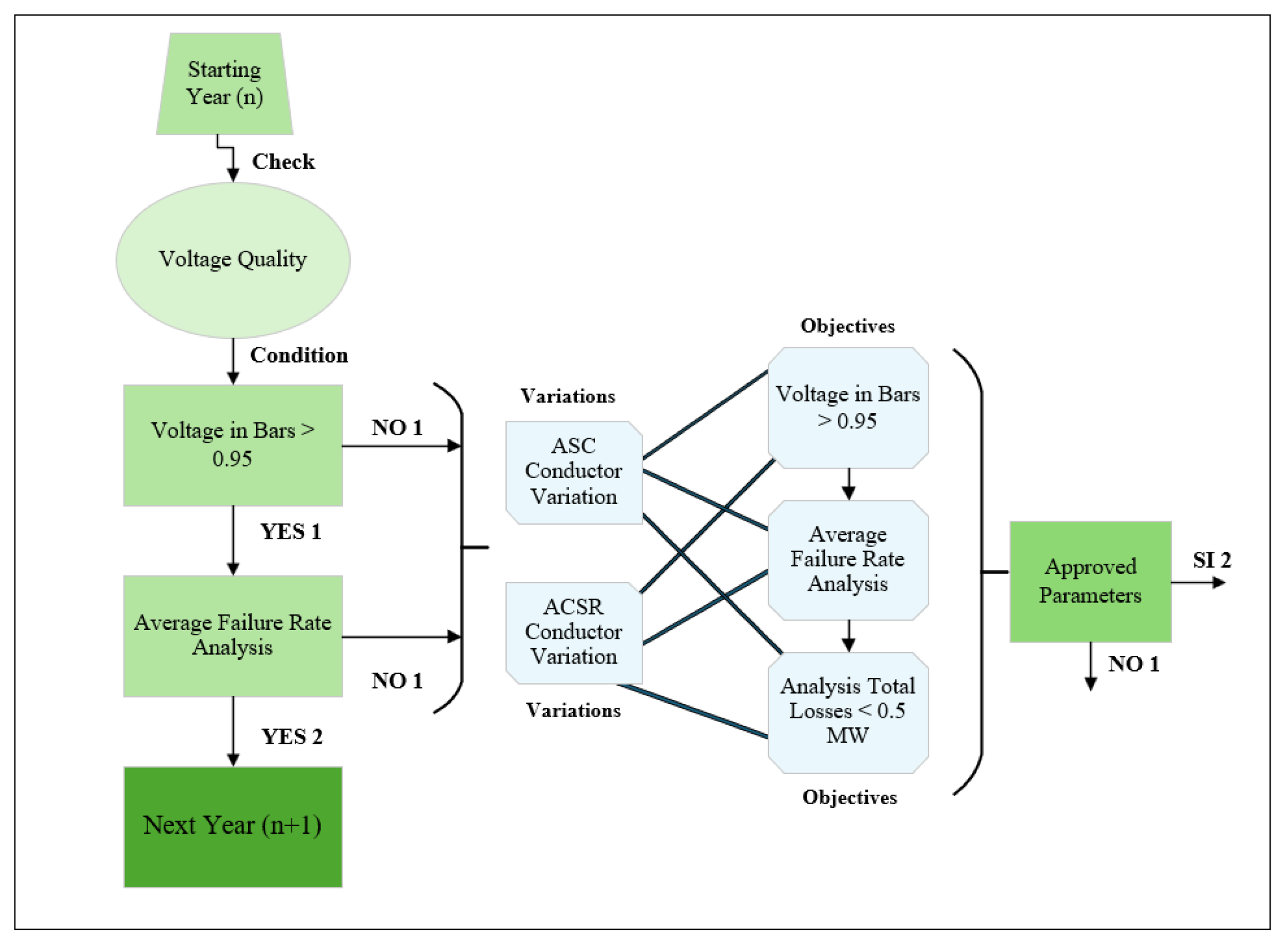
Figure 1 shows the decision-making flowchart used in the implementation of the multi-criteria function. The process begins by verifying voltage quality in each simulation year. If all bus voltages remain above the threshold of 0.95 p.u., the system advances to the next year without changes. Otherwise, an average failure rate (AFR) analysis is conducted. If the AFR exceeds the acceptable limit, various conductor types (ASC or ACSR) are evaluated as potential replacements. The objective is to achieve three performance criteria simultaneously: bus voltages above 0.95 p.u., AFR values within limits, and total system losses below 0.5 MW. When all objectives are satisfied, the solution is approved and used to update the system configuration for subsequent years.

The weighting of the criteria in the multi-criteria optimization function can be determined in two ways. One option is a mathematical approach based on the CRITIC method, which assigns weights to each criterion $W_i$ using the standard deviation of its data and its correlation with the other criteria. The weighting formula is defined as

$$W_i=S_i\sum (1-r_{ij})$$

(5)

where

• $W_i$: weight of criterion i.
• $S_i$: standard deviation of the data for criterion i.
• $r_{ij}$: correlation coefficient between criterion i and criterion j.

This method ensures that weights reflect both the variability and conflict between the criteria, allowing for a more objective balance in decision making.

Alternatively, the algorithm also provides the option for manual weight assignment based on human intervention. In such cases, the planner or utility can define the relative importance of each variable according to specific operational, regulatory, or economic priorities. This dual-mode structure allows the methodology to be adapted to either data-driven decision-making or client-driven planning strategies.

3. Case Study: IEEE 15-Bus Distribution System

The IEEE 15-bus distribution system was selected as it is widely used to represent compact urban distribution networks with relatively short radial feeders and moderate load diversity. Its structure allows for the clear identification of voltage drops and reliability issues in densely populated areas.

The continuous growth in demand causes instability in distribution systems due to their direct connection with end users. Traditional methods propose improving the system quality and stability, often through the use of reactive compensation, which is directly injected into the system. However, these approaches tend to overlook the behavior and impact of increasing the demand on the components of the distribution network.

Based on the above, the IEEE 15-bus distribution system template developed by Das D., Kothari D. P., and Kalam A. in 1995 was used. This system offers a simple and effective method for solving radial distribution networks and operates with a base voltage of 13.3 kV.

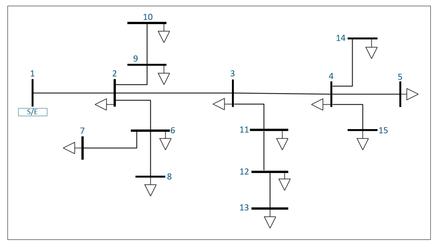
The following analysis presents a 5% annual demand increase over a 10-year period for the IEEE 15-bus distribution system. The configuration of this radial distribution network is shown in Figure 2.

Figure 2 shows the single-line diagram of the system. Bus 1 corresponds to the substation or source node (S/E), which supplies the entire network. Buses 2 to 15 represent load nodes connected through distribution lines. The downward-pointing arrows denote electrical loads at each bus. This radial topology is representative of typical medium-voltage distribution networks and is used for evaluating power flow, voltage profile, and reliability criteria.

To evaluate the long-term impact of demand growth, a 10-year simulation was performed with a 5% annual increase in electrical demand applied to each load node.

Table 3. Active power growth (MW) in the 15-bus distribution system.

Load	Year 0	Year 1	Year 3	Year 5	Year 7	Year 9	Year 10
Load 1	0	0	0	0	0	0	0
Load 2	44.1	46.305	51.051	56.284	62.053	68.414	71.834
Load 3	70	73.5	81.034	89.34	98.497	108.593	114.023
Load 4	140	147	162.068	178.679	196.994	217.186	228.045
Load 5	44.1	46.305	51.051	56.284	62.053	68.414	71.834
Load 6	140	147	162.068	178.679	196.994	217.186	228.045
Load 7	140	147	162.068	178.679	196.994	217.186	228.045
Load 8	70	73.5	81.034	89.34	98.497	108.593	114.023
Load 9	70	73.5	81.034	89.34	98.497	108.593	114.023
Load 10	44.1	46.305	51.051	56.284	62.053	68.414	71.834
Load 11	140	147	162.068	178.679	196.994	217.186	228.045
Load 12	70	73.5	81.034	89.34	98.497	108.593	114.023
Load 13	44.1	46.305	51.051	56.284	62.053	68.414	71.834
Load 14	70	73.5	81.034	89.34	98.497	108.593	114.023
Load 15	140	147	162.068	178.679	196.994	217.186	228.045

and

Table 4. Reactive power growth (MVAr) in the 15-bus distribution system.

Load	Year 0	Year 1	Year 3	Year 5	Year 7	Year 9	Year 10
Load 1	0	0	0	0	0	0	0
Load 2	44.991	47.24055	52.083	57.421	63.307	69.796	73.286
Load 3	71.4143	74.985015	82.671	91.145	100.487	110.787	116.326
Load 4	142.8286	149.97003	165.342	182.29	200.974	221.574	232.653
Load 5	44.991	47.24055	52.083	57.421	63.307	69.796	73.286
Load 6	142.8286	149.97003	165.342	182.29	200.974	221.574	232.653
Load 7	142.8286	149.97003	165.342	182.29	200.974	221.574	232.653
Load 8	71.4143	74.985015	82.671	91.145	100.487	110.787	116.326
Load 9	71.4143	74.985015	82.671	91.145	100.487	110.787	116.326
Load 10	44.991	47.24055	52.083	57.421	63.307	69.796	73.286
Load 11	142.8286	149.97003	165.342	182.29	200.974	221.574	232.653
Load 12	71.4143	74.985015	82.671	91.145	100.487	110.787	116.326
Load 13	44.991	47.24055	52.083	57.421	63.307	69.796	73.286
Load 14	71.4143	74.985015	82.671	91.145	100.487	110.787	116.326
Load 15	142.8286	149.97003	165.342	182.29	200.974	221.574	232.653

show the projected active and reactive power growth, respectively, at each load point of the IEEE 15-bus distribution system. These projections are essential for assessing system performance under future loading scenarios and for planning infrastructure reinforcements.

4. Results for the 15-Bus Distribution System

The implementation of traditional methods to mitigate the negative impacts caused by demand growth aims to improve the system’s power quality and reliability. However, these methods are often not aligned with the economic impact they entail during implementation. One of the main electrical components affected by increasing demand is the distribution line conductor. Due to its exposure to open air and environmental conditions, it is prone to corrosion or oxidation, which increases the resistance to current flow and leads to greater power losses in the system.

Based on the above, and in order to provide a feasible solution to growing demand, modifications to the conductors in the distribution system were carried out to evaluate their performance under voltage quality, loss reduction, and reliability improvement parameters—without resorting to traditional solutions such as capacitor banks, distributed generation, circuit duplication, or any other major system changes.

With the implementation of the multi-criteria function, which includes specific characteristics and constraints, the goal was to offer a technically and economically sustainable solution while maintaining or improving the system reliability and power quality. The most relevant modifications applied to the evaluated distribution systems are presented below.

4.1. Initial Conditions (Case 0)

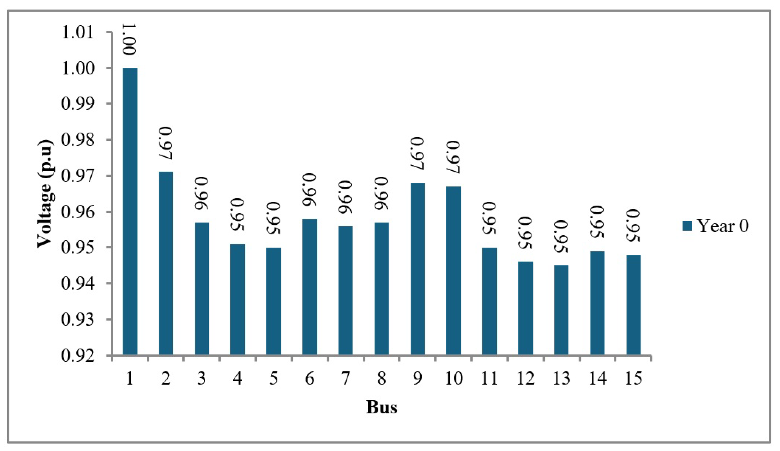
Prior to the development of the multi-criteria function, system parameters under initial conditions were obtained for each distribution model. These included the bus voltage in per unit (p.u.), total system losses in megawatts (MW), and the average failure rate of the conductors. The IEEE 15-bus distribution system showed voltages below the minimum threshold (0.95 p.u.) at buses 12, 13, 14, and 15, making it necessary to apply changes from year zero, as illustrated in Figure 3.

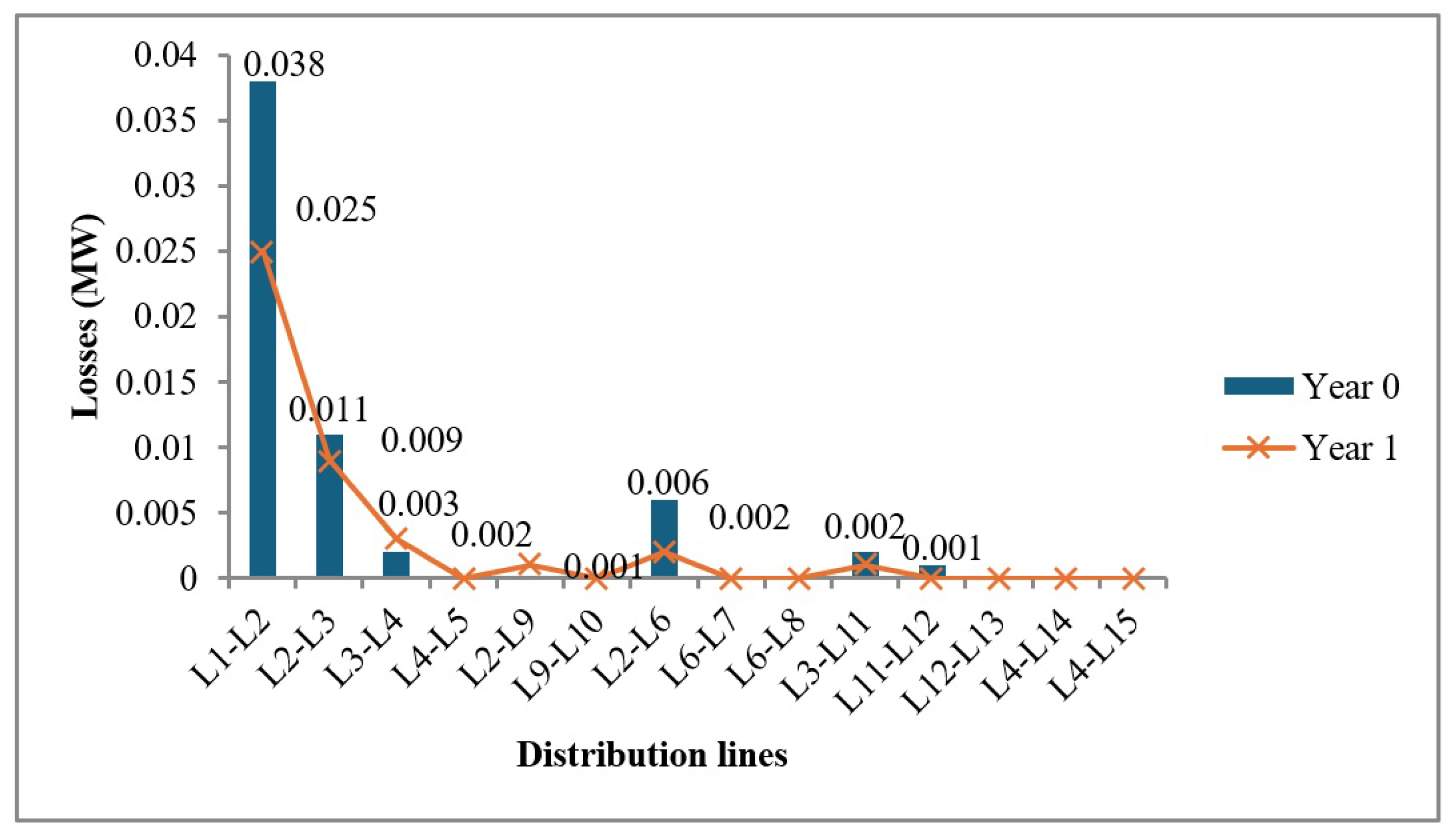
Based on the system loss analysis, the IEEE 15-bus model exhibited a total of 0.06 MW in losses. Notably, the most significant losses occurred in the following lines.

Regarding system losses, the IEEE 15-bus model exhibited a total power loss of 0.06 MW under initial conditions (year 0).

Table 5. Losses in the IEEE 15-bus model, year 0.

Line	Value	Unit
L1–L2	0.038	MW
L2–L3	0.011	MW
L3–L4	0.002	MW
L2–L6	0.006	MW
L3–L11	0.002	MW

details the most critical lines contributing to these losses. These values were obtained through power flow simulations and highlight the need to improve conductor efficiency, especially in the upstream segments of the distribution network.

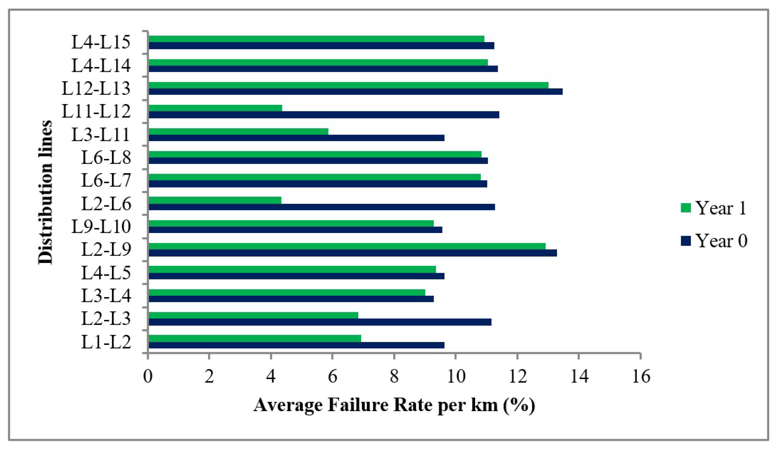
To evaluate the system’s reliability, the average failure rate per kilometer of the conductors was assessed. The IEEE 15-bus model showed a failure rate range between 9.56% (minimum) and 13.46% (maximum), particularly in lines L9–L10 and L12–L3.

4.2. Analysis of the 15-Bus Distribution System

Considering the voltage quality and system reliability as essential requirements for the distribution system, the multi-criteria function analysis was initiated in year 0. This was because the IEEE 15-bus model exhibited voltages below the minimum permissible threshold (0.95 p.u.), with a base voltage of 13.3 kV.

By applying the multi-criteria function, the conductors in lines L1–L2, L2–L3, L3–L4, L2–L6, L3–L11, and L11–L12 were replaced with the “Iris” type conductor from the ASC or AAC catalog, which has the following characteristics:

• Gauge: 2 AWG.
• Cross-sectional area: 33.62 mm².
• Resistance: 0.856 Ohm/km.
• Cost: 0.926 USD/m.

Replacing the conductors in the aforementioned lines improved the voltage profile of the system, reduced the total power losses, and decreased the average failure rate within the system.

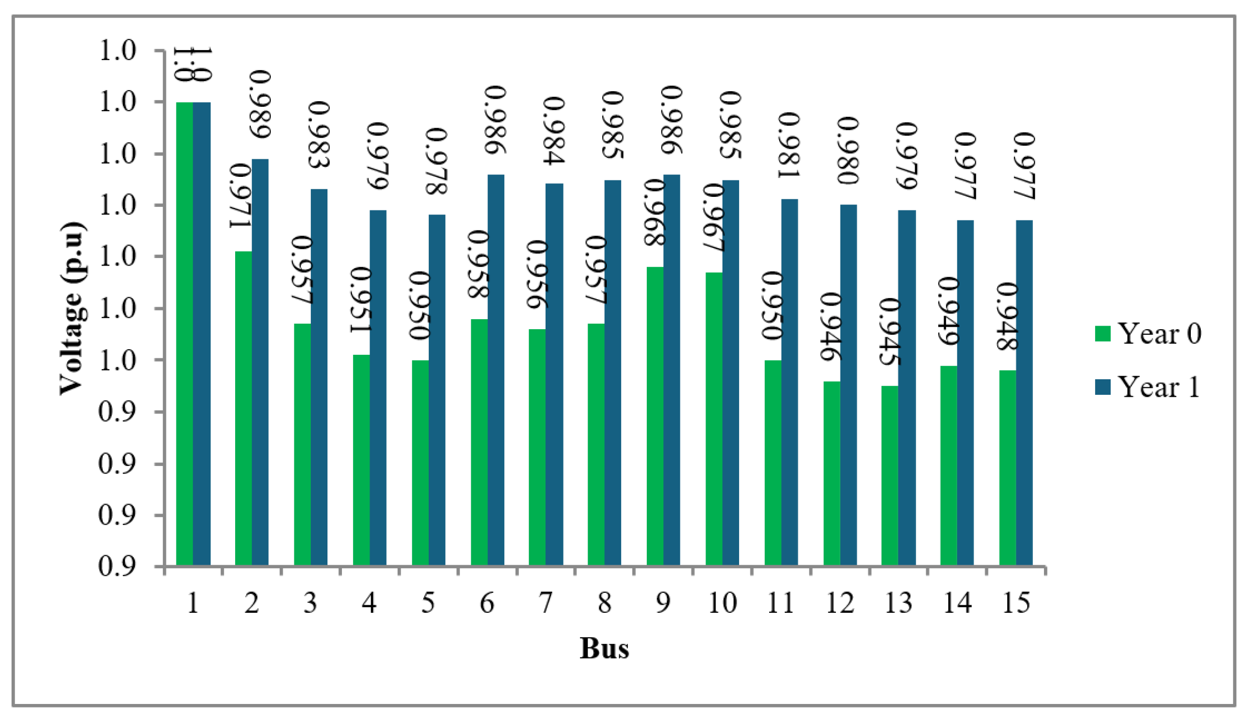
Figure 4 illustrates the voltage profile comparison between the system’s initial state (year 0) and the condition after replacing key distribution lines with higher-capacity conductors. The conductors were upgraded in lines L1–L2, L2–L3, L3–L4, L2–L6, L3–L11, and L11–L12. The implementation of these upgrades resulted in a significant voltage improvement, particularly at downstream buses where the voltage was originally below the minimum acceptable threshold of 0.95 p.u. The enhanced conductor specifications reduced voltage drops across the network, improving system performance under growing load conditions.

After replacing the conductors in distribution lines L1–L2, L2–L3, L3–L4, L2–L6, L3–L11, and L11–L12, the total system losses were reduced to 0.041 MW, and the partial resistances of the replaced lines significantly decreased.

The voltage improvement observed between year 0 and year 1, as shown in Figure 4, is directly attributed to the upgraded conductor specifications. The new “Iris” conductors feature a lower resistance and a larger cross-sectional area compared with the original lines, which substantially mitigates voltage drops under load conditions. This effect was most notable at the downstream buses, where voltage levels initially fell below the minimum threshold. Following the upgrades, all bus voltages remained above 0.95 p.u., which resulted in an overall improvement in the voltage stability across the system.

Figure 5 shows the comparison of active power losses across individual distribution lines in the IEEE 15-bus system before and after conductor replacements. In the initial state (Case 0), the most critical losses were concentrated in lines L1–L2 (0.038 MW), L2–L3 (0.025 MW), and L2–L6 (0.006 MW). After upgrading selected lines with conductors of lower resistance and a larger cross-sectional area, the losses in these segments dropped dramatically, almost to zero in most cases. This clearly demonstrates the effectiveness of the conductor replacements in minimizing resistive losses and improving the system’s overall energy efficiency.

Similarly, replacing the conductors also resulted in a reduction in the average failure rate throughout the system, as shown in Figure 6.

With the gradual 5% increase in load, no conductor replacements were required in the five years following the initial changes, as the system continued to meet the minimum voltage requirement (0.95 p.u.). It was observed that the next adjustment or conductor replacement should be carried out in year 6. The optimal solution in this case was the replacement of the conductor in distribution line L1–L2 with an ACSR-type conductor, which was characterized by the following:

• Gauge: 1/0 AWG.
• Cross-sectional area: 53.49 mm².
• Resistance: 0.5227 ohm/km.
• Cost: 1.24 USD/m.

After performing this replacement and applying the projected load growth for the following four years, it was determined that no further conductor replacements were necessary in the distribution system for any year beyond year 6. The voltage behavior over the final four years is shown in Figure 7.

The following expansion plan summarizes the adjustments made in year 0, including the changes applied to the distribution lines and their direct impacts on the system power quality and reliability.

The adjustments made in year 0, particularly the replacement of conductors in key lines, produced notable improvements in both the reliability and voltage quality. The V (p.u.) values reported in

Table 6. Expansion plan for year 0–year 1.

	Reliability Year 0		Reliability Year 1		Quality Year 0 and Year 1
Line	Conductor	AFR (%)	Conductor	AFR (%)	Bus	V (p.u.)	V (p.u.)
L1–L2	Alton 48.69	9.622	Iris	6.932	Bus 1	1.00	1.00
L2–L3	Swan	11.148	Iris	6.828	Bus 2	0.971	0.989
L3–L4	Sparrow	9.276	Iris	9.011	Bus 3	0.957	0.983
L4–L5	Akron 4	9.626	Akron 4	9.350	Bus 4	0.951	0.979
L2–L9	Turkey	13.283	Turkey	12.905	Bus 5	0.950	0.978
L9–L10	Akron 4	9.566	Akron 4	9.293	Bus 6	0.958	0.986
L2–L6	Akron 6	11.270	Iris	4.331	Bus 7	0.956	0.984
L6–L7	Swan	11.022	Swan	10.820	Bus 8	0.957	0.985
L6–L8	Swan	11.033	Swan	10.831	Bus 9	0.968	0.986
L3–L11	Akron	9.636	Iris	5.864	Bus 10	0.967	0.985
L11–L12	Akron	11.401	Iris	4.354	Bus 11	0.950	0.981
L12–L13	Turkey	13.465	Turkey	12.998	Bus 12	0.946	0.980
L4–L14	Akron 6	11.365	Akron 6	11.040	Bus 13	0.945	0.979
L4–L15	Swan	11.254	Swan	10.921	Bus 14	0.949	0.977
–	–	–	–	–	Bus 15	0.948	0.977

were justified by the electrical characteristics of the new conductors, including a reduced resistance and increased cross-sectional area. These characteristics significantly minimized the voltage drops along the upgraded lines, especially in downstream buses, ensuring that all voltages remained above the 0.95 p.u. threshold. The simulation results confirmed the stability of the system under projected growth, with no further reinforcement required until year 6.

In year 6, a second set of reinforcements was triggered as the cumulative demand growth began to slightly affect the voltage quality and reliability.

Table 7. Expansion plan for year 6–year 7.

	Reliability Year 6		Reliability Year 7		Quality Year 6 and Year 7
Line	Conductor	AFR (%)	Conductor	AFR (%)	Bus	V (p.u.)	V (p.u.)
L1–L2	Iris	8.032	Raven	7.642	Bus 1	1.00	1.00
L2–L3	Iris	7.920	Iris	7.530	Bus 2	0.986	0.990
L3–L4	Iris	10.452	Iris	10.062	Bus 3	0.978	0.982
L4–L5	Akron 4	9.408	Akron 4	9.370	Bus 4	0.9740	0.977
L2–L9	Turkey	12.945	Turkey	12.905	Bus 5	0.972	0.976
L9–L10	Akron 4	9.331	Akron 4	9.303	Bus 6	0.983	0.986
L2–L6	Iris 6	5.0198	Iris	4.619	Bus 7	0.980	0.983
L6–L7	Swan	10.865	Swan	10.820	Bus 8	0.981	0.984
L6–L8	Swan	10.876	Swan	10.842	Bus 9	0.982	0.986
L3–L11	Iris	3.705	Raven	2.963	Bus 10	0.981	0.984
L11–L12	Iris	4.380	Iris	3.962	Bus 11	0.976	0.979
L12–L13	Turkey	13.078	Turkey	13.038	Bus 12	0.974	0.978
L4–L14	Akron 6	11.108	Akron 6	11.014	Bus 13	0.973	0.976
L4–L15	Swan	10.99	Swan	10.954	Bus 14	0.971	0.974
L9–L11	Akron	11.53	Iris	9.834	Bus 15	0.970	0.974

shows that the replacement of conductors, especially in lines L1–L2 (upgraded to Raven type) and L3–L11, resulted in further reductions in the average failure rates and voltage deviations. These targeted enhancements allowed the system to maintain operational performance within acceptable thresholds and avoided more aggressive or costly upgrades. The multi-criteria function effectively prioritized the most impactful replacements based on the evolving conditions of the network.

5. Case Study: 33-Bus Distribution System

The IEEE 33-bus distribution system was selected because it is commonly used to simulate rural or suburban networks characterized by long feeder lengths and dispersed loads. This model is particularly useful for analyzing voltage regulation and conductor performance over extended distances.

The 33-bus distribution system, developed by Kashem M. A., Ganapathy V., Jasmon G. B., and Buhari M. in the year 2000, presents a method for minimizing losses in distribution networks. This system operates with a base voltage of 12.66 kV.

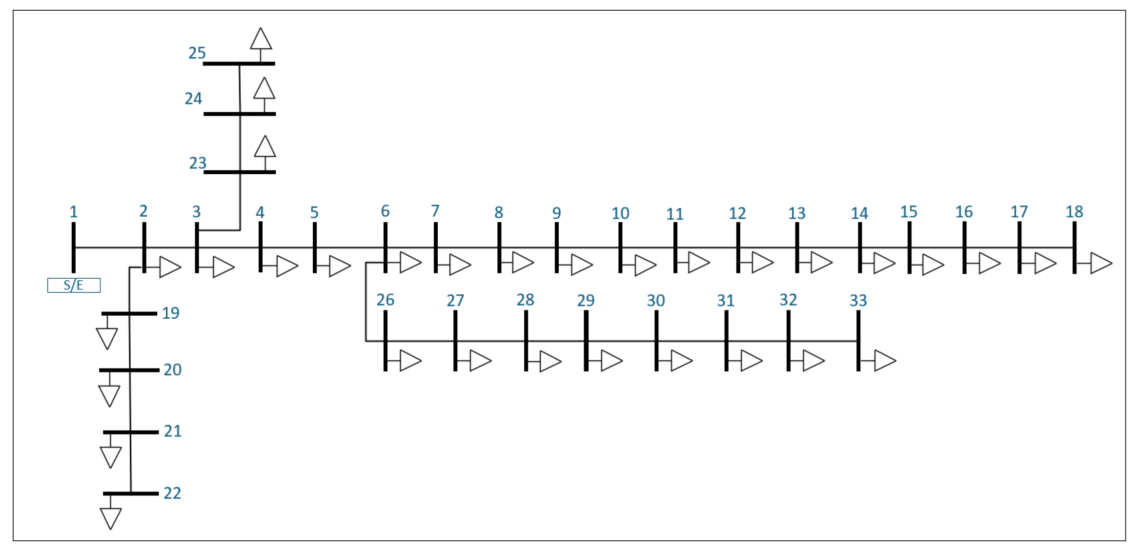
Figure 8 shows the single-line diagram of the IEEE 33-bus distribution system, which is widely used for testing optimization and loss minimization strategies in distribution networks. Bus 1 corresponds to the main substation (S/E), which supplies the entire system. Buses 2 to 33 represent load points, each associated with a distributed electrical demand. The network features a radial structure with long feeders and lateral branches, making it ideal for analyzing performance under rural or suburban operating conditions. This configuration supports detailed studies on voltage drops, conductor performance, and reliability along extended paths.

To evaluate the long-term performance of the IEEE 33-bus distribution system under load growth, a 5% annual increase in demand was simulated over a 10-year horizon.

Table 8. Active power growth (MW) in the 33-bus distribution system.

Load	Year 0	Year 1	Year 3	Year 5	Year 7	Year 9	Year 10
Load 1	0	0	0	0	0	0	0
Load 2	100	105	115.76	127.63	140.71	155.13	162.89
Load 3	90	94.5	104.19	114.87	126.64	139.62	146.6
Load 4	120	126	138.92	153.15	168.85	186.16	195.47
Load 5	60	63	69.46	76.58	84.43	93.08	97.73
Load 6	60	63	69.46	76.58	84.43	93.08	97.73
Load 7	200	210	231.53	255.26	281.42	310.27	325.78
Load 8	200	210	231.53	255.26	281.42	310.27	325.78
Load 9	60	63	69.46	76.58	84.43	93.08	97.73
Load 10	60	63	69.46	76.58	84.43	93.08	97.73
Load 11	45	47.25	52.09	57.43	63.32	69.81	73.3
Load 12	60	63	69.46	76.58	84.43	93.08	97.73
Load 13	60	63	69.46	76.58	84.43	93.08	97.73
Load 14	120	126	138.92	153.15	168.85	186.16	195.47
Load 15	60	63	69.46	76.58	84.43	93.08	97.73
Load 16	60	63	69.46	76.58	84.43	93.08	97.73
Load 17	60	63	69.46	76.58	84.43	93.08	97.73
Load 18	90	94.5	104.19	114.87	126.64	139.62	146.6
Load 19	90	94.5	104.19	114.87	126.64	139.62	146.6
Load 20	90	94.5	104.19	114.87	126.64	139.62	146.6
Load 21	90	94.5	104.19	114.87	126.64	139.62	146.6
Load 22	90	94.5	104.19	114.87	126.64	139.62	146.6
Load 23	90	94.5	104.19	114.87	126.64	139.62	146.6
Load 24	420	441	486.2	536.04	590.98	651.56	684.14
Load 25	420	441	486.2	536.04	590.98	651.56	684.14
Load 26	60	63	69.46	76.58	84.43	93.08	97.73
Load 27	60	63	69.46	76.58	84.43	93.08	97.73
Load 28	60	63	69.46	76.58	84.43	93.08	97.73
Load 29	120	126	138.92	153.15	168.85	186.16	195.47
Load 30	200	210	231.53	255.26	281.42	310.27	325.78
Load 31	150	157.5	173.64	191.44	211.07	232.7	244.33
Load 32	210	220.5	243.1	268.02	295.49	325.78	342.07
Load 33	60	63	69.46	76.58	84.43	93.08	97.73

presents the projected active power demand at each load bus for selected years. These projections were used to assess the need for reinforcements, such as conductor replacements, and to evaluate their impact on voltage quality, power losses, and system reliability.

The objective was to generate various case studies based on the IEEE 33-bus distribution system by identifying the specific data of the electrical components. Then, using the multi-criteria function, the optimal results were obtained by considering key parameters, such as resistance, power losses, economic impact, voltage deviation, and average failure rate.

In parallel with the active power growth, the reactive power demand in the IEEE 33-bus distribution system was also projected with a 5% annual increase over a 10-year period.

Table 9. Reactive power growth (MVAr) in the 33-bus distribution system.

Load	Year 0	Year 1	Year 3	Year 5	Year 7	Year 9	Year 10
Load 1	0	0	0	0	0	0	0
Load 2	60	63	69.46	76.58	84.43	93.08	97.73
Load 3	40	42	46.31	51.05	56.28	62.05	65.16
Load 4	80	84	92.61	102.1	112.57	124.11	130.31
Load 5	30	31.5	34.73	38.29	42.21	46.54	48.87
Load 6	20	21	23.15	25.53	28.14	31.03	32.58
Load 7	100	105	115.76	127.63	140.71	155.13	162.89
Load 8	100	105	115.76	127.63	140.71	155.13	162.89
Load 9	20	21	23.15	25.53	28.14	31.03	32.58
Load 10	20	21	23.15	25.53	28.14	31.03	32.58
Load 11	30	31.5	34.73	38.29	42.21	46.54	48.87
Load 12	35	36.75	40.52	44.67	49.25	54.3	57.01
Load 13	35	36.75	40.52	44.67	49.25	54.3	57.01
Load 14	80	84	92.61	102.1	112.57	124.11	130.31
Load 15	10	10.5	11.58	12.76	14.07	15.51	16.29
Load 16	20	21	23.15	25.53	28.14	31.03	32.58
Load 17	20	21	23.15	25.53	28.14	31.03	32.58
Load 18	40	42	46.31	51.05	56.28	62.05	65.16
Load 19	40	42	46.31	51.05	56.28	62.05	65.16
Load 20	40	42	46.31	51.05	56.28	62.05	65.16
Load 21	40	42	46.31	51.05	56.28	62.05	65.16
Load 22	40	42	46.31	51.05	56.28	62.05	65.16
Load 23	50	52.5	57.88	63.81	70.36	77.57	81.44
Load 24	200	210	231.53	255.26	281.42	310.27	325.78
Load 25	200	210	231.53	255.26	281.42	310.27	325.78
Load 26	25	26.25	28.94	31.91	35.18	38.78	40.72
Load 27	25	26.25	28.94	31.91	35.18	38.78	40.72
Load 28	20	21	23.15	25.53	28.14	31.03	32.58
Load 29	70	73.5	81.03	89.34	98.5	108.59	114.02
Load 30	600	630	694.58	765.77	844.26	930.8	977.34
Load 31	70	73.5	81.03	89.34	98.5	108.59	114.02
Load 32	100	105	115.76	127.63	140.71	155.13	162.89
Load 33	40	42	46.31	51.05	56.28	62.05	65.16

summarizes the evolution of reactive power demand at each load bus for selected years. These values are critical for assessing voltage regulation requirements and the potential need for compensation devices or conductor upgrades to maintain acceptable voltage profiles across the system.

6. Results for the 33-Bus Distribution System

The analysis of the multi-criteria function depends on the input data and existing constraints in the distribution system. Therefore, an initial analysis of the IEEE 33-bus system was conducted to assess its behavior throughout the demand growth period.

6.1. Initial Conditions (Case 0)

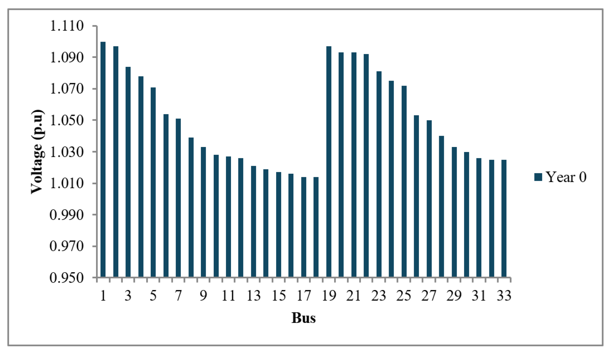
Since the IEEE 33-bus distribution system did not exhibit voltages below the minimum threshold (0.95 p.u.), and the voltage quality parameter remains above the established minimum, it was not necessary to conduct a voltage quality analysis for year 0. The minimum voltage recorded was 1.014 p.u. at bus 18, as shown in Figure 9.

The IEEE 33-bus model satisfied the voltage quality requirements for year 0, and the total power losses (0.168 MW) remained below the expected limits. Thus, a full loss analysis was not required for this year. However, the most significant losses are presented in the

Table 10. Losses in the IEEE 33-bus model, year 0.

Line	Value	Unit
L2–L3	0.038	MW
L5–L6	0.011	MW
L4–L5	0.002	MW
L3–L4	0.006	MW

.

To assess the system’s reliability conditions, the average failure rate per kilometer was evaluated. The IEEE 33-bus model showed a range between 5.62% (minimum) and 14.29% (maximum), with the most affected lines being L1–L2 and L21–L8.

6.2. Analysis of the 33-Bus Distribution System

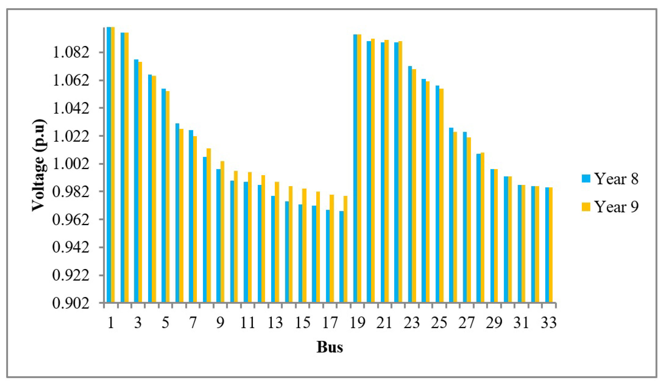
Since the IEEE 33-bus distribution system maintained voltage levels above the minimum threshold (0.95 p.u.) in year 0, a 5% increase in load was applied each year. As the years progressed, the voltage did not fall below the minimum threshold, thus the voltage quality remained compliant. Therefore, the system losses were analyzed instead, and in year 8, conductor replacements were deemed necessary in the following lines: L7–L8, L9–L10, L12–L13, L16–L17, L19–L20, and L27–L28. These lines were replaced with the following ASC or AAC-type conductor:

• Gauge: 2 AWG.
• Cross-sectional area: 33.62 mm².
• Resistance: 0.856 Ohm/km.
• Cost: 0.926 USD/m.

The replacement of the abovementioned conductors in the specified distribution lines led to an improvement in the voltage profiles at buses 10, 11, 12, 13, 14, 15, 16, 17, 18, 20, 21, and 22, as illustrated in Figure 10.

The total power losses in the IEEE 33-bus distribution system in year 8 reached 0.411 MW. After the conductor replacements in the specified lines, the total losses in year 9 decreased to 0.394 MW. Likewise, the maximum average failure rate per kilometer in year 8 was 11.21% in the previously mentioned lines. In year 9, after replacing the conductors, this value was reduced to 7.05%.

The following table presents the expansion plan reflecting the most relevant changes implemented in year 8. It highlights the improvements in power quality and system reliability that resulted from the conductor replacements.

After several years of load growth, the IEEE 33-bus system began to show early signs of voltage deviation and increased failure risk in specific segments. Consequently, targeted conductor replacements were implemented in year 8.

Table 11. Expansion plan for year 8–year 9.

	Reliability Year 8		Reliability Year 9		Quality Year 8 and Year 9
Line	Conductor	AFR (%)	Conductor	AFR (%)	Bus	V (p.u.)	V (p.u.)
L7–L8	Swan	11.968	Iris	7.529	Bus 8	1.007	1.013
L9–L10	Swan	12.304	Iris	7.740	Bus 9	0.998	1.004
L12–L13	Swan	12.441	Iris	7.826	Bus 12	0.997	0.994
L16–L17	Swan	12.633	Iris	7.947	Bus 13	0.979	0.989
L19–L20	Swan	11.214	Iris	7.054	Bus 14	0.975	0.986
L27–L28	Swan	11.980	Iris	7.536	Bus 15	0.973	0.984
L18–L19	Swan	11.871	Iris	7.413	Bus 16	0.972	0.982
L15–L17	Swan	12.135	Iris	7.315	Bus 17	0.969	0.980

presents the expansion plan comparing reliability (average failure rate, AFR) and voltage quality indicators (V in p.u.) before and after these upgrades. The results confirm that replacing lines such as L7–L8, L9–L10, L12–L13, and L27–L28 with higher-performance conductors significantly improved both operational reliability and voltage profiles by year 9.

7. Discussion

The continuous growth in energy demand generates significant stress on distribution systems, directly affecting the quality and reliability of the electrical service provided to end users. In response, electrical engineers typically propose various conventional solutions, such as the injection of reactive components, the incorporation of distributed generation, or the upgrade of existing infrastructure. However, these approaches, while technically effective, often fail to account for their economic implications, resulting in a considerable financial burden that is ultimately transferred to consumers.

Given this situation, it becomes essential to explore alternative strategies that can mitigate the impact of demand growth while minimizing investment costs without compromising the system performance in terms of power quality and reliability. The development and application of a multi-criteria decision-making (MCDM) approach allows for the integration of multiple technical and economic variables and constraints into a single optimization framework. By accurately defining input parameters and restrictions, the MCDM method yields optimal solutions tailored to the evolution of the demand, enabling decision-making that is both technically viable and economically sustainable. This approach offers a promising alternative to traditional methods, as it balances performance enhancement with cost-effectiveness in the management of distribution networks.

Several recent studies addressed distribution system reinforcement under demand growth, often focusing on optimal reinforcement timing and associated cost savings. For instance, recent studies proposed a reinforcement strategy based on load thresholds, while alternative approaches rely on cost–benefit analysis to determine the optimal year for conductor replacement. Compared with these approaches, our method offers a more holistic perspective by integrating multiple criteria—voltage quality, failure rate, and economic cost—into a single optimization framework. Notably, our results indicate that a single reinforcement action in year 0 can ensure stable operation for up to five years in the IEEE 15-bus case, thereby postponing additional investments. This contrasts with strategies requiring more frequent interventions, and highlights the economic efficiency of multi-criteria analysis when applied to distribution system planning.

8. Conclusions

The planning of distribution system expansion with a focus on voltage quality and reliability is crucial for ensuring long-term efficiency, resilience, and service continuity. Integrating these criteria into system design and decision-making processes enables a more adaptive and robust energy infrastructure—one capable of meeting increasing demand while minimizing losses, maintaining voltage stability, and optimizing resource utilization. This comprehensive approach, supported by advanced modeling techniques and effective system management, is vital to addressing future energy challenges and improving end-user satisfaction.

In this study, two standardized IEEE distribution models—15-bus and 33-bus systems—were analyzed using load flow simulations to extract key electrical parameters, including bus voltages, associated loads, line resistances, and base voltage levels (13.3 kV and 12.66 kV, respectively). These parameters facilitated the calculation of the current through each line and the estimation of the average failure rate per kilometer, a critical reliability indicator.

To simulate real-world scenarios, a projected annual demand growth of 5% was applied to both systems over a 10-year horizon. As expected, the results revealed a progressive degradation of voltage quality, an increase in system losses, and a decline in overall reliability as demand increased. These trends highlighted the need for strategic system upgrades and enabled the definition of a structured optimization strategy through multi-criteria analysis.

For the IEEE 15-bus system, the demand growth necessitated early action. In year 0, conductor replacements were applied to lines L1–L2, L2–L3, L3–L4, L2–L6, L3–L11, and L11–L12 using a type “Iris” conductor. This intervention significantly improved the voltage profile, reduced the power losses, and decreased the failure rates. For instance, the voltages at buses 3, 4, 5, 12, 13, 14, and 15 improved from initial values of 0.957, 0.951, 0.950, 0.946, 0.945, 0.949, and 0.948 p.u. to 0.983, 0.979, 0.978, 0.980, 0.979, 0.977, and 0.977 p.u., respectively. Likewise, the losses in key lines, such as L1–L2 and L2–L3, decreased from 0.038 MW and 0.011 MW to 0.025 MW and 0.009 MW, respectively. The average failure rates in the same lines also declined, for example, L1–L2 from 9.622% to 6.932% and L3–L11 from 9.636% to 5.864%.

For the 33-bus system, the MCDM analysis revealed that no immediate action was required during the early years, as the voltage levels and system losses remained within acceptable limits. However, by year 8, an increase in the total losses to 0.411 MW and high failure rates in certain lines prompted a targeted expansion plan. Conductor replacements were carried out in lines L7–L8, L9–L10, L12–L13, L16–L17, L19–L20, and L27–L28. These actions resulted in voltage improvements at buses 13–17 from the initial values of 0.979, 0.975, 0.973, 0.972, and 0.969 p.u. to 0.989, 0.986, 0.984, 0.982, and 0.980 p.u., respectively. Additionally, the average failure rates in the affected lines were reduced significantly, e.g., L9–L10 from 12.304% to 7.740%, and L19–L20 from 11.214% to 7.054%.

In summary, the application of a multi-criteria optimization strategy allowed for cost-effective and technically sound decisions regarding system reinforcement. The case studies demonstrated the feasibility of improving the distribution system performance by optimizing the conductor selection and timing of upgrades, ultimately ensuring the maintenance of power quality and system reliability under increasing demand scenarios.

While the proposed method shows promising results, it is important to acknowledge certain limitations of this study. The analysis assumed a constant 5% annual load growth, which may not reflect the real-world variability influenced by seasonality, economic shifts, or the integration of new technologies. Furthermore, the current model does not include distributed energy resources, such as photovoltaic systems or energy storage, which could significantly affect the system performance and planning decisions. Future research should focus on extending the methodology to include dynamic load models, probabilistic load forecasting, and the integration of renewable energy sources. Additionally, incorporating stochastic variables and sensitivity analyses could enhance the robustness of the multi-criteria decision framework under uncertain conditions.