Two-Stage Dynamic Partitioning Strategy Based on Grid Structure Feature and Node Voltage Characteristics for Power Systems

Abstract

To enhance the adaptability of grid partitioning under transient scenarios, this paper proposes a two-stage dynamic partitioning strategy based on structure–function coupling. Electrical coupling strength is first characterized using short-circuit impedance and the sensitivity between reactive power and voltage, while transient voltage correlation is incorporated through cosine similarity as edge weights in a graph model. Grid partitioning is then conducted by maximizing modularity through a staged approach that ensures network connectivity and automatically determines partition numbers. Case studies on the modified IEEE 39-bus system demonstrate that compared with transient voltage-based partitioning and conventional complex network methods, the proposed approach improves modularity by 69%, reduces the maximum post-fault voltage deviation by 38.6%, and achieves the highest regional decoupling rate. The result shows strong intra-regional cohesion and weak inter-regional connectivity, verifying the strategy’s effectiveness in enhancing adaptability and decoupling under transient conditions.

1. Introduction

At present, power system voltage regulation primarily relies on automatic voltage control (AVC) systems, which aim to optimize and control steady-state voltage in a secure and economical manner. In the 20th century, Electricity Company of France pioneered a hierarchical and partitioned AVC system based on concepts such as “voltage control zones” and “central bus voltage”. A key aspect of this approach is the division of the grid into smaller subsystems characterized by strong intra-zone coupling and weak inter-zone coupling, enabling independent voltage regulation within each zone. This highlights that effective and rational grid partitioning is essential for implementing regional voltage control [1,2].

Against the backdrop of energy industry transformation, the construction of a new-type power system has become a key strategy for achieving the “dual-carbon” goals. Unlike conventional power systems dominated by synchronous generators, the increasing integration of renewable energy sources such as wind and solar introduces significant uncertainty, volatility, and intermittency into system operation. These characteristics pose new challenges to maintaining system stability and control. In this context, reactive power and voltage regulation play a critical role in ensuring the secure and economical operation of the power grid. Moreover, reasonable power system partitioning serves as a fundamental prerequisite for effective control, operation coordination, and resilience enhancement in large-scale interconnected networks.

Power grid partitioning is essentially a combinatorial optimization problem, involving the determination of both the number of regions (voltage control zones) and the assignment of nodes to these regions, with the objective of maximizing a given decoupling metric [3,4]. Two key challenges in this process are how to evaluate electrical coupling between nodes and how to determine the optimal number of partitions. Traditional partitioning approaches are often based on geographical boundaries, administrative divisions, or historical operating experience. However, such criteria fail to accurately reflect the actual operating conditions of the grid. To address this limitation, extensive research efforts have been undertaken both domestically and internationally.

Currently, commonly used measures of electrical distance are primarily based on steady-state system information. Ref. [5] defines electrical distance using the reactive power–voltage sensitivity matrix derived from the Jacobian matrix of power flow equations and applies hierarchical clustering for grid partitioning. In Ref. [6], electrical distance is represented by assigning weights to transmission lines based on their impedance, with the Dijkstra algorithm used for partitioning. Other studies incorporate local voltage stability indices to characterize electrical coupling. However, these approaches rely solely on steady-state data and do not account for transient dynamics following disturbances. As a result, such metrics may not be suitable for applications in transient voltage control and fall short in addressing emerging challenges in modern power systems. In contrast, recent efforts in transient-based grid partitioning have proposed alternative indicators, such as transient voltage sag area [7], voltage time-series trajectories [8], and node voltage fluctuations [9], to more accurately characterize electrical coupling under dynamic conditions.

From the perspective of optimization objectives, existing voltage partitioning methods can be broadly categorized into two types: clustering-based approaches and complex network theory-based approaches. Clustering-based methods: Ref. [10] transforms the partitioning problem into a hierarchical classification task, applying hierarchical clustering to divide the distribution network. Ref. [11] employs local expansion theory to group nodes from the bottom up until partitions are formed. Related studies have proposed methods based on spectral clustering, k-means, and recursive bisection [12,13,14]. These approaches typically require manual specification of the number of partitions, as the number of regions is not treated as a decision variable. Consequently, the resulting partition is optimal only with respect to the predefined number of zones. Complex network-based methods [15,16,17,18]: To address the limitations of clustering approaches, alternative methods based on complex network theory have been developed [19]. One such method constructs a graph model with edge weights defined by the actual reactive power flow along transmission lines, and performs partitioning by optimizing an improved modularity metric, allowing the optimal number of partitions to be determined automatically. Ref. [20] introduces a community detection algorithm based on local similarity, in which node similarity reflects topological proximity. Nodes with high mutual similarity are grouped into the same partition. However, this approach may assign nodes with high similarity but large electrical distance to the same partition, resulting in reduced partitioning effectiveness and increased challenges for voltage stability.

To address these challenges, this study introduces a partitioning approach based on complex network theory, incorporating electrical coupling strength and cosine similarity metrics. The method aims to achieve voltage control-oriented decoupling while maintaining robustness by accounting for both network topology and electrical connectivity. First, an electrical coupling strength index between reactive power source nodes and load nodes is constructed using the network admittance matrix. Based on this index, load nodes are aggregated around their corresponding source nodes to form the initial pre-partition. Next, a system-wide undirected weighted graph is established using node voltage correlation derived from transient voltage characteristics. Finally, network-wide clustering is performed by optimizing the modularity metric from community detection theory, resulting in the final partitioning scheme. The partitioning method proposed in this study takes into account both the structural characteristics and the electrical properties of the power network. In contrast to traditional approaches, it further incorporates the transient voltage behavior of nodes, enabling a more functionally coherent and dynamically responsive regional division.

2. The Complex Network Based on Structure–Function Coupling

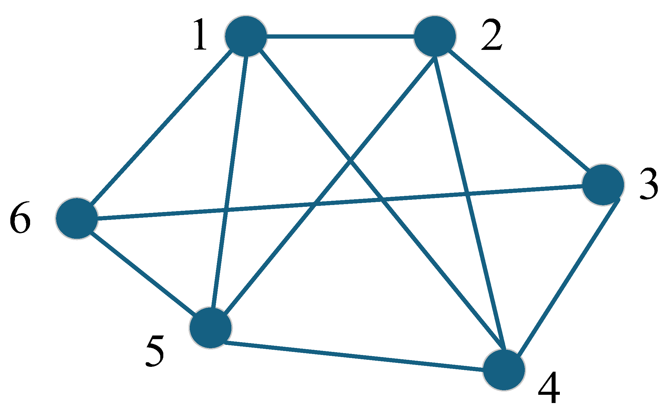
2.1. Complex Network Features of Electrical Grid

Complex networks serve as abstractions of complex systems, where nodes represent individual components and edges denote the relationships among them based on specific interaction rules. Various types of complex networks exist in the real world, including social networks, the internet, and power systems. As a theoretical framework, complex network theory investigates the statistical properties of network topologies to uncover universal principles governing diverse systems. Its central objective is to understand how structural features influence system functionality and dynamic behavior. In recent years, significant advances have been made in this field, revealing several key statistical characteristics of complex networks, such as small-world properties and community structures [21].

The small-world property refers to a network characteristic defined by a high clustering coefficient and a low average path length. It reflects a key structural feature of complex networks, where most nodes are not directly connected to each other, yet any node can be reached from another through only a few intermediate steps [22]. Watts formally characterized this phenomenon by identifying specific topological features that define the small-world property:

$$\left\{\begin{array}{c}C>>C_{\mathrm{random}}\\ L\ge L_{\mathrm{random}}\end{array}\right.$$

(1)

where C represents the clustering coefficient; and L represents the average path of the network.

As a typical example of an engineered complex network, the power grid exhibits topological evolution that inherently aligns with the small-world property. When applying complex network theory to characterize its topological structure, several commonly used parameters include (1) the adjacency matrix, (2) the shortest path length, (3) the node degree, and (4) the clustering coefficient.

Adjacency Matrix: This matrix describes the relationships between nodes in a system of N nodes, thereby encapsulating the most fundamental topological properties of the network. As illustrated in Figure 1, if a connection exists between two distinct nodes, the corresponding element in the adjacency matrix is set to 1; otherwise, it is 0. Accordingly, the adjacency matrix A = (a_ij)_N×N is defined as follows:

$$A=\left\{\begin{array}{l}{a}_{ij}=1,i\ne j\mathrm{and}\mathrm{directly}\mathrm{connected}\\ a_{ij}=0,\mathrm{others}\end{array}\right.$$

(2)

By definition, the adjacency matrix of the six-node system shown in Figure 1 is as follows:

$$A=\left[\begin{array}{cccccc}0& 1& 0& 1& 1& 1\\ 1& 0& 1& 1& 1& 0\\ 0& 1& 0& 1& 0& 1\\ 1& 1& 1& 0& 1& 0\\ 1& 1& 0& 1& 0& 1\\ 1& 0& 1& 0& 1& 0\end{array}\right]$$

Shortest Path: The distance between two nodes in a network is defined by the length of the shortest path connecting them, i.e., the minimum number of edges traversed between the two nodes. Based on this metric, other parameters, such as the average path length of the network, can also be derived.

Node Degree: As a key parameter in complex network theory, node degree reflects both the connectivity and influence of a node within the network. According to the adjacency matrix, the degree k_i of node i represents the number of connections it has to other nodes. Evidently, a higher degree indicates the greater importance of the node within the overall network. The degree is defined as follows:

$$k_i={\displaystyle \sum _{j=1}^n{a}_{ij}=}{\displaystyle \sum _{j=1}^n{a}_{ji}}$$

(3)

Clustering Coefficient: The clustering coefficient is an important metric used to quantify the degree of node aggregation in a network. It reflects how closely a node’s neighbors are interconnected. Specifically, the clustering coefficient of a node is defined as the ratio of the actual number of edges among its neighboring nodes to the maximum possible number of such edges. It is formally expressed as follows:

$$C={\displaystyle \frac{N_i}{k_i(k_i-1)/2}}$$

(4)

where N_i represents the number of actually connected edges to the neighboring nodes and k_i (k_i − 1)/2 represents the number of edges present in at most k_i neighboring nodes.

Another important feature of complex networks is community structures. As illustrated in Figure 2, studies have shown that nodes sharing similar properties tend to form densely connected groups, or communities, while connections between different communities are relatively sparse. This phenomenon characterizes the community structure of complex networks [23].

As a large-scale and complex system, the power grid often exhibits local aggregation effects due to the non-uniform distribution of connections among nodes. Specifically, the network can be divided into multiple subnetworks, where intra-subnetwork connections are relatively dense, while inter-subnetwork connections are sparse. This structural pattern aligns with the small-world property and community structure characteristics of complex network theory, making community-based approaches a suitable framework for analyzing power grid partitioning features.

2.2. Electrical Functional Features of Electrical Grid

2.2.1. Electrical Coupling Strength

In power systems, the electrical characteristics describing system operation encompass both steady and transient state. As a representative steady-state indicator, the sensitivity of reactive power and voltage effectively reflects the control capability of reactive power source nodes and load nodes. In this paper, reactive power source nodes refer to PV nodes capable of providing reactive power support, including synchronous generators, wind turbines, and photovoltaic (PV) units operating under the voltage control mode. For an N-node power system with N_S reactive power source nodes and N_L load nodes, the reactive power voltage power flow iteration can be expressed using the PQ decomposition method as BΔV = ΔQ. On this basis, the equation can be derived as follows:

$$\left[\begin{array}{c}\mathsf{\Delta }{\mathit{Q}}_L\\ \mathsf{\Delta }{\mathit{Q}}_S\end{array}\right]=\left[\begin{array}{cc}{\mathit{S}}_{LL}& {\mathit{S}}_{LS}\\ {\mathit{S}}_{SL}& {\mathit{S}}_{SS}\end{array}\right]\left[\begin{array}{c}\mathsf{\Delta }{\mathit{V}}_L\\ \mathsf{\Delta }{\mathit{V}}_S\end{array}\right]$$

(5)

Assuming the load node injected reactive power is unchanged, i.e., ΔQ_L = 0, the following can be obtained:

$$\mathsf{\Delta }{\mathit{V}}_L=-{\mathit{S}}_{LL}^{-1}{\mathit{S}}_{LS}\mathsf{\Delta }{\mathit{V}}_S$$

(6)

The formula ${\mathit{S}}_{LL}^{-1}{\mathit{S}}_{LS}$ is defined as the sensitivity matrix S, with a dimension of N_L × N_S, based on which the sensitivity of reactive power and voltage for reactive power source nodes to load nodes is expressed as follows:

$$\mathit{S}=\mathbf{\Delta }{\mathit{V}}_{\mathbf{L}}/\mathbf{\Delta }{\mathit{Q}}_{\mathbf{S}}$$

(7)

Not only does the short-circuit impedance, which is also a steady-state quantity, characterize the degree of electrical connection between the reactive source node and the load node, the short-circuit impedance distance obtained based on this measurement characterizes the electrical distance between the nodes [24]. For an N node power system, the short-circuit impedance between reactive source node j and load node i is defined as follows:

$$Z_{ij}={({\dot{V}}_i/{\dot{I}}_i)}_{({\dot{U}}_k=0)}(i\in L,k\in G_j)$$

(8)

The physical meaning of Z_ij is as follows: under the condition where load node i injects a unit current, reactive power source node j is grounded, and all other load and reactive source nodes are open-circuited, the resulting voltage at node i represents the short-circuit impedance from reactive power source node j to load node i.

Furthermore, by taking the magnitude of the short-circuit impedance, l_ij, as the electrical distance between the reactive power source node and the load node, this electrical distance can be expressed as follows:

$$l_{ij}=\left|Z_{ij}\right|(i\in L,k\in G_j)$$

(9)

Establishing a rational metric to quantify electrical coupling between nodes is a prerequisite for effective power grid partitioning. For this purpose, both the sensitivity of reactive power and voltage and the short-circuit impedance distance are considered. These two indicators are individually normalized to eliminate potential scale differences in their computed values and are assigned corresponding weighting coefficients. The resulting electrical coupling strength can be expressed as follows:

$$E_{ij}={\displaystyle \frac{\alpha }{l_{ij}}}+\beta s_{ij}$$

(10)

where α and β are the weights of the short circuit impedance distance and the sensitivity of reactive power and voltage. In this study, equal weights (α = β = 0.5) are assigned to short-circuit impedance and reactive power–voltage sensitivity, reflecting the assumption that both factors contribute equally to the assessment of electrical proximity between nodes.

A larger value of E_ij indicates a stronger electrical coupling strength between reactive power source j and load node i, reflecting a higher voltage control capability and a shorter electrical distance. Moreover, it is only on the network topology and component parameters and is independent of the power flow state which can mitigate the impact of power flow fluctuations on frequent changes in partition boundary nodes.

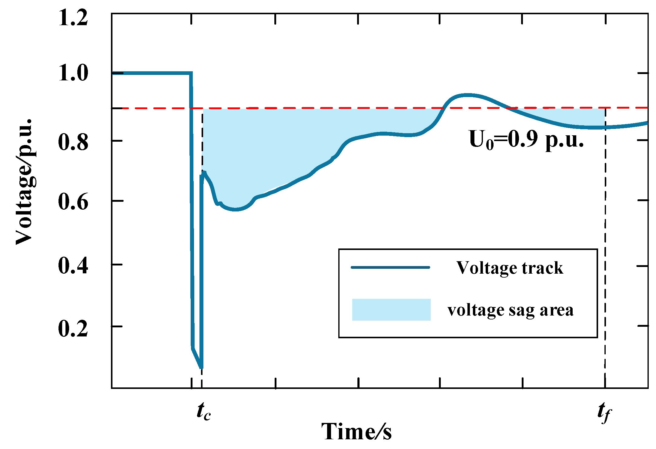
2.2.2. Node Voltage Fluctuation Index

Given the complexity and variability of actual power grid structures and configurations, it becomes increasingly essential to incorporate dynamic and transient features. Following a fault disturbance, nodes across the system exhibit varying degrees of voltage fluctuations. These transient voltage behaviors can be characterized in terms of both fluctuation magnitude and duration. Accordingly, a voltage fluctuation index for each node is defined as follows:

$$U_{\eta }=\left\{\begin{array}{l}{\displaystyle \frac{1-{\displaystyle {\int }_{t_{\mathrm{c}}}^{t_c+\Delta t}S(t)\mathrm{d}t}}{U_0\times \Delta t}},T<T_{th}\\ 0, T\ge T_{th}\end{array}\right.$$

(11)

$$S(t)=\left\{\begin{array}{cc}\left|U(t)-U_0\right|& U(t)\le U_0\\ 0& U(t)>U_0\end{array}\right.$$

(12)

where t_c is the fault clearing moment, Tth is the permissible duration below the transient voltage threshold (taken as 0.75 p.u.), and T is the duration for which the bus voltage is below the threshold in an actual fault. U₀ is the steady voltage amplitude after fault disappearance (U₀ = 0.9).

U_η characterizes the cumulative deviation of node voltage from its steady-state value over a specified period following a disturbance, commonly referred to as the “voltage sag area”. A larger magnitude and longer duration of voltage fluctuation result in a lower value, indicating poorer voltage stability. The schematic illustration is shown in Figure 3.

To facilitate intuitive comparison and analysis of transient voltage characteristics across nodes, a vector-based feature F is constructed to capture the variations in node voltage under different fault scenarios and operating conditions. This feature describes the transient voltage behavior of node i across n scenarios and is defined as follows:

$${\mathit{F}}_i=[{\eta }_{i,1},{\eta }_{i,2},\dots ,{\eta }_{i,n}]\in {\mathbf{R}}^{1\times n}$$

(13)

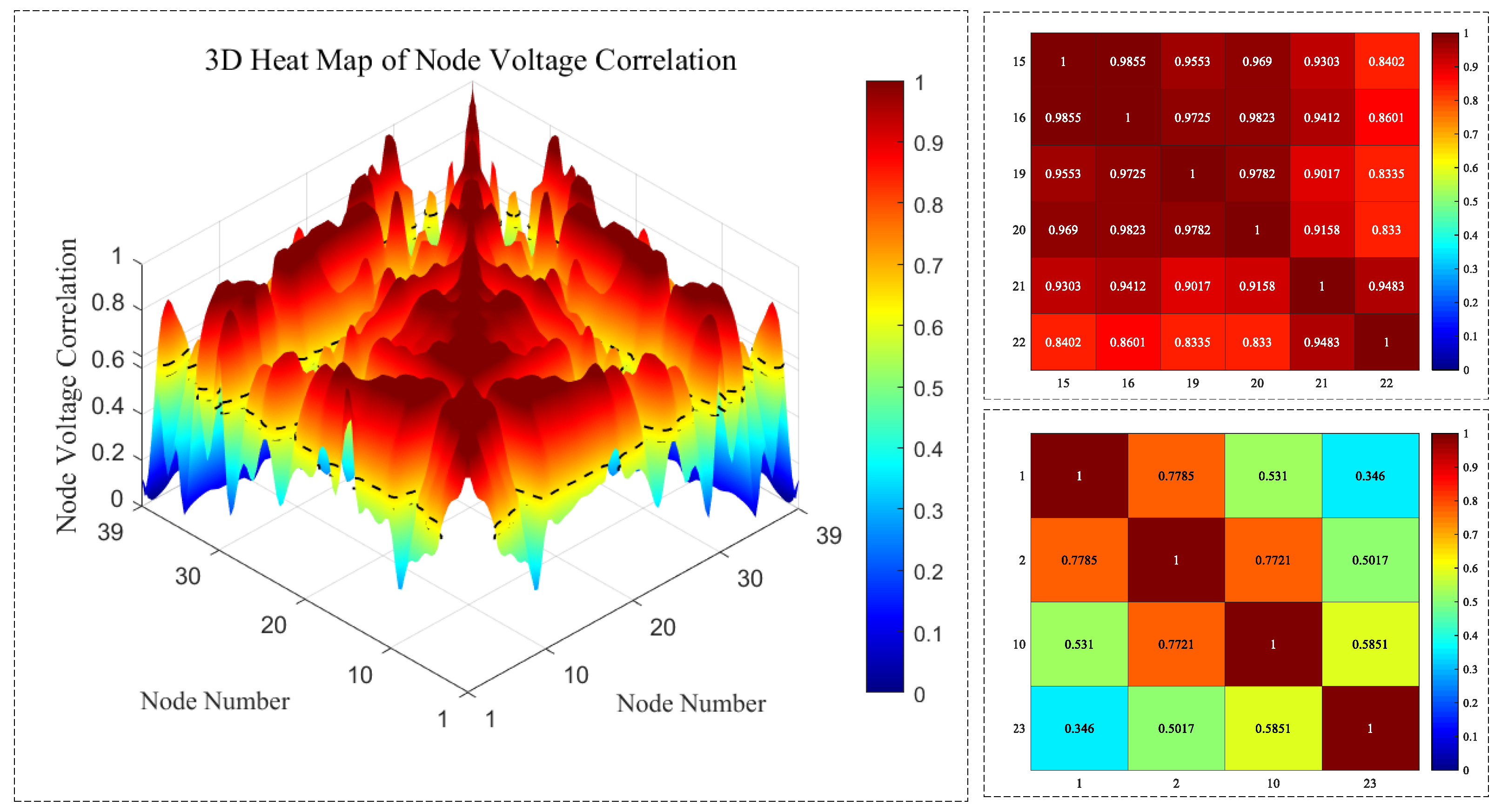
2.3. Weighted Network Considering Node Voltage Correlation

In representing the topological structure of power grids using adjacency matrices, connections between nodes are typically expressed in binary form, using values of 1 or 0 to indicate the presence or absence of a link. However, practical power systems are characterized by non-uniform edge weights as the connections often carry physical and electrical properties beyond simple binary relationships. Traditional adjacent matrix-based models therefore reflect only the existence of connectivity, failing to capture the varying electrical connection between nodes. This limitation restricts the representation of both structural and functional characteristics within the network. To this end, the power grid is modeled as a weighted network G = (V, E, w), where V (G) = {1, 2, ..., n} denotes the set of nodes, E the set of edges, and w the corresponding edge weights. Node voltage correlation is introduced as the weight w, enabling a quantitative description of the electrical closeness between node i and node j.

To quantify feature correlation, metrics such as Euclidean distance, Manhattan distance, and cosine similarity are commonly used. In power systems, voltage waveforms of adjacent nodes tend to exhibit similarity under long-distance faults, despite magnitude differences caused by network impedance. Cosine similarity [25], which measures the angle between vectors and reflects relative variation rather than absolute value, is more suitable for evaluating voltage fluctuation similarity. Accordingly, it is adopted to assess the similarity of transient voltage features, as defined below:

$$\cos (x,y)={\displaystyle \frac{x\cdot y}{\left|x\right|\left|y\right|}}={\displaystyle \frac{{\displaystyle \sum _{i=1}^d}{x}_i{y}_i}{\sqrt{{\displaystyle \sum _{i=1}^d}{x}_i{\overline{x}}_i}\sqrt{{\displaystyle \sum _{i=1}^d}{y}_i{\overline{y}}_i}}},$$

(14)

where ρ ∈ [1, 1]. A higher value of ρ indicates greater similarity, and ρ approaching 1 indicate highly similar directional changes and thus the highest similarity.

By substituting the transient voltage feature vector F, as defined in the previous section, into the above equation, the node voltage correlation can be obtained. This index quantifies the degree of similarity in transient voltage behavior between nodes in the system and is expressed as follows:

$${\rho }_{ij}=\cos ({\mathit{F}}_i,{\mathit{F}}_j)={\displaystyle \frac{{\mathit{F}}_i{\mathit{F}}_j^{\mathrm{T}}}{\left|{\mathit{F}}_i\right|\left|{\mathit{F}}_j\right|}}$$

(15)

Although network partitioning is a widely studied topic, not all available methods are suitable for power grid partitioning. To evaluate the quality of community partitioning in the electrical network, the modularity metric Q is introduced as shown in Equation (16). This metric, originally proposed by Newman, quantifies the difference between the actual density of intra-community edges and the expected density in a comparable randomized network with the same degree distribution. Specifically, a higher value of Q implies stronger community structures with denser internal connections and sparser external connections.

For the complex network shown in Figure 2, the partitioning method based on modularity optimization searches for strong correlations in the network by defining the network holistic partitioning effect index, Q, aggregates the network units from the bottom up, and iterates until the Q value of the network reaches the maximum, thus obtaining the optimal partitioning results, which can effectively solve the problem of determining the number of optimal partitions [15]. Based on node voltage correlation weights, the modularity function Q is employed for power grid partitioning and is defined as follows:

$$Q={\displaystyle \frac{1}{2m}}\sum _{ij}(a{’}_{ij}-{\displaystyle \frac{k_i{k}_j}{2m}})\delta (c_i,c_j)$$

(16)

where m presents the total number of edges, which corresponds to the sum of all edge weights in a weighted network, and a′_ij represents the modified adjacency matrix element based on node voltage correlation. In this study, when nodes i and j are directly connected, a′_ij = ρ_ij. The calculation of ρ_ij is defined in Equation (12). Otherwise, a′_ij = 0; k_i presents the degree of node i, and the calculation of k_i is defined in Equation (3); and c_i presents the community to which node i belongs. When nodes i and j belong to the same community, i.e., c_i = c_j, δ = 1, and otherwise, 0; through this function, the modularity value Q accumulates contributions only from node pairs that belong to the same community.

The modularity metric Q is uniquely determined by the network topology and reflects the deviation between the actual intra-community connectivity and its expected value under a random null model. It has the following key characteristics:

(1)

Value Range: The modularity value Q lies in the interval (0, 1).

(2)

Topological Interpretation: Modularity captures the extent to which connections are concentrated within communities rather than between them. A high Q value indicates that the network exhibits dense intra-community links, while values closer to 0 imply weaker or insignificant community organization.

(3)

Extended Functional Meaning: By adjusting the weights of network edges, modularity can incorporate additional system-level features beyond topology. For example, assigning weights based on electrical correlations allows Q to reflect the functional coupling strength between nodes, rather than just the structural proximity.

Therefore, in this study, the conventional adjacency matrix is modified to embed voltage correlation between nodes into the modularity formulation. This enables the metric to capture both the topological structure and the electrical interaction patterns, making it more suitable for power system partitioning. Overall, modularity offers clear physical interpretability and computational simplicity, making it effective for comparing structural decoupling characteristics across networks. By evaluating different community partitioning schemes within the same network, the optimal number and configuration of partitions can be determined by identifying the maximum Q value.

3. Two-Stage Grid Dynamic Partitioning Strategy

3.1. Pre-Partitioning Based on Electrical Coupling Strength

In power grid partitioning, pre-partitioning plays a key role by reducing dimensionality, guiding the search process, and ensuring physical feasibility. The basic idea of pre-partitioning based on electrical coupling strength used in this paper centers on reactive power source nodes and assigns load nodes to the partition with the highest electrical coupling strength. Connectivity constraints within partitions are maintained via the adjacency matrix, forming the initial partition. Greedy best-first search is referenced during load node assignment, selecting the optimal allocation at each step to achieve efficient partitioning in a single traversal. This approach significantly reduces the computational burden of subsequent community-based partitioning and prevents unrealistic groupings of electrically distant but voltage-similar nodes, thereby improving partitioning accuracy and physical consistency.

As described in Section 2.2.1, the sensitivity of reactive power and voltage is calculated by varying the reactive power injection at source nodes and obtaining the resulting voltage changes at load nodes. For short-circuit impedance distance, a recursive approach is employed to compute the short-circuit impedance Z_ij, and its magnitude is then taken as the electrical distance l_ij. The detailed steps are as follows:

Step 1: For reactive power source node j, assume that it is short-circuit grounded and remove the corresponding row and column from the admittance matrix Y to obtain the Y′.

Step 2: Inject a unit current at load node i while keeping all other injections zero. Compute the V using Equation V = (Y′)⁻¹; V_i represents the short-circuit impedance between nodes j and i.

Step 3: Repeat Step 2 for each load node i to obtain the short-circuit impedances between source node j and all load nodes.

Step 4: Repeat Steps 1–3 for each reactive power source node j until all source–load impedance values are calculated.

Based on the previously obtained sensitivity of reactive power and voltage and the short-circuit impedance distance, the electrical coupling strength can be calculated using Equation (10). This metric is then used as input for pre-partitioning, which proceeds as follows: First, each load node directly connected to a reactive power source node is assigned to the corresponding partition. If multiple load nodes are directly connected, only the one with the highest coupling strength is initially included. Next, load nodes that are either directly connected to the reactive power source node or to any already assigned load node within the same partition, and have the highest coupling strength to that source, are successively incorporated. For every reactive power node, this process is repeated until all load nodes are assigned to initial partitions. As illustrated in Figure 4, for reactive power source node i, among its directly connected nodes h and j, node j exhibits a stronger electrical coupling with node i and is therefore assigned to the partition of source node i. Subsequently, among the nodes directly connected to node j, namely, l, k, and n, node n shows the highest electrical coupling strength with source node i and is thus also included in the same partition.

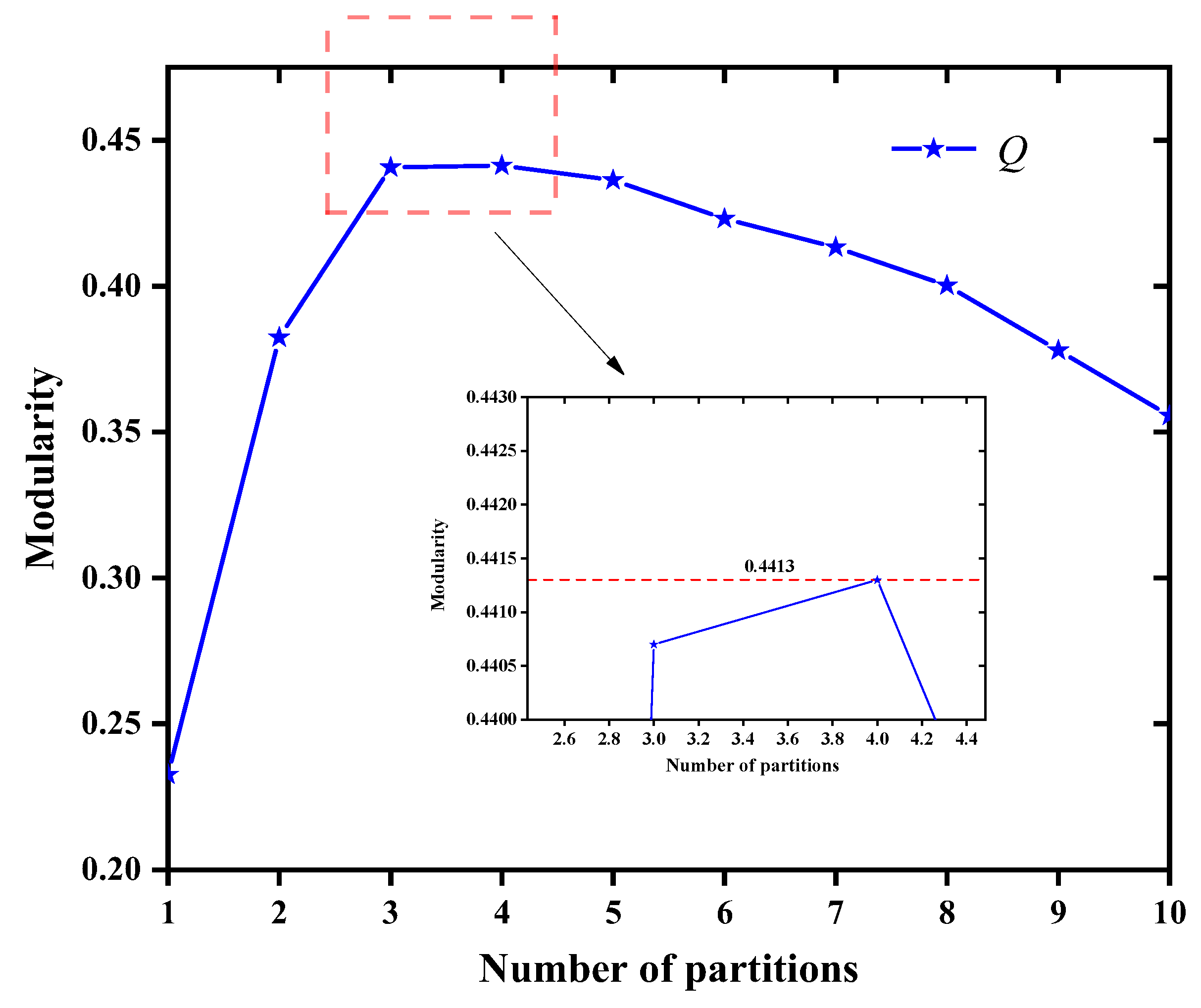
3.2. Second-Stage Partitioning Based on Modularity Optimization

The basic idea of second-stage partitioning is as follows: First, compute the modularity of the initial partition. Then, iteratively merge any two adjacent partitions and recalculate the system modularity. The merging strategy that results in the highest modularity is selected and applied, followed by an update of the modularity metric. This procedure continues until all regions are merged into a single partition. The partitioning Scheme corresponding to the highest modularity after the r-th merge is selected as the final partitioning result. The detailed steps are as follows:

Initial values: n = 10; k = 1 (n and k denote the number of partitions and the number of partitioning methods, respectively).

Step 1: Compute the modularity corresponding to partition scheme k − 1 (k = 1 refers to the initial partition).

Step 2: Select any two partitions (1 ≤ I; j ≤ n) for merging. Calculate the modularity of the resulting configuration and retain the merger that yields the highest modularity.

Step 3: If n ≥ 2, update n = n − 1 and k = k + 1; then, return to Step 1; otherwise, proceed to Step 4.

Step 4: Identify the partitioning scheme with the maximum modularity and designate it as the final partition. The flowchart illustrates two-stage partitioning.

In the second-stage partitioning process, adjacent initial regions are iteratively merged based on the improvement of the overall modularity metric. The adjacency between two regions is determined using the conventional adjacency matrix: two regions are considered adjacent only if there exists at least one direct connection (i.e., an edge) between the nodes belonging to the two regions. This rule ensures that only structurally connected areas are eligible for merging, thereby preventing topologically isolated regions from being erroneously grouped together.

The merging follows a greedy strategy, in which all candidate pairs of adjacent regions are evaluated at each step, and the pair yielding the greatest increase in modularity is selected for merging. This process does not require any predefined number of final partitions or threshold parameters, thus offering flexibility and adaptability to different network structures.

The procedure is repeated until all regions are merged into a single partition. At most, n − 1 merging operations are needed for n initial partitions. In each iteration, the number of candidate region pairs is bounded by n (n − 1)/2, making the approach computationally tractable for medium-scale systems. Among all the intermediate partitioning states generated during this process, the one with the maximum modularity value is identified and selected as the final partitioning result.

A flowchart illustrating the proposed two-stage dynamic partitioning strategy is shown in Figure 5.

4. Case Study

This section first presents the case study setup based on a modified IEEE 39-bus system. The partitioning results obtained using the proposed method are then analyzed and compared with those from existing approaches to demonstrate its effectiveness and advantages.

4.1. Example Setting

A modified IEEE 39-bus system is used as the test case, as illustrated in the Figure 6. In this configuration, synchronous generator 32 is replaced with a wind farm, i.e., generator 34, with a photovoltaic power station, and a DC feeder is connected at bus 8. The system features a renewable energy penetration of 16.86% (10.4% wind and 6.5% solar) and a DC feed-in capacity of 27.5%.

Based on the modified IEEE 39-bus system, various operating scenarios are simulated in the PSD-BPA (version 2.8) by setting different load levels, fault locations (including faulted lines and the percentage distance from the line origin), and fault clearing times. Transient voltage data for all nodes are collected, resulting in a total of 1260 scenarios. The transient voltage characteristics of each node are then calculated and analyzed. On this basis, the proposed two-stage grid partitioning and corresponding performance evaluation are conducted. The specific setting principles are as follows:

(1)

The load level is increased in increments of 10% based on the reference level of 90% to 110%.

(2)

The set of assumed faults is an N − 1 three-phase permanent fault, occurring on a total of 35 buses throughout the system.

(3)

The fault occurs at 0%, 30%, 60%, and 90% of the distance from the line’s starting point.

(4)

The fault clearance time is set to 0.1, 0.2, and 0.3 s after the fault occurs.

4.2. Validation of the Proposed Method

In the modified IEEE 39-bus test system, a total of 10 reactive power source nodes are identified. Based on the methodology described in Section 2, the electrical coupling strength between each reactive power source node and the load nodes is calculated. The results are illustrated in the 3D bar chart shown in Figure 7. Building on this, and following the approach outlined in Section 3.1, load nodes are aggregated around their respective source nodes to form the pre-partitioning scheme. The resulting partition configuration is presented in

Table 1. Pre-partitioning results.

Partition Number	Reactive Power Source	Load Node
1	30	2, 3, 17, 18, 26, 27
2	31	4–7
3	32	10–15
4	33	19
5	34	20
6	35	16, 21, 22, 24
7	36	23
8	37	25
9	38	28, 29
10	39	1, 8, 9

.

Based on the pre-partitioning results, further partition merging is carried out using the method described in Section 3.2, with the objective of maximizing modularity Q. The trend of modularity changes during the merging process is shown in Figure 8, while the detailed merging sequence is illustrated in Figure 9. In this figure, the reactive power source node number represents the corresponding partition, and the number in parentheses (x) indicates the x-th merging operation.

As shown in Figure 9, the highest modularity is achieved after the 6th iteration, reaching a maximum value of 0.4413. The optimal number of partitions is 4, which is in line with the conclusion that the reasonable upper limit of clustering for node-partitioned clustering is $\sqrt{n}$, as derived from the theoretical point of view in Ref. [26]. The final optimal partitioning scheme is illustrated in Figure 10.

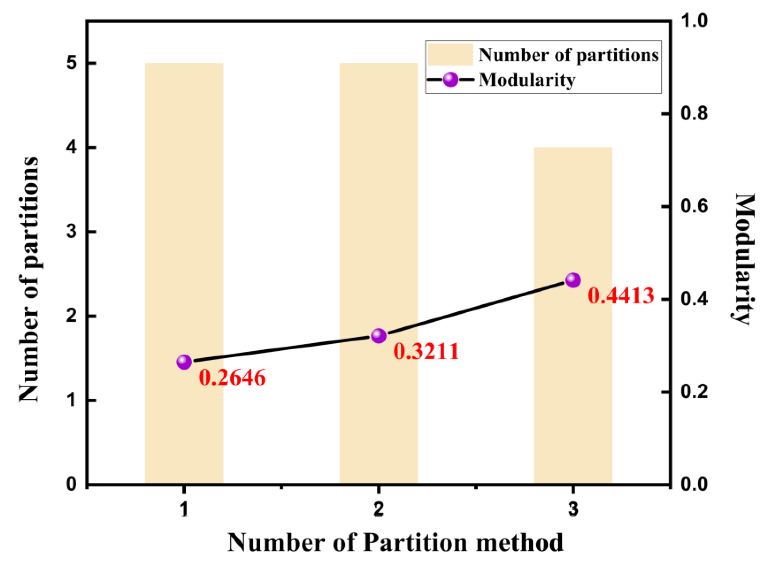
4.3. Comparison and Analysis

For comparison, two existing methods are considered: (1) the partitioning method based on transient voltage feature similarity proposed in Ref. [9] (referred to as the transient voltage-based method); and (2) the method based on reactive power–voltage sensitivity and complex network theory proposed in Ref. [15] (referred to as the complex network-based method). Both approaches have been validated through extensive theoretical analysis and practical applications, demonstrating sound effectiveness and rationality.

4.3.1. Modularity

The partitioning results of all three methods are shown in Figure 11, and the corresponding modularity values for all three methods are presented in Figure 12.

It can be observed that the complex network-based method yields a higher modularity value, indicating superior overall partitioning performance. The proposed two-stage partitioning strategy based on electrical coupling strength achieves the highest modularity, further validating its effectiveness. Moreover, the resulting partition satisfies essential conditions such as regional connectivity, geographical adjacency, and the presence of reactive power sources within each region. Under these constraints, the partitions exhibit high similarity in transient voltage characteristics among internal nodes, clear distinctions between different regions, strong intra-regional coupling, and weak inter-regional interaction.

4.3.2. Regional Decoupling Rate

The regional decoupling rate, as proposed in reference [15] as a metric for evaluating partitioning effectiveness, is uniquely determined by the network topology and specific flow scenarios. This metric provides a comprehensive measure of the decoupling between regions and the internal connectivity within a region. It is widely utilized as a standard for assessing the quality of voltage control partitioning. The formula is as follows:

$$I=\sum _{r=1}^n[{\displaystyle \frac{e_{rr}}{2m}}-{\displaystyle \frac{1}{2}}{({\displaystyle \frac{a_r}{2m}})}^2]$$

(17)

where n represents the total number of regions; e_rr denotes the degree of internal lines within the r-th, defined as twice the sum of the weights of the lines within the region; and a_r represents the degree of lines associated with the r-th region, which is twice the sum of the weights of the lines within the r-th region and those connecting the r-th region to other regions.

The regional decoupling rate ranges from 0 to 0.5. This index holds clear mathematical significance, with the first and second terms representing the cohesion and decoupling of the region, respectively. The subtraction of these two terms reflects the interplay between the internal cohesion and external decoupling. In practical applications, this index is frequently used to evaluate the reasonableness of regional reactive power–voltage decoupling characteristics. The regional decoupling rate specifically emphasizes the decoupling characteristics of “strong internal coupling within regions and weak coupling between regions”. As such, it serves as a valuable complement to the modularity index.

Table 2. The regional decoupling rate for each method.

Partitioning Method	The Regional Decoupling Rate
Transient voltage-based method	0.1702
Complex network-based method	0.2034
Method proposed in this paper	0.2654

presents the regional decoupling rate I for different partitioning methods. The results indicate that the method proposed in this study yields the highest I, which more effectively reflects the decoupling characteristic of “strong internal coupling within regions and weak coupling between regions”.

4.3.3. Maximum Voltage Deviation

Based on node voltage data collected under specific fault scenarios, this study quantitatively assesses the maximum voltage deviation within the partitions for three different partitioning schemes. The specific calculation method is as follows: A specific moment after the fault (in this paper, 10 s following the fault, to compare the steady-state recovery voltage deviation of each node) is selected. At this moment, the voltage difference between all nodes within each subregion is calculated, and the maximum value is taken as the internal maximum voltage deviation of the subregion. Subsequently, the maximum of all internal maximum voltage deviations of the subregions is selected as the maximum voltage deviation for the partitioning scheme.

The results are presented in

Table 3. The maximum voltage deviation for each method.

Partitioning Method	The Maximum Voltage Deviation
Transient voltage-based method	0.0852
Complex network-based method	0.0852
Method proposed in this paper	0.0759

. As shown, the partitioning method proposed in this study achieves the smallest maximum voltage deviation, demonstrating more consistent voltage characteristics. This also provides partial validation of the effectiveness of the node voltage correlation-based partitioning approach introduced in this paper.

To provide a more intuitive comparison of node voltage correlations, as illustrated in the 3D heatmap of node voltage correlation in Figure 13, along with the intra- and inter-partition heatmaps, it is evident that the proposed method yields high voltage similarity and strong coupling among nodes within the same partition, while nodes across different partitions exhibit low transient voltage similarity, indicating near-decoupling between regions. By fully leveraging voltage similarity among nodes, the partitioning approach achieves effective regional separation under geographical and topological constraints, thereby providing a solid theoretical and experimental foundation for subsequent voltage control strategies.

4.4. Limitations and Prospects

In practical applications, several limitations of the proposed method should be acknowledged and addressed in future work:

(1) Limited fault scenarios: This study considers only single-contingency faults, while real-world systems may experience multiple or cascading failures. Extending the method to more complex fault scenarios is essential to improve its robustness and applicability. (2) The inclusion of diverse fault types, locations, and operating conditions increases the computational burden, particularly in large-scale networks: Future efforts may focus on selecting representative fault sets to reduce data dimensionality and mitigate the risk of result degradation caused by overly complex inputs. (3) The assumption of ideal data availability: The method assumes full, accurate, and timely data availability, which may not reflect practical conditions. To improve the practical applicability of the proposed approach, future work may incorporate data uncertainty modeling, robust partitioning strategies, or data-driven estimation techniques to enhance reliability under imperfect information.

5. Conclusions

This study characterizes the electrical coupling strength between reactive power source nodes and load nodes using short-circuit impedance and the sensitivity of reactive power and voltage. Node voltage correlation is constructed based on cosine similarity and incorporated as edge weights to define an undirected weighted graph model of the system. Grid partitioning is then performed by maximizing modularity. The proposed method ensures robustness while accounting for geographical and topological constraints. By fully utilizing voltage similarity among nodes, it achieves the effective decoupling of voltage control across regions and establishes a solid foundation for partition-based voltage regulation. Compared to traditional steady-state-only approaches, the proposed method mitigates sensitivity to power flow conditions and captures transient dynamics. It further ensures that the partitions reflect both voltage behavior and the physical network structure, enhancing the engineering relevance of the results. Future work will focus on applying the method to large-scale power systems. In this context, filtering and selecting representative severe fault scenarios will be essential to reduce computational complexity and data dimensionality, while also avoiding inaccuracy in partitioning results caused by the indiscriminate integration of various fault types.

References

1. Liu, L.; Cheng, H.Z.; Wu, Y.W. Research Progress and Prospects of Transmission Expansion Planning Method for High Proportion of Renewable Energy. Autom. Electr. Power Syst. 2021, 45, 176–183. [Google Scholar]
2. Ruan, H.; Gao, H.; Liu, Y.; Wang, L.; Liu, J. Distributed Voltage Control in Active Distribution Network Considering Renewable Energy: A Novel Network Partitioning Method. IEEE Trans. Power Syst. 2020, 35, 4220–4231. [Google Scholar] [CrossRef]
3. Duan, J.; Li, F.; Xue, B.; Zhu, D.; Wang, H.; Cheng, W. Power Grid Partitioning Methods Based on Improved GN Splitting Algorithm. In Proceedings of the 18th International Conference on AC and DC Power Transmission (ACDC 2022), Virtual, 2–3 July 2022; pp. 725–730. [Google Scholar]
4. Yang, Y.; Sun, Y.; Wang, Q.; Liu, F.; Zhu, L. Fast Power Grid Partition for Voltage Control with Balanced-Depth-Based Community Detection Algorithm. IEEE Trans. Power Syst. 2022, 37, 1612–1622. [Google Scholar] [CrossRef]
5. Chen, J.; Wei, X.; Zhang, T. Advanced Methodology for Optimal Allocation of Reactive Voltage Control Utilizing Sensitivity Matrix Analysis and Distance Evaluation Metrics. In Proceedings of the 2024 IEEE 7th Student Conference on Electric Machines and Systems (SCEMS), Macao, China, 6–8 November 2024; pp. 1–6. [Google Scholar]
6. Li, T.; Xue, F. Power Network Partitioning Method Based on Dijkstra Algorithm. Power Syst. Prot. Control 2018, 46, 159–165. [Google Scholar]
7. Zou, S.H.; Cao, Y.J.; Liu, Z.W. Identification of Grid Weak Link Considering Voltage Instability Patterns at Multiple Time Scales. Power Syst. Prot. Control 2024, 52, 35–49. [Google Scholar]
8. Li, Y.; Cao, Z.; Zhang, Z. Voltage Stability Index-Based Synchronous Condenser Capacity Configuration Strategy of Sending End System Integrated Renewable Energies. In Proceedings of the 2022 IEEE Sustainable Power and Energy Conference (iSPEC), Perth, Australia, 4–7 December 2022; pp. 1–5. [Google Scholar]
9. Jiang, D.; Ma, X.; Liu, Y.; Sun, X.; Chen, Q. Network Partition Method for Transient Voltage Control of the AC/DC Power System. In Proceedings of the 2023 Panda Forum on Power and Energy (Panda FPE), Chengdu, China, 27–30 April 2023; pp. 272–276. [Google Scholar]
10. Liu, Z.; Li, Y.; Yao, L.; Wang, X.; Nie, F. Agglomerative Neural Networks for Multi-View Clustering. IEEE Trans. Neural Netw. Learn. Syst. 2021, 33, 2842–2852. [Google Scholar] [CrossRef]
11. Cao, X.; Han, M.X.; Ma, L.M.; Guo, Z.F.; Cai, W.T.; Zhang, X.H.; Wen, J. Segmentation Method of a Multi-Infeed LCC System Based on Local Fitness Measure. Adv. Technol. Electr. Eng. Energy 2021, 40, 32–42. [Google Scholar]
12. Wang, Y.; Lebovitz, L.; Zheng, K.; Zhou, Y. Consensus Clustering for Bi-Objective Power Network Partition. CSEE J. Power Energy Syst. 2022, 8, 973–982. [Google Scholar]
13. Sinaga, K.P.; Yang, M.S. Unsupervised K-Means Clustering Algorithm. IEEE Access 2020, 8, 80716–80727. [Google Scholar] [CrossRef]
14. Mahdi, S.; Colombo, G.; Longo, M. K-Means and Alternative Clustering Methods in Modern Power Systems. IEEE Access 2023, 11, 119596–119633. [Google Scholar]
15. Peng, X.Y.; Shen, Y.; Lu, Q.Y.; Shen, C. Robust Var-Voltage Control Partitioning for Power Grid Considering Wind Power Uncertainty. Power Syst. Technol. 2023, 47, 4102–4110. [Google Scholar]
16. Zhao, C.; Zhao, J.; Wu, C.; Wang, X.; Xue, F.; Lu, S. Power Grid Partitioning Based on Functional Community Structure. IEEE Access 2019, 7, 152624–152634. [Google Scholar] [CrossRef]
17. Liu, F.; Gu, B.; Qin, S. Power Grid Partition with Improved Biogeography-Based Optimization Algorithm. Sustain. Energy Technol. Assess. 2021, 46, 101267. [Google Scholar] [CrossRef]
18. Zou, Y.; Li, H. Study on Power Grid Partition and Attack Strategies Based on Complex Networks. Front. Phys. 2022, 9, 790218. [Google Scholar] [CrossRef]
19. Zheng, J.X.; Zhong, J. A Complex Network Theory Fast Partition Algorithm of Reactive Voltage Based on Node Type and Coupling of Partitions. Power Syst. Technol. 2020, 45, 223–230. [Google Scholar]
20. Ling, R.; Shao, B.; Li, M.; Chen, X.; Cao, C.; Xue, C. Study of Power Grid Partition Based on the Similarity of Complex Network Communities. Zhejiang Electr. Power 2021, 40, 47–53. [Google Scholar]
21. Wei, Z.B.; Guan, X.Y.; Liu, L.H. Overview of Power Community Structure Discovery Algorithms and Their Application in Power Grid Analysis. Power Syst. Technol. 2020, 44, 2600–2609. [Google Scholar]
22. Massaoudi, M.; Ez Eddin, M.; Ghrayeb, A.; Abu-Rub, H.; Refaat, S.S. Advancing Coherent Power Grid Partitioning: A Review Embracing Machine and Deep Learning. IEEE Open Access J. Power Energy 2025, 12, 59–75. [Google Scholar] [CrossRef]
23. Wang, X.; Xue, F.; Lu, S.; Jiang, L.; Bompard, E.; Masera, M. Understanding Communities from a New Functional Perspective in Power Grids. IEEE Syst. J. 2022, 16, 3072–3083. [Google Scholar] [CrossRef]
24. Yan, W.; Wang, F.; Tang, W.Z. Network Partitioning for Reactive Power/Voltage Control Based on Power Sources Clustering and Short-Circuit Impedance Distance. Power Syst. Prot. Control 2013, 41, 109–115. [Google Scholar]
25. Chen, Y.; Zeng, J.; He, R. Grid Partitioning Method for Medium Voltage Distribution Network Based on Improved K-Means Algorithm. In Proceedings of the 2024 6th International Conference on Eergy, Power and Grid (ICEPG), Guangzhou, China, 27–29 September 2024; pp. 959–962. [Google Scholar]
26. Nguyen, Q.; Ke, X.; Samaan, N.; Holzer, J.; Elizondo, M.; Zhou, H.; Hou, Z.; Huang, R.; Vallem, M.; Vyakaranam, B.; et al. Transmission-Distribution Long-Term Volt-Var Planning Considering Reactive Power Support Capability of Distributed PV. Int. J. Electr. Power Energy Syst. 2022, 138, 107955. [Google Scholar] [CrossRef]
Figure 1. Six-node system schematic diagram.
Energies 18 02544 g001
Figure 2. Community structures schematic diagram.
Energies 18 02544 g002
Figure 3. Voltage sag area schematic diagram.
Energies 18 02544 g003
Figure 4. Schematic diagram of pre-partitioned node consolidation.
Energies 18 02544 g004
Figure 5. Flowchart illustrating two-stage partitioning.
Energies 18 02544 g005
Figure 6. Modified IEEE 39-bus system.
Energies 18 02544 g006
Figure 7. Three-dimensional histogram of electrical coupling strength.
Energies 18 02544 g007
Figure 8. Modularity Q iterative process.
Energies 18 02544 g008
Figure 9. Partition merger process.
Energies 18 02544 g009
Figure 10. Results of the proposed method of partitioning.
Energies 18 02544 g010
Figure 11. Results of the partitioning methods comparing (a) the transient voltage-based method, and (b) the complex network-based method.
Energies 18 02544 g011
Figure 12. Number of partitions and degree of modularity for each method.
Energies 18 02544 g012
Figure 13. Heat map of node voltage correlation.
Energies 18 02544 g013