Research on Missing Data Estimation Method for UPFC Submodules Based on Bayesian Multiple Imputation and Support Vector Machines

Abstract

With the increasing complexity of power systems, the monitoring data of UPFC submodules suffers from high missing rates due to sensor failures and environmental interference, significantly limiting equipment condition assessment and fault warning capabilities. To overcome the computational complexity, poor real-time performance, and limited generalization of existing methods like GRU-GAN and SOM-LSTM, this study proposes a hybrid framework combining Bayesian multiple imputation with a Support Vector Machine (SVM) for data repair. The framework first employs an adaptive Kalman filter to denoise raw data and remove outliers, followed by Bayesian multiple imputation that constructs posterior distributions using normal linear correlations between historical and operational data, generating optimized imputed values through arithmetic averaging. A kernel-based SVM with RBF and soft margin optimization is then applied for nonlinear calibration to enhance robustness and consistency in high-dimensional scenarios. Experimental validation focusing on capacitor voltage, current, and temperature parameters of UPFC submodules under a 50% missing data scenario demonstrates that the proposed method achieves an 18.7% average error reduction and approximately 30% computational efficiency improvement compared to single imputation and traditional multiple imputation approaches, significantly outperforming neural network models. This study confirms the effectiveness of integrating Bayesian statistics with machine learning for power data restoration, providing a high-precision and low-complexity solution for equipment condition monitoring in complex operational environments. Future research will explore dynamic weight optimization and extend the framework to multi-source heterogeneous data applications.

1. Introduction

With the ongoing expansion of power system scales and increasing penetration of renewable energy, modern grids face growing demands for real-time and precise power flow control [1,2]. As a core device in FACTS, the UPFC enhances power transmission efficiency and system stability by dynamically regulating transmission line impedance, voltage magnitude, and phase angle differences [3,4]. Driven by MMC technology, MMC-UPFC has emerged as critical infrastructure in ultra-high-voltage transmission projects due to its modular design, low harmonic output, and high reliability [5,6,7]. However, MMC-UPFC submodule monitoring data face significant challenges in complex operational environments. Firstly, the microsecond-level switching of hundreds of submodules imposes stringent requirements on data acquisition accuracy. Secondly, high-frequency electromagnetic interference and harmonic pollution degrade the signal-to-noise ratio of monitoring data, with typical reductions exceeding 40% under operational conditions [8,9,10]. Additionally, sensor failures and environmental disturbances result in missing rates of 15–20% for critical parameters such as capacitor voltage, current, and temperature, leading to “black module” phenomena that severely hinder equipment condition assessment and fault warning capabilities [11,12].

Current data restoration methods exhibit significant limitations in addressing these challenges. While conventional statistical imputation techniques (e.g., linear interpolation, mean filling) offer computational simplicity, they neglect the spatiotemporal correlations and nonlinear characteristics of power data, resulting in large dynamic restoration errors during transient conditions [13]. Although neural network-based approaches such as GRU-GAN and LSTM can capture complex spatiotemporal dependencies, their training relies on complete datasets, and their high model complexity (e.g., GRU-GAN requiring simultaneous optimization of generators and discriminators) hampers real-time processing on embedded platforms [14,15,16]. Furthermore, traditional multiple imputation techniques reduce uncertainty through multiple imputed values but fail to account for the non-Gaussian distribution characteristics of power data, leading to posterior estimation biases. Additionally, existing methods primarily focus on single-time-scale restoration, lacking adaptability to the multiscale dynamics of UPFC submodules: microsecond-level capacitor voltage fluctuations demand high-precision imputation for real-time control, whereas hour-level temperature trend analysis requires global consistency, posing dual challenges to algorithm robustness and computational efficiency [17,18].

To address the aforementioned issues, this study proposes a hierarchical repair framework based on Bayesian multiple imputation and a Support Vector Machine, which aims to construct an adaptive imputation matrix by establishing a dynamic probabilistic model to analyze the multidimensional operational parameter distribution characteristics of UPFC equipment. While maintaining temporal correlation of data, the framework effectively overcomes the error accumulation problem inherent in traditional methods for power electronic device data repair. Innovatively employing a feature space mapping mechanism, the framework incorporates both the capacitor voltage fluctuation characteristics of UPFC submodules and the switching states of power electronic devices as imputation constraints. This approach achieves enhanced reconstruction accuracy for missing values while maintaining low computational complexity through dimensionality reduction operations, ultimately providing an engineering-practical data preprocessing solution for reliability analysis in flexible AC transmission systems., with core contributions including adaptive data preprocessing through modified Kalman filtering for dynamically adjusting noise covariance matrices to enhance data quality in high-noise scenarios; implementation of multiscale Bayesian multiple imputation that innovatively incorporates discrete-time equations derived from UPFC submodule state–space modeling into posterior distributions and missing value estimation processes, integrating historical data with real-time observations to generate multiple imputation sets while achieving coordinated imputation for transient and sustained missing data through posterior optimization; and nonlinear SVM calibration employing RBF kernels to map high-dimensional feature spaces, utilizing soft-margin optimization to eliminate outliers in imputation results and reinforce physical consistency in restored data. However, it should be noted that the Bayesian multiple imputation method still heavily relies on the completeness and representativeness of the dataset. Specifically, the imputation model constructed in this study imposes strict accuracy constraints on the measured parameters of the MMC-UPFC topology (including submodule capacitance values and arm inductance), where parameter deviations exceeding ±2% will lead to a significant expansion of the confidence intervals in the imputation results.

The first section elucidates the key feature extraction of UPFC submodules, initiating from submodule operating modes by adopting average switching functions to solve MMC submodule characteristic equations and employing the fourth-order Runge–Kutta method for discretization. The second section introduces fundamental principles of Bayesian multiple imputation and the missing value imputation process, incorporating UPFC submodule characteristics. The third section systematically elaborates the Support Vector Machine (SVM)-based calibration methodology for UPFC missing data, which performs secondary calibration and optimization on Bayesian multiple imputation results, with comparative experimental validation demonstrating significant enhancements in high-dimensional data feature resolution and nonlinear relationship modeling accuracy compared to conventional imputation frameworks. The fourth section addresses missing value imputation for UPFC from both short-term and long-term scales to validate the algorithm’s effectiveness.

2. UPFC Submodule Key Data Feature Extraction

2.1. Submodule Modal and Waveform Analysis

Figure 1 illustrates the schematic of a three-phase MMC-UPFC. Each phase arm comprises N SMs adopting a half-bridge configuration, where S1 and S2 represent the switching devices, and C_SM denotes the submodule capacitance. L_o represents the arm filter inductor.

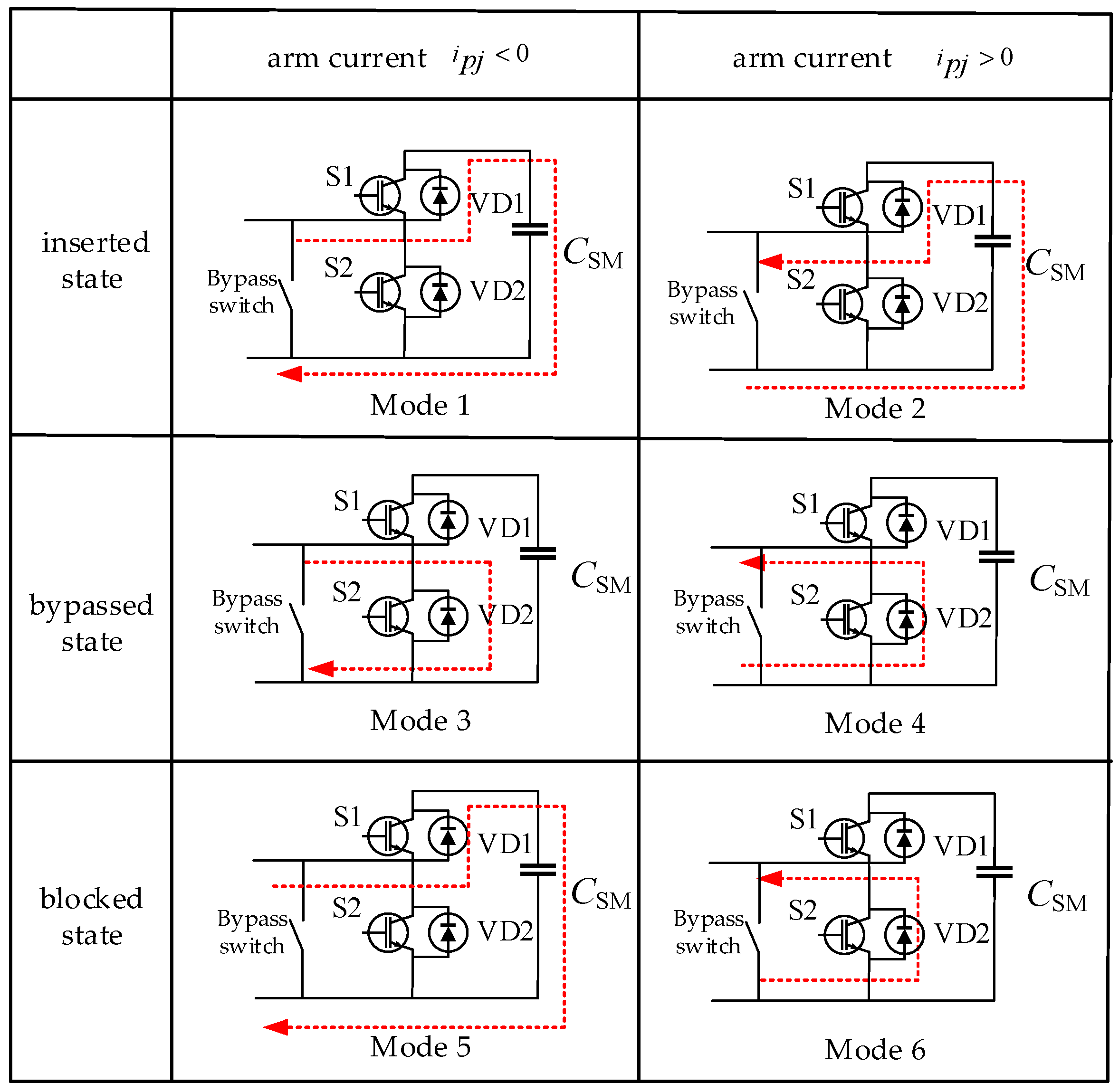
Figure 2 illustrates the operating state diagram of SMs in an MMC-UPFC. SM operational states are categorized into three types: inserted, bypassed, and blocked. In the inserted state, the operation is divided into Mode 1 and Mode 2 based on whether the arm current I_pj is positive (i_pj > 0) or negative. In the bypassed state, switching device T1 remains off while T2 is on, with its operation (Modes 3 and 4) exhibiting an inverse switching configuration compared to the inserted state. For the blocked state, both T1 and T2 are turned off, and SM behavior is entirely dictated by the direction of the arm current, resulting in Modes 5 and 6. The current flow directions for all modes are explicitly indicated in Figure 2.

During operation, the MMC consistently operates in three switching states. For the non-blocked state, the switching functions of the i-th submodule in the upper and lower arms (denoted as p and n) of phase j (j = a, b, c) are defined as follows:

$$S_{SMi,jp(n)}(t)=\left\{\begin{array}{l}1,S=1\\ 0,S=0\end{array}\right.$$

(1)

In the equation, S represents the submodule state, where S = 1 indicates an inserted submodule and S = 0 otherwise. By combining the relational expressions of all submodules in phase j, performing Fourier decomposition on the switching functions of the upper and lower arms while neglecting higher-order harmonic terms, the fundamental-frequency average switching function expressions for the MMC upper and lower arms can be derived as

$$S(t)=\left\{\begin{array}{l}{\displaystyle \frac{1-M\sin ({\omega }_{1}t)}{2}} \mathrm{Upper} \mathrm{arm}\\ {\displaystyle \frac{1+M\sin ({\omega }_{1}t)}{2}} \mathrm{Lower} \mathrm{arm}\end{array}\right.$$

(2)

In the equation, M represents the modulation ratio.

Under CPS-SPWM strategy, the KVL equations for the upper and lower arms in a single-phase unit are formulated as follows:

$$L_{\mathrm{o}}{\displaystyle \frac{d(\frac{1}{2}{i}_{\mathrm{s}j})}{dt}}+L_{\mathrm{o}}{\displaystyle \frac{d{i}_{\mathrm{z}j}}{dt}}=u_{{\mathrm{oo}}^{\prime }}+{\displaystyle \frac{U_{dc}}{2}}-u_{\mathrm{s}j}-u_{\mathrm{p}j}$$

(3)

$$L_{\mathrm{o}}{\displaystyle \frac{d(\frac{1}{2}{i}_{\mathrm{s}j})}{dt}}-L_{\mathrm{o}}{\displaystyle \frac{d{i}_{\mathrm{z}j}}{dt}}=u_{{\mathrm{oo}}^{\prime }}-{\displaystyle \frac{U_{dc}}{2}}-u_{\mathrm{s}j}+u_{\mathrm{n}j}$$

(4)

$$I_{\mathrm{s}j}=I_{\mathrm{n}j}-I_{\mathrm{p}j}$$

(5)

$$I_{\mathrm{z}j}={\displaystyle \frac{P}{3U_{dc}}}={\displaystyle \frac{1}{2}}(I_{\mathrm{n}j}+I_{\mathrm{p}j})$$

(6)

In the equation, the reference point is set as point O, the grid-side power supply reference as point O′, with U_OO^′ representing the voltage between these two points, and L_O denoting the bridge arm inductance value; I_pj and I_nj represent the current amplitudes of the upper and lower arms, respectively; I_sj denotes the amplitude of the grid-side AC current; i_zj is the inter-phase circulating current; I_zj stands for its amplitude; and U_dc corresponds to the DC capacitor voltage.

2.2. Key Data Feature Extraction

Submodule critical data primarily consist of the submodule capacitor voltage and arm input current, as shown in Figure 3. Through analysis of the short-timescale dynamic behavior of UPFC submodules, the mathematical representations of these critical data characteristics can be derived through the integration of switching functions with the KVL equations governing the upper and lower converter arms.

The submodule current i_c, submodule voltage V_c, and submodule capacitor voltage u_c are defined as

$$\begin{array}{l}\left\{\begin{array}{l}{i}_c=S(t)\cdot i_{arm}(t)\\ i_{arm}(t)\approx {\displaystyle \frac{I_{dc}}{3}}-{\displaystyle \frac{I_S}{2}}\cos ({\omega }_{1}t+{\phi }_1)-{\displaystyle \frac{M{I}_S}{4}}\cos ({\omega }_{1}t+{\phi }_2)\end{array}\right.\\ \left\{\begin{array}{l}{V}_c={\displaystyle \frac{U_{dc}}{N}}\\ u_c=V_c-i_c{R}_{esr}={\displaystyle \frac{U_{dc}}{N}}+{\displaystyle \frac{1}{C}}{\displaystyle {\int }_{t=0}^{\infty }{i}_{c}dt}-i_c{R}_{esr}\end{array}\right.\end{array}$$

(7)

In the equation, i_arm denotes the arm current; I_dc/3 represents the DC-side input current; I_S and φ₁ correspond to the magnitude and phase angle of the MMC-UPFC AC-side current; MIs/4 and φ₂ specify the amplitude and phase angle of the second-harmonic circulation component; R_esr denotes the capacitor’s equivalent series resistance; and C_SM denotes the DC-side capacitance value.

Taking the upper arm as an example, the differential expressions governing the submodule capacitor voltage u_c and submodule current i_c are derived from the above relationships as

$$\left\{\begin{array}{l}{\displaystyle \frac{d{u}_c}{dt}}={\displaystyle \frac{1}{C_{SM}}}{i}_c-R_{esr}{\displaystyle \frac{d{i}_c}{dt}}\\ {\displaystyle \frac{d{i}_c}{dt}}=S(t){\displaystyle \frac{d{i}_{arm}(t)}{dt}}+i_{arm}(t){\displaystyle \frac{dS(t)}{dt}}\end{array}\right.$$

(8)

$${\displaystyle \frac{d{u}_c}{dt}}={\displaystyle \frac{1}{C_{SM}}}{i}_c-R_{esr}\left(S(t){\displaystyle \frac{d{i}_{arm}(t)}{dt}}+i_{arm}(t){\displaystyle \frac{dS(t)}{dt}}\right)$$

(9)

The mathematical model of the MMC-UPFC submodule can be discretized via the fourth-order Runge–Kutta method, and the above equation can be expressed as

$$f_1(t,u_c)={\displaystyle \frac{d{u}_c}{dt}}={\displaystyle \frac{1}{C_{SM}}}{i}_c-R_{esr}\left(S(t){\displaystyle \frac{d{i}_{arm}(t)}{dt}}+i_{arm}(t){\displaystyle \frac{dS(t)}{dt}}\right)$$

(10)

The state variable update equations for the next sampling period are formulated as follows:

$$u_{c,n+1}=u_{c,n}+{\displaystyle \frac{h}{6}}(k_{a1}+2k_{a2}+2k_{a3}+k_{a4})$$

(11)

In the equation, h denotes the computational step size and K_a1~K_a4 represent the operational coefficients, with their specific formulas expressed as follows:

$$\left\{\begin{array}{l}{k}_{a1}=f_1(t,u_c)\\ k_{a2}=f_1(t+{\displaystyle \frac{h}{2}},u_c+{\displaystyle \frac{h}{2}}{k}_{a1})\\ k_{a3}=f_1(t+{\displaystyle \frac{h}{2}},u_c+{\displaystyle \frac{h}{2}}{k}_{a2})\\ k_{a4}=f_1(t+h,u_c+h{k}_{a3})\end{array}\right.$$

(12)

The state–space equations can be formulated as

$$u_{c,n+1}=f(C_{SM},R_{esr})\cdot u_{c,n}$$

(13)

3. Submodule Data Imputation Based on Multiple Bayesian Imputation

3.1. Data Acquisition and Preprocessing

Prior to data imputation, preprocessing of UPFC submodule detection data is implemented through Kalman filtering to standardize data formats.

This methodology incorporates cascaded filtering architecture to eliminate both measurement-specific noise from submodule sensors and systemic interference inherent in power electronic systems. Following noise suppression, dynamic threshold determination is executed through historical data averaging, where data points exceeding preset multiples of the mean value are classified as outliers for systematic removal. Multi-sensor redundancy validation ensures measurement reliability by performing cross-correlation analysis on concurrent sampling datasets from identical measurement nodes [19]. The formula of the adaptive Kalman filter is as follows:

$$\left\{\begin{array}{l}{\hat{x}}_{\mathrm{k}}={\hat{x}}_{\mathrm{k}|\mathrm{k}-1}+G_{\mathrm{k}}(z_{\mathrm{k}}-H_{\mathrm{k}}{\hat{x}}_{\mathrm{k}|\mathrm{k}-1})\\ {\hat{x}}_{\mathrm{k}|\mathrm{k}-1}=F_{\mathrm{k}-1}{\hat{x}}_{\mathrm{k}-1}\\ G_{\mathrm{k}}=P_{\mathrm{k}|\mathrm{k}-1}{H}_{\mathrm{k}}^{\mathrm{T}}{(H_{\mathrm{k}}{P}_{\mathrm{k}|\mathrm{k}-1}{H}_{\mathrm{k}}^{\mathrm{T}}/{\beta }_{\mathrm{k}}+R_{\mathrm{k}})}^{-1}/{\beta }_{\mathrm{k}}\\ P_{\mathrm{k}|\mathrm{k}-1}=F_{\mathrm{k}-1}{P}_{\mathrm{k}-1}{F}_{\mathrm{k}-1}^{\mathrm{T}}+Q_{\mathrm{k}-1}\\ P_{\mathrm{k}}=(I-G_{\mathrm{k}}{H}_{\mathrm{k}})P_{\mathrm{k}|\mathrm{k}-1}/{\beta }_{\mathrm{k}}\end{array}\right.$$

(14)

The formula defines the following key parameters of adaptive Kalman filtering: ${\hat{x}}_k$ denotes the estimated state vector at time step k, ${\hat{x}}_{k-1}$ represents the previous estimated state vector, ${\hat{x}}_{k|k-1}$ indicates the one-step predicted state vector, G_k is the adaptive Kalman gain matrix, z_k corresponds to the measurement vector, H_k stands for the measurement matrix, F_k−1 denotes the state transition matrix at step k − 1, P_k|k−1 defines the one-step predicted state error covariance matrix, P_k represents the estimated state error covariance matrix, β_k serves as the adaptive factor, and R_k and Q_k−1, respectively, characterize the measurement noise covariance matrix and process noise covariance matrix, with I being the identity matrix.

The parameter values exceeding the preset multiple of standard deviations from the mean are defined as outliers, where the selection of parameter data points is dynamically adjusted according to the temporal characteristics and variation patterns of the parameter’s operational time scale.

3.2. Bayesian Multiple Imputation

3.2.1. Definition of Missing Values

Following data preprocessing, detection is performed on both operational and historical datasets to identify and locate missing data points, enabling data supplementation and refinement to establish a repaired operational dataset [20].

The UPFC submodule monitoring data comprises missing variables Y and non-missing variables X, including the capacitor voltage, submodule positive terminal voltage, and submodule temperature values. After removing the outliers, historical and operational data are partitioned into equivalent periodic intervals based on state parameters. Each interval is divided into n data points, with the interval length set to correspond to one or multiple cycle durations of the state parameter, adjustable according to data completeness. All complete datasets partitioned under these parameter-specific periodic intervals are aggregated into set X, formatted as an n × q matrix where q denotes the number of complete datasets. Set X represents the non-missing variables in the UPFC submodule monitoring data.

The UPFC submodule monitoring data are represented by missing variable Y, which corresponds to an arbitrarily selected incomplete dataset partitioned according to equivalent periodic intervals of the state parameter. Dataset Y constitutes either a historical dataset with missing entries from a specific time period or an incomplete current operational dataset, serving to characterize the missing variables in the UPFC submodule monitoring data.

The variables Y and X possess a linear relationship characterized by a normal linear correlation between their parameters, expressed as follows:

$$Y~N\left(X\beta ,{\sigma }^2\right)$$

(15)

In the equation, β denotes the regression coefficient, which is a q-dimensional vector, and σ² represents the residual variance.

In dataset Y, the n₁ non-missing observed values are denoted as Y₁, and the corresponding portion of X associated with these observations is labeled X₁. The n₀ artificially created missing values in Y are recorded as Yₘ, with their corresponding X portion designated as Xₘ.

3.2.2. Construction of the Posterior Distribution

Based on the non-missing data portion, the parameters characterizing the relationship between Y and X are estimated, and the posterior distribution of these parameters is constructed. Subsequently, for each missing data point, samples are drawn from this posterior distribution to obtain imputed estimates for the missing values.

In dataset Y, the n₁ non-missing observed values are denoted as Y₁, with their corresponding portion in X labeled X₁; and the n₀ missing values in Y are recorded as Yₘ, with their corresponding X portion is designated Xₘ. Based on the non-missing data subset, estimation is performed using the following formula [21]:

$$\begin{array}{l}{\hat{\beta }}_1={(X_1^T{X}_1)}^{-1}(X_1^T{Y}_1)\\ {\hat{\sigma }}_1^2={(Y_1-X_1{\hat{\beta }}_1)}^T(Y_1-X_1{\hat{\beta }}_1)/(n_1-q)\end{array}$$

(16)

In the equation, ${\hat{\beta }}_1$ denotes the estimated regression coefficients of the model, and ${{\hat{\sigma }}_1}^2$ represents the estimated residuals.

Within the Bayesian framework, the posterior distributions of β and the residuals can be constructed based on OLS estimates. The posterior distribution of the estimated residuals ${\alpha }^2$ chi-square distribution properties are as follows:

$${\displaystyle \frac{{\hat{\sigma }}_1^2}{{\sigma }^2}}(n-q)\sim {\chi }^2(n-q)$$

(17)

In the equation, n represents the number of observed values of state parameters within an equidistant cycle.

The posterior distribution of β depends on the estimated residuals ${\alpha }^2$, following a normal distribution.

3.2.3. Imputation of Missing Values

Missing values are estimated by sampling from the posterior distribution and are combined with the imputed dataset generated by the following imputation model:

$$Y_{*}=X_{\mathrm{m}}{\beta }_{*}+Z_1{\sigma }_{*}$$

(18)

In the equation, $Y_{*}$ is a set of imputed values; σ* is a random sample drawn from the posterior distribution; β* is a random sample drawn from the conditional posterior distribution when $\sigma =\sigma *$; and Z₁ consists of n₀ independent random standard normal variates, expressed as

$${\sigma }_{*}^2={\sigma }_1^2(n_1-q)/g$$

(19)

$${\beta }_{*}={\hat{\beta }}_1+{\sigma }_{*}{({(X_1^T{X}_1)}^{-1})}^{0.5}{Z}_2$$

(20)

In the equation, g is generated by a random draw from χ² (n₁ − q), and Z₂ consists of q independent random standard normal variates.

Considering the critical data characteristics of UPFC submodules, the revised imputation model is formulated as

$${Y_{*}}^{\prime }=Y_{*}+{\lambda }_0{Y}_{comp}$$

(21)

In the equation, λ₀ is the proportionality coefficient derived from the imputation model based on the critical data characteristics of the UPFC submodules; and Y_comp represents the corrected results according to the key physical quantities of the UPFC submodules, where each y_comp,i∈Y_comp is specifically defined as

$$y_{comp,i}=m{\gamma }_{1}f(C_{sm},R_{esr})y(k+1)+{\gamma }_{2}f(C_{sm},R_{esr})y(k-1)i=1,2\dots ,m$$

(22)

In the equation, k represents the position of the i-th missing data in Y_m within the original dataset Y. y(k + 1) and y(k − 1) denote the data at positions k + 1 and k − 1 in Y, respectively; and γ₁ and γ₂ are determined by the time scale and the information status of data at the missing position, where the formula is provided by the state of Equation (13) in Section 2.2. The determination method is illustrated in the Figure 4 below.

The repaired dataset Y′ is obtained by calculating the arithmetic mean of all imputed datasets.

4. SVM-Based Evaluation of Imputed Data

In the formulation, the SVM is a supervised learning algorithm grounded in statistical learning theory, primarily employed for data classification and regression tasks. Its core principle involves locating an optimal hyperplane to separate data of different classes while maximizing the margin, defined as the distance between the hyperplane and the nearest data points [22].

In power system analysis, preprocessed and multiply imputed UPFC data are typically nonlinearly separable. To enable SVMs to process such data, the dataset must be projected into a higher-dimensional space where linear separation becomes feasible. This necessitates the application of kernel techniques in SVMs, whose fundamental principle involves implicitly mapping data to high-dimensional spaces through kernel functions without explicitly computing coordinates in the transformed space. The kernel function essentially computes the inner product between two data points in the high-dimensional space, expressed as

$$K(xi,xj)=\varphi (xi)\cdot \varphi (xj)$$

(23)

In the equation, $\varphi (•)$ represents the mapping function that maps data from the original space into a high-dimensional space.

4.1. SVM-Based Data Calibration

The repaired operational dataset is denoted as Y′. For a given set of data points (x_i, y_i) where i = 1, 2, …, l, with x_i ∈ Y′ and y_i ∈ {−1, 1}, an optimal hyperplane can be identified to separate the samples when linear separability is achieved, mathematically represented as

$$w^{T}x+b=0$$

(24)

In the equation, w and b represent the weight vector and the optimal hyperplane offset, respectively. The optimal hyperplane is shown in Figure 5 below.

The SVM method utilizes soft margin optimization and kernel tricks to map samples from the original space into a high-dimensional feature space. Within this high-dimensional space, the SVM identifies a maximum-margin linear hyperplane for data classification. This linear hyperplane is formulated by solving the following optimization problem:

$$\left\{\begin{array}{l}\underset{w,b}{\min } {\displaystyle \frac{1}{2}}{‖w‖}^2+C{\displaystyle \sum _{i=1}^m{\xi }_i}\\ \mathrm{s}.\mathrm{t}. y_i[w^T\cdot \phi (x_i)+b]\ge 1-{\xi }_i,{\xi }_i\ge 0,i=1,\dots ,m\end{array}\right.$$

(25)

In the above equation, C > 0 denotes the penalty factor, ξ_i represents the slack variable, and $\phi (x_i)$ corresponds to the feature vector of x_i mapped into the high-dimensional space. In the calculation process of the above equation, $\phi {(x_i)}^T\phi (x_i)$ needs to be solved. It is solved by using the kernel function [23]. In the Support Vector Machine (SVM) method, there are four types of kernel functions, which are mathematically defined as follows:

$$\left\{\begin{array}{l}\mathrm{linear}:K(x_i,x_j)={x_i}^{T}x\\ \mathrm{polynomial}:K(x_i,x_j)={(\gamma {x_i}^{T}x+r)}^d,\gamma >0\\ \mathrm{RBF}:K(x_i,x_j)=\exp (-\gamma {‖x_i-x‖}^2),\gamma >0\\ \mathrm{sigmoid}:K(x_i,x_j)=\tanh (\gamma {x_i}^{T}x+r)\end{array}\right.$$

(26)

In the above equation, r, γ, and d are all kernel parameters.

4.2. The Advantages of Applying Support Vector Machines (SVMs) to UPFC Submodule Imputation

For sensor data such as UPFC submodules, which typically consist of multi-parameter and multi-dimensional numerical values, SVMs implicitly map such data into high-dimensional spaces via the kernel trick, making them suitable for handling high-dimensional features. Even when the feature dimensionality far exceeds the sample size, SVMs can maintain generalization performance by maximizing the margin, thereby avoiding the “curse of dimensionality”.

UPFC data involve complex nonlinear relationships such as coupling between voltage and power. SVMs can effectively capture these relationships using nonlinear kernel functions like the Gaussian kernel, thereby further improving imputation accuracy. If redundant features exist in high-dimensional data, SVM feature weights (e.g., linear kernel coefficients) can be utilized to screen critical variables, enhancing imputation efficiency.

5. Case Analysis

5.1. Data Source

5.1.1. Short-Time-Scale Data Sources

Simulation data were acquired through PLECS-based modeling of the UPFC, with the corresponding simulation model configuration depicted in the following Figure 6 and critical operational parameters specified in the accompanying

Table 1. Key parameters.

Parameter Name	Value
Number of Submodules (N)	20
AC-side Voltage Frequency (fg)	50 Hz
AC-side Line Voltage Amplitude (Ugm)	500 kV
DC Bus Total Reference Voltage (Udc)	180 kV
DC Capacitor Initial Voltage per Submodule (Usm)	Udc/N (kV)
Submodule Capacitance (Csm)	11 × 10−3 F
DC Bus Capacitance (Carm)	100 × 10−6 F
Filter Inductance (Larm)	36 × 10−3 H
Filter Winding Resistance (Rarm)	0.1 Ω
Equivalent Inductance (Lg)	1.00 × 10−3 H
Equivalent Resistance (Rg)	0.1 Ω
Carrier Ratio (FR)	2.4
Triangular Carrier Frequency (fsw)	Fg × FR Hz
Line Inductance (Ln)	0.001 H
Line Resistance (Rn)	1 Ω
Line Capacitance (CL)	1.00 × 10−5

:

The simulation parameters are configured as follows: The UPFC series-side capacity is 250 × 2 MVA, with the shunt-side capacity set at 250 MVA and an AC bus voltage regulation range spanning 485 kV to 535 kV. The maximum operating voltage at the converter valve-side reaches 105 kV for the series unit and 94 kV for the shunt unit, while the DC-side maintains a rated voltage of 90 kV with a maximum operational voltage of 92.5 kV. This configuration strictly adheres to IEC 61803 standards for power electronic converter testing.

5.1.2. Long-Term Time-Scale Data Source

The long-term time-scale data source originates from real UPFC phasor measurement data, where the phasor measurement data are selected from 1 October 2023, as shown in Figure 7.

5.2. Process Framework

Figure 8 illustrates the framework of the data restoration process. Time scales are distinguished based on data sampling intervals. When short-term time-scale data are identified, missing data restoration is executed by integrating key operational characteristics of UPFC submodules with numerical analysis methods. For long-term time-scale missing data scenarios where UPFC circuit intrinsic characteristics become non-manifested, data imputation is exclusively performed through numerical analysis methods.

5.3. Imputation Data Accuracy Validation Metrics

Following data imputation, a comprehensive accuracy assessment between the imputed and original datasets was performed using four statistical parameters—Mean Squared Error (MSE), Mean Absolute Error (MAE), Pearson correlation coefficient (r), and Coefficient of determination (R²)—to evaluate the precision of the imputation results.

The MSE quantifies the average squared deviation between imputed and true values, demonstrating sensitivity to significant errors with its optimal value approaching zero. The MAE measures the absolute average magnitude of imputation errors, providing intuitive error magnitude interpretation, where values below 15% of the standard deviation indicate satisfactory performance. The r evaluates linear correlation strength between imputed and true values, with absolute values exceeding 0.8 denoting strong correlation and values below this threshold suggesting weak correlation. The R² reveals the explanatory power of imputed values for true value fluctuations, where values above 0.9 signify excellent model fitting, values between 0.7 and 0.9 indicate adequate explanatory capability, and values below 0.7 reflect suboptimal fitting performance. The calculation formulas for specific parameters are listed in

Table 2. Calculation formula for accuracy index.

Name of Parameter	Formula
Mean Squared Error (MSE)	$\mathrm{MSE}={\displaystyle \frac{1}{n}}{\displaystyle \sum _{i=1}^n{(y_i-{\hat{y}}_i)}^2}$
Mean Absolute Error (MAE)	$\mathrm{MAE}={\displaystyle \frac{1}{n}}{\displaystyle \sum _{i=1}^n|}{y}_i-{\hat{y}}_i|$
Pearson correlation coefficient (r)	$r={\displaystyle \frac{{\displaystyle \sum _{i=1}^n(x_i-\overline{x})}(y_i-\overline{y})}{\sqrt{{\displaystyle \sum _{i=1}^n{(x_i-\overline{x})}^2}}\cdot \sqrt{{\displaystyle \sum _{i=1}^n{(y_i-\overline{y})}^2}}}}$
Coefficient of determination (R2)	$R^2=1-{\displaystyle \frac{{\displaystyle \sum _{i=1}^n{(y_i-{\hat{y}}_i)}^2}}{{\displaystyle \sum _{i=1}^n{(y_i-\overline{y})}^2}}}$

below.

In the formula, n represents the number of data points, y_i is the true value, ${\hat{y}}_i$ is the predicted value, and $\overline{y}$ is the average value of the true values.

5.4. Short-Term Time-Scale Imputation Performance

Three symbolic variables were defined to represent submodule voltage (u_c), submodule current (i_SM), and submodule temperature (T_SM). The algorithm parameters were configured with minimum/maximum iteration limits of 50 and 1000, respectively, a termination tolerance of 1 × 10⁻⁹, and an intentional 50% missing data ratio per dataset to simulate extreme operational conditions.

5.4.1. Bayesian Multiple Imputation for Submodule Current (i_c)

A comparison of conventional linear imputation and Bayesian multiple imputation results is depicted below Figure 9.

5.4.2. Bayesian Multiple Imputation for Submodule Voltage (u_c)

A comparative analysis of reconstruction accuracy across distinct imputation regimes is shown below Figure 10.

The interpolation accuracy of sub-module data is shown in

Table 3. Sub-module data imputation accuracy.

Indicators	Submodule Current ic		Submodule Voltage uc
	Linear Imputation	Multivariate Imputation	Linear Imputation	Multivariate Imputation
MSE	18,560.2328	59.6838	258.7016	9.7597
MAE	62.9265	4.9329	5.9061	1.3709
r	0.9894	1.0000	0.9937	0.9998
R2	0.9790	1.0000	0.9874	0.9995

.

Under 50% missing data conditions, the simulation results in Figure 9 and Figure 10 and associated metric calculations presented in Table 2 demonstrate that both linear and multivariate interpolation methods for submodule current (i_c) and voltage (u_c) achieve correlation coefficients (r) and R² values within the 0.9–1.0 range, indicating strong fitting relationships with raw data and sufficient model explanatory power, with multivariate interpolation outperforming linear interpolation. However, during MSE and MAE evaluation, linear interpolation exhibits significantly larger errors, manifesting pronounced sawtooth waveform distortions in the simulation model, demonstrating substantially lower accuracy compared to multivariate interpolation results.

5.4.3. Bayesian Multivariate Interpolation for AC-Side Single-Phase Current (i_pa)

A comparison of conventional linear imputation and Bayesian multiple imputation results is shown below Figure 11.

5.4.4. Bayesian Multivariate Interpolation for AC-Side Single-Phase Voltage (u_sc)

A comparative analysis of reconstruction accuracy across distinct imputation regimes is shown below Figure 12.

The interpolation accuracy of the bridge arm data is presented in

Table 4. Arm data imputation accuracy.

Indicators	AC-Side-Current ipa		AC-Side Voltage usc
	Linear Imputation	Multivariate Imputation	Linear Imputation	Multivariate Imputation
MSE	91,054.7895	15.0950	2,760,691.3427	35,351.3849
MAE	151.8561	2.3564	8909.3717	118.2776
r	0.9981	1.0000	0.9983	1.0000
R2	0.9962	1.0000	0.9967	1.0000

.

Under 50% missing data conditions, the simulation results from Figure 11 and Figure 12 and corresponding metric calculations in Table 3 reveal that both linear and multivariate interpolation methods for submodule voltage and current demonstrate strong fitting performance, with correlation coefficients (r) and R² values within the 0.9–1.0 range, consistent with previous interpolation outcomes. The multivariate interpolation model exhibits exceptional proximity to the original data pattern due to the substantial sampling dataset. In MSE and MAE evaluations, multivariate interpolation significantly outperforms linear interpolation, achieving superior accuracy with minimal error margins.

5.5. Long-Term Timescale Imputation Performance

5.5.1. Bayesian Multivariate Interpolation for Submodule Voltage (u_c) and Current (i_c)

Under constant load conditions, the submodule voltage u_c and current i_c exhibit quasi-constant waveforms over long-term time scales due to their high switching frequency characteristics, as shown in Figure 13. However, actual UPFC field operations involve daily load fluctuations (as exemplified in telemetry data, Figure 7), granting operational telemetry data significant statistical relevance for validating analytical methodologies. This positions the daily operational dataset as a robust validation source for extended-duration performance verification in practical power electronics systems.

5.5.2. Bayesian Multivariate Interpolation for Telemetry Current (i_SM)

A comparison of the results of ordinary linear interpolation, built-in Makima interpolation, cubic spline interpolation, and Bayesian multiple imputation is shown below Figure 14.

The interpolation accuracy of the actual telemetry current data is shown in

Table 5. Telemetry current i_SM data imputation accuracy.

Indicators	Linear Imputation	Makima Imputation	Cubic Spline Interpolation	Multivariate Imputation
MSE	17.9862	0.2189	0.4407	0.1926
MAE	2.1205	0.2236	0.3588	0.2034
r	0.8791	0.9867	0.9975	1.0000
R2	0.7727	0.9774	0.9950	1.0000

.

5.5.3. Bayesian Multivariate Interpolation for Telemetry Voltage (u_SM)

A comparison of the results of ordinary linear interpolation, built-in Makima interpolation, cubic spline interpolation, and Bayesian multiple imputation is shown below Figure 15.

The interpolation accuracy of the actual telemetry voltage data is shown in

Table 6. Telemetry current u_SM data Imputation accuracy.

Indicators	Linear Imputation	Makima Imputation	Cubic Spline Interpolation	Multivariate Imputation
MSE	0.002	0.0013	0.0004	0.0001
MAE	0.0238	0.0035	0.0099	0.0004
r	0.8329	0.9952	0.9748	1.0000
R2	0.6936	0.9904	0.9503	1.0000

.

5.5.4. Bayesian Multivariate Interpolation for Telemetry Temperature (T_SM)

A comparison of the results of ordinary linear interpolation, built-in Makima interpolation, cubic spline interpolation, and Bayesian multiple imputation is shown below Figure 16.

The interpolation accuracy of the telemetry temperature data is shown in

Table 7. Telemetry temperature T_SM imputation accuracy.

Indicators	Linear Imputation	Makima Imputation	Cubic Spline Interpolation	Multivariate Imputation
MSE	5.5518	0.1563	0.9241	0.0141
MAE	1.3320	0.1883	0.4986	0.0167
r	0.8329	0.9958	0.9783	0.9981
R2	0.6556	0.9916	0.9571	0.9978

.

Under extended-duration time frames, comparative interpolation analyses were conducted on telemetry submodule current i_SM, voltage u_c, and temperature T_SM parameters using linear imputation, Makima imputation, cubic spline interpolation, and Bayesian multivariate interpolation methods. Simulation comparisons with precision metric calculations revealed distinct performance characteristics: linear interpolation demonstrated limited effectiveness, only updating data points adjacent to missing values while introducing significant deviations from original data patterns. Makima imputation and Cubic spline interpolation achieved approximate restoration of baseline data models but exhibited partial reconstruction inaccuracies. In contrast, Bayesian multivariate interpolation precisely reconstructed all three data parameters with fidelity to original operational signatures, experimentally validating its reliability for power electronics telemetry restoration tasks.

5.6. Support Vector Machine (SVM) Hyperparameter Optimization Outcomes

The missing data ratio for three-category symbolic data was controlled at 9.4%, with confidence intervals of 63.5%, 24.4%, and 12.1%, respectively, as illustrated in Figure 17.

In the SVM optimization section, the model results under 50% missing data conditions are shown in the figure. The proposed Bayesian multiple imputation combined with SVM methodology demonstrates controlled missing ratios (9.4% for three-category symbolic data) with confidence intervals of 63.5%, 24.4%, and 12.1%, respectively.

6. Conclusions

This study implements Bayesian multiple imputation combined with SVM optimization for UPFC submodule state information processing. Through standardized preprocessing of operational and historical submodule data, we first localize missing data points, then perform multi-stage imputation specifically tailored for short-term and long-term temporal scales of UPFC submodules, thereby validating the feasibility of Bayesian multiple imputation methodology.

Under short-term time scale validation, this study comparatively analyzed the Bayesian multiple imputation method integrated with UPFC submodule key characteristic data against conventional linear interpolation, with precision evaluated through four metrics: MSE, MAE, r, and R². Both methods demonstrated competent performance in data fitting and correlation preservation due to high-density sampling points, yet the conventional linear interpolation exhibited substantially higher model recovery errors owing to its reliance solely on adjacent data points. Extended missing-value imputation simulations on UPFC arm current–voltage parameters further confirmed the systematic superiority of the Bayesian method in both error suppression and fitting accuracy.

For long-term time scale verification, a comparative study was conducted across four methods: conventional linear interpolation, MAKIMA interpolation, cubic spline interpolation, and Bayesian multiple imputation. Through missing-value simulations on telemetric arm current, voltage, and temperature data, the results revealed that conventional linear interpolation failed in data fitting due to insufficient global data correlation modeling; Makima and cubic spline methods partially reconstructed data trends but retained notable residual errors; whereas the Bayesian multiple imputation achieved optimal precision in missing-value reconstruction through probabilistic dataset generation and posterior distribution modeling, outperforming other methods in both fitting fidelity and error minimization.

The methodology demonstrates universal applicability that meets the practical requirements for UPFC submodule condition monitoring. The restored dataset is subsequently integrated with SVM-based anomaly detection to identify abnormal imputation points, enabling iterative data updates that form operational datasets with enhanced estimation accuracy. The algorithm achieves improved repair precision with low computational complexity, significantly enhancing data restoration reliability while ensuring data integrity.

References

- Tang, Z.; Yang, Y.; Blaabjerg, F. Power electronics: The enabling technology for renewable energy integration. CSEE J. Power Energy Syst. 2022, 8, 39–52. [Google Scholar]
- Gu, Y.; Huang, Y.; Wu, Q.; Li, C.; Zhao, H.; Zhan, Y. Isolation and Protection of the Motor-Generator Pair System for Fault Ride-Through of Renewable Energy Generation Systems. IEEE Access 2020, 8, 13251–13258. [Google Scholar] [CrossRef]
- Elsaharty, M.A.; Luna, A.; Candela, J.I.; Rodriguez, P. A Unified Power Flow Controller Using a Power Electronics Integrated Transformer. IEEE Trans. Power Deliv. 2019, 34, 828–839. [Google Scholar] [CrossRef]
- Lei, Y.; Li, T.; Tang, Q.; Wang, Y.; Yuan, C.; Yang, X.; Liu, Y. Comparison of UPFC, SVC and STATCOM in Improving Commutation Failure Immunity of LCC-HVDC Systems. IEEE Access 2020, 8, 135298–135307. [Google Scholar] [CrossRef]
- Cheng, T.; Zhong, J.; Yang, B.; Wei, Y.; Xu, J.; Zhang, Z. Improved Circulation Suppression Strategy for MMC Considering Low Frequency Oscillation. In Proceedings of the 2021 11th International Conference on Power and Energy Systems (ICPES), Shanghai, China, 18–20 December 2021; pp. 57–61. [Google Scholar]
- Huang, H.; Zhang, L.; Oghorada, O.; Mao, M. Analysis and Control of a Modular Multilevel Cascaded Converter-Based Unified Power Flow Controller. IEEE Trans. Ind. Appl. 2021, 57, 3202–3213. [Google Scholar] [CrossRef]
- Biswas, S.; Nayak, P.K. A Fault Detection and Classification Scheme for Unified Power Flow Controller Compensated Transmission Lines Connecting Wind Farms. IEEE Syst. J. 2021, 15, 297–306. [Google Scholar] [CrossRef]
- Ji, S.; Huang, X.; Palmer, J.; Wang, F.; Tolbert, L.M. Modular Multilevel Converter (MMC) Modeling Considering Submodule Voltage Sensor Noise. IEEE Trans. Power Electron. 2021, 36, 1215–1219. [Google Scholar] [CrossRef]
- Dai, K.; Luo, H.; Yang, H.; He, K.; Xu, Z.; Jin, P.; Cai, H.; Xu, C. PCC Voltage Switching Harmonic Mitigation by Periodic Carrier Frequency Pulsewidth Modulation for SiC High-Frequency Active Power Filter. IEEE J. Emerg. Sel. Top. Power Electron. 2024, 12, 3040–3051. [Google Scholar] [CrossRef]
- Wu, Q.; Zhu, Z.; Zhou, M.; Li, C.; Zhu, X. Research on Data Acquisition Method of Power System Based on Compressed Sensing Technology. In Proceedings of the 2024 2nd International Conference on Pattern Recognition, Machine Vision and Intelligent Algorithms (PRMVIA), Changsha, China, 24–27 May 2024; pp. 141–144. [Google Scholar]
- Liu, X.; Zhang, Z. A Two-Stage Deep Autoencoder-Based Missing Data Imputation Method for Wind Farm SCADA Data. IEEE Sens. J. 2021, 21, 10933–10945. [Google Scholar] [CrossRef]
- Liu, Y.; Duan, Z.; Hu, P.; Hu, C.; Zheng, J.; Li, Z. MMC Submodule Topology With CVSB and DCFRT Capability for Offshore Wind Farms Black-Start. IEEE Trans. Ind. Appl. 2024, 60, 2891–2900. [Google Scholar] [CrossRef]
- Zhou, K.; Gao, F.; Zhang, Y.; Hou, Z.; Nie, K.; Xu, T.; Wang, H.; Xu, K. Missing Data Imputation for Photovoltaic Station Based on Spatiotemporal Features. In Proceedings of the 2024 CPSS & IEEE International Symposium on Energy Storage and Conversion (ISESC), Xi’an, China, 8–11 November 2024; pp. 355–359. [Google Scholar]
- Yang, Y.; Wang, W.; Zhong, Y.; Jin, C.; Zhao, C.; Qiu, B.; Jia, W. Short-Term EVs Charging Load Prediction Under Low-quality Data Environment Based on GRU-GAN-GOA-MKELM Framework. In Proceedings of the 2024 International Seminar on Artificial Intelligence, Computer Technology and Control Engineering (ACTCE), Wuhan, China, 28–29 September 2024; pp. 145–152. [Google Scholar]
- Kim, J.; Lee, J. Statistical Classification of Vehicle Interior Sound Through Upsampling-Based Augmentation and Correction Using 1D CNN and LSTM. IEEE Access 2022, 10, 100615–100626. [Google Scholar] [CrossRef]
- Lee, S.-Y.; Connerton, T.P.; Lee, Y.-W.; Kim, D.; Kim, D.; Kim, J.-H. Semi-GAN: An Improved GAN-Based Missing Data Imputation Method for the Semiconductor Industry. IEEE Access 2022, 10, 72328–72338. [Google Scholar] [CrossRef]
- Allella, F.; Chiodo, E.; Giannuzzi, G.M.; Lauria, D.; Mottola, F. On-Line Estimation Assessment of Power Systems Inertia With High Penetration of Renewable Generation. IEEE Access 2020, 8, 62689–62697. [Google Scholar] [CrossRef]
- Zhao, Z.; Luo, X.; Wu, J.; Xie, J.; Gong, S.; Ni, Q.; Lai, C.S.; Lai, L.L. Model Reduction for Grid-Forming Hybrid Renewable Energy Microgrid Clusters Based on Multi-Timescale Characterization. IEEE Trans. Smart Grid 2024, 15, 1227–1242. [Google Scholar] [CrossRef]
- Liu, H.; Hu, F.; Su, J.; Wei, X.; Qin, R. Comparisons on Kalman-Filter-Based Dynamic State Estimation Algorithms of Power Systems. IEEE Access 2020, 8, 51035–51043. [Google Scholar] [CrossRef]
- Ahmed, H.M.; Abdulrazak, B.; Blanchet, F.G.; Aloulou, H.; Mokhtari, M. Long Gaps Missing IoT Sensors Time Series Data Imputation: A Bayesian Gaussian Approach. IEEE Access 2022, 10, 116107–116119. [Google Scholar] [CrossRef]
- Lei, M.; Labbe, A.; Wu, Y.; Sun, L. Bayesian Kernelized Matrix Factorization for Spatiotemporal Traffic Data Imputation and Kriging. IEEE Trans. Intell. Transp. Syst. 2022, 23, 18962–18974. [Google Scholar] [CrossRef]
- Sun, P.; Liu, X.; Lin, M.; Wang, J.; Jiang, T.; Wang, Y. Transmission Line Fault Diagnosis Method Based on Improved Multiple SVM Model. IEEE Access 2023, 11, 133825–133834. [Google Scholar] [CrossRef]
- Gong, X.; Zou, B.; Duan, Y.; Xu, J.; Luo, Q.; Yang, Y. Multiple Kernel SVM Based on Two-Stage Learning. IEEE Access 2020, 8, 101133–101144. [Google Scholar] [CrossRef]
Figure 1.
Three-phase MMC-UPFC topological schematic diagram.
Figure 2.
MMC submodule operating modes.
Figure 3.
Detailed submodule topology.
Figure 4.
Missing value imputation process framework.
Figure 5.
Support vector machine optimal hyperplane.
Figure 6.
UPFC operational topology for simulation.
Figure 7.
(a) The telemetry voltage measurements, and (b) the telemetry current measurements recorded on 1 October 2023.
Figure 8.
Data restoration process framework.
Figure 9.
The interpolation results for submodule current ic are shown in (a) using linear interpolation and in (b) employing Bayesian multiple imputation.
Figure 10.
The interpolation results for submodule voltage uc are shown in (a) using linear interpolation and in (b) employing Bayesian multiple imputation.
Figure 11.
The interpolation results for AC-side single-phase current ipa are shown in (a) using linear interpolation and in (b) employing Bayesian multiple imputation.
Figure 12.
The interpolation results for AC-side single-phase voltage usc are shown in (a) using linear interpolation and in (b) employing Bayesian multiple imputation.
Figure 13.
(a) The operational waveform of submodule voltage uc, and (b) the operational waveform of submodule current ic.
Figure 14.
The interpolation results for telemetry current iSM are presented in (a) using linear interpolation, in (b) with the built-in Makima interpolation, in (c) with the cubic spline interpolation, and (d) through Bayesian multiple imputation.
Figure 15.
The interpolation results for telemetry voltage uSM are presented in (a) using linear interpolation, in (b) with the built-in Makima interpolation, in (c) with the cubic spline interpolation, and (d) through Bayesian multiple imputation.
Figure 16.
The interpolation results for telemetry temperature TSM are presented in (a) using linear interpolation, in (b) with the built-in Makima interpolation, in (c) with the cubic spline interpolation, and (d) through Bayesian multiple imputation.
Figure 17.
Model under 50% missing data condition.