Research on Shale Oil Well Productivity Prediction Model Based on CNN-BiGRU Algorithm

Abstract

Unconventional reservoirs are characterized by intricate fluid-phase behaviors, and physics-based shale oil well productivity prediction models often exhibit substantial deviations due to oversimplified theoretical frameworks and challenges in parameter acquisition. Under these circumstances, data-driven approaches leveraging actual production datasets have emerged as viable alternatives for productivity forecasting. Nevertheless, conventional data-driven architectures suffer from structural simplicity, limited capacity for processing low-dimensional feature spaces, and exclusive applicability to intra-sequence learning paradigms (e.g., production-to-production sequence mapping). This fundamentally conflicts with the underlying principles of mechanistic modeling, which emphasize pressure-to-production sequence transformations. To address these limitations, we propose a hybrid deep learning architecture integrating convolutional neural networks with bidirectional gated recurrent units (CNN-BiGRU). The model incorporates dedicated input pathways: fully connected layers for feature embedding and convolutional operations for high-dimensional feature extraction. By implementing a sequence-to-sequence (seq2seq) architecture with encoder–decoder mechanisms, our framework enables cross-domain sequence learning, effectively bridging pressure dynamics with production profiles. The CNN-BiGRU model was implemented on the TensorFlow framework, with rigorous validation of model robustness and systematic evaluation of feature importance. Hyperparameter optimization via grid searching yielded optimal configurations, while field applications demonstrated operational feasibility. Comparative analysis revealed a mean relative error (MRE) of 16.11% between predicted and observed production values, substantiating the model’s predictive competence. This methodology establishes a novel paradigm for machine learning-driven productivity prediction in unconventional reservoir engineering.

1. Introduction

The development of unconventional reservoirs presents the issues of higher engineering complexity and geological uncertainty, with complex and diverse fluid behaviors observed within the reservoir. Under these conditions, accurately predicting the future production dynamics of oil wells becomes extremely challenging [1,2]. With the rapid advancement of data-driven methods, various deep learning models have been widely adopted in the oil and gas exploration and development industry, offering new perspectives for addressing productivity prediction challenges. This has shifted the modeling focus from models based on prior knowledge and theoretical assumptions to ones uncovering intrinsic correlations and variation patterns within the data itself. This approach enables better alignment with real-world production scenarios.

Machine learning-based production prediction problems can be categorized into two types: static production prediction and dynamic production prediction. The former targets the total cumulative production or stabilized production of a well over a specific period, while the latter focuses on predicting the well’s production profile. Essentially, dynamic prediction is a classic time series analysis problem and a current research hotspot [3,4,5,6]. In 2021, Wan proposed a shale oil production forecasting method based on the Prophet algorithm and compared its predictions with results from LSTM and the Arps decline model. The results demonstrated superior prediction accuracy, particularly for complex shale oil extraction. In 2022, Huang Can et al. introduced an adversarial network mechanism to address overfitting issues inherent in machine learning methods, establishing a Conditional Generative Adversarial Network (CGAN) productivity prediction model. The generator employed a logarithmic loss function to evaluate deviations between predicted and actual data, while adversarial training within the CGAN framework enhanced the model’s generalization capability. Using Eclipse simulation data, a proxy model was developed. Compared to RF and LSTM models, the CGAN model improved the Mean Absolute Percentage Error (MAPE) by 0.81% and 1.72%, respectively, and exhibited the lowest overfitting rate.

Existing dynamic production prediction models face two primary limitations. First, relying on historical production data to predict future trends biases models toward learning intrinsic patterns within production sequences while neglecting the influence of other features, such as wellhead pressure [7,8]. In reality, wellhead pressure sequences contain richer information, and predicting production sequences from pressure data aligns more closely with the logic of mechanistic models [9,10]. Second, current models often lack comprehensive input features, being typically limited to one-dimensional static and temporal attributes, which hinders the establishment of robust production mapping relationships [11,12]. To address these issues, a CNN-BiGRU productivity prediction model is proposed. To accommodate multidimensional feature inputs, three independent input layers are designed: a fully connected neural network layer for extracting one-dimensional static features, and convolutional network layers for capturing two-dimensional static features and temporal pressure characteristics. Additionally, a seq2seq (encoder–decoder) structure is introduced to establish mapping relationships between these features and production sequences, enabling the model to handle cross-sequence learning tasks (e.g., the use of wellhead pressure sequences to production sequences) [13,14]. The impact of model parameters on performance is analyzed, and the model’s effectiveness and practicality are validated using a shale oil field case study.

2. Methods

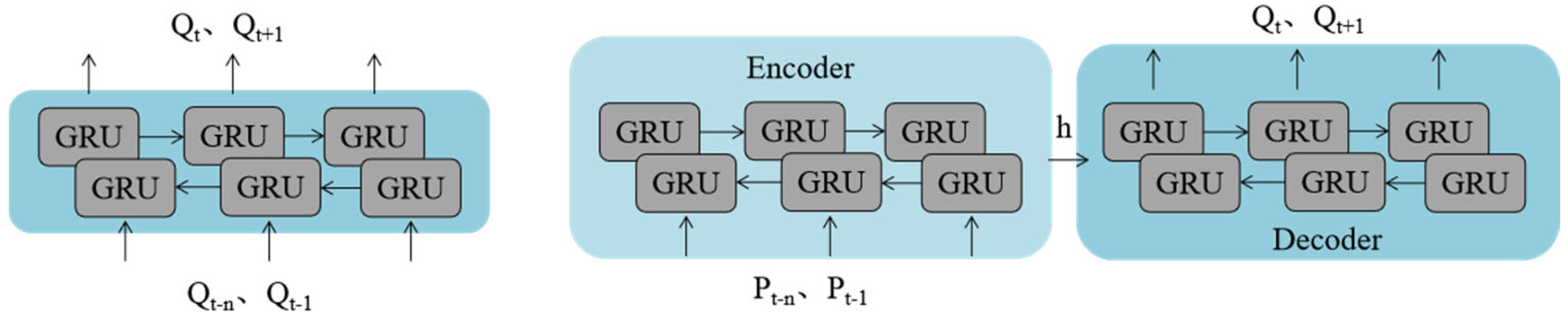
2.1. Bidirectional Gated Recurrent Unit

The bidirectional gated recurrent unit (BiGRU) constitutes an advanced multivariate time series forecasting framework built upon gated recurrent architectures. By synergistically integrating bidirectional temporal processing with sophisticated gating mechanisms, this methodology effectively captures both sequential dependencies and multivariate interactions within time-dependent datasets. As a streamlined derivative of Long Short-Term Memory (LSTM) networks, the GRU architecture achieves structural simplification through gate fusion: it consolidates the forget and input gates into a unified update gate, while merging the memory cell and hidden layer functionalities into a reset gate mechanism (Figure 1). This topological optimization results in fewer trainable parameters and lower computational complexity compared to LSTM, while demonstrating enhanced performance in capturing long-term temporal dependencies [15,16].

When processing temporal input $x_t$, the GRU cell executes three fundamental computational phases:

(a)

Enter the update gate:

$$z_t=\sigma \left[W_z\cdot \left(h_{t-1},x_t\right)\right]$$

(1)

where $W_z$ represents the weight matrix associated with the update gate and $\sigma$ represents the sigmoid activation function governing the gating operation.

(b)

Enter the reset gate:

$$r_t=\sigma \left[W_r\cdot \left(h_{t-1},x_t\right)\right]$$

(2)

where $W_r$ represents the weight matrix associated with the reset gate.

(c)

Output of GRU unit

Following the reset gate operation, a candidate hidden state ${\tilde{h}}_t$ is generated as an intermediate computational phase preceding the final hidden state update. This transitional state can be mathematically expressed as follows:

$${\tilde{h}}_t=\tanh \left[W_h\cdot \left(r_t\odot h_{t-1},x_t\right)\right]$$

(3)

where $r_t\in {[0,1]}^n$ represents the reset gate activation vector.

The final hidden state $h_t$ is computed through a gated linear interpolation between the previous hidden state $h_{t-1}$ and the candidate state ${\tilde{h}}_t$, governed by the update gate’s activation vector $z_t$:

$$h_t=\left(1-z_t\right)\odot h_{t-1}+z_t\odot {\tilde{h}}_t$$

(4)

The bidirectional GRU (BiGRU) architecture employs dual GRU subnetworks operating in opposing temporal directions: a forward GRU, processing sequential data in chronological order $(t_1\to t_n)$, and a reverse GRU analyzing the sequence in an inverted temporal context $(t_n\to t_1)$. At each timestep t, the model synthesizes temporal dependencies through hidden state concatenation:

$$h_t^{bi}=[\overrightarrow{h_t}\parallel \overleftarrow{h_t}]\in R^{2d}$$

(5)

where ${\overrightarrow{h}}_t\in R^d$ represents the hidden state derived from forward propagation; ${\overleftarrow{h}}_t\in R^d$ represents the hidden state derived from backward propagation; and $d$ represents hidden layer dimensionality.

This bidirectional processing mechanism enables comprehensive temporal feature extraction by simultaneously capturing 1. causal relationships (forward direction) and 2. retrospective patterns (reverse direction). The concatenated hidden states establish enriched contextual representations, which are particularly critical for modeling complex production dynamics in shale reservoirs where historical pressure transients and future operational constraints exhibit bidirectional temporal couplings [17].

2.2. Sequence to Sequence

While conventional machine learning approaches used for production forecasting predominantly employ recurrent neural network architectures (e.g., LSTM, GRU) with homogeneous sequence mapping (production-to-production sequence prediction), this methodology fundamentally conflicts with the physical understanding of production dynamics. From a reservoir engineering perspective, production fluctuations are principally governed by wellhead pressure transients. Mechanistically, historical pressure variations should serve as the causal driver for predicting subsequent production changes, rather than relying on autoregressive production sequence correlations.

To bridge this theoretical–practical gap, our CNN-BiGRU framework introduces three critical enhancements:

• Cross-domain sequence mapping: we implement a sequence-to-sequence (seq2seq) architecture with dedicated encoder–decoder modules.
• Physical signal embedding: we establish pressure-to-production transformation pathways through intermediate latent states (h).
• Multiscale feature fusion: w combines convolutional operations for local pressure pattern extraction with bidirectional GRU for global temporal context modeling.

As illustrated in Figure 2, the encoder processes historical pressure sequences $(P_{t-n:t})$ to generate context-rich latent representations, which the decoder subsequently translates into production forecasts $(Q_{t+1:t+m})$.This architecture explicitly captures the pressure-driven production causality while maintaining compatibility with data-driven learning paradigms.

2.3. Sliding Windows

Oil well production forecasting is inherently a multi-step forecasting problem. Before constructing the training dataset, continuous time series data must be partitioned into input–output sample pairs using a sliding window. The raw time series data contains N time steps, each with 2 features (daily well pressure and production rate), which can be represented as follows:

$$X=[x_1,x_2,\dots ,x_N]\in R^N$$

(6)

As shown in Figure 3, the raw data is partitioned into n sample pairs using a sliding window.

The input sample X_i consists of features from W consecutive time steps, starting at time step ti, and the output sample Yi contains target values for L consecutive time steps, starting from ti+W:

$$\left\{\begin{array}{l}{X}_i=[x_{ti,}{x}_{ti+1},\dots ,x_{ti+W-1}]\in R^W\\ Y_i=[y_{ti+W},y_{ti+W+1},\dots ,y_{ti+W+L-1}]\in R^L\end{array}\right.$$

(7)

After processing with a sliding window, the entire sample set can be represented as follows:

$$D={\left\{\left(X_i,Y_i\right)\right\}}_{i=1}^{N-W-L+1}$$

(8)

2.4. CNN-BiGRU Modeling

While conventional machine learning models used for production forecasting are constrained to homogeneous input architectures—typically limited to production sequence data coupled with one-dimensional static parameters through shared embedding layers—this approach fails to capture the multidimensional nature of reservoir characterization. Our CNN-BiGRU architecture addresses this critical limitation through tripartite input layer design (Figure 4), enabling the simultaneous processing of the following:

• Temporal dynamic features: production time series via BiGRU networks.
• High-dimensional static constraints: two-dimensional spatial parameters (e.g., Horizontal stress, Young’s modulus, Poisson’s ratio, etc., distributed along the depth) through CNN-based feature extraction.
• Scalar engineering parameters: one-dimensional static variables (e.g., fracturing scale, reservoir parameters, etc.) using fully connected layers.

2.5. Model Evaluation Metric

The mean squared error (MSE) is adopted as the evaluation metric for the model:

$$\mathrm{MSE}={\displaystyle \frac{1}{n}}{\displaystyle \sum _{i=1}^n{\left({\widehat{y}}_i-y_i\right)}^2}$$

(9)

In the case study, the mean relative error (MRE) is adopted as the metric to quantify the discrepancy between the model-predicted production and actual production, which provides an intuitive measure of the error proportion relative to the actual values:

$$\mathrm{MRE}={\displaystyle \frac{1}{n}}{\displaystyle \sum _{i=1}^n\left|\frac{{\widehat{y}}_i-y_i}{y_i}\right|}$$

(10)

In the equation, ${\widehat{y}}_i$ is the predicted value of the i-th sample; $y_i$ is the true value of the i-th sample; and n is the total number of samples.

3. Model Performance Discussion

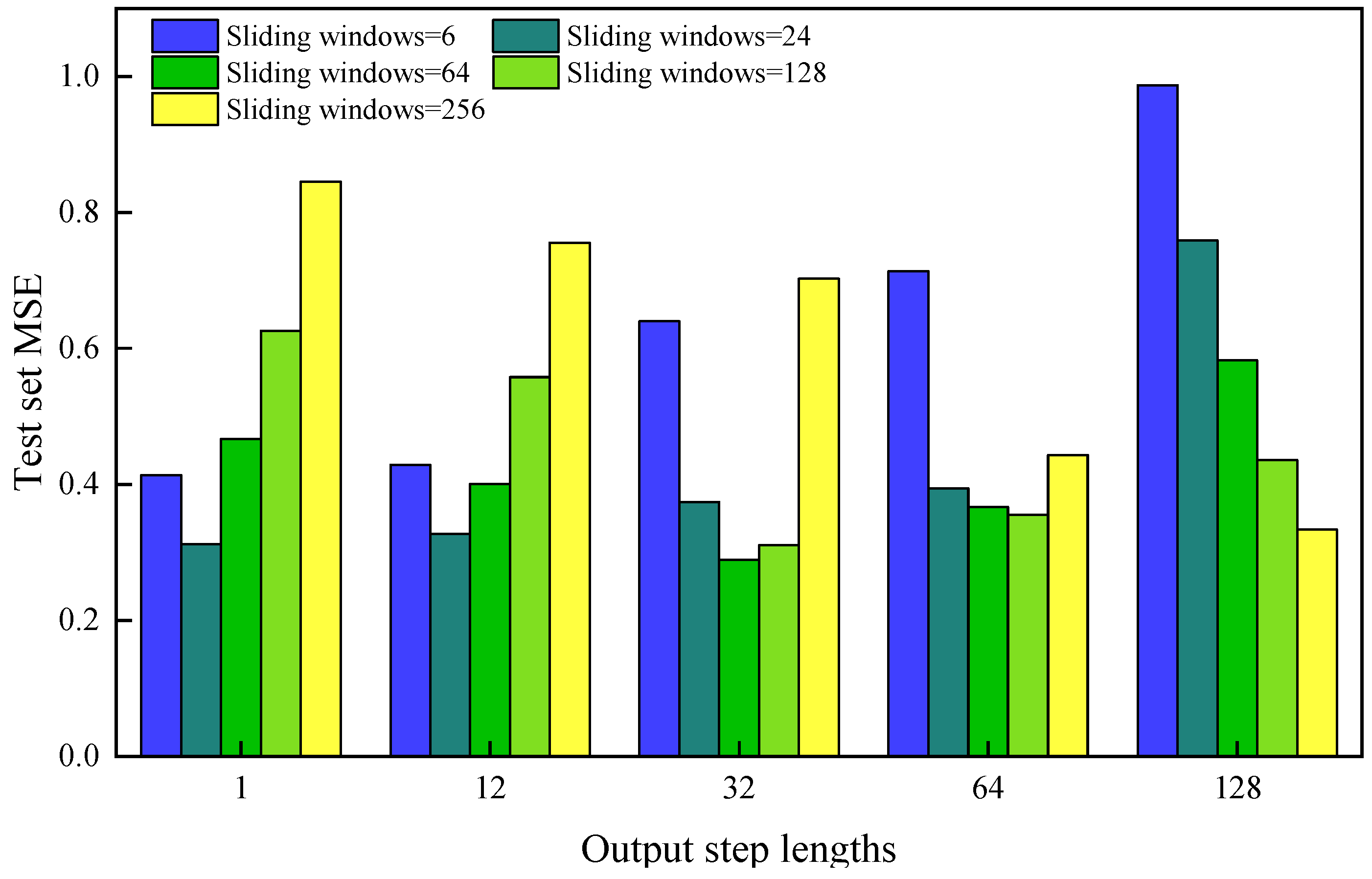
3.1. Optimization of Sliding Window and Output Step Length

The configuration of sliding window and output step length generates critical hyperparameters in production time series forecasting, exhibiting strong interdependencies through their phase–space coupling. Through systematic hyperparameter tuning, we evaluated multiple configurations:

$$\begin{array}{l}· \mathrm{Sliding} \mathrm{window} \mathrm{sizes}: \left\{6,24,64,128,256\right\}\left(\mathrm{days}\right)\\ · \mathrm{Output} \mathrm{step} \mathrm{length}: \left\{1,12,32,64,128\right\}\left(\mathrm{days}\right)\end{array}$$

As demonstrated in Figure 5, the test set mean squared error (MSE) displays distinct behavioral regimes. The model test set error increases with the increase in the prediction step when the sliding window is 6 and 24; when the sliding window is 64, 128, and 256, the results show the opposite trend. When the output step length is 1, the mean square error of the model test set with a sliding window of 24 is 0.313, which is the smallest value in all cases, indicating that too large or too small a sliding window will have an impact on the prediction performance of the model: when the sliding window is too small, the model can only consider short historical data, and cannot fully capture the long-term model of data. When the sliding window is too large, the input historical information is too miscellaneous, which increases the amount of noise or irrelevant information, leading to inaccurate predictions.

For example, comparing sliding window 24 and output step length 12 with sliding window 24 and output step length 64, Figure 6 shows the prediction of a sample in the respective model test set. The prediction effect of the first case is better, and the average relative error is 4.51%. In the second case, the average relative error is 11.74%. In the first half, the prediction results (the first 24 predicted values) fit the actual values well. However, due to the limited input information accepted by the model, the prediction results in the second half gradually deviate from the actual values.

Finally, according to the prediction results of the model, the optimal output step length under different sliding windows is counted, as shown in

Table 1. Optimal output step length under different sliding windows.

Sliding Windows Size	The Best Output Step Length	Test Set MSE
6	1	0.431
24	1	0.313
64	32	0.289
128	64	0.311
256	128	0.342

.

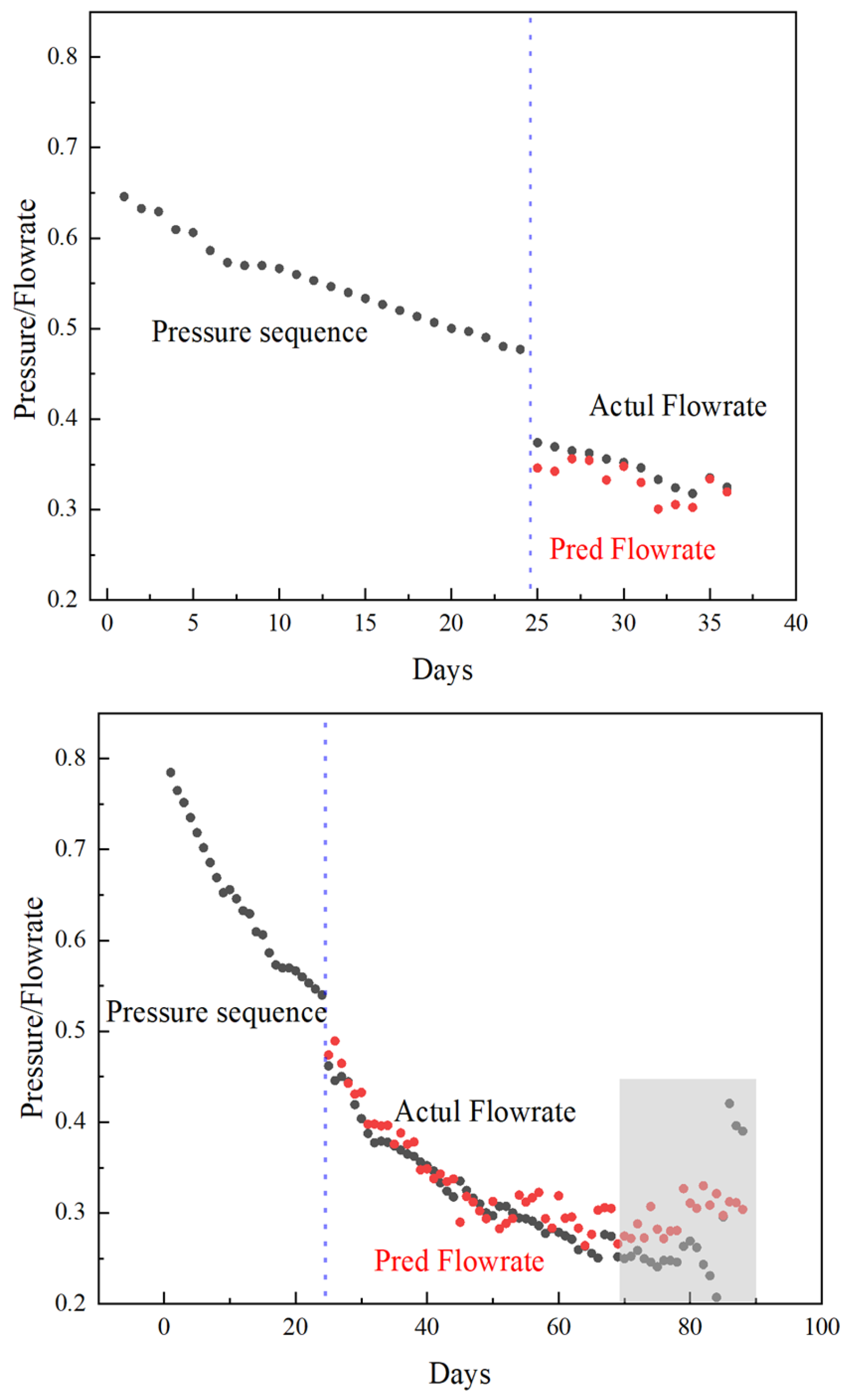
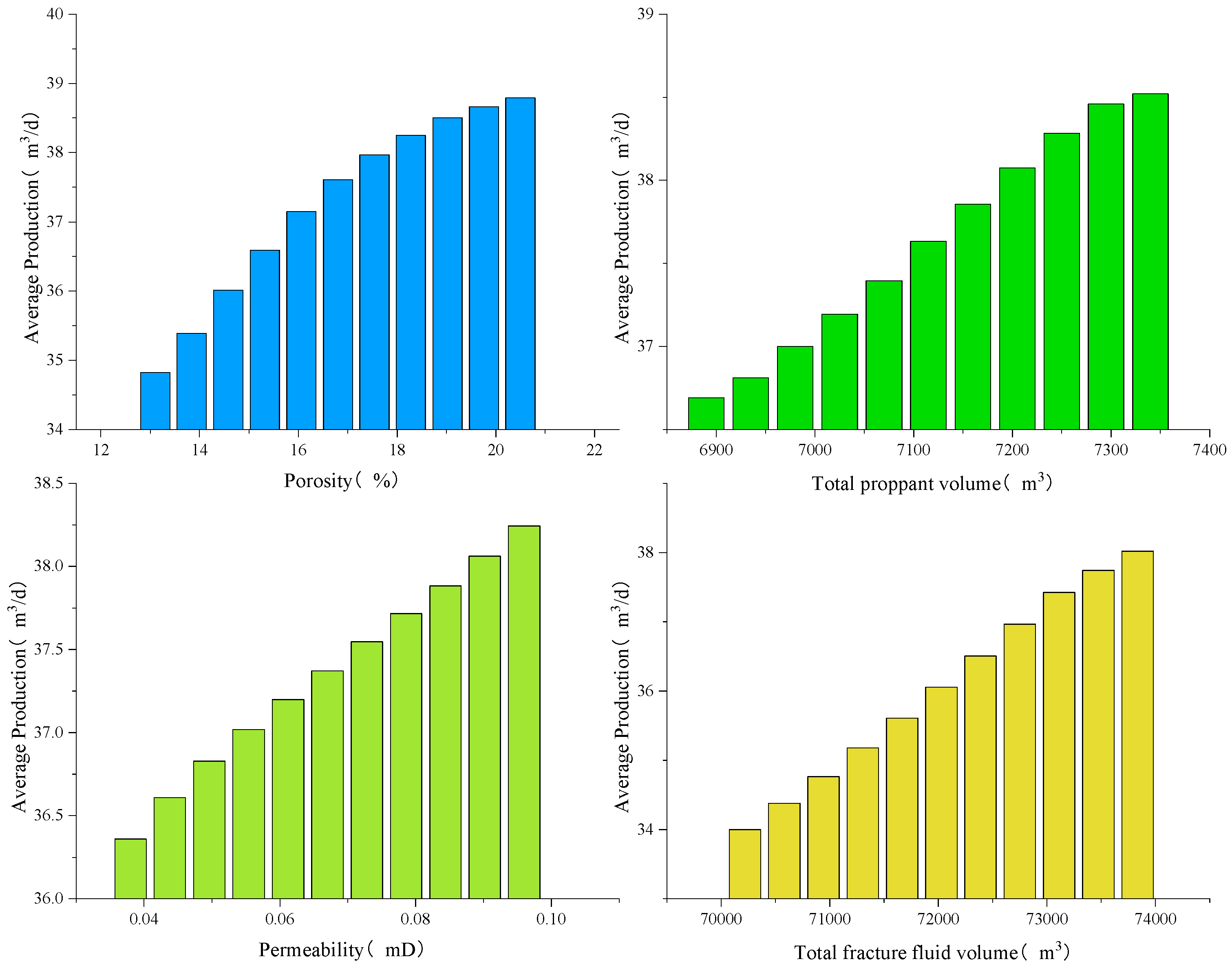
3.2. Reliability Assessment

To evaluate the physical plausibility of prediction outcomes and decode the model’s decision-making mechanics, we conducted controlled-variable sensitivity analysis on the CNN-BiGRU architecture. The experimental protocol comprised the following components:

• Parameter space discretization: uniform sampling of 11 points across normalized ranges for key features.

$$\begin{array}{l}· \mathrm{Geological} \mathrm{parameters}: \mathrm{Porosity}(\varphi ), \mathrm{Permeability}(\mathrm{k})\\ ·{ \mathrm{Completion} \mathrm{parameters}: \mathrm{Total} \mathrm{proppant} \mathrm{volume} (\mathrm{V}}_p{), \mathrm{Total} \mathrm{fracturing} \mathrm{fluid} \mathrm{volume} (\mathrm{V}}_f)\end{array}$$

• Univariate perturbation: holding other variables at baseline values while systematically varying target parameters through discretized levels.
• Production prediction: aggregating predicted production across test set samples through ensemble averaging.

$${\widehat{Q}}_i={\displaystyle \frac{1}{N}}{\displaystyle \sum _{j=1}^N{f}_{CNN-BiGRU}(x_j^{(i)})}$$

(11)

where $x_j^{(i)}$ denotes the j-th sample with a perturbed i-th feature.

As evidenced in Figure 7, the univariate response curves demonstrate first-principle consistency:

• Geological controls: production scales positively with ϕ (storage capacity) and k (fluid conductivity), aligning with Darcy’s law and capillary pressure theory.
• Completion efficiency: hyperbolic growth patterns emerge for $V_p$ and $V_f$, reflecting fracture conductivity enhancement and drainage volume expansion mechanisms.

This parametric sensitivity analysis confirms the model’s capability to preserve the causality constraints inherent in multiphase flow dynamics, while simultaneously processing temporal production signatures through BiGRU, processing spatial heterogeneity via CNN, and processing scalar parameters through dense layers. The concordance between data-driven predictions and petrophysical fundamentals substantiates the model’s reliability for field-scale decision support in unconventional resource development [18].

3.3. Input Feature Analysis

The impact of diverse input features on model predictions is systematically evaluated through ablation experiments. First, input characteristics are categorized into three distinct physical domains (

Table 2. Classification of input features.

Geological Features	Engineering Features	Time Series
Penetration rate (%)	Vertical depth (m)	Wellhead pressure (MPa)
Porosity (%)	Length of horizontal section (m)
Permeability (mD)	Fracturing stages
Oil saturation (%)	Fracturing clusters
“Dessert” thickness (m)	Fracturing fluid volume (m3)
Two-dimensional stress difference (MPa)	Proppant volume (m3)
Young’s modulus (GPa)
Poisson’s ratio

):

• Geological features: petrophysical parameters derived from logging interpretation (e.g., porosity, permeability).
• Engineering features: completion and hydraulic fracturing parameters (e.g., proppant volume, stage spacing).
• Temporal features: wellhead pressure time series data.

Subsequently, each feature category is individually fed into the CNN-BiGRU model to isolate its predictive contribution.

As demonstrated in Figure 8, Figure 9 and Figure 10, the temporal features exhibit the strongest predictive influence with the lowest test set MSE (0.46), confirming the critical time-dependent coupling between wellhead pressure dynamics and wellhead production regimes. Geological features show moderate predictive capability (test MSE 1.09), outperforming engineering features (test MSE 1.29) yet still deviating significantly from actual measurements. This discrepancy arises from insufficient physical constraints in static feature representations and temporal invariance limitations evident in the near-constant predictions.

Fundamentally, the model deciphers distinct physical information through the following features:

• Geological parameters encode reservoir flow capacity, heterogeneity, and fracture network geometry.
• Engineering parameters reflect stimulation intensity and fracture conductivity potential.
• Temporal features capture transient flow behavior and pressure propagation.

The CNN-BiGRU architecture synergistically integrates these components:

• Geological/engineering features constrain production trend baselines.
• Temporal features resolve short-term production fluctuations.
• Combined inputs establish multiphysics-constrained predictions.

4. Case Study

4.1. Dataset Construction

Production data from eight horizontal shale oil wells in Field A were acquired for this study. The scalar static parameters were obtained from stage-specific fracturing designs and field development plans of the subject wells, comprising the following components:

• Geological attributes: length of horizontal section, penetration rate, porosity, permeability, oil saturation, “Dessert” thickness, Young’s modulus, Poisson’s ratio.
• Completion parameters: number of stages, number of clusters, proppant loading intensity, fluid volume per stage, cluster spacing.

Recognizing the limitations of univariate static features in establishing comprehensive production mapping relationships, we incorporated depth-dependent geomechanical profiles as two-dimensional static inputs. Using the JewelSuite2018 GeoMechanics simulator, we calculated true vertical depth (TVD)-correlated horizontal stress gradients, Young’s modulus distributions, and Poisson’s ratio variations. These parameters characterize fracture geometry evolution during stimulation—critical for capturing stimulated reservoir volume (SRV) dynamics.

Temporal features included daily measurements of the following parameters:

• The wellhead pressure sequence—this sequence serves as the input sequence (production sequence) for the model.
• The oil production sequence—this sequence serves as the output sequence (target sequence) of the model.

The dataset underwent Z-score normalization to mitigate scale discrepancies among heterogeneous parameters:

$$z={\displaystyle \frac{x-\mu }{\Sigma }}$$

(12)

where $\mu$ and $\Sigma$ denote feature-specific means and standard deviations, respectively. The normalized parameter distributions and transformation metrics are cataloged in

Table 3. Sample set feature statistics.

Feature Type	Feature Name	Range	Average	Standard Deviation
1D static characteristics	Vertical depth/m	3561.0~3601.2	3582.7	15.1
	Length of horizontal section/m	1800.0~1812.6	1698.7	254.1
	Penetration rate/%	86.8~99.4	91.6	5.4
	Porosity/%	13.1~20.5	16.5	2.5
	Permeability/mD	0.039~0.096	0.1	0.02
	Oil saturation/%	89.8~93.1	92.1	1.2
	“Dessert” thickness/m	797.0~1675.5	1408.1	311.9
	Number of stages	37.0~40.0	39.0	1.1
	Number of clusters	289.0~307.0	299.8	6.1
	Fracturing fluid volume/m3	70,219.1~73,836.4	72,241.8	1215.8
	Proppant volume/m3	6890.2~7340.5	7166.6	152.6
2D static characteristics	Depth/m	3561.2~3695.4	3628.5	33.04
	Two-dimensional stress difference/MPa	16.8~17.8	27.3	0.2
	Young’s modulus/GPa	12.8~43.8	28.5	7.8
	Poisson’s ratio	0.2~0.3	0.2	0.01
Production sequence	Wellhead pressure/MPa	0.1~29.3	4.2	5.9
Target sequence	Daily production/m3	5.8~117.9	38.7	23.5

.

4.2. Superparametric Optimization

The neural architecture was implemented using TensorFlow 2.13 with Keras 2.13.1 API integration. The model’s optimization framework employed the following components:

• Objective function: mean squared error (MSE) as both a loss metric and an evaluation criterion.
• Data partitioning: stratified 70:20:10 training–validation–test split ratio.

Bayesian optimization with Gaussian processes was conducted over the hyperparameter space:

• Activation functions: ReLU, Sigmoid, Tanh (input layer selection)
• Convolutional architecture:

Filter count: 3 to 21

Kernel size: 3 × 1 to 6 × 1

• BiGRU configuration:

Encoder/decoder hidden units: 32 × 2 to 128 × 2 neurons per layer

Layer depth: 1–4 (constrained by computational cost and accuracy, Figure 11)

As an example, Figure 11 illustrates the model’s computational workflow with a sliding window size of 6. The input tensor dimensions are configured as follows (Figure 12):

• 1D static features: processed as 3D tensor (3158, 6, 11)
• 2D static features: structured as 4D tensor (3158, 6, 11, 4)
• Temporal features: formatted as 3D tensor (3158, 6, 1)

The feature extraction pipelines operate as follows:

• 1D feature processing:

Input shape: (6, 11)

Transformation: fully connected layer with dimensional preservation

Output shape: (6, 11)

• 2D feature processing:

Input shape: (6, 11, 4)

Convolutional layer: 3 × 1 kernels with stride = 1 → output shape: (6, 9, 11)

Flattening: merged axis 2–3 → final output shape: (6, 99)

• Temporal feature processing:

Input shape: (6, 1)

Transformation: fully connected layer with feature expansion

Output shape: (6, 11)

The extracted features are concatenated along the temporal dimension (axis = 2), forming a fused tensor of shape (6, 121). This composite representation sequentially propagates through the BiGRU encoder–decoder architecture to generate final production predictions.

The model employs a batch size of 32 with 100 training iterations. As depicted in Figure 13, both training and validation loss values exhibit a steady decreasing trend before converging to stability post 100 epochs. The optimal hyperparameter configuration derived from this convergence analysis is systematically presented in

Table 4. Optimization results of model parameters.

Superparameter Type		Activation Function	Superparametric Optimization Value
Input layer	1D static characteristics	ReLU	/	/
	2D static characteristics	ReLU	Convolution kernel size	3
			Number of convolution kernels	11
	Production series	ReLU	Convolution kernel size	3
			Number of convolution kernels	11
Middle layer	Encoder	Sigmoid	Number of neurons	64 × 2
		Tanh
	Decoder	Sigmoid	Number of neurons	64 × 2
		Tanh

.

The model’s test set predictions under optimized hyperparameters are visualized in Figure 14. While sparse outliers exist, the model achieves strong concordance with the majority of samples clustered within the (−1, 1) normalized range. The test set MSE of 0.46 confirms that there was effective generalization without evidence of overfitting. Furthermore, the prediction residuals demonstrate approximately uniform distribution along the zero mean baseline (mean residual = 0.004), quantitatively validating the model’s systematic alignment between predicted and observed production values.

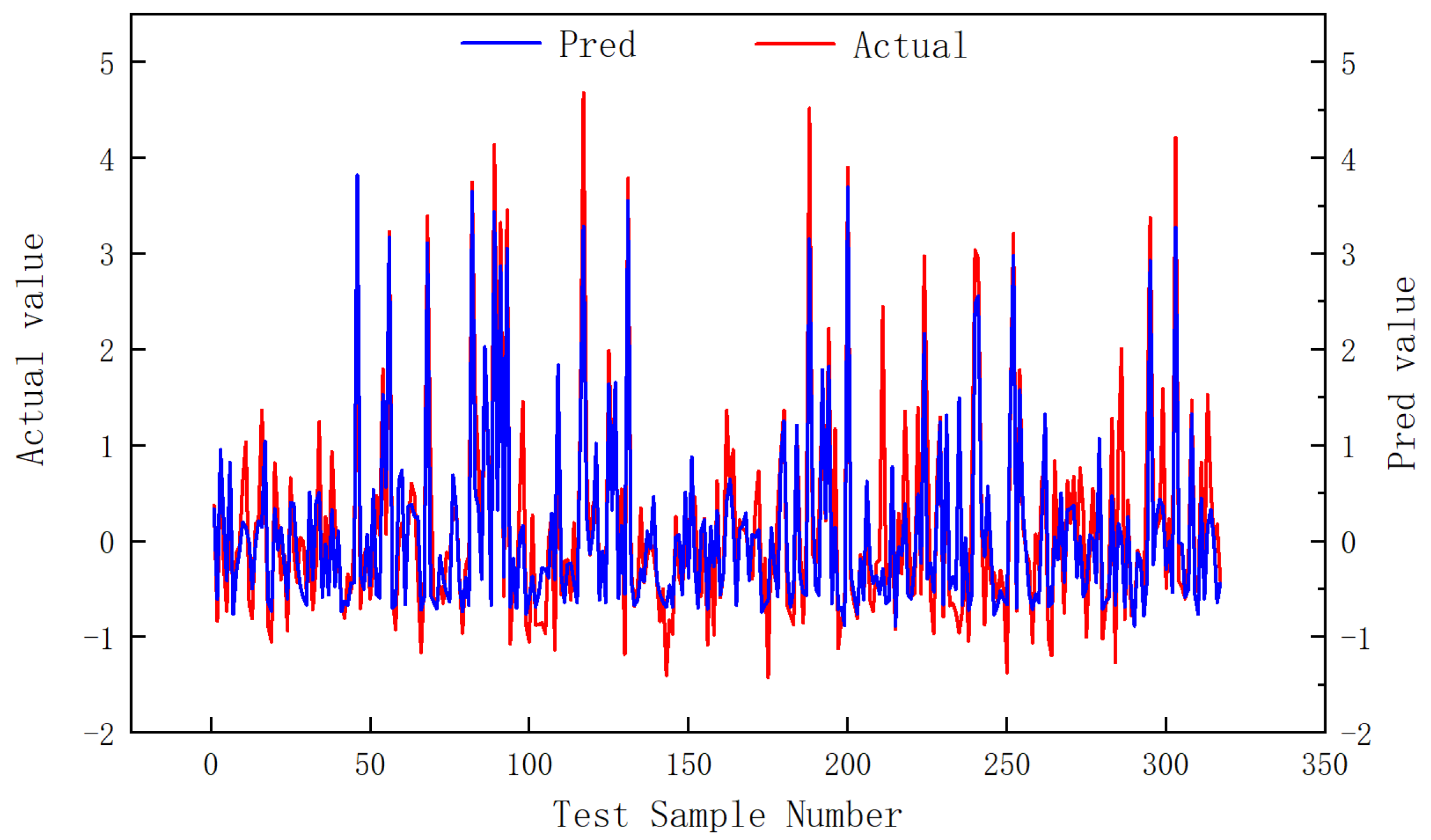
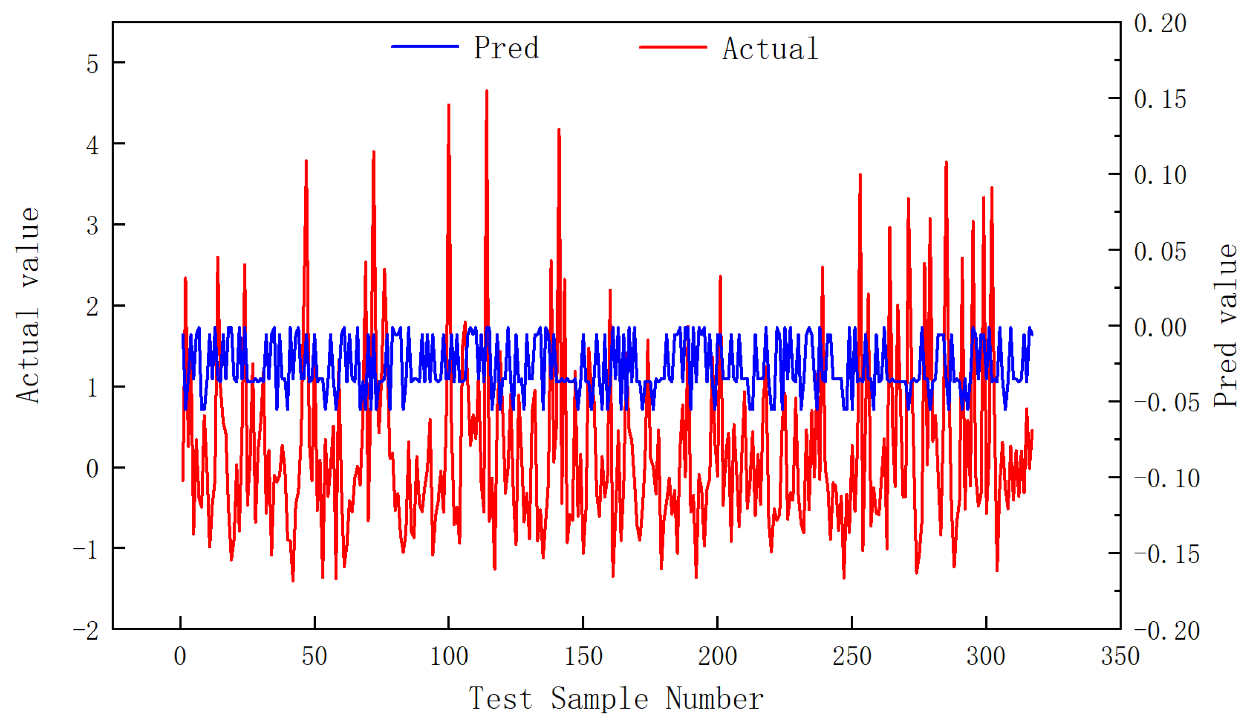
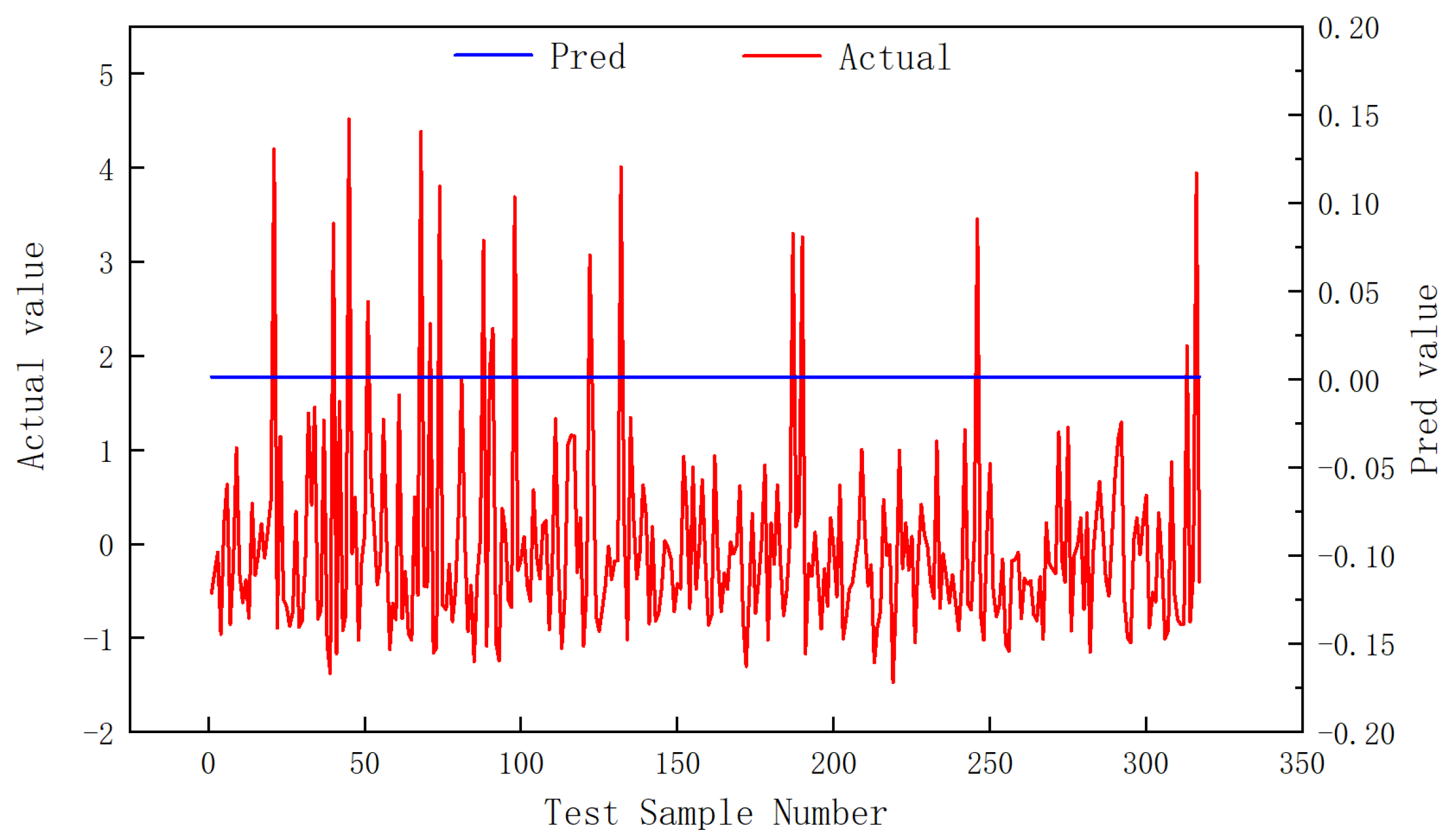
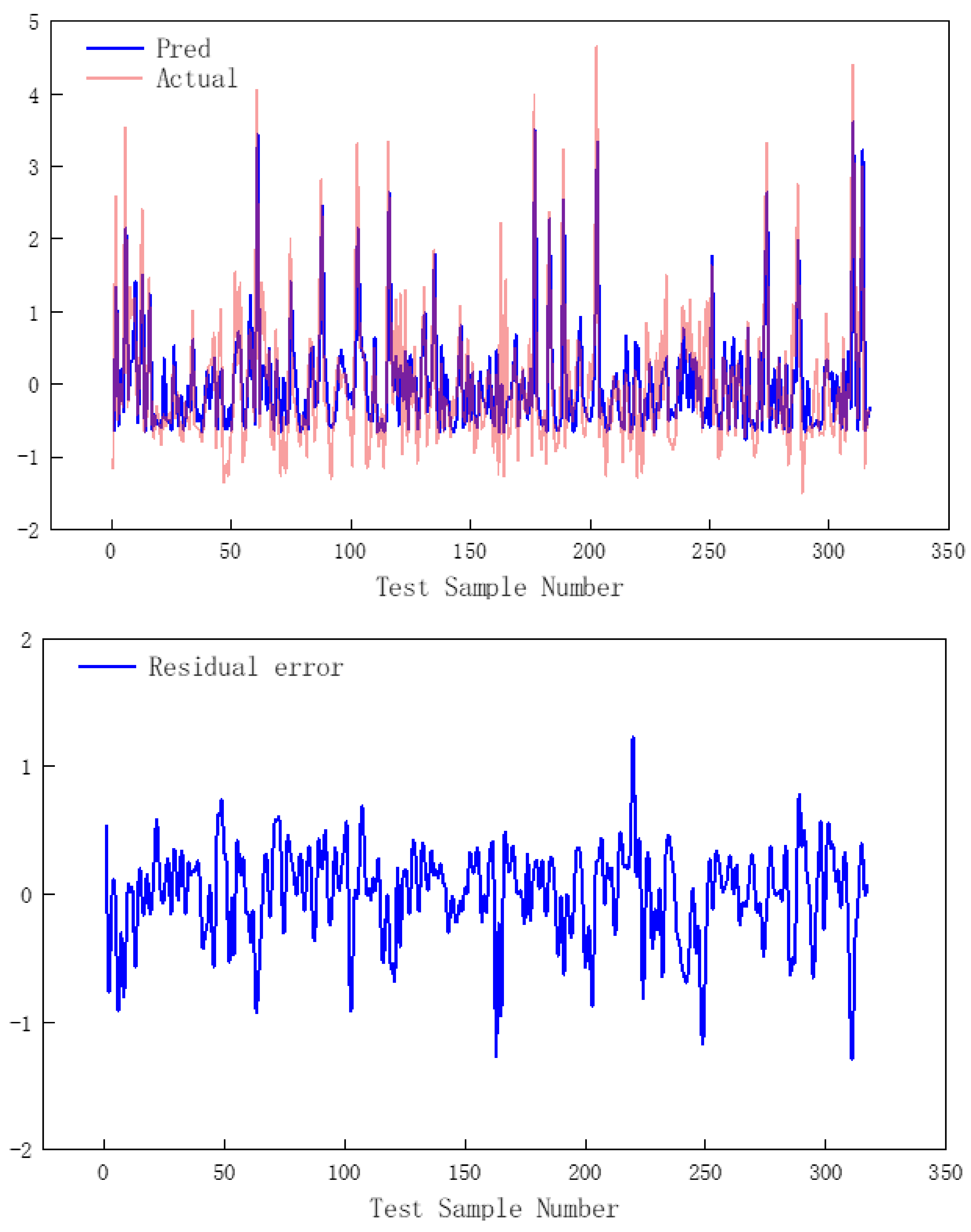
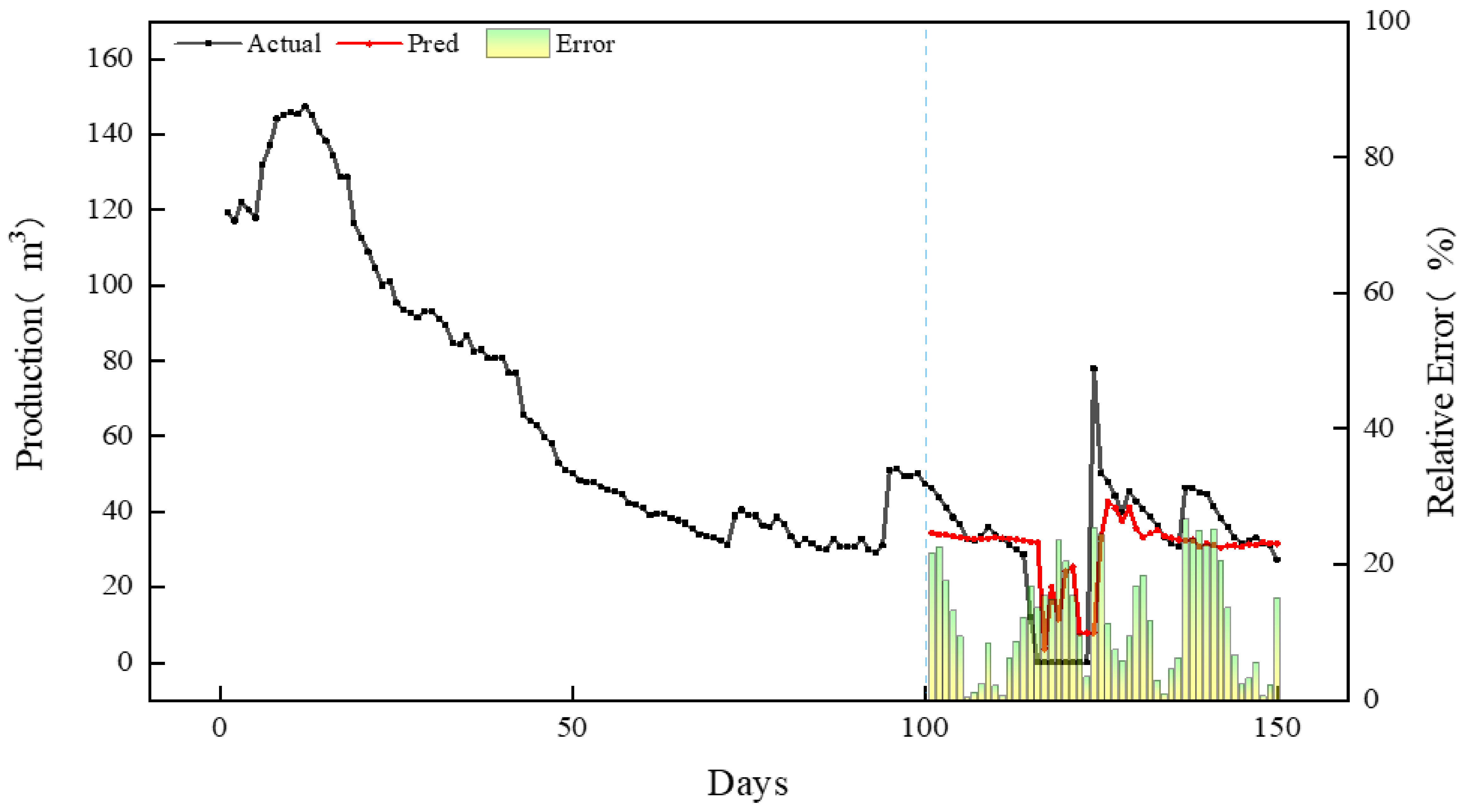
4.3. CNN-BiGRU Model Application

Well A1 features a 1800 m horizontal section with reservoir permeability of 0.077 mD and 303-stage fracturing clusters. During the initial 100 production days, daily oil production exhibited a decline from 98 m³ to 40 m³. To optimize the production strategy, we configured the sliding window to 100 days and forecast horizon to 50 days based on the well’s petrophysical profile. The model’s 50-day production forecast (Figure 15) demonstrates strong concordance with actual decline trends, achieving a mean relative error (MRE) of 16.11% between predicted and measured production rates.

5. Conclusions

(1)

The CNN-BiGRU productivity prediction framework was successfully implemented on the TensorFlow deep learning platform. Systematic analysis revealed optimal temporal context configurations: sliding window—6/24/128/256 days; corresponding optimal forecast horizons—1/1/32/64/128 days.

(2)

Controlled-variable experiments demonstrated physical consistency with established reservoir engineering principles. The model effectively reconciles geological constraints, completion impacts, temporal dynamics.

(3)

Feature ablation studies quantified distinct physical roles. The results show that geological and engineering characteristics are responsible for constraining the overall trends in production, while time series characteristics are used to study the subtle fluctuations during production, which can comprehensively constrain production.

(4)

The hyperparameters of the model were optimized based on Bayesian optimization method. The results showed that the number of BiGRU neurons was 64 × 2, the number of CNN convolution cores was 11, and the size of convolution cores was 3. The mean square error of the model test set is 0.46 and the average residual error is 0.004, indicating that the model can be used for learning tasks between different sequences. In addition, the application results of the model show that the average relative error of the actual production prediction is 16.11%, and the prediction accuracy is high.

References

1. Guo, J.; Ren, W.; Zeng, F.; Luo, Y.; Li, Y.; Du, X. Unconventional oil and gas well fracturing parameter intelligent optimization: Research progress and future development prospects. Pet. Drill. Tech. 2023, 51, 1–7. [Google Scholar]
2. Li, Y.; Zhao, Q.; Lyu, Q.; Xue, Z.; Cao, X.; Liu, Z. Evaluation technology and practice of continental shale oil development in China. Pet. Explor. Dev. 2022, 49, 955–964. [Google Scholar] [CrossRef]
3. Li, Y. Study on Main Control Factors and Production Prediction of Single Well Production of Coalbed Methane Based on Machine Learning. Master’s Thesis, China University of Petroleum, Beijing, China, 2017. [Google Scholar]
4. Clar, F.H.; Monaco, A. Data-driven approach to optimize stimulation design in Eagle Ford formation. In Proceedings of the Unconventional Resources Technology Conference, Denver, CO, USA, 22–24 July 2019. [Google Scholar]
5. Kyungbook, L.; Jungtek, L.; Daeung, Y.; Hyungsik, J. Prediction of Shale-Gas Production at Duvernay Formation Using Deep-Learning Algorithm. SPE J. 2019, 24, 2423–2437. [Google Scholar]
6. Pan, Y.; Wang, Y.; Che, M.; Liao, R.; Zheng, H. Post-fracturing production prediction and fracturing parameter optimization of horizontal wells based on grey relational projection random forest algorithm. J. Xi’an Shiyou Univ. Nat. Sci. Ed. 2021, 36, 71–76. [Google Scholar]
7. Wan, X.; Zou, Y.; Wang, J.; Wang, W. Prediction of Shale Oil Production Based on Prophet Algorithm. In Proceedings of the 3rd International Conference on Polymer Synthesis and Application, Nanjing, China, 23–25 July 2021. [Google Scholar]
8. Huang, C.; Tian, L.; Wang, H.; Wang, J.; Jiang, L. A Single Well Production Forecasting Model of Reservoir Based on Conditional Generative Adversarial Net. Chin. J. Comput. Phys. 2022, 39, 465–478. [Google Scholar]
9. Zhang, D.; Zhang, L.; Tang, H.; Zhao, Y. Fully coupled fluid-solid productivity numerical simulation of multistage fractured horizontal well in tight oil reservoirs. Pet. Explor. Dev. 2022, 49, 338–347. [Google Scholar] [CrossRef]
10. Ozkan, E.; Brown, M.L.; Raghavan, R.; Kazemi, H. Comparison of Fractured-Horizontal-Well Performance in Tight Sand and Shale Reservoirs. SPE Reserv. Eval. Eng. 2011, 14, 248–259. [Google Scholar] [CrossRef]
11. Song, X.Y.; Liu, Y.T.; Ma, J.; Wang, J.Q.; Kong, X.M.; Ren, X.N. Productivity forecast based on support vector machine optimized by grey wolf optimizer. Lithol. Reserv. 2020, 32, 134–140. [Google Scholar]
12. Hu, Q.; Liu, C.; Zhang, J.; Cui, X.; Wang, Q.; Li, J.; He, S. Machine learning-based coalbed methane well production prediction and fracturing parameter optimization. Pet. Reserv. Eval. Dev. 2025, 15, 266–273. [Google Scholar]
13. Sutskever, I.; Vinyals, O.; Le, Q.V. Sequence to Sequence Learning with Neural Networks. arXiv 2014, arXiv:1409.3215. [Google Scholar]
14. Cho, K.; van Merrienboer, B.; Gulcehre, C.; Bahdanau, D.; Bougares, F.; Schwenk, H.; Bengio, Y. Learning Phrase Representations using RNN Encoder-Decoder for Statistical Machine Translation. arXiv 2014, arXiv:1406.1078. [Google Scholar]
15. Lecun, Y.; Bottou, L. Gradient-based learning applied to document recognition. Proc. IEEE 1998, 86, 2278–2324. [Google Scholar] [CrossRef]
16. Liu, J.; Yang, Y.; Lv, S.; Wang, J.; Chen, H. Attention-based BiGRU-CNN for Chinese question classification. J. Ambient. Intell. Humaniz. Comput. 2019, 1, 1–12. [Google Scholar] [CrossRef]
17. Shalabi, L.; Shaaban, Z.; Kasasbeh, B. Data mining: A preprocessing engine. J. Comput. Sci. 2006, 2, 735–739. [Google Scholar] [CrossRef]
18. Huang, J. Modeling and Application of Horizontal Well Production Prediction Based on Machine Learning. Ph.D. Thesis, China University of Geosciences, Beijing, China, 2020. [Google Scholar]
Figure 1. Schematic diagram of gate control cycle unit.
Energies 18 02523 g001
Figure 2. Traditional GRU structure (left); seq2seq structure (right).
Energies 18 02523 g002
Figure 3. Time series data is processed using a sliding window method.
Energies 18 02523 g003
Figure 4. CNN-BiGRU model structure.
Energies 18 02523 g004
Figure 5. Model test set MSE under different sliding windows and output step lengths.
Energies 18 02523 g005
Figure 6. Comparison of prediction results under different sliding windows and output step lengths.
Energies 18 02523 g006
Figure 7. Influence of different factors on production.
Energies 18 02523 g007
Figure 8. Test set prediction results for input time series features.
Energies 18 02523 g008
Figure 9. Test set prediction results for input geological features.
Energies 18 02523 g009
Figure 10. Test set prediction results for input engineering features.
Energies 18 02523 g010
Figure 11. Training time cost and MSE with different number of layers.
Energies 18 02523 g011
Figure 12. CNN-BiGRU model workflow.
Energies 18 02523 g012
Figure 13. CNN-BiGRU model loss error changes.
Energies 18 02523 g013
Figure 14. Test set prediction results.
Energies 18 02523 g014
Figure 15. Prediction results of CNN-BiGRU model.
Energies 18 02523 g015