
Advances in Modeling and Optimization of Intelligent Power Systems Integrating Renewable Energy in the Industrial Sector: A Multi-Perspective Review


Abstract
1. Introduction
- The widespread adoption and development of industrial microgrids remain in the exploratory stage, without comprehensive standardized frameworks for their fundamental architecture and operational patterns. This review describes the fundamental architecture, configuration, and operational characteristics of industrial microgrids, providing theoretical support for their programming and application.
- The volatility and complexity of renewable energy and industrial loads restrict the accuracy and adaptability of traditional source-load forecasting methods, hurting microgrids’ economical and reasonable scheduling. This review examines multiple intelligent modeling strategies for source-load forecasting to provide a range of alternatives for increasing the quality of microgrid scheduling decisions.
- The existing microgrid scheduling optimization methods exhibit distinct advantages and disadvantages, making them inadequate for the efficient operation of complex industrial scenarios. This review summarizes general modeling approaches for industrial microgrid scheduling, laying the foundation for the intelligent management of industrial microgrids.
2. Review Methodology and Strategy
2.1. Scope of Literature Search
2.2. Criteria of Literature Selection
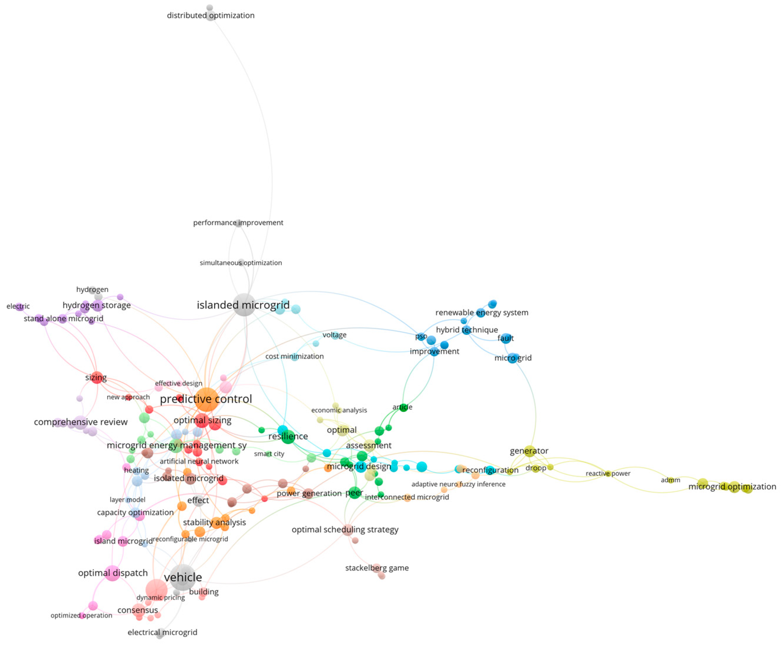
2.3. Review Methodology
3. Basic Concept and System Architecture of Smart Microgrid
3.1. Fundamental Concepts and Response Functions of Smart Microgrids
3.1.1. Smart Microgrid
3.1.2. Demand-Side Flexibility
3.2. System Architecture of Microgrid
3.2.1. Basic Architecture of Microgrid
- (1)
- Physical component layer
- (2)
- Communication layer
- (3)
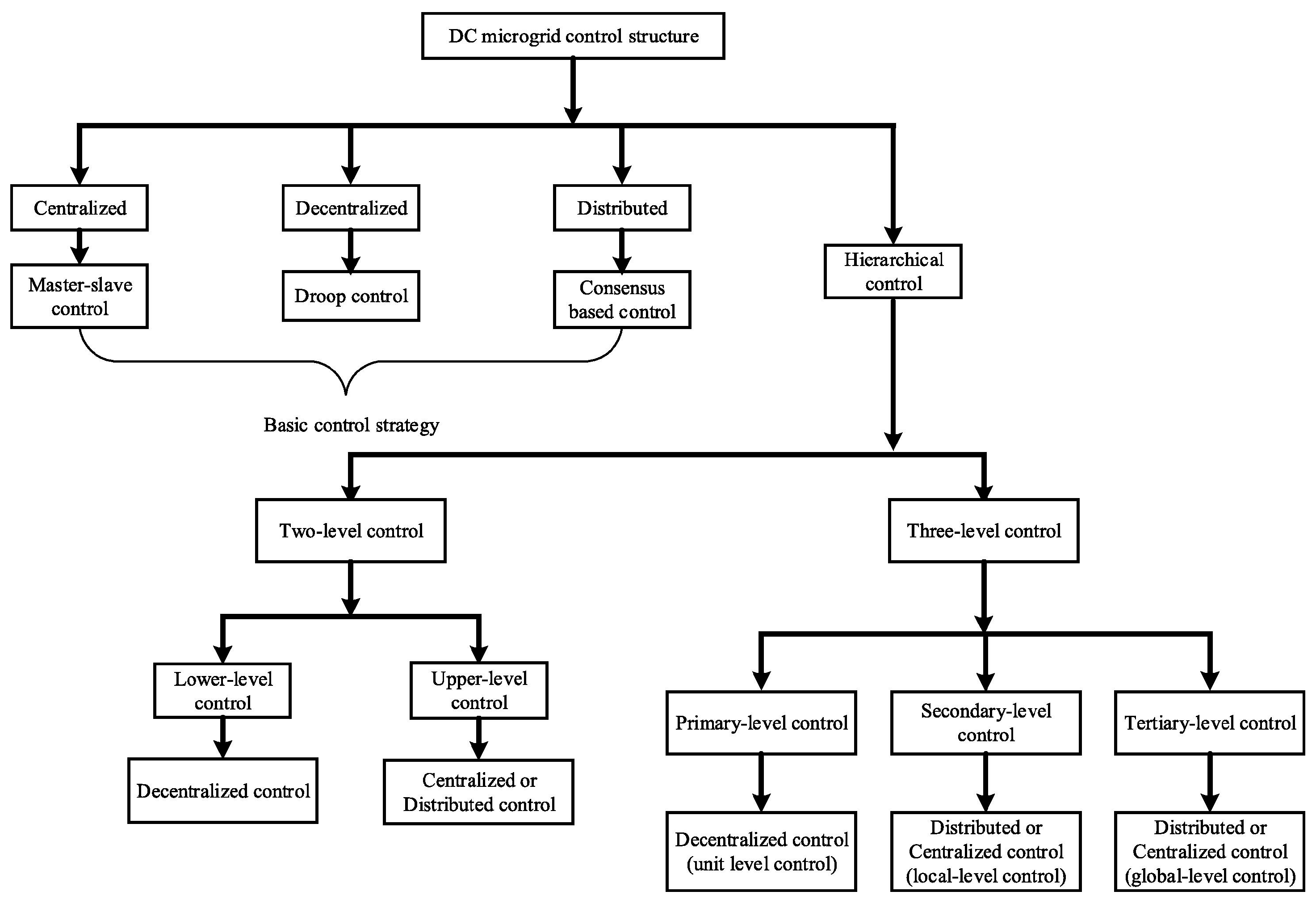
- Control layer
3.2.2. Power Supply Modes of Microgrids
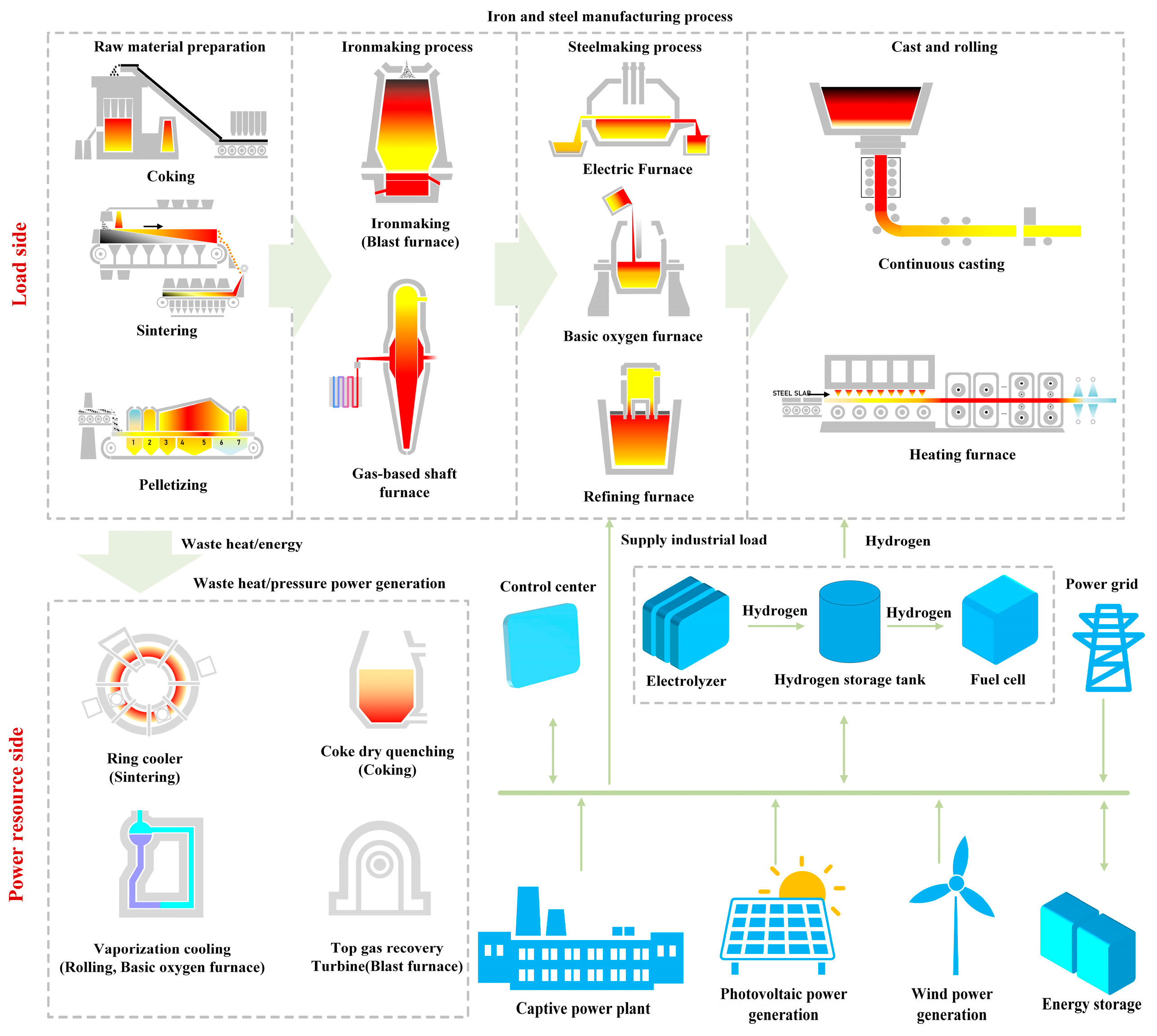
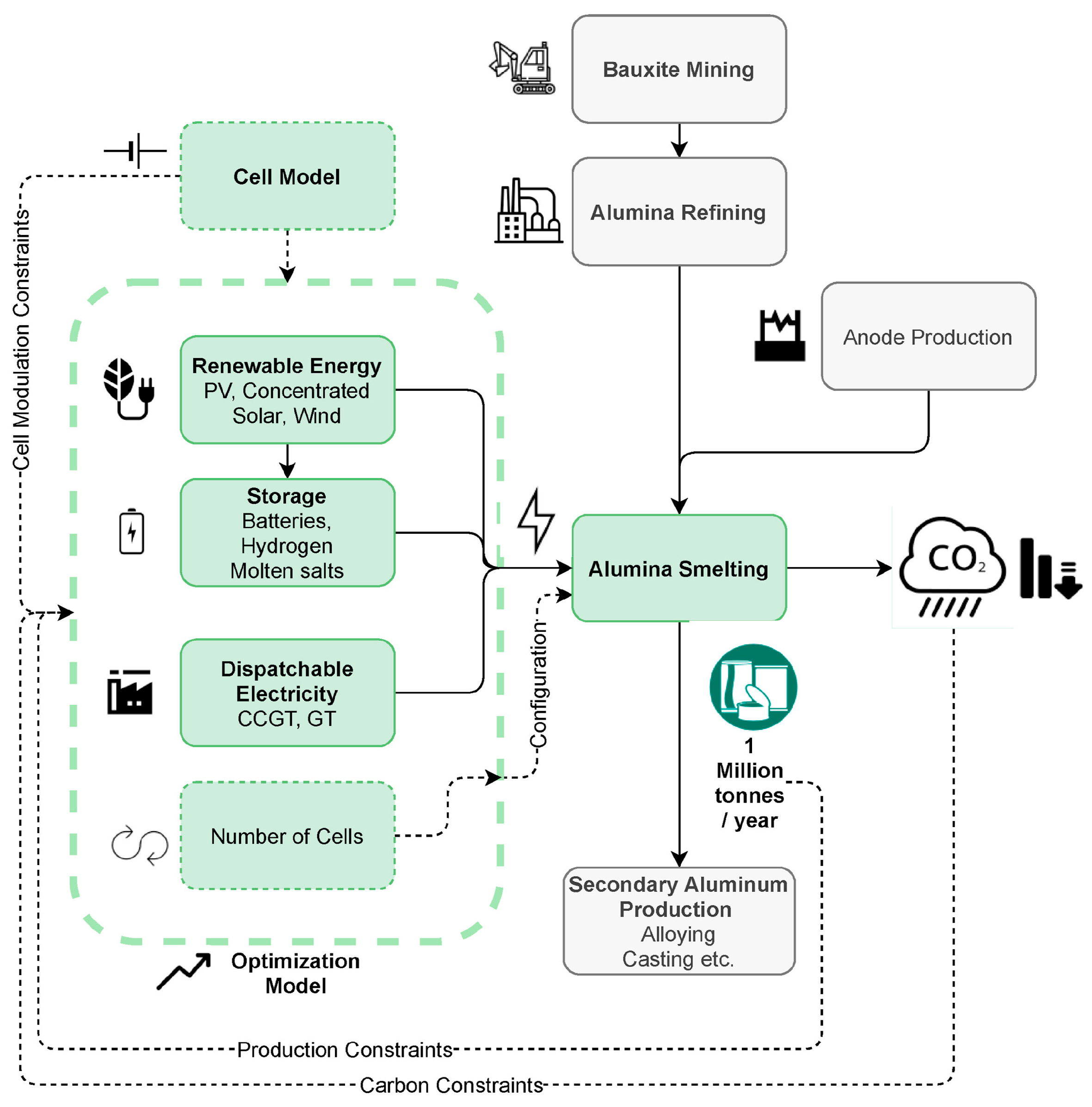
3.2.3. Flexible Microgrids Integrating Industrial Loads
4. Modeling Technologies for Intelligent Prediction
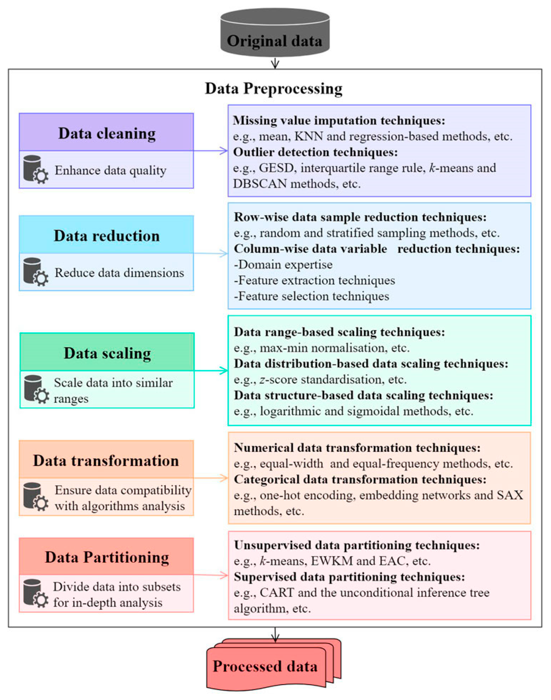
4.1. Raw Data Processing
4.1.1. Data Cleaning
4.1.2. Data Reduction
4.2. Prediction Strategy Selection
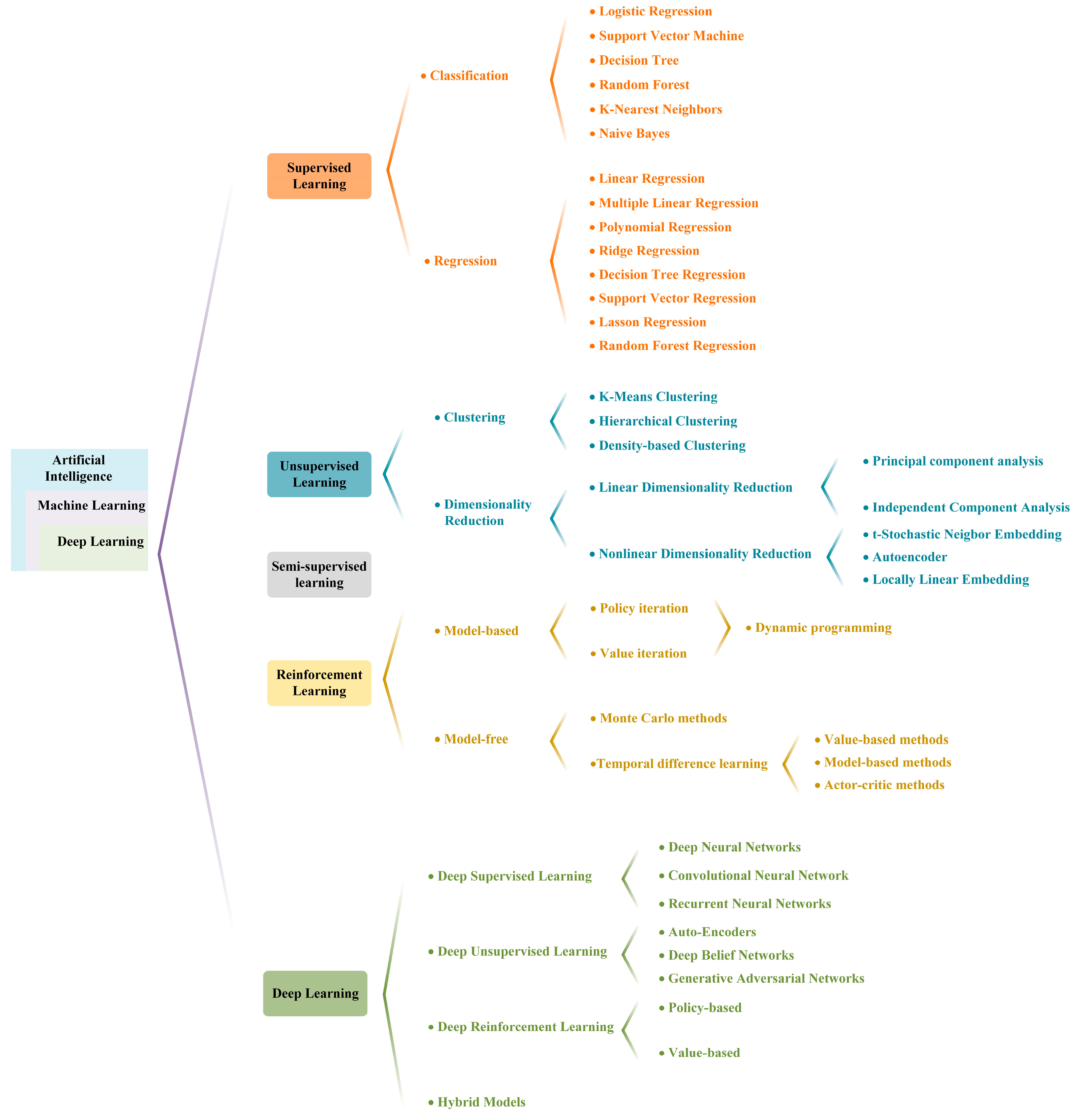
4.3. Prediction Model
4.3.1. Supervised Learning
4.3.2. Unsupervised Learning
4.3.3. Reinforcement Learning
4.3.4. Deep Learning
4.4. Model Assessment
5. Modeling Technologies for Intelligent Optimization and Scheduling
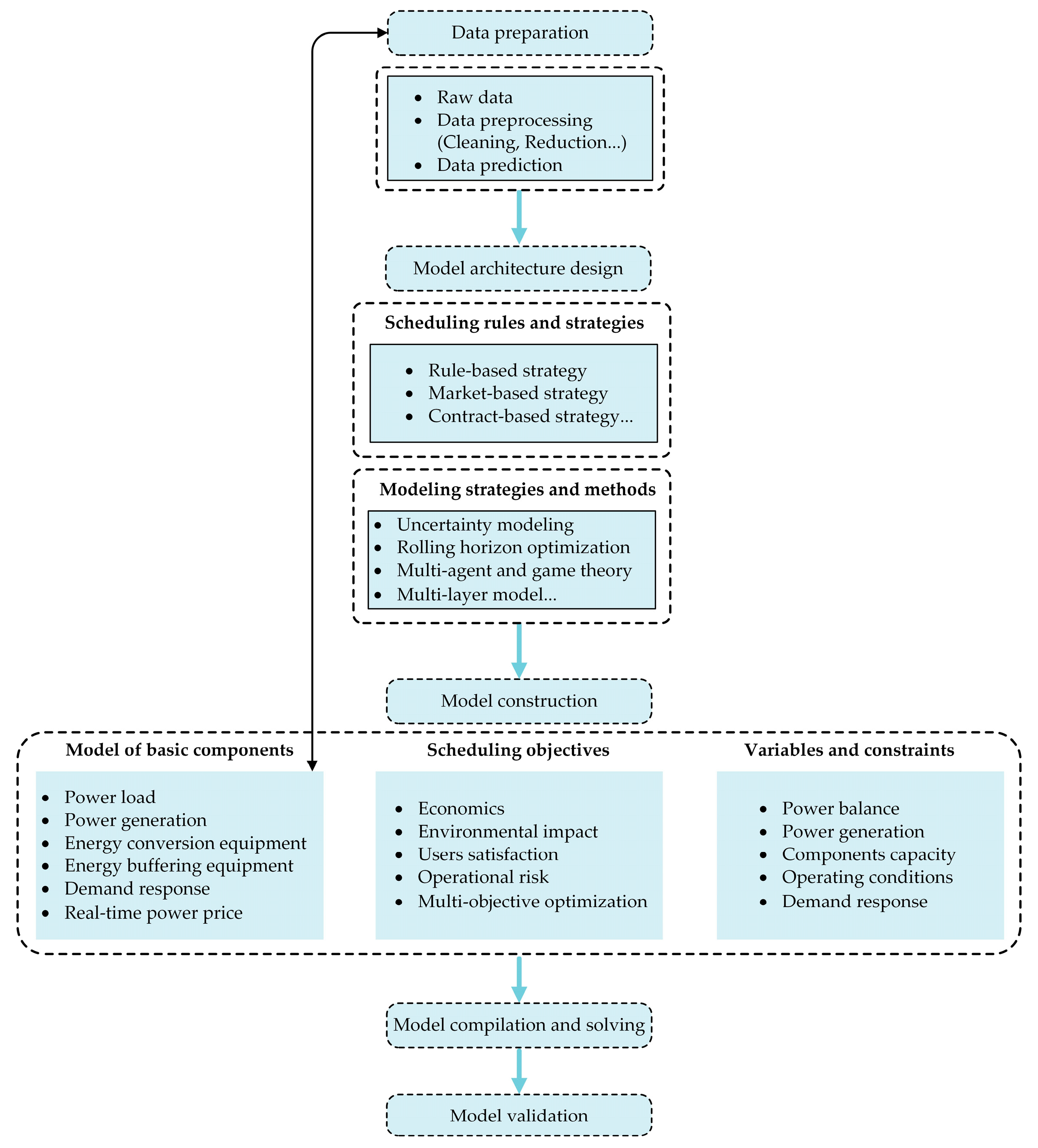
5.1. Model of Basic Components in Microgrids
- (1)
- Modeling of load
- (2)
- Modeling of power-generation equipment
- (3)
- Modeling of energy conversion equipment
- (4)
- Modeling of energy buffering equipment
- (5)
- Modeling of demand response
- (6)
- Modeling of real-time power price
5.2. Scheduling Rules and Strategies of Microgrids
5.3. Typical Modeling Strategies and Methods
- (1)
- Uncertainty modeling
- (2)
- Rolling horizon optimization
- (3)
- Multi-agent and game theory
- (4)
- Multi-layer model
5.4. Modeling of Optimal Scheduling for Microgrids
5.4.1. Scheduling Objectives
- (1)
- Objective for enhancing operational economics
- (2)
- Objective for reducing the environmental impact
- (3)
- Objective for improving users’ satisfaction
- (4)
- Objective for reducing the operational risk
- (5)
- Multi-objective optimization
5.4.2. Constraint Conditions
- (1)
- Constraint on power balance
- (2)
- Constraint on power-generation units
- (3)
- Constraint on components’ capacity.
- (4)
- Constraint on operating conditions
- (5)
- Constraint on the demand response
6. Key Issues and Future Directions in Modeling of Industrial Microgrid
- (1)
- Reliability challenge. Industrial loads often have stringent power quality requirements and require a continuous and stable power supply. The frequent power fluctuations can cause production disruptions or equipment damage, which poses new demands on the control technology and fault tolerance of the industrial microgrids. The power sources, energy storage devices, and industrial loads are expected to function as plug-and-play units, which will significantly increase the complexity of system scheduling and control [29,241]. Therefore, more precise and advanced modeling methods for forecasting and scheduling to redesign the microgrid system need to be developed.
- (2)
- Economics challenge. Although microgrids are technically mature, the construction of the microgrid infrastructure, including crucial components such as energy storage, still faces high investment costs. The economic benefits are clearly insufficient in the short term, making them economically unfeasible [242]. Therefore, the application of microgrid technology in traditional industrial sectors will not be accepted at once due to the increased financial burden. It is necessary to develop microgrid models that fully integrate market mechanisms and cost optimization to explore the patterns of cost control and profit gain suitable for the industrial sector [243].
- (3)
- Market challenge. The industrial microgrids inevitably interact with the grid due to the uncertainty of source and load. In order to further generate profits and recover economic costs, industrial microgrids may need to engage in the power ancillary services market. Three patterns have been proposed for integrating energy prosumers into the grid: peer-to-peer, prosumer-to-grid, and prosumer community groups, which exhibit different operational mechanisms and barriers [243]. Microgrids still face numerous challenges in the process of marketization. An appropriate market infrastructure should be established and implemented, along with the continuous development of innovative business models, in order to effectively support the long-term development of industrial microgrids.
- (4)
- Multi-energy coupling. Compared to independent power grids, industrial sectors often involve multiple energy carriers, leading to more complex energy flows. The traditional optimization methods struggle to handle the complex coupling relationships among multiple energy mediums, requiring more precise models to accurately depict the energy interactions and metabolic processes of multi-energy industrial systems.
- (5)
- Data management. The data acquisition, management, and disclosure level of some industrial enterprises are relatively inadequate, which may lead to data barriers between multiple entities during microgrid operation. The collection of power load data is often too coarse in terms of time granularity and is frequently biased in current energy management and control systems of industrial enterprises, severely affecting the precise optimization and scheduling of microgrids. Consequently, a more robust and unified data-management architecture needs to be established.
7. Conclusions
Author Contributions
Funding
Data Availability Statement
Conflicts of Interest
Appendix A

| Categories | Storage Methods | Energy Density Wh/kg | Power Density W/kg | Response Time | Discharge | Efficiency % | Cycling Capability | Lifetime Year | Cost | Refs. |
|---|---|---|---|---|---|---|---|---|---|---|
| Mechanical energy storage | Flywheel energy storage | 5–130 | 200–500 | s-min | ms-40 min | 85–90 | 105–107 | 20 | 400–800 $/kWh | [47,244,245,246,247] |
| Pump hydro energy storage | 0.5–1.5 | ms-s | 1–24 h | 65–87 | 2 × 10⁴–5 × 10⁴ | 30–50 | 10–70 €/kWh | [245,246,247,248] | ||
| Compressed air energy storage | 30–60 | 1–15 min | 1–24 h | 70–80 | 20–60 | 10–120 €/kWh | [47,246,247] | |||
| Electromagnetic energy storage | Superconducting magnetic energy storage | 0.1–15 | 500–2000 | <100 ms | ms-min | 80–95 | 104–105 | 20 | 8974 €/kWh | [47,245,246,247] |
| Super capacitor | 1–15 | 500–2000 | 10–30 | 85–95 | 20 | 1795 €/kWh | [47,244,249] | |||
| Electrochemical energy storage | Lithium-ion battery | 80–150 | 245–500 | 20 ms-s | 1 min–1 h | 78–88 | 1500–3500 | 14–16 | 900–1300 $/kWh | [47,245,247] |
| Lead-acid battery | 30–50 | 180–200 | 5–10 ms | 1 s–1 h | 75–80 | 200–500 | 15 | 50–100 €/kWh | [245,247] | |
| Nickel cadmium battery | 30–50 | 100–160 | 20 ms-s | 1 s–1 h | 72 | 3500 | 13–20 | 400–2400 $/kWh | [245,247] | |
| Sodium sulfur battery | 100–175 | 115–230 | ms, s | 1 s–1 h | 75–87 | 2500 | 12–20 | 210–450 €/kWh | [245,246,247,250] | |
| Flow battery | 20–70 | - | 10 s | 1 s–1 h | 60–70 | 104 | 10–15 | 150–1000 $/kWh | [47,247,249] | |
| Thermal energy storage | Sensible heat storage | 10–120 | - | - | - | 50–90 | - | - | 0.1–10 €/kWh | [249,251] |
| Latent heat storage | 150–250 | - | - | - | 75–90 | - | -- | 10–50 €/kWh | [47,249,251] | |
| Thermochemical energy storage | 120–250 | - | - | - | 75–100 | - | - | 8–100 €/kWh | [251] | |
| Chemical energy storage | Hydrogen energy storage | 800–10,000 | - | - | - | 35–42 | 2 × 10⁴ | 15 | 12–15 €/kWh | [245,249] |
| Strategies | Refs. |
|---|---|
| Renewable energy is prioritized for consumption in microgrids. Electrical loads are classified into peak, flat, and off-peak periods to establish time-of-use pricing and guide electricity consumption behavior. | Qiao et al. [252] |
| The real-time price of electricity is used to optimize the charging and discharging strategies of electric vehicles. | Mei et al. [192] |
| Renewable energy generation is prioritized to be consumed locally and meet load demands. Surplus power is used to charge shared storage, and the remaining electricity is sold to the grid. When the microgrid is unable to meet load demands, stored energy is used first, followed by purchasing from the grid. The allocation strategy is formulated based on transaction prices and investment proportions. | Dai et al. [253] |
| A real-time electricity pricing strategy combining the reward and penalty for reactive power is proposed. | Fang et al. [254] |
| The RA model is utilized to minimize risk under the worst-case deviation of uncertain wind power variables from their predicted values, while the RS model aims to maximize wind power capacity under the condition of minimized uncertainty fluctuations. | Xiao et al. [255] |
| By incorporating dynamic pricing, interactive power with the grid, and the dispatchability of electric vehicles, the microgrid can serve as a user to participate in peak shaving ancillary services. During periods of high power demand, surplus electricity can be sold to the ancillary services market as a peak-shaving resource. | Huang et al. [256] |
| Scheduling based on risk management; multi-energy microgrids participate in the electricity, natural gas, and hydrogen energy markets three days in advance to procure a significant portion of the required energy. | Salyani et al. [257] |
| Shared energy storage of microgrid groups. SESO issues rental prices to MGCO, which responds to the price signals and obtains the final scheduling plan after repeated allocation. | Qiao et al. [258] |
| Peak pricing imposes higher rates during periods of extreme demand, thereby incentivizing reduced consumption during these times. Real-time pricing offers prices that fluctuate in real-time according to current market conditions, providing the fastest response pricing scheme. | Rochd et al. [259] |
| A non-cooperative Stackelberg game relationship is formed among the participants of the microgrid system. | Zhao et al. [260] |
| A price-based demand response strategy is used to construct the energy-management model of the microgrid system, and a novel charging and discharging strategy for the microgrid system is proposed. | Li et al. [261] |
| Based on the real-time feedback information of the system (such as load demand, renewable energy output power, energy storage status, etc.), priority is given to uncontrollable power sources and the energy storage capacity, and corresponding decisions can be made during the power scheduling process. | Wu et al. [198] |
| The operator responds to price signals by shifting flexible loads from peak periods to off-peak periods. Electricity price information is transmitted through the microgrid operator, including the purchase price from the day-ahead market and the purchase and sale prices from the real-time market. | Guo et al. [16] |
| A dynamic leader–follower game with multiple stakeholders. | Yang et al. [262] |
| Minimize the community-microgrid cost through the prioritized selection of participants for demand reduction. A novel decentralized three non-cooperative dynamic games strategy is proposed, incorporating Nash equilibrium approaches to achieve the optimum schedules of appliance, buying, and power trading agents to maximize the net present value of both prosumers and the community-microgrid. | Hussain et al. [263] |
| Algorithm | Accuracy/% | MAE | RMSE | Refs. |
|---|---|---|---|---|
| Random forest | 91.32 | 0.0124 | 0.0169 | [264,265,266] |
| Logistic regression | 91.32 | 0.8800 | 0.25 | [164,265,266] |
| Support Vector Regression | 85.11 | 0.8520 | 0.17 | [164,265,266] |
| Decision tree | 40.78 | 0.7600 | - | [265] |
| K-nearest neighbors | 80.15 | 0.0108 | 0.0258 | [264,266] |
| Naïve Bayes | 84.86 | 0.0940 | 0.2230 | [266] |
| LSTM | - | 0.0117 | 0.0145 | [165] |
| MLP | - | 0.0464 | 0.0589 | [165] |
| Linear regression | - | 0.8800 | - | [265] |
| ANN | 92.80 | 0.0420 | 0.1500 | [266] |
References
- Peng, K.; Feng, K.; Chen, B.; Shan, Y.; Zhang, N.; Wang, P.; Fang, K.; Bai, Y.; Zou, X.; Wei, W.; et al. The global power sector’s low-carbon transition may enhance sustainable development goal achievement. Nat. Commun. 2023, 14, 3144. [Google Scholar] [CrossRef] [PubMed]
- Xie, X.; Fu, H.; Zhu, Q.; Hu, S. Integrated optimization modelling framework for low-carbon and green regional transitions through resource-based industrial symbiosis. Nat. Commun. 2024, 15, 3842. [Google Scholar] [CrossRef] [PubMed]
- Huang, M.-T.; Zhai, P.-M. Achieving Paris Agreement temperature goals requires carbon neutrality by middle century with far-reaching transitions in the whole society. Adv. Clim. Change Res. 2021, 12, 281–286. [Google Scholar] [CrossRef]
- He, K.; Wang, L. A review of energy use and energy-efficient technologies for the iron and steel industry. Renew. Sustain. Energy Rev. 2017, 70, 1022–1039. [Google Scholar] [CrossRef]
- Yu, B.; Fang, D.; Xiao, K.; Pan, Y. Drivers of renewable energy penetration and its role in power sector’s deep decarbonization towards carbon peak. Renew. Sustain. Energy Rev. 2023, 178, 113247. [Google Scholar] [CrossRef]
- Ryu, H.; Dorjragchaa, S.; Kim, Y.; Kim, K. Electricity-generation mix considering energy security and carbon emission mitigation: Case of Korea and Mongolia. Energy 2014, 64, 1071–1079. [Google Scholar] [CrossRef]
- Saeed, M.H.; Fangzong, W.; Kalwar, B.A.; Iqbal, S. A review on microgrids’ challenges & perspectives. IEEE Access 2021, 9, 166502–166517. [Google Scholar] [CrossRef]
- Alasali, F.; Saad, S.M.; Saidi, A.S.; Itradat, A.; Holderbaum, W.; El-Naily, N.; Elkuwafi, F.F. Powering up microgrids: A comprehensive review of innovative and intelligent protection approaches for enhanced reliability. Energy Rep. 2023, 10, 1899–1924. [Google Scholar] [CrossRef]
- Pullins, S. Why microgrids are becoming an important part of the energy infrastructure. Electr. J. 2019, 32, 17–21. [Google Scholar] [CrossRef]
- Abbasi, M.; Abbasi, E.; Li, L.; Aguilera, R.P.; Lu, D.; Wang, F. Review on the microgrid concept, structures, components, communication systems, and control methods. Energies 2023, 16, 484. [Google Scholar] [CrossRef]
- Shahzad, S.; Abbasi, M.A.; Ali, H.; Iqbal, M.; Munir, R.; Kilic, H. Possibilities, challenges, and future opportunities of microgrids: A review. Sustainability 2023, 15, 6366. [Google Scholar] [CrossRef]
- Agha Kassab, F.; Rodriguez, R.; Celik, B.; Locment, F.; Sechilariu, M. A Comprehensive review of sizing and energy management strategies for optimal planning of microgrids with PV and other renewable integration. Appl. Sci. 2024, 14, 10479. [Google Scholar] [CrossRef]
- Blake, S.T.; Sullivan, D.T.J. Optimization of distributed energy resources in an Industrial Microgrid. Procedia CIRP 2018, 67, 104–109. [Google Scholar] [CrossRef]
- Li, J.H.; Zhong, J.X.; Wang, K.L.; Luo, Y.; Han, Q.; Tan, J.R. Research on multi-objective optimization model of industrial microgrid considering demand response technology and user satisfaction. Energy Eng. 2023, 120, 869–884. [Google Scholar] [CrossRef]
- Misaghian, M.S.; Saffari, M.; Kia, M.; Heidari, A.; Shafie-khah, M.; Catalao, J.P.S. Tri-level optimization of industrial microgrids considering renewable energy sources, combined heat and power units, thermal and electrical storage systems. Energy 2018, 161, 396–411. [Google Scholar] [CrossRef]
- Guo, S.L.; He, J.Q.; Ma, K.; Yang, J.; Wang, Y.C.; Li, P.P. Robust economic dispatch for industrial microgrids with electric vehicle demand response. Renew. Energy 2025, 240, 122210. [Google Scholar] [CrossRef]
- Daneshvar, M.; Eskandari, H.; Sirous, A.B.; Esmaeilzadeh, R. A novel techno-economic risk-averse strategy for optimal scheduling of renewable-based industrial microgrid. Sustain. Cities Soc. 2021, 70, 102879. [Google Scholar] [CrossRef]
- Feng, W.; Jin, M.; Liu, X.; Bao, Y.; Marnay, C.; Yao, C.; Yu, J. A review of microgrid development in the United States—A decade of progress on policies, demonstrations, controls, and software tools. Appl. Energy 2018, 228, 1656–1668. [Google Scholar] [CrossRef]
- Qu, M.; Ding, T.; Huang, L.; Wu, X. Toward a Global Green Smart Microgrid: An Industrial Park in China. IEEE Electrif. Mag. 2020, 8, 55–69. [Google Scholar] [CrossRef]
- Cetinkaya, H.B.; Kucuk, S.; Unaldi, M.; Gokce, G.B. A case study of a successful industrial microgrid operation. In Proceedings of the 2017 4th International Conference on Electrical and Electronic Engineering (ICEEE), Ankara, Turkey, 8–10 April 2017; pp. 95–98. [Google Scholar] [CrossRef]
- Yuan, Y.; Na, H.; Chen, C.; Qiu, Z.; Sun, J.; Zhang, L.; Du, T.; Yang, Y. Status, challenges, and prospects of energy efficiency improvement methods in steel production: A multi-perspective review. Energy 2024, 304, 132047. [Google Scholar] [CrossRef]
- Na, H.; Qiu, Z.; Sun, J.; Yuan, Y.; Zhang, L.; Du, T. Revealing cradle-to-gate CO2 emissions for steel product producing by different technological pathways based on material flow analysis. Resour. Conserv. Recycl. 2024, 203, 107416. [Google Scholar] [CrossRef]
- Ottenburger, S.S.; Cox, R.; Chowdhury, B.H.; Trybushnyi, D.; Al Omar, E.; Kaloti, S.A.; Ufer, U.; Poganietz, W.-R.; Liu, W.; Deines, E.; et al. Sustainable urban transformations based on integrated microgrid designs. Nat. Sustain. 2024, 7, 1067–1079. [Google Scholar] [CrossRef]
- Qamar, H.G.M.; Guo, X.; Ahmad, F. Intelligent energy management system of hydrogen based microgrid empowered by AI optimization technique. Renew. Energy 2024, 237, 121738. [Google Scholar] [CrossRef]
- Chaouachi, A.; Kamel, R.M.; Andoulsi, R.; Nagasaka, K. Multiobjective intelligent energy management for a microgrid. IEEE Trans. Ind. Electron. 2013, 60, 1688–1699. [Google Scholar] [CrossRef]
- Monchusi, B.B. A comprehensive review of microgrid technologies and applications. In Proceedings of the 2023 International Conference on Electrical, Computer and Energy Technologies (ICECET), Cape Town, South Africa, 16–17 November 2023; pp. 1–7. [Google Scholar] [CrossRef]
- Sang, J.; Sun, H.; Kou, L. Deep reinforcement learning microgrid optimization strategy considering priority flexible demand side. Sensors 2022, 22, 2256. [Google Scholar] [CrossRef]
- Su, Y. Smart energy for smart built environment: A review for combined objectives of affordable sustainable green. Sustain. Cities Soc. 2020, 53, 101954. [Google Scholar] [CrossRef]
- Uddin, M.; Mo, H.; Dong, D.; Elsawah, S.; Zhu, J.; Guerrero, J.M. Microgrids: A review, outstanding issues and future trends. Energy Strategy Rev. 2023, 49, 101127. [Google Scholar] [CrossRef]
- Yoldaş, Y.; Önen, A.; Muyeen, S.M.; Vasilakos, A.V.; Alan, İ. Enhancing smart grid with microgrids: Challenges and opportunities. Renew. Sustain. Energy Rev. 2017, 72, 205–214. [Google Scholar] [CrossRef]
- Kakran, S.; Chanana, S. Smart operations of smart grids integrated with distributed generation: A review. Renew. Sustain. Energy Rev. 2018, 81, 524–535. [Google Scholar] [CrossRef]
- Cagnano, A.; De Tuglie, E.; Mancarella, P. Microgrids: Overview and guidelines for practical implementations and operation. Appl. Energy 2020, 258, 114039. [Google Scholar] [CrossRef]
- Moharm, K. State of the art in big data applications in microgrid: A review. Adv. Eng. Inform. 2019, 42, 100945. [Google Scholar] [CrossRef]
- Zhou, K.; Fu, C.; Yang, S. Big data driven smart energy management: From big data to big insights. Renew. Sustain. Energy Rev. 2016, 56, 215–225. [Google Scholar] [CrossRef]
- Silva, C.; Faria, P.; Vale, Z.; Corchado, J.M. Demand response performance and uncertainty: A systematic literature review. Energy Strategy Rev. 2022, 41, 100857. [Google Scholar] [CrossRef]
- Patteeuw, D.; Bruninx, K.; Arteconi, A.; Delarue, E.; D’haeseleer, W.; Helsen, L. Integrated modeling of active demand response with electric heating systems coupled to thermal energy storage systems. Appl. Energy 2015, 151, 306–319. [Google Scholar] [CrossRef]
- Wang, Z.; Gu, C.; Li, F.; Bale, P.; Sun, H. Active Demand Response Using Shared Energy Storage for Household Energy Management. IEEE Trans. Smart Grid 2013, 4, 1888–1897. [Google Scholar] [CrossRef]
- Lu, R.; Hong, S.H. Incentive-based demand response for smart grid with reinforcement learning and deep neural network. Appl. Energy 2019, 236, 937–949. [Google Scholar] [CrossRef]
- Dutta, O.; Mohamed, A. Community microgrid: Control structure, design, and stability. Fuel Commun. 2024, 18, 100105. [Google Scholar] [CrossRef]
- Kanakadhurga, D.; Prabaharan, N. Demand side management in microgrid: A critical review of key issues and recent trends. Renew. Sustain. Energy Rev. 2022, 156, 111915. [Google Scholar] [CrossRef]
- Mah, A.X.Y.; Ho, W.S.; Hassim, M.H.; Hashim, H.; Ling, G.H.T.; Ho, C.S.; Ab Muis, Z. Optimization of a standalone photovoltaic-based microgrid with electrical and hydrogen loads. Energy 2021, 235, 121218. [Google Scholar] [CrossRef]
- Duan, F.; Eslami, M.; Khajehzadeh, M.; Basem, A.; Jasim, D.J.; Palani, S. Optimization of a photovoltaic/wind/battery energy-based microgrid in distribution network using machine learning and fuzzy multi-objective improved Kepler optimizer algorithms. Sci. Rep. 2024, 14, 13354. [Google Scholar] [CrossRef]
- Bacha, S.; Picault, D.; Burger, B.; Etxeberria-Otadui, I.; Martins, J. Photovoltaics in Microgrids: An Overview of Grid Integration and Energy Management Aspects. IEEE Ind. Electron. Mag. 2015, 9, 33–46. [Google Scholar] [CrossRef]
- Zheng, Y.; Jenkins, B.M.; Kornbluth, K.; Kendall, A.; Træholt, C. Optimization of a biomass-integrated renewable energy microgrid with demand side management under uncertainty. Appl. Energy 2018, 230, 836–844. [Google Scholar] [CrossRef]
- Tariq, A.H.; Kazmi, S.A.A.; Hassan, M.; Muhammed Ali, S.A.; Anwar, M. Analysis of fuel cell integration with hybrid microgrid systems for clean energy: A comparative review. Int. J. Hydrog. Energy 2024, 52, 1005–1034. [Google Scholar] [CrossRef]
- Halev, A.; Liu, Y.; Liu, X. Microgrid control under uncertainty. Eng. Appl. Artif. Intell. 2024, 138, 109360. [Google Scholar] [CrossRef]
- Elalfy, D.A.; Gouda, E.; Kotb, M.F.; Bureš, V.; Sedhom, B.E. Comprehensive review of energy storage systems technologies, objectives, challenges, and future trends. Energy Strategy Rev. 2024, 54, 101482. [Google Scholar] [CrossRef]
- Baimel, D.; Tapuchi, S.; Baimel, N. Smart grid communication technologies- overview, research challenges and opportunities. In Proceedings of the 2016 International Symposium on Power Electronics, Electrical Drives, Automation and Motion (SPEEDAM), Capri, Italy, 22–24 June 2016; pp. 116–120. [Google Scholar] [CrossRef]
- Serban, I.; Céspedes, S.; Marinescu, C.; Azurdia-Meza, C.A.; Gómez, J.S.; Hueichapan, D.S. Communication Requirements in Microgrids: A Practical Survey. IEEE Access 2020, 8, 47694–47712. [Google Scholar] [CrossRef]
- Starke, M.; Herron, A.; King, D.; Xue, Y. Implementation of a publish-subscribe protocol in microgrid islanding and resynchronization with self-discovery. IEEE Trans. Smart Grid 2019, 10, 361–370. [Google Scholar] [CrossRef]
- Bhatt, J.; Harish, V.S.K.V.; Jani, O.; Saini, G. Performance based optimal selection of communication technologies for different smart microgrid applications. Sustain. Energy Technol. Assess. 2022, 53, 102495. [Google Scholar] [CrossRef]
- Reddy, G.P.; Kumar, Y.V.P.; Chakravarthi, M.K. Communication technologies for interoperable smart microgrids in urban energy community: A broad review of the state of the art, challenges, and research perspectives. Sensors 2022, 22, 5881. [Google Scholar] [CrossRef]
- Olivares, D.E.; Mehrizi-Sani, A.; Etemadi, A.H.; Canizares, C.A.; Iravani, R.; Kazerani, M.; Hajimiragha, A.H.; Gomis-Bellmunt, O.; Saeedifard, M.; Palma-Behnke, R.; et al. Trends in microgrid control. IEEE Trans. Smart Grid 2014, 5, 1905–1919. [Google Scholar] [CrossRef]
- Satapathy, A.S.; Mohanty, S.; Mohanty, A.; Rajamony, R.K.; Soudagar, M.E.M.; Khan, T.Y.; Kalam, M.; Ali, M.M.; Bashir, M.N. Emerging technologies, opportunities and challenges for microgrid stability and control. Energy Rep. 2024, 11, 3562–3580. [Google Scholar] [CrossRef]
- Modu, B.; Abdullah, M.P.; Sanusi, M.A.; Hamza, M.F. DC-based microgrid: Topologies, control schemes, and implementations. Alex. Eng. J. 2023, 70, 61–92. [Google Scholar] [CrossRef]
- Arif, M.S.B.; Hasan, M.A. Microgrid architecture, control, and operation. In Hybrid-Renewable Energy Systems in Microgrids; Elsevier: Amsterdam, The Netherlands, 2018; pp. 23–37. [Google Scholar] [CrossRef]
- Elsayed, A.T.; Mohamed, A.A.; Mohammed, O.A. DC microgrids and distribution systems: An overview. Electr. Power Syst. Res. 2015, 119, 407–417. [Google Scholar] [CrossRef]
- Alam, S.; Hossain, A.; Shafiullah; Islam, A.; Choudhury, M.; Faruque, O.; Abido, M.A. Renewable energy integration with DC microgrids: Challenges and opportunities. Electr. Power Syst. Res. 2024, 234, 110548. [Google Scholar] [CrossRef]
- Ferahtia, S.; Houari, A.; Cioara, T.; Bouznit, M.; Rezk, H.; Djerioui, A. Recent advances on energy management and control of direct current microgrid for smart cities and industry: A Survey. Appl. Energy 2024, 368, 123501. [Google Scholar] [CrossRef]
- Fuhrlaender, D.; Vermeulen, B.; Schnuelle, C. Green hydrogen transformation of the iron and steel production system: An integrated operating concept for system-internal balance, lower emissions, and support for power system stability. Appl. Energy 2025, 381, 125104. [Google Scholar] [CrossRef]
- Wang, P.T.; Xu, Q.C.; Wang, F.Y.; Xu, M. Study on the coupling of the iron and steel industry with renewable energy for low-carbon production: A case study of matching steel plants with photovoltaic power plants in China. Energy 2025, 320, 135381. [Google Scholar] [CrossRef]
- Zhang, L.; Yuan, Y.; Xi, J.; Sun, J.; Yan, S.; Du, T.; Na, H. Synergistic enhancement for energy-saving, emission reduction and profit improvement in iron and steel manufacturing system: Strategies for parameter regulation and technologies integration. Energy Convers. Manag. 2024, 322, 119101. [Google Scholar] [CrossRef]
- Zhang, L.; Na, H.; Yuan, Y.; Sun, J.; Yang, Y.; Qiu, Z.; Che, Z.; Du, T. Integrated optimization for utilizing iron and steel industry’s waste heat with urban heating based on exergy analysis. Energy Convers. Manag. 2023, 295, 117593. [Google Scholar] [CrossRef]
- Gan, L.; Yang, T.; Wang, B.; Chen, X.; Hua, H.; Dong, Z.Y. Three-stage coordinated operation of steel plant-based multi-energy microgrids considering carbon reduction. Energy 2023, 278, 127639. [Google Scholar] [CrossRef]
- Zhang, C.; Xu, Y.; Dong, Z.Y.; Yang, L.F. Multitime scale coordinated adaptive robust operation for industrial multienergy microgrids with load allocation. IEEE Trans. Ind. Inform. 2020, 16, 3051–3063. [Google Scholar] [CrossRef]
- Power Demand-Side Flexibility 2025. Rocky Mountain Institute (RMI). Available online: https://rmi.org.cn/insights/industrial-dsf/ (accessed on 25 December 2023). (In Chinese).
- Pena, J.G.C.; de Oliveira, V.B.; Salles, J.L.F. Optimal scheduling of a by-product gas supply system in the iron- and steel-making process under uncertainties. Comput. Chem. Eng. 2019, 125, 351–364. [Google Scholar] [CrossRef]
- Zhao, X.C.; Bai, H.; Shi, Q.; Lu, X.; Zhang, Z.H. Optimal scheduling of a byproduct gas system in a steel plant considering time-of-use electricity pricing. Appl. Energy 2017, 195, 100–113. [Google Scholar] [CrossRef]
- Yang, J.; Cai, J.; Sun, W.; Huang, J. Optimal allocation of surplus gas and suitable capacity for buffer users in steel plant. Appl. Therm. Eng. 2017, 115, 586–596. [Google Scholar] [CrossRef]
- Duan, W.; Li, R.; Yang, S.; Han, J.; Lv, X.; Wang, Z.; Yu, Q. Theoretical study on coal gasification behavior in CO2 atmosphere driven by slag waste heat. Energy 2024, 305, 132269. [Google Scholar] [CrossRef]
- Ja’Fari, M.; Khan, M.I.; Al-Ghamdi, S.G.; Jaworski, A.J.; Asfand, F. Waste heat recovery in iron and steel industry using organic Rankine cycles. Chem. Eng. J. 2023, 477, 146925. [Google Scholar] [CrossRef]
- Ding, X.; Xu, J.; Sun, Y.; Liao, S.; Zheng, J. A demand side controller of electrolytic aluminum industrial microgrids considering wind power fluctuations. Prot. Control Mod. Power Syst. 2022, 7, 1–13. [Google Scholar] [CrossRef]
- Yu, Q.; Xu, J.; Liao, S.; Liu, H. Adaptive load control of electrolytic aluminum for power system frequency regulation based on the aluminum production operation state. Energy Rep. 2022, 8, 1259–1269. [Google Scholar] [CrossRef]
- Sgouridis, S.; Ali, M.; Sleptchenko, A.; Bouabid, A.; Ospina, G. Aluminum smelters in the energy transition: Optimal configuration and operation for renewable energy integration in high insolation regions. Renew. Energy 2021, 180, 937–953. [Google Scholar] [CrossRef]
- Wazirali, R.; Yaghoubi, E.; Abujazar, M.S.S.; Ahmad, R.; Vakili, A.H. State-of-the-art review on energy and load forecasting in microgrids using artificial neural networks, machine learning, and deep learning techniques. Electr. Power Syst. Res. 2023, 225, 109792. [Google Scholar] [CrossRef]
- Yao, H.; Qu, P.; Qin, H.; Lou, Z.; Wei, X.; Song, H. Multidimensional electric power parameter time series forecasting and anomaly fluctuation analysis based on the AFFC-GLDA-RL method. Energy 2024, 313, 134180. [Google Scholar] [CrossRef]
- Benti, N.E.; Chaka, M.D.; Semie, A.G. Forecasting renewable energy generation with machine learning and deep learning: Current advances and future prospects. Sustainability 2023, 15, 7087. [Google Scholar] [CrossRef]
- Judge, M.A.; Franzitta, V.; Curto, D.; Guercio, A.; Cirrincione, G.; Khattak, H.A. A comprehensive review of artificial intelligence approaches for smart grid integration and optimization. Energy Convers. Manag. X 2024, 24, 100724. [Google Scholar] [CrossRef]
- Kuster, C.; Rezgui, Y.; Mourshed, M. Electrical load forecasting models: A critical systematic review. Sustain. Cities Soc. 2017, 35, 257–270. [Google Scholar] [CrossRef]
- Maharana, K.; Mondal, S.; Nemade, B. A review: Data pre-processing and data augmentation techniques. Glob. Transit. Proc. 2022, 3, 91–99. [Google Scholar] [CrossRef]
- Liu, H.; Chen, C. Data processing strategies in wind energy forecasting models and applications: A comprehensive review. Appl. Energy 2019, 249, 392–408. [Google Scholar] [CrossRef]
- Fan, C.; Chen, M.; Wang, X.; Wang, J.; Huang, B. A review on data preprocessing techniques toward efficient and reliable knowledge discovery from building operational data. Front. Energy Res. 2021, 9, 652801. [Google Scholar] [CrossRef]
- Hosseinzadeh, M.; Azhir, E.; Ahmed, O.H.; Ghafour, M.Y.; Ahmed, S.H.; Rahmani, A.M.; Vo, B. Data cleansing mechanisms and approaches for big data analytics: A systematic study. J. Ambient. Intell. Humaniz. Comput. 2023, 14, 99–111. [Google Scholar] [CrossRef]
- Altowaijri, S.M. Efficient data aggregation and duplicate removal using grid-based hashing in cloud-assisted industrial IoT. IEEE Access 2024, 12, 145350–145365. [Google Scholar] [CrossRef]
- Jurj, D.I.; Czumbil, L.; Bârgăuan, B.; Ceclan, A.; Polycarpou, A.; Micu, D.D. Custom outlier detection for electrical energy consumption data applied in case of demand response in block of buildings. Sensors 2021, 21, 2946. [Google Scholar] [CrossRef]
- Ariyaluran Habeeb, R.A.; Nasaruddin, F.; Gani, A.; Targio Hashem, I.A.; Ahmed, E.; Imran, M. Real-time big data processing for anomaly detection: A Survey. Int. J. Inf. Manag. 2019, 45, 289–307. [Google Scholar] [CrossRef]
- Himeur, Y.; Ghanem, K.; Alsalemi, A.; Bensaali, F.; Amira, A. Artificial intelligence based anomaly detection of energy consumption in buildings: A review, current trends and new perspectives. Appl. Energy 2021, 287, 116601. [Google Scholar] [CrossRef]
- Chen, Z.; Zhang, B.; Du, C.; Yang, C.; Gui, W. Outlier-adaptive-based non-crossing quantiles method for day-ahead electricity price forecasting. Appl. Energy 2025, 382, 125328. [Google Scholar] [CrossRef]
- Liang, Y. Outlier detection model of electric power big data based on fuzzy K-means clustering algorithm. In Proceedings of the 2023 International Conference on Networking, Informatics and Computing (ICNETIC), Palermo, Italy, 29–31 May 2023; pp. 703–707. [Google Scholar] [CrossRef]
- Oza, P.; Patel, V.M. One-class convolutional neural network. IEEE Signal Process. Lett. 2019, 26, 277–281. [Google Scholar] [CrossRef]
- Zhang, L.; Wan, L.; Xiao, Y.; Li, S.; Zhu, C. Anomaly detection method of smart meters data based on GMM-LDA clustering feature learning and PSO support vector machine. In Proceedings of the 2019 IEEE Sustainable Power and Energy Conference (iSPEC), Beijing, China, 21–23 November 2019; pp. 2407–2412. [Google Scholar] [CrossRef]
- Yozgatligil, C.; Aslan, S.; Iyigun, C.; Batmaz, I. Comparison of missing value imputation methods in time series: The case of Turkish meteorological data. Theor. Appl. Climatol. 2013, 112, 143–167. [Google Scholar] [CrossRef]
- Lin, W.C.; Tsai, C.F. Missing value imputation: A review and analysis of the literature (2006–2017). Artif. Intell. Rev. 2020, 53, 1487–1509. [Google Scholar] [CrossRef]
- Faisal, S.; Tutz, G. Multiple imputation using nearest neighbor methods. Inf. Sci. 2021, 570, 500–516. [Google Scholar] [CrossRef]
- Ren, L.; Wang, T.; Sekhari Seklouli, A.; Zhang, H.; Bouras, A. A review on missing values for main challenges and methods. Inf. Syst. 2023, 119, 102268. [Google Scholar] [CrossRef]
- Wang, M.C.; Tsai, C.F.; Lin, W.C. Towards missing electric power data imputation for energy management systems. Expert Syst. Appl. 2021, 174, 114743. [Google Scholar] [CrossRef]
- Lotfipoor, A.; Patidar, S.; Jenkins, D.P. Transformer network for data imputation in electricity demand data. Energy Build. 2023, 300, 113675. [Google Scholar] [CrossRef]
- Bülte, C.; Kleinebrahm, M.; Yilmaz, H.Ü.; Gómez-Romero, J. Multivariate time series imputation for energy data using neural networks. Energy AI 2023, 13, 100239. [Google Scholar] [CrossRef]
- Jeong, D.; Park, C.; Ko, Y.M. Missing data imputation using mixture factor analysis for building electric load data. Appl. Energy 2021, 304, 117655. [Google Scholar] [CrossRef]
- Ruggles, T.H.; Farnham, D.J.; Tong, D.; Caldeira, K. Developing reliable hourly electricity demand data through screening and imputation. Sci. Data 2020, 7, 155. [Google Scholar] [CrossRef] [PubMed]
- Fernandes, V.; Carvalho, G.; Pereira, V.; Bernardino, J. Analyzing data reduction techniques: An experimental perspective. Appl. Sci. 2024, 14, 3436. [Google Scholar] [CrossRef]
- Zhu, J.; Dong, H.; Zheng, W.; Li, S.; Huang, Y.; Xi, L. Review and prospect of data-driven techniques for load forecasting in integrated energy systems. Appl. Energy 2022, 321, 119269. [Google Scholar] [CrossRef]
- Khoei, T.T.; Singh, A. Data reduction in big data: A survey of methods, challenges and future directions. Int. J. Data Sci. Anal. 2024, 1–40. [Google Scholar] [CrossRef]
- Habib, M.D.A.; Hossain, M.J. Advanced feature engineering in microgrid PV forecasting: A fast computing and data-driven hybrid modeling framework. Renew. Energy 2024, 235, 121258. [Google Scholar] [CrossRef]
- Jia, W.; Sun, M.; Lian, J.; Hou, S. Feature dimensionality reduction: A review. Complex. Intell. Syst. 2022, 8, 2663–2693. [Google Scholar] [CrossRef]
- Khaire, U.M.; Dhanalakshmi, R. Stability of feature selection algorithm: A review. J. King Saud. Univ.—Comput. Inf. Sci. 2022, 34, 1060–1073. [Google Scholar] [CrossRef]
- Cherrington, M.; Thabtah, F.; Lu, J.; Xu, Q. Feature selection: Filter methods performance challenges. In Proceedings of the 2019 International Conference on Computer and Information Sciences (ICCIS), Sakaka, Saudi Arabia, 3–4 April 2019; pp. 1–4. [Google Scholar] [CrossRef]
- Suntrakumar, M.V.; Binti Syed Ahmad, S.S.; Samsudin, M.L.; Othman, M.R. Comparative analysis of filter, wrapper, and embedded feature selection methods to predict load progression in combined cycle power plant (CCPP) startup across diverse startup classes. In Proceedings of the 2024 8th International Conference on Power Energy Systems and Applications (ICoPESA), Hong Kong, China, 24–26 June 2024; pp. 127–135. [Google Scholar] [CrossRef]
- Liu, L.; Fu, Q.; Lu, Y.; Wang, Y.; Wu, H.; Chen, J. CorrDQN-FS: A two-stage feature selection method for energy consumption prediction via deep reinforcement learning. J. Build. Eng. 2023, 80, 108044. [Google Scholar] [CrossRef]
- Salcedo-Sanz, S.; Cornejo-Bueno, L.; Prieto, L.; Paredes, D.; García-Herrera, R. Feature selection in machine learning prediction systems for renewable energy applications. Renew. Sustain. Energy Rev. 2018, 90, 728–741. [Google Scholar] [CrossRef]
- Amer, H.N.; Dahlan, N.Y.; Azmi, A.M.; Latip, M.F.A.; Onn, M.S.; Tumian, A. Solar power prediction based on artificial neural network guided by feature selection for large-scale solar photovoltaic plant. Energy Rep. 2023, 9, 262–266. [Google Scholar] [CrossRef]
- Jahani, A.; Zare, K.; Mohammad Khanli, L. Short-term load forecasting for microgrid energy management system using hybrid SPM-LSTM. Sustain. Cities Soc. 2023, 98, 104775. [Google Scholar] [CrossRef]
- Alcañiz, A.; Grzebyk, D.; Ziar, H.; Isabella, O. Trends and gaps in photovoltaic power forecasting with machine learning. Energy Rep. 2023, 9, 447–471. [Google Scholar] [CrossRef]
- Zhang, Y.; Jia, M.; Wen, H.; Bian, Y.; Shi, Y. Toward value-oriented renewable energy forecasting: An iterative learning approach. IEEE Trans. Smart Grid 2025, 16, 1962–1974. [Google Scholar] [CrossRef]
- Iheanetu, K.J. Solar Photovoltaic power forecasting: A review. Sustainability 2022, 14, 17005. [Google Scholar] [CrossRef]
- Ahmed, A.; Khalid, M. A review on the selected applications of forecasting models in renewable power systems. Renew. Sustain. Energy Rev. 2019, 100, 9–21. [Google Scholar] [CrossRef]
- Niu, D.; Sun, L.; Yu, M.; Wang, K. Point and interval forecasting of ultra-short-term wind power based on a data-driven method and hybrid deep learning model. Energy 2022, 254, 124384. [Google Scholar] [CrossRef]
- Zhang, Y.; Pan, G.; Zhao, Y.; Li, Q.; Wang, F. Short-term wind speed interval prediction based on artificial intelligence methods and error probability distribution. Energy Convers. Manag. 2020, 224, 113346. [Google Scholar] [CrossRef]
- Chang, Q.; Wang, Y.; Lu, X.; Shi, D.; Li, H.; Duan, J.; Wang, Z. Probabilistic load forecasting via point forecast feature integration. In Proceedings of the 2019 IEEE Innovative Smart Grid Technologies—Asia (ISGT Asia), Chengdu, China, 21–24 May 2019; pp. 99–104. [Google Scholar] [CrossRef]
- Aguilar, D.; Quinones, J.J.; Pineda, L.R.; Ostanek, J.; Castillo, L. Optimal scheduling of renewable energy microgrids: A robust multi-objective approach with machine learning-based probabilistic forecasting. Appl. Energy 2024, 369, 123548. [Google Scholar] [CrossRef]
- Nian, R.; Liu, J.; Huang, B. A review on reinforcement learning: Introduction and applications in industrial process control. Comput. Chem. Eng. 2020, 139, 106886. [Google Scholar] [CrossRef]
- Talaei Khoei, T.; Ould Slimane, H.; Kaabouch, N. Deep learning: Systematic review, models, challenges, and research directions. Neural Comput. Applic 2023, 35, 23103–23124. [Google Scholar] [CrossRef]
- Mienye, I.D.; Swart, T.G. A comprehensive review of deep learning: Architectures, recent advances, and applications. Information 2024, 15, 755. [Google Scholar] [CrossRef]
- Yaghoubi, E.; Yaghoubi, E.; Khamees, A.; Razmi, D.; Lu, T. A systematic review and meta-analysis of machine learning, deep learning, and ensemble learning approaches in predicting EV charging behavior. Eng. Appl. Artif. Intell. 2024, 135, 108789. [Google Scholar] [CrossRef]
- Voyant, C.; Notton, G.; Kalogirou, S.; Nivet, M.-L.; Paoli, C.; Motte, F.; Fouilloy, A. Machine learning methods for solar radiation forecasting: A review. Renew. Energy 2017, 105, 569–582. [Google Scholar] [CrossRef]
- Saidi, A.; Ben Othman, S.; Dhouibi, M.; Ben Saoud, S. FPGA-based implementation of classification techniques: A survey. Integration 2021, 81, 280–299. [Google Scholar] [CrossRef]
- Zendehboudi, A.; Baseer, M.A.; Saidur, R. Application of support vector machine models for forecasting solar and wind energy resources: A review. J. Clean. Prod. 2018, 199, 272–285. [Google Scholar] [CrossRef]
- Krzywinski, M.; Altman, N. Classification and regression trees. Nat. Methods 2017, 14, 757–758. [Google Scholar] [CrossRef]
- Liu, D.; Sun, K. Random forest solar power forecast based on classification optimization. Energy 2019, 187, 115940. [Google Scholar] [CrossRef]
- Yang, X.; Fu, G.; Zhang, Y.; Kang, N.; Gao, F. A Naive Bayesian wind power interval prediction approach based on rough set attribute reduction and weight optimization. Energies 2017, 10, 1903. [Google Scholar] [CrossRef]
- Wickramasinghe, I.; Kalutarage, H. Naive Bayes: Applications, variations and vulnerabilities: A review of literature with code snippets for implementation. Soft Comput. 2021, 25, 2277–2293. [Google Scholar] [CrossRef]
- Dong, Y.; Ma, X.; Fu, T. Electrical load forecasting: A deep learning approach based on K-nearest neighbors. Appl. Soft Comput. 2021, 99, 106900. [Google Scholar] [CrossRef]
- Yildiz, B.; Bilbao, J.I.; Sproul, A.B. A review and analysis of regression and machine learning models on commercial building electricity load forecasting. Renew. Sustain. Energy Rev. 2017, 73, 1104–1122. [Google Scholar] [CrossRef]
- Abdullah, B.U.D.; Khanday, S.A.; Islam, N.U.; Lata, S.; Fatima, H.; Nengroo, S.H. Comparative analysis using multiple regression models for forecasting photovoltaic power generation. Energies 2024, 17, 1564. [Google Scholar] [CrossRef]
- Belany, P.; Hrabovsky, P.; Sedivy, S.; Cajova Kantova, N.; Florkova, Z. A comparative analysis of polynomial regression and artificial neural networks for prediction of lighting consumption. Buildings 2024, 14, 1712. [Google Scholar] [CrossRef]
- Li, Y.; Yang, R.; Wang, X.; Zhu, J.; Song, N. Carbon price combination forecasting model based on lasso regression and optimal integration. Sustainability 2023, 15, 9354. [Google Scholar] [CrossRef]
- Saini, V.K.; Kumar, R.; Al-Sumaiti, A.S.; Sujil, A.; Heydarian-Forushani, E. Learning based short term wind speed forecasting models for smart grid applications: An extensive review and case study. Electr. Power Syst. Res. 2023, 222, 109502. [Google Scholar] [CrossRef]
- Awad, M.; Khanna, R. Support Vector Regression. In Efficient Learning Machines: Theories, Concepts, and Applications for Engineers and System Designers; Apress: Berkeley, CA, USA, 2015; pp. 67–80. [Google Scholar] [CrossRef]
- Singh Kushwah, J.; Kumar, A.; Patel, S.; Soni, R.; Gawande, A.; Gupta, S. Comparative study of regressor and classifier with decision tree using modern tools. Mater. Today: Proc. 2022, 56, 3571–3576. [Google Scholar] [CrossRef]
- Markovics, D.; Mayer, M.J. Comparison of machine learning methods for photovoltaic power forecasting based on numerical weather prediction. Renew. Sustain. Energy Rev. 2022, 161, 112364. [Google Scholar] [CrossRef]
- Gaboitaolelwe, J.; Zungeru, A.M.; Yahya, A.; Lebekwe, C.K.; Vinod, D.N.; Salau, A.O. Machine learning based solar photovoltaic power forecasting: A review and comparison. IEEE Access 2023, 11, 40820–40845. [Google Scholar] [CrossRef]
- Habbak, H.; Mahmoud, M.; Metwally, K.; Fouda, M.M.; Ibrahem, M.I. Load forecasting techniques and their applications in smart grids. Energies 2023, 16, 1480. [Google Scholar] [CrossRef]
- Ikotun, A.M.; Ezugwu, A.E.; Abualigah, L.; Abuhaija, B.; Heming, J. K-means clustering algorithms: A comprehensive review, variants analysis, and advances in the era of big data. Inf. Sci. 2023, 622, 178–210. [Google Scholar] [CrossRef]
- Saxena, A.; Prasad, M.; Gupta, A.; Bharill, N.; Patel, O.P.; Tiwari, A.; Er, M.J.; Ding, W.; Lin, C.-T. A review of clustering techniques and developments. Neurocomputing 2017, 267, 664–681. [Google Scholar] [CrossRef]
- Zhang, C.; Li, R. A novel closed-loop clustering algorithm for hierarchical load forecasting. IEEE Trans. Smart Grid 2021, 12, 432–441. [Google Scholar] [CrossRef]
- Ran, X.; Xi, Y.; Lu, Y.; Wang, X.; Lu, Z. Comprehensive survey on hierarchical clustering algorithms and the recent developments. Artif. Intell. Rev. 2023, 56, 8219–8264. [Google Scholar] [CrossRef]
- Wang, H.; Zhang, J.; Shen, Y.; Wang, S.; Deng, B.; Zhao, W. Improved density peak clustering with a flexible manifold distance and natural nearest neighbors for network intrusion detection. Sci. Rep. 2025, 15, 8510. [Google Scholar] [CrossRef]
- Greenacre, M.; Groenen, P.J.F.; Hastie, T.; D’Enza, A.I.; Markos, A.; Tuzhilina, E. Principal component analysis. Nat. Rev. Methods Primers 2022, 2, 1–21. [Google Scholar] [CrossRef]
- Li, Y.; Zhang, M.; Bian, X.; Tian, L.; Tang, C. Progress of independent component analysis and its recent application in spectroscopy quantitative analysis. Microchem. J. 2024, 202, 110836. [Google Scholar] [CrossRef]
- Huang, J.; Wang, F.; Qiao, L.; Yang, X. T-distributed stochastic neighbor embedding echo state network with state matrix dimensionality reduction for time series prediction. Eng. Appl. Artif. Intell. 2023, 122, 106055. [Google Scholar] [CrossRef]
- Canese, L.; Cardarilli, G.C.; Di Nunzio, L.; Fazzolari, R.; Giardino, D.; Re, M.; Spanò, S. Multi-agent reinforcement learning: A review of challenges and applications. Appl. Sci. 2021, 11, 4948. [Google Scholar] [CrossRef]
- Upadhyaya, A.; Rahul. Optimizing plant health with Q-Learning: A deep reinforcement learning approach. In Proceedings of the 2024 15th International Conference on Computing Communication and Networking Technologies (ICCCNT), Mandi, India, 24–28 June 2024; pp. 1–5. [Google Scholar] [CrossRef]
- LeCun, Y.; Bengio, Y.; Hinton, G. Deep learning. Nature 2015, 521, 436–444. [Google Scholar] [CrossRef] [PubMed]
- Zhang, L.; Wen, J.; Li, Y.; Chen, J.; Ye, Y.; Fu, Y.; Livingood, W. A review of machine learning in building load prediction. Appl. Energy 2021, 285, 116452. [Google Scholar] [CrossRef]
- Mosavi, A.; Salimi, M.; Faizollahzadeh Ardabili, S.; Rabczuk, T.; Shamshirband, S.; Varkonyi-Koczy, A.R. State of the art of machine learning models in energy systems, a systematic review. Energies 2019, 12, 1301. [Google Scholar] [CrossRef]
- Messaoud, S.; Bradai, A.; Bukhari, S.H.R.; Quang, P.T.A.; Ahmed, O.B.; Atri, M. A survey on machine learning in Internet of Things: Algorithms, strategies, and applications. Internet Things 2020, 12, 100314. [Google Scholar] [CrossRef]
- Song, X.; Deng, L.; Wang, H.; Zhang, Y.; He, Y.; Cao, W. Deep learning-based time series forecasting. Artif. Intell. Rev. 2024, 58, 23. [Google Scholar] [CrossRef]
- Gu, J.; Wang, Z.; Kuen, J.; Ma, L.; Shahroudy, A.; Shuai, B.; Liu, T.; Wang, X.; Wang, G.; Cai, J.; et al. Recent advances in convolutional neural networks. Pattern Recognit. 2018, 77, 354–377. [Google Scholar] [CrossRef]
- Liu, X.; Wang, W. Deep time series forecasting models: A comprehensive survey. Mathematics 2024, 12, 1504. [Google Scholar] [CrossRef]
- Mienye, I.D.; Swart, T.G.; Obaido, G. Recurrent neural networks: A comprehensive review of architectures, variants, and applications. Information 2024, 15, 517. [Google Scholar] [CrossRef]
- Lee, C. A review of data analytics in technological forecasting. Forecast. Soc. Change 2021, 166, 120646. [Google Scholar] [CrossRef]
- Rainio, O.; Teuho, J.; Klén, R. Evaluation metrics and statistical tests for machine learning. Sci. Rep. 2024, 14, 6086. [Google Scholar] [CrossRef]
- Antonanzas, J.; Osorio, N.; Escobar, R.; Urraca, R.; Martinez-de-Pison, F.J.; Antonanzas-Torres, F. Review of photovoltaic power forecasting. Sol. Energy 2016, 136, 78–111. [Google Scholar] [CrossRef]
- Zhou, D.X.; Liu, Y.J.; Wang, X.; Wang, F.X.; Jia, Y. Research progress of photovoltaic power prediction technology based on artificial intelligence methods. Energy Eng. 2024, 121, 3573–3616. [Google Scholar] [CrossRef]
- Hou, H.; Liu, C.; Wang, Q.; Wu, X.; Tang, J.; Shi, Y.; Xie, C. Review of load forecasting based on artificial intelligence methodologies, models, and challenges. Electr. Power Syst. Res. 2022, 210, 108067. [Google Scholar] [CrossRef]
- Barak, S.; Mokfi, T. Evaluation and selection of clustering methods using a hybrid group MCDM. Expert Syst. Appl. 2019, 138, 112817. [Google Scholar] [CrossRef]
- Sen, S.; Kumar, V. Microgrid modelling: A comprehensive survey. Annu. Rev. Control 2018, 46, 216–250. [Google Scholar] [CrossRef]
- Alzahrani, A.; Ferdowsi, M.; Shamsi, P.; Dagli, C.H. Modeling and simulation of microgrid. Procedia Comput. Sci. 2017, 114, 392–400. [Google Scholar] [CrossRef]
- Liu, R.; Liu, X.; Tang, J.; Han, H.; Su, M.; Huang, Y. Multi-timescale dispatching method for industrial microgrid considering electrolytic aluminum load characteristics. Processes 2025, 13, 1411. [Google Scholar] [CrossRef]
- Liu, Z.Y.; Shao, B.; Zhang, Y.J.; Liu, D.; Kong, Z.W.; Nai, J.H. Load modeling and analysis considering the impact of microgrid integration. In Proceedings of the 2024 21st International Conference on Harmonics and Quality of Power (ICHQP), Chengdu, China, 15–18 October 2024; pp. 215–219. [Google Scholar] [CrossRef]
- Amarendra Reddy, B.; Bhukya, C.N.; Venkatesh, A. Constant power load in DC microgrid system: A passivity based control of two input integrated DC-DC converter. E-Prime—Adv. Electr. Eng. Electron. Energy 2025, 11, 100941. [Google Scholar] [CrossRef]
- Chávarro-Barrera, L.; Pérez-Londoño, S.; Mora-Flórez, J. An adaptive approach for Dynamic Load Modeling in Microgrids. IEEE Trans. Smart Grid 2021, 12, 2834–2843. [Google Scholar] [CrossRef]
- Wang, W.; Wang, D.; Zhao, Y.; Yu, Y.; Wang, Y. Research on capacity optimization and real-time control of island microgrid considering time-shifting load. Energy Rep. 2022, 8, 990–997. [Google Scholar] [CrossRef]
- Zhang, Z.; Wang, P.; Zhou, J.; Wang, W.; Xu, D. A novel passivity model predictive control for predefined-time feedforward compensation in DC microgrids feeding constant power Loads. IEEE Trans. Power Electron. 2025, 40, 5147–5162. [Google Scholar] [CrossRef]
- Xia, S.; Luo, X.; Chan, K.W.; Zhou, M.; Li, G. Probabilistic transient stability constrained optimal power flow for power systems with multiple correlated uncertain wind generations. IEEE Trans. Sustain. Energy 2016, 7, 1133–1144. [Google Scholar] [CrossRef]
- Li, Y.; Li, K.; Yang, Z.; Yu, Y.; Xu, R.; Yang, M. Stochastic optimal scheduling of demand response-enabled microgrids with renewable generations: An analytical-heuristic approach. J. Clean. Prod. 2022, 330, 129840. [Google Scholar] [CrossRef]
- Li, Y.; Yang, Z.; Li, G.; Mu, Y.; Zhao, D.; Chen, C.; Shen, B. Optimal scheduling of isolated microgrid with an electric vehicle battery swapping station in multi-stakeholder scenarios: A bi-level programming approach via real-time pricing. Appl. Energy 2018, 232, 54–68. [Google Scholar] [CrossRef]
- Wang, L.; Lin, J.; Dong, H.; Wang, Y.; Zeng, M. Demand response comprehensive incentive mechanism-based multi-time scale optimization scheduling for park integrated energy system. Energy 2023, 270, 126893. [Google Scholar] [CrossRef]
- Huang, S.; Abedinia, O. Investigation in economic analysis of microgrids based on renewable energy uncertainty and demand response in the electricity market. Energy 2021, 225, 120247. [Google Scholar] [CrossRef]
- Pan, C.; Jin, T.; Li, N.; Wang, G.; Hou, X.; Gu, Y. Multi-objective and two-stage optimization study of integrated energy systems considering P2G and integrated demand responses. Energy 2023, 270, 126846. [Google Scholar] [CrossRef]
- Xu, C.; Wu, X.; Shan, Z.; Zhang, Q.; Dang, B.; Wang, Y.; Wang, F.; Jiang, X.; Xue, Y.; Shi, C. Bi-level configuration and operation collaborative optimization of shared hydrogen energy storage system for a wind farm cluster. J. Energy Storage 2024, 86, 111107. [Google Scholar] [CrossRef]
- Guan, Z.; Wang, H.; Li, Z.; Luo, X.; Yang, X.; Fang, J.; Zhao, Q. Multi-objective optimal scheduling of microgrids based on improved particle swarm algorithm. Energies 2024, 17, 1760. [Google Scholar] [CrossRef]
- Banihabib, R.; Fadnes, F.S.; Assadi, M. Techno-economic optimization of microgrid operation with integration of renewable energy, hydrogen storage, and micro gas turbine. Renew. Energy 2024, 237, 121708. [Google Scholar] [CrossRef]
- Kang, J.-N.; Liu, L.; Liu, L.; Wei, Y.-M. Operation strategy for a net-zero emissions park microgrid with multi-stakeholders: A multi-objective with bi-level optimization approach. Energy 2025, 321, 135524. [Google Scholar] [CrossRef]
- Zhang, Y.; Ren, Y.; Liu, Z.; Li, H.; Jiang, H.; Xue, Y.; Ou, J.; Hu, R.; Zhang, J.; Gao, D.W. Federated deep reinforcement learning for varying-scale multi-energy microgrids energy management considering comprehensive security. Appl. Energy 2025, 380, 125072. [Google Scholar] [CrossRef]
- Zheng, Y.; Wang, H.; Wang, J.; Wang, Z.; Zhao, Y. Optimal scheduling strategy of electricity and thermal energy storage based on soft actor-critic reinforcement learning approach. J. Energy Storage 2024, 92, 112084. [Google Scholar] [CrossRef]
- Huang, W.; Zhang, B.; Ge, L.; He, J.; Liao, W.; Ma, P. Day-ahead optimal scheduling strategy for electrolytic water to hydrogen production in zero-carbon parks type microgrid for optimal utilization of electrolyzer. J. Energy Storage 2023, 68, 107653. [Google Scholar] [CrossRef]
- Shen, X.; Zhang, X.; Li, G.; Lie, T.T.; Hong, L. Experimental study on the external electrical thermal and dynamic power characteristics of alkaline water electrolyzer. Int. J. Energy Res. 2018, 42, 3244–3257. [Google Scholar] [CrossRef]
- Darmawan, A.; Fauziah, K.; Zaky, T.; Astriani, Y.; Kurniasari, A.; Kurniawan; Hapsari, A.U.; Pravitasari, R.D.; Agustanhakri; Rahayu, S.; et al. Integrating fuel cell technology in microgrid systems for lower carbon emission. In Decarbonizing Power Generation Sectors Using Biomass and Hydrogen-Based Fuels: A Roadmap to Sustainable Energy Transformation; Springer Nature: Singapore, 2025; pp. 239–278. [Google Scholar] [CrossRef]
- Eichhorn Colombo, K.W.; Kharton, V.V.; Berto, F.; Paltrinieri, N. Mathematical modeling and simulation of hydrogen-fueled solid oxide fuel cell system for micro-grid applications—Effect of failure and degradation on transient performance. Energy 2020, 202, 117752. [Google Scholar] [CrossRef]
- Swain, R.; Behera, P.K.; Sarkar, I.; Pattnaik, M. Optimizing reliability of PV-based microgrid by integrating fuel cell. In Emerging Electronics and Automation; Springer Nature: Singapore, 2025; pp. 73–84. [Google Scholar] [CrossRef]
- Mei, Y.; Li, B.; Wang, H.; Wang, X.; Negnevitsky, M. Multi-objective optimal scheduling of microgrid with electric vehicles. Energy Rep. 2022, 8, 4512–4524. [Google Scholar] [CrossRef]
- Güven, A.F. Integrating electric vehicles into hybrid microgrids: A stochastic approach to future-ready renewable energy solutions and management. Energy 2024, 303, 131968. [Google Scholar] [CrossRef]
- Li, Y.; Wang, C.; Li, G.; Chen, C. Optimal scheduling of integrated demand response-enabled integrated energy systems with uncertain renewable generations: A Stackelberg game approach. Energy Convers. Manag. 2021, 235, 113996. [Google Scholar] [CrossRef]
- Sharma, B.; Gupta, N.; Niazi, K.R.; Swarnkar, A. Estimating impact of price-based demand response in contemporary distribution systems. Int. J. Electr. Power Energy Syst. 2022, 135, 107549. [Google Scholar] [CrossRef]
- Yang, Y.; Wang, J.; Zhao, P.; Dong, Y.; Fan, X. Collaborative planning and optimal scheduling for a specific distribution network area containing multiple microgrids based on a Game-theoretic approach. Sustain. Energy Grids Netw. 2025, 41, 101625. [Google Scholar] [CrossRef]
- Li, Y.; Su, Y.; Zhang, Y.; Wu, W.; Xia, L. Two-layered optimal scheduling under a semi-model architecture of hydro-wind-solar multi-energy systems with hydrogen storage. Energy 2024, 313, 134115. [Google Scholar] [CrossRef]
- Wu, N.; Wang, Z.; Li, X.; Lei, L.; Qiao, Y.; Linghu, J.; Huang, J. Research on real-time coordinated optimization scheduling control strategy with supply-side flexibility in multi-microgrid energy systems. Renew. Energy 2025, 238, 121976. [Google Scholar] [CrossRef]
- Zhang, W.; Xu, Y. Distributed optimal control for multiple microgrids in a distribution network. IEEE Trans. Smart Grid 2019, 10, 3765–3779. [Google Scholar] [CrossRef]
- Moretti, L.; Meraldi, L.; Niccolai, A.; Manzolini, G.; Leva, S. An innovative tunable rule-based strategy for the predictive management of hybrid microgrids. Electronics 2021, 10, 1162. [Google Scholar] [CrossRef]
- Zhu, B.; Wang, D. Master-slave game optimal scheduling for multi-agent integrated energy system based on uncertainty and demand response. Sustainability 2024, 16, 3182. [Google Scholar] [CrossRef]
- Coelho, F.C.; Assis, F.A.; Castro, J.F.C.; Donadon, A.R.; Roncolatto, R.A.; Andrade, V.E.; Rosas, P.A.; Barcelos, S.L.; Saavedra, O.R.; Bento, R.G.; et al. Monte Carlo simulation of community microgrid operation: Business prospects in the Brazilian regulatory framework. Util. Policy 2025, 92, 101856. [Google Scholar] [CrossRef]
- Thirunavukkarasu, G.S.; Seyedmahmoudian, M.; Jamei, E.; Horan, B.; Mekhilef, S.; Stojcevski, A. Role of optimization techniques in microgrid energy management systems-A review. Energy Strategy Rev. 2022, 43, 100899. [Google Scholar] [CrossRef]
- Bakhtiari, H.; Zhong, J.; Alvarez, M. Predicting the stochastic behavior of uncertainty sources in planning a stand-alone renewable energy-based microgrid using Metropolis-coupled Markov chain Monte Carlo simulation. Appl. Energy 2021, 290, 116719. [Google Scholar] [CrossRef]
- Boroumandfar, G.; Khajehzadeh, A.; Eslami, M. A single and multiobjective robust optimization of a microgrid in distribution network considering uncertainty risk. Sci. Rep. 2024, 14, 28195. [Google Scholar] [CrossRef]
- He, Y.; Li, Z.; Zhang, J.; Shi, G.; Cao, W. Day-ahead and intraday multi-time scale microgrid scheduling based on light robustness and MPC. Int. J. Electr. Power Energy Syst. 2023, 144, 108546. [Google Scholar] [CrossRef]
- Budiman, F.N.; Ramli, M.A.; Milyani, A.H.; Bouchekara, H.R.; Rawa, M.; Muktiadji, R.F.; Seedahmed, M.M. Stochastic optimization for the scheduling of a grid-connected microgrid with a hybrid energy storage system considering multiple uncertainties. Energy Rep. 2022, 8, 7444–7456. [Google Scholar] [CrossRef]
- Abunima, H.; Park, W.-H.; Glick, M.B.; Kim, Y.-S. Two-Stage stochastic optimization for operating a Renewable-Based Microgrid. Appl. Energy 2022, 325, 119848. [Google Scholar] [CrossRef]
- Yang, M.; Wang, J.; Chen, Y.; Zeng, Y.; Su, X. Data-driven robust optimization scheduling for microgrid day-ahead to intra-day operations based on renewable energy interval prediction. Energy 2024, 313, 134058. [Google Scholar] [CrossRef]
- Yang, J.; Su, C. Robust optimization of microgrid based on renewable distributed power generation and load demand uncertainty. Energy 2021, 223, 120043. [Google Scholar] [CrossRef]
- Li, Y.; Zhang, F.; Li, Y.; Wang, Y. An improved two-stage robust optimization model for CCHP-P2G microgrid system considering multi-energy operation under wind power outputs uncertainties. Energy 2021, 223, 120048. [Google Scholar] [CrossRef]
- Li, S.; Zhu, J.; Dong, H.; Zhu, H.; Fan, J. A novel rolling optimization strategy considering grid-connected power fluctuations smoothing for renewable energy microgrids. Appl. Energy 2022, 309, 118441. [Google Scholar] [CrossRef]
- Shen, W.J.; Zeng, B.; Zeng, M. Multi-timescale rolling optimization dispatch method for integrated energy system with hybrid energy storage system. Energy 2023, 283, 129006. [Google Scholar] [CrossRef]
- Zhang, G.; Li, Y.; Xie, T.; Zhang, K. Two-stage rolling optimization operation strategy for microgrid considering BESU state. Int. J. Electr. Power Energy Syst. 2025, 165, 110497. [Google Scholar] [CrossRef]
- Yang, X.; Wang, X.; Leng, Z.; Deng, Y.; Deng, F.; Zhang, Z.; Yang, L.; Liu, X. An optimized scheduling strategy combining robust optimization and rolling optimization to solve the uncertainty of RES-CCHP MG. Renew. Energy 2023, 211, 307–325. [Google Scholar] [CrossRef]
- Basir Khan, M.R.; Jidin, R.; Pasupuleti, J. Multi-agent based distributed control architecture for microgrid energy management and optimization. Energy Convers. Manag. 2016, 112, 288–307. [Google Scholar] [CrossRef]
- Javanmard, B.; Tabrizian, M.; Ansarian, M.; Ahmarinejad, A. Energy management of multi-microgrids based on game theory approach in the presence of demand response programs, energy storage systems and renewable energy resources. J. Energy Storage 2021, 42, 102971. [Google Scholar] [CrossRef]
- Wang, C.; Wang, M.; Wang, A.; Zhang, X.; Zhang, J.; Ma, H.; Yang, N.; Zhao, Z.; Lai, C.S.; Lai, L.L. Multiagent deep reinforcement learning-based cooperative optimal operation with strong scalability for residential microgrid clusters. Energy 2025, 314, 134165. [Google Scholar] [CrossRef]
- Jin, S.; Wang, S.; Fang, F. Game theoretical analysis on capacity configuration for microgrid based on multi-agent system. Int. J. Electr. Power Energy Syst. 2021, 125, 106485. [Google Scholar] [CrossRef]
- Tan, B.; Chen, H.; Zheng, X.; Huang, J. Two-stage robust optimization dispatch for multiple microgrids with electric vehicle loads based on a novel data-driven uncertainty set. Int. J. Electr. Power Energy Syst. 2022, 134, 107359. [Google Scholar] [CrossRef]
- Jani, A.; Karimi, H.; Jadid, S. Two-layer stochastic day-ahead and real-time energy management of networked microgrids considering integration of renewable energy resources. Appl. Energy 2022, 323, 119630. [Google Scholar] [CrossRef]
- Ning, L.; Liang, K.; Zhang, B.; Li, G. A two-layer optimal scheduling method for multi-energy virtual power plant with source-load synergy. Energy Rep. 2023, 10, 4751–4760. [Google Scholar] [CrossRef]
- Hou, J.; Yu, W.; Xu, Z.; Ge, Q.; Li, Z.; Meng, Y. Multi-time scale optimization scheduling of microgrid considering source and load uncertainty. Electr. Power Syst. Res. 2023, 216, 109037. [Google Scholar] [CrossRef]
- Zheng, X.; Bai, F.; Jin, T. Assessing customer-side demand response identification for optimal scheduling considering satisfaction level for microgrids. Int. J. Electr. Power Energy Syst. 2025, 164, 110368. [Google Scholar] [CrossRef]
- Sun, Y.; Wang, X.; Gao, L.; Yang, H.; Zhang, K.; Ji, B.; Zhang, H. Multi-objective optimal scheduling for microgrids-improved goose algorithm. Energies 2024, 17, 6376. [Google Scholar] [CrossRef]
- Freire Barceló, T.; Martín Martínez, F.; Sánchez Miralles, Á. Demand response cost analysis and its effect on system planning. Int. J. Electr. Power Energy Syst. 2025, 165, 110483. [Google Scholar] [CrossRef]
- Hu, D.; Fan, Y.; Shao, W. Optimal sizing and operation of microgrid considering renewable energy uncertainty based on scenario generation. J. Energy Storage 2025, 109, 115174. [Google Scholar] [CrossRef]
- Mehleri, E.D.; Sarimveis, H.; Markatos, N.C.; Papageorgiou, L.G. Optimal design and operation of distributed energy systems: Application to Greek residential sector. Renew. Energy 2013, 51, 331–342. [Google Scholar] [CrossRef]
- Alamir, N.; Kamel, S.; Abdelkader, S.M. Stochastic multi-layer optimization for cooperative multi-microgrid systems with hydrogen storage and demand response. Int. J. Hydrogen Energy 2025, 100, 688–703. [Google Scholar] [CrossRef]
- Chen, H.; Yang, S.; Chen, J.; Wang, X.; Li, Y.; Shui, S.; Yu, H. Low-carbon environment-friendly economic optimal scheduling of multi-energy microgrid with integrated demand response considering waste heat utilization. J. Clean. Prod. 2024, 450, 141415. [Google Scholar] [CrossRef]
- Wang, C.; Li, X. Optimization scheduling of microgrid comprehensive demand response load considering user satisfaction. Sci. Rep. 2024, 14, 16034. [Google Scholar] [CrossRef]
- Zhou, S.; Yan, R.; Zhang, J.; He, Y.; Geng, X.; Li, Y.; Yu, C. Optimizing interaction in renewable-vehicle-microgrid systems: Balancing battery health, user satisfaction, and participation. Renew. Energy 2025, 245, 122823. [Google Scholar] [CrossRef]
- Chen, H.; Gao, L.; Zhang, Z. Multi-objective optimal scheduling of a microgrid with uncertainties of renewable power generation considering user satisfaction. Int. J. Electr. Power Energy Syst. 2021, 131, 107142. [Google Scholar] [CrossRef]
- Chen, J.J.; Qi, B.X.; Rong, Z.K.; Peng, K.; Zhao, Y.L.; Zhang, X.H. Multi-energy coordinated microgrid scheduling with integrated demand response for flexibility improvement. Energy 2021, 217, 119387. [Google Scholar] [CrossRef]
- Wu, Y.; Hu, M.; Liao, M.; Liu, F.; Xu, C. Risk assessment of renewable energy-based island microgrid using the HFLTS-cloud model method. J. Clean. Prod. 2021, 284, 125362. [Google Scholar] [CrossRef]
- Isfakul Anam, M.; Nguyen, T.-T.; Vu, T. Risk-based preventive energy management for resilient microgrids. Int. J. Electr. Power Energy Syst. 2023, 154, 109391. [Google Scholar] [CrossRef]
- Liu, H.; Tang, W. Multi-objective bi-level programs for optimal microgrid planning considering actual BESS lifetime based on WGAN-GP and info-gap decision theory. J. Energy Storage 2024, 89, 111510. [Google Scholar] [CrossRef]
- Abid, M.d.S.; Apon, H.J.; Hossain, S.; Ahmed, A.; Ahshan, R.; Lipu, M.S.H. A novel multi-objective optimization based multi-agent deep reinforcement learning approach for microgrid resources planning. Appl. Energy 2024, 353, 122029. [Google Scholar] [CrossRef]
- Kharrich, M.; Mohammed, O.H.; Alshammari, N.; Akherraz, M. Multi-objective optimization and the effect of the economic factors on the design of the microgrid hybrid system. Sustain. Cities Soc. 2021, 65, 102646. [Google Scholar] [CrossRef]
- Wen, Y.; Fan, P.; Hu, J.; Ke, S.; Wu, F.; Zhu, X. An optimal scheduling strategy of a microgrid with V2G based on deep Q-Learning. Sustainability 2022, 14, 10351. [Google Scholar] [CrossRef]
- San, G.; Zhang, W.; Guo, X.; Hua, C.; Xin, H.; Blaabjerg, F. Large-disturbance stability for power-converter-dominated microgrid: A review. Renew. Sustain. Energy Rev. 2020, 127, 109859. [Google Scholar] [CrossRef]
- Wang, R.; Hsu, S.-C.; Zheng, S.; Chen, J.-H.; Li, X.I. Renewable energy microgrids: Economic evaluation and decision making for government policies to contribute to affordable and clean energy. Appl. Energy 2020, 274, 115287. [Google Scholar] [CrossRef]
- Hirsch, A.; Parag, Y.; Guerrero, J. Microgrids: A review of technologies, key drivers, and outstanding issues. Renew. Sustain. Energy Rev. 2018, 90, 402–411. [Google Scholar] [CrossRef]
- Mariam, L.; Basu, M.; Conlon, M.F. Microgrid: Architecture, policy and future trends. Renew. Sustain. Energy Rev. 2016, 64, 477–489. [Google Scholar] [CrossRef]
- Olabi, A.G.; Onumaegbu, C.; Wilberforce, T.; Ramadan, M.; Abdelkareem, M.A.; Al-Alami, A.H. Critical review of energy storage systems. Energy 2021, 214, 118987. [Google Scholar] [CrossRef]
- Aneke, M.; Wang, M. Energy storage technologies and real life applications—A state of the art review. Appl. Energy 2016, 179, 350–377. [Google Scholar] [CrossRef]
- Amir, M.; Deshmukh, R.G.; Khalid, H.M.; Said, Z.; Raza, A.; Muyeen, S.; Nizami, A.-S.; Elavarasan, R.M.; Saidur, R.; Sopian, K. Energy storage technologies: An integrated survey of developments, global economical/environmental effects, optimal scheduling model, and sustainable adaption policies. J. Energy Storage 2023, 72, 108694. [Google Scholar] [CrossRef]
- Danehkar, S.; Yousefi, H. A comprehensive overview on water-based energy storage systems for solar applications. Energy Rep. 2022, 8, 8777–8797. [Google Scholar] [CrossRef]
- Koohi-Fayegh, S.; Rosen, M.A. A review of energy storage types, applications and recent developments. J. Energy Storage 2020, 27, 101047. [Google Scholar] [CrossRef]
- Frate, G.F.; Ferrari, L.; Desideri, U. Energy storage for grid-scale applications: Technology review and economic feasibility analysis. Renew. Energy 2021, 163, 1754–1772. [Google Scholar] [CrossRef]
- Mabrouk, R.; Naji, H.; Benim, A.C.; Dhahri, H. A state of the art review on sensible and latent heat thermal energy storage processes in porous media: Mesoscopic Simulation. Appl. Sci. 2022, 12, 6995. [Google Scholar] [CrossRef]
- Qiao, J.; Mi, Y.; Shen, J.; Lu, C.; Cai, P.; Ma, S.; Wang, P. Optimization schedule strategy of active distribution network based on microgrid group and shared energy storage. Appl. Energy 2025, 377, 124681. [Google Scholar] [CrossRef]
- Dai, B.; Wang, H.; Li, B.; Li, C.; Tan, Z. Capacity model and optimal scheduling strategy of multi-microgrid based on shared energy storage. Energy 2024, 306, 132472. [Google Scholar] [CrossRef]
- Fang, Y.; Yang, J.; Jiang, W. Optimal scheduling strategy of microgrid based on reactive power compensation of electric vehicles. Energies 2023, 16, 7507. [Google Scholar] [CrossRef]
- Xiao, G.; Zhang, M.; Huang, W.; Mo, Z.; Xie, H.; Tang, X. A data-driven hybrid robust optimization approach for microgrid operators in the energy reserve market considering different wind power producers’ strategies. Appl. Energy 2025, 386, 125564. [Google Scholar] [CrossRef]
- Huang, W.; Luo, K.; Li, Y.; Liu, H.; Qiang, J. Multi-objective planning of community microgrid based on electric vehicles’ orderly charging/discharging strategy. J. Energy Storage 2025, 114, 115623. [Google Scholar] [CrossRef]
- Salyani, P.; Zare, K.; Javani, N.; Boynuegri, A.R. Risk-based scheduling of multi-energy microgrids with Power-to-X technology under a multi-objective framework. Sustain. Cities Soc. 2025, 122, 106245. [Google Scholar] [CrossRef]
- Qiao, J.; Mi, Y.; Ma, S.; Han, Y.; Wang, P. Trilayer stackelberg game scheduling of active distribution network based on microgrid group leasing shared energy storage. Appl. Energy 2025, 382, 125157. [Google Scholar] [CrossRef]
- Rochd, A.; Raihani, A.; Mahir, O.; Kissaoui, M.; Laamim, M.; Lahmer, A.; El-Barkouki, B.; El-Qasery, M.; Sun, H.; Guerrero, J.M. Swarm intelligence-driven multi-objective optimization for microgrid energy management and trading considering DERs and EVs integration: Case studies from green energy Park, Morocco. Results Eng. 2025, 25, 104400. [Google Scholar] [CrossRef]
- Zhao, Z.; Xu, J.; Lei, Y.; Liu, C.; Shi, X.; Lai, L.L. Robust dynamic dispatch strategy for multi-uncertainties integrated energy microgrids based on enhanced hierarchical model predictive control. Appl. Energy 2025, 381, 125141. [Google Scholar] [CrossRef]
- Li, L.L.; Ji, B.X.; Li, Z.T.; Lim, M.K.; Sethanan, K.; Tseng, M.L. Microgrid energy management system with degradation cost and carbon trading mechanism: A multi-objective artificial hummingbird algorithm. Appl. Energy 2025, 378, 124853. [Google Scholar] [CrossRef]
- Yang, M.; Wang, J.; Cao, X.; Gu, D. Economic dispatch of microgrid generation-load-storage based on dynamic bi-level game of multiple stakeholders. Energy 2024, 313, 133931. [Google Scholar] [CrossRef]
- Hussain, J.; Huang, Q.; Li, J.; Hussain, F.; Mirjat, B.A.; Zhang, Z.; Ahmed, S.A. A fully decentralized demand response and prosumer peer-to-peer trading for secure and efficient energy management of community microgrid. Energy 2024, 312, 133538. [Google Scholar] [CrossRef]
- Singh, U.; Singh, S.; Gupta, S.; Alotaibi, M.A.; Malik, H. Forecasting rooftop photovoltaic solar power using machine learning techniques. Energy Rep. 2025, 13, 3616–3630. [Google Scholar] [CrossRef]
- Ani, A.; Khor, E.T. Development and evaluation of predictive models for predicting students performance in MOOCs. Educ. Inf. Technol 2024, 13905–13928. [Google Scholar] [CrossRef]
- Nijat, M.; David, E.; Peter, F.; Peter, L. Evaluating forecasting methods by considering different accuracy measures. Procedia Comput. Sci. 2016, 95, 264–271. [Google Scholar] [CrossRef]

| Characteristics | Conventional Grid | Smart Microgrid |
|---|---|---|
| Scale and scope | Wide coverage range | Small coverage area |
| Power resources | Single traditional thermal power | Abundant renewable energy |
| Control method | Centralized control | Diverse control methods |
| Flexibility | Limited | High |
| Response speed | Hysteretic response | Rapid response |
| Security | Insufficient | Relatively stronger resilience |
| Informatization | Limited informatization | Strong information exchange capability |
| Economics | Dependent on electricity price | Lower operational cost |
| Environmental impact | Higher greenhouse gas emissions | Lower greenhouse gas emissions |
| Efficiency | The l energy efficiency of combined heat and power (CHP) systems can reach 75% to 80% | The overall energy efficiency can reach 85% to 95% |
| Characteristics | DC Microgrid | AC Microgrid |
|---|---|---|
| Number of converters | Medium | High |
| Transmission efficiency | High; no loss associated with the reactive power | Low; the reactive power increases the transmission losses |
| Stability margin | High | Low |
| Power supply reliability | High reliability with smooth transient | A seamless transition is challenging to ensure after a grid fault |
| Control | Simple | Complex but relatively mature |
| Load compatibility | More compatible with distributed power sources | More compatible with traditional AC power grid |
| Protection system | Complex and costly | Simple and affordable |
| Devices compatibility | No | Yes |
| Skin effect | Not existed | Yes |
| Methods | Functions | Characteristics | Refs. |
|---|---|---|---|
| Multiple Linear Regression | Assuming that a linear relationship exists between the outcome and the attributes | [134,135] | |
| Polynomial Regression | An extension of linear regression in the feature space | [135] | |
| Lasson Regression | Adding an L1 regularization term to the loss function of linear regression | [136] | |
| Ridge Regression | Adding an L2 regularization term to loss function of linear regression | [137] | |
| Support Vector Regression | Fitting data by minimizing the loss function | [134,138] | |
| Decision Tree Regression | refers to the predicted output; refers to a constant value associated with the leaf node ; minimizing the mean squared error within a node | [134,139] | |
| Random Forest Regression | - | An ensemble method fitting a definite number of decision trees on parts of the data, and uses their average to improve | [140] |
| Task Types | Performance Metrics | Explanation | Refs. |
|---|---|---|---|
| Classification | Accuracy rate | indicates the proportion of the total number of correct predictions. | [161] |
| Classification | Precision rate | indicates the proportion of positive cases that are correctly identified. | [161] |
| Classification | Recall rate | indicates the proportion of actual positive cases which are correctly identified. | [161] |
| Classification | score | is a comprehensive metric that balances precision and recall in the cases of class imbalance. | [161] |
| Classification | Specificity | Indicates the proportion of actual negative cases that are correctly identified. | [161] |
| Classification | Matthews’ correlation coefficient (MCC) | MCC measures the correlation between the real and the predicted values of the instances. | [162] |
| Regression | Mean Bias Error (MBE) | measures the average bias between predicted and actual values. | [163] |
| Regression | Standard Deviation of Errors (SDE) | measures the variability of the prediction errors around the mean error. | [163] |
| Regression | Mean Absolute Error (MAE) | measures the average of the absolute difference between the prediction errors. | [164,165] |
| Regression | Mean Square Error (MSE) | measures the average squares of the prediction errors. | [164,165] |
| Regression | Root Mean Square Error (RMSE) | measures the standard deviation of the prediction errors. | [163,164] |
| Regression | Mean Absolute Percentage Error (MAPE) | measures the average percentage error between predicted and actual values. | [163,164] |
| Regression | Relative Squared Error | measures the lack of fit. | [161] |
| Regression | reflects the explanatory power of the model. | [161,165] | |
| Regression | Normalized RMSE (NRMSE) | represents the normalized form of . | [161] |
| Clustering | Davies–Bouldin index | measures clustering quality by evaluating the ratio between the sum of within-cluster scatter and between-cluster separation. | [164] |
| Clustering | Dunn index | The index measures the clustering quality based on the inter-cluster distance and the intra-cluster distance. | [164] |
| Clustering | Rand index | reflects the proportion of correct decisions, assigning equal penalties to both false negative and false positive errors. | [166] |
| Clustering | Fowlkes and Mallows index (FM) | A higher value indicates stronger alignment between the clustering and the reference standard. | [166] |
| Clustering | Jaccard coefficient | measures the similarity of clustering. | [166] |
| Others | Forecast skill score (FS) | measures the improvement in model performance compared to the reference model. | [163] |
| Cost | Calculation Methods | Ref. |
|---|---|---|
| Costs of energy purchase for power generation | [223] | |
| Costs of curtailment penalties for renewable energy | [184] | |
| Cost of operational maintenance (distributed power generation) | [192] | |
| Cost of maintenance (energy transmission equipment and energy storage equipment) | [223] | |
| Cost of controllable unit start-stop cost | [224] | |
| Cost of trading (transactional costs with the main grid) | [192,225] | |
| Cost of comprehensive demand response | [184,226] | |
| Cost of peak–valley difference | [227] | |
| Annualized capital cost of devices | [228] | |
| Profit of selling electricity to the grid | [228] | |
| Profit of stepped demand response incentive compensation | [196] | |
| Profit of net value after carbon trading | [185] |
Disclaimer/Publisher’s Note: The statements, opinions and data contained in all publications are solely those of the individual author(s) and contributor(s) and not of MDPI and/or the editor(s). MDPI and/or the editor(s) disclaim responsibility for any injury to people or property resulting from any ideas, methods, instructions or products referred to in the content. |
© 2025 by the authors. Licensee MDPI, Basel, Switzerland. This article is an open access article distributed under the terms and conditions of the Creative Commons Attribution (CC BY) license (https://creativecommons.org/licenses/by/4.0/).
Share and Cite
Zhang, L.; Yuan, Y.; Yan, S.; Cao, H.; Du, T. Advances in Modeling and Optimization of Intelligent Power Systems Integrating Renewable Energy in the Industrial Sector: A Multi-Perspective Review. Energies 2025, 18, 2465. https://doi.org/10.3390/en18102465
Zhang L, Yuan Y, Yan S, Cao H, Du T. Advances in Modeling and Optimization of Intelligent Power Systems Integrating Renewable Energy in the Industrial Sector: A Multi-Perspective Review. Energies. 2025; 18(10):2465. https://doi.org/10.3390/en18102465
Chicago/Turabian StyleZhang, Lei, Yuxing Yuan, Su Yan, Hang Cao, and Tao Du. 2025. "Advances in Modeling and Optimization of Intelligent Power Systems Integrating Renewable Energy in the Industrial Sector: A Multi-Perspective Review" Energies 18, no. 10: 2465. https://doi.org/10.3390/en18102465
APA StyleZhang, L., Yuan, Y., Yan, S., Cao, H., & Du, T. (2025). Advances in Modeling and Optimization of Intelligent Power Systems Integrating Renewable Energy in the Industrial Sector: A Multi-Perspective Review. Energies, 18(10), 2465. https://doi.org/10.3390/en18102465