Abstract
The energy consumption of air-jet looms mainly comes from air compressors. Predicting the air consumption of air-jet looms for the upcoming period is significant for the variable frequency adjustment of air compressors, thereby aiding in energy saving and reducing fabric costs. This paper proposes an innovative method that combines Sliding Time Windows (STW), feature analysis, and incremental learning to improve the accuracy of short-term air consumption prediction. First, the STW method is employed during the data collection phase to enhance data reliability. Through feature analysis, significant factors affecting the air consumption of air-jet looms, beyond traditional research, are explored and incorporated into the prediction model. The experimental results indicate that the introduction of new features improved the model’s R2 from 0.905 to 0.950 and reduced the MSE from 32.369 to 16.239. The STW method applied to the same random forest model increased the R2 from 0.906 to 0.950 and decreased the MSE from 32.244 to 16.239. The decision tree method, compared to the linear regression model, improved the R2 from 0.928 to 0.950 and reduced the MSE from 23.541 to 16.239, demonstrating significant predictive performance enhancement. After establishing the optimal model, incremental learning is used to continuously improve the reliability and accuracy of short-term predictions. Experiments show that the incremental learning method, compared to static models, offers better resilience and reliability when new data are collected. The proposed method significantly improves the accuracy of air consumption prediction for air-jet looms, providing strong support for the variable frequency adjustment of air compressors, and contributes to the goals of energy saving and cost reduction. The research results indicate that this method not only enhances prediction accuracy but also provides new insights and methods for future energy-saving research.
1. Introduction
Since the Industrial Revolution in the late 18th century, textile machinery has undergone rapid development. In the 20th century, the widespread application of electronic technology enabled precise automated operations in textile machinery, significantly enhancing production flexibility and efficiency [1]. Modern weaving machines are diverse, including rapier looms, air-jet looms, water-jet looms, projectile looms, and circular looms.
Air-jet looms are highly efficient, but their operation depends on significant compressed air consumption, making air compressor energy consumption a primary concern.
Each weft insertion in an air-jet loom requires high-pressure air to accelerate the weft yarn to the specified position, making the loom an energy-intensive machine due to its high-frequency air consumption. The air compressor must continuously provide high-pressure air, consuming substantial electrical energy. Moreover, the compressor’s efficiency is influenced by factors such as ambient temperature and humidity, adding to the uncertainty in energy consumption.
Although considerable research has focused on air-jet loom air consumption, precise analysis of the influencing factors remains insufficient. Jabbar et al. [2] developed a statistical model to predict compressed air consumption, identifying fabric width as a key factor and validating the model’s accuracy. Göktepe et al. [3] reduced compressed air consumption by 21% by improving nozzle design and adjusting blowing time. Gunarathna et al. [4] optimized the compressed air required for different weft yarns, aiming to reduce energy consumption and costs. However, these studies often focus on specific loom models or weaving conditions, limiting their broad applicability and failing to fully explore the detailed mechanisms and optimization potential of various parameters.
The air consumption of auxiliary nozzles accounts for 80% of the total air consumption, directly related to the energy consumption of air compressors, which constitutes 70% of the loom’s total energy use [5]. In-depth studies on the air consumption characteristics of auxiliary nozzles are rare, which limits the ability to accurately predict the total air consumption of the loom. Consequently, traditional modeling approaches struggle to comprehensively analyze the energy consumption of air-jet looms, making significant reductions in air consumption challenging.
Understanding the air consumption patterns and influencing factors of air-jet looms can help companies precisely control energy consumption, optimize production scheduling, and reduce unnecessary energy waste. It also enables companies to adapt to the dynamically changing energy price environment, especially as the proportion of renewable energy increases, leading to greater electricity price volatility. Furthermore, this research supports the textile industry’s transition to more sustainable production models and maintains competitiveness in the global energy transition. Thus, studying the influencing factors of air-jet loom air consumption is not only a technical optimization need but also essential for achieving green, low-carbon industry development and responding to the global energy transition.
Accurate prediction of air-jet loom air consumption is crucial for energy-saving, reducing emissions, optimizing production processes, and promoting the sustainable development of the textile industry. Advanced machine learning techniques have become the industry goal for precise predictions. Numerous studies have demonstrated the effective application of machine learning models in energy consumption prediction. Lu et al. [6] developed the Prophet-EEMD-LSTM model, combining time series prediction, noise suppression, and long-short-term memory networks, significantly improving the accuracy and stability of energy consumption prediction in a painting workshop. Kim et al. [7] proposed an innovative model combining deep learning architectures, enhancing performance and interpretability in electricity consumption prediction. Pan et al. [8] focused on energy consumption prediction in computer numerical control (CNC) machining processes, maintaining high prediction accuracy using GAIN and GEP algorithms even with high missing data ratios. Babanova et al. [9] achieved significant progress in predicting electricity consumption patterns using artificial neural network models, surpassing traditional methods in day, week, and month load predictions. These advanced machine learning methods open new prospects for energy management and production optimization and provide new approaches for predicting air-jet loom air consumption.
Our study begins by constructing a feature correlation coefficient matrix to identify the key factors for predicting air-jet loom air consumption. This analysis helps us understand the model’s working mechanisms and guides subsequent process optimizations. Additionally, since the collected air consumption data are instantaneous and subject to various influences that may introduce outliers, we use a sliding window filter to process these outliers.
We also recognize the limitations of traditional linear regression models, which assume a linear relationship between features and the target variable. However, in reality, this relationship is often more complex and nonlinear. Previous studies have shown that response surface regression models and adaptive neuro-fuzzy inference systems (ANFIS) models perform well in predicting air-jet loom air consumption. While response surface regression provides a basic regression approach, ANFIS, by combining the learning ability of neural networks and the uncertainty handling of fuzzy logic, can better manage nonlinear relationships and complex interactions, thus improving prediction accuracy [10]. However, determining the number of fuzzy rules, membership function shapes, and parameters in the ANFIS model manually or through iterative optimization can be complex and time-consuming, especially when dealing with large datasets. Additionally, the selection of initial parameters significantly impacts the final model performance.
For the complex energy consumption management and prediction challenges in textile dyeing and finishing, a model integrating the Stability Competitive Adaptive Reweighting Sampling (sCARS) algorithm with the Nonlinear Autoregressive with Exogenous Input (NARX) neural network has been proposed. This model optimizes input variable selection, significantly reducing network input dimensions and effectively eliminating redundant data interference, thereby improving prediction accuracy [11]. Shao et al. [12] proposed a model based on an improved whale optimization algorithm and long short-term memory neural network to enhance the accuracy of carbon emission predictions in the textile and apparel industry. However, model performance depends on the quality and completeness of historical data, and there are limitations in computational resources and model generalization capability. Li Xin [13] proposed a predictive maintenance system for energy consumption parameters in the textile industry, combining BP neural networks and particle swarm optimization to improve the maintenance efficiency of spinning machines and reduce costs.
This study intends to adopt the random forest and XGBoost v2.0.3 algorithms, which are capable of capturing nonlinear patterns in data. These algorithms are not only more suitable than traditional linear models for handling complex real-world data but also have strong capabilities to manage high-dimensional data. Through their tree structures and weighted mechanisms, they can effectively reduce dimensionality and automatically select features, thereby enhancing model stability and predictive accuracy. Specifically, random forest is robust and reduces the risk of overfitting by constructing multiple decision trees and making decisions through voting [14]. It can handle large numbers of features and perform automatic feature selection. Additionally, it is resilient to noise and is not sensitive to missing values or outliers. The algorithm can leverage multi-core processors for parallel computing, leading to faster training speeds. However, because the model consists of multiple decision trees, it can be difficult to interpret and understand and requires a substantial amount of memory to store the trees [15]. XGBoost, on the other hand, utilizes a gradient-boosting framework to improve model accuracy by combining the predictions of multiple weak learners. It also provides regularization parameters to control overfitting and enhance generalization. The ability to handle missing values and its efficiency in computation make XGBoost a powerful tool for large datasets.
Moreover, we have incorporated incremental learning methods to continuously update the model as new data become available. This approach ensures that the model remains up-to-date and can adapt to changes in the data, thereby improving its predictive performance over time [16].
Tang et al. [17] utilized random forest algorithms to scientifically measure credit risk among credit card users in China’s energy sector, promoting comprehensive credit risk management. Hakala et al. [18] explored the use of machine learning methods to automatically assign gene ontology to proteins, addressing the need for automated protein function prediction due to the surge in newly sequenced proteins. Phan et al. [19] proposed a machine-learning model based on kernel principal component analysis (PCA) and XGBoost to improve one-hour-ahead solar power generation prediction accuracy. Hussain et al. [20] combined OHLC price data and historical experience with XGBoost to predict asset direction in market maps.
In the model construction process, we conducted detailed data preprocessing, including encoding categorical variables as numerical data, standardizing the data, and performing hyperparameter tuning using GridSearchCV v1.5.0 to ensure model generalizability and predictive performance. We also incorporated a linear regression model for performance comparison with random forest and XGBoost models.
By analyzing the feature correlation coefficient matrix, we evaluated the impact of different feature combinations on model performance, finding that adding more process parameters significantly improved the predictive accuracy. To further optimize the model, we designed a dynamic model updating scheme. This scheme gradually increases the training data proportion from 70% to 100%, increasing by 1% each time, and retrains the model at each stage.
Experimental results show that as the training data increases, the model’s predictive performance continuously improves, validating the model’s dynamic learning capability and adaptability to new data. Furthermore, this dynamic updating scheme effectively enhances the model’s stability and reliability in practical applications, ensuring more accurate predictions of air-jet loom air consumption during production.
2. Materials and Methods
2.1. Sliding Window Filter
In signal processing systems, input signals often contain various noise and interference. To accurately measure and control these signals, it is essential to mitigate or filter out the noise and interference. Digital filters achieve noise reduction through algorithms, while sliding window filters utilize cumulative filtering and scan reduction techniques, significantly lowering I/O and central processing unit (CPU) costs. They also effectively manage memory utilization through partitioning techniques. Additionally, this algorithm excels in efficient incremental mining of time-varying transactional databases [21].
In this study, our data sampling frequency is once every five minutes. According to the mechanistic model, when the air-jet loom operates under set processes, the air consumption should exhibit small fluctuations. However, in actual production, due to the involvement of thousands of yarns, the air-jet loom may experience unexpected stoppages caused by yarn quality or pre-weaving preparation processes. These stoppages are normal in weaving production and are not due to mechanical failures. During these stoppages or when the loom restarts, sudden data points are generated. Such points should not be considered normal air consumption under the set process for modeling purposes. Additionally, data collection can be affected by hardware failures, communication errors, software issues, and environmental factors, resulting in anomalies and missing values. These anomalies can significantly degrade the performance of training models.
The operational process of the air-jet loom is illustrated in Figure 1. Within a complete operational cycle, the start and stop times of each nozzle are not consistent. Typically, after the Main nozzle starts, the Subnozzles begin operation slightly later, with each group of Subnozzles having varying start times. Additionally, after the Main nozzle stops, the Tandem nozzle and Subnozzles continue to operate. Importantly, the air pressure for each group of nozzles differs, leading to significant variations within short periods. These fluctuations are unavoidable within our data collection range.

Figure 1.
The air-jet loom’s operational process is illustrated.
Considering that individual stoppage handling times for looms typically range between 5 and 15 min, we conducted experiments and found that, based on the stoppage frequency and handling time due to yarn issues in the specific weaving workshop, the chosen sampling window length and filtering window length are appropriate. We determined that a sampling window length of 8 and a filtering window length of 6 effectively smooth the data, remove outliers, and handle missing values, ensuring data stability and model prediction accuracy. To address this, we implemented a sliding window filter. We set the sampling window length to 8 and the filtering window length to 6 (as shown in Figure 2a). When the data sample points did not fill the sampling window (Figure 2b), we summed all values and calculated the average. Once the sampling window was filled (Figure 2c), we performed bubble sorting, removed the highest and lowest values, and then summed the remaining data to calculate the average. If the minimum or maximum value exceeded 10% of the mean, it was deleted. As new data arrived, the earliest sample point was removed (Figure 2d), and the process was repeated.
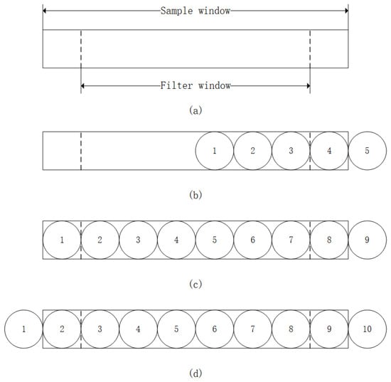
Figure 2.
Schematic diagram of sliding window filter process. (a) Sampling window. (b) Initial stage of sampling. (c) During Sampling. (d) Cyclic Sampling.
By employing a sliding window filter, noise and interference are effectively reduced, resulting in more stable and smoother data fluctuations. Additionally, each time a new data point was sampled, the earliest data point was removed, instantly updating the average and significantly speeding up the data processing workflow. Furthermore, the size of the sliding window can be flexibly adjusted based on real-time requirements and the desired data smoothness, achieving an optimal balance between processing speed and data quality.
2.2. Feature Correlation Verification
To enhance the accuracy and stability of deep learning models, it is crucial to clean redundant features after addressing missing values and outliers in the raw data. Pearson correlation coefficient and Spearman correlation coefficient are key indicators for measuring the correlation between two variables.
The Pearson correlation coefficient measures the linear relationship between two continuous variables. It assumes that the data are normally distributed and that the relationship between variables is linear [22]. Pearson’s r ranges from −1 to 1, where 1 indicates a perfect positive linear relationship, −1 indicates a perfect negative linear relationship, and 0 indicates no linear relationship.
The Spearman correlation coefficient, on the other hand, is a nonparametric measure of rank correlation. It assesses how well the relationship between two variables can be described using a monotonic function. Spearman’s also ranges from −1 to 1, where 1 indicates a perfect positive rank correlation, −1 indicates a perfect negative rank correlation, and 0 indicates no rank correlation.
In this study, the air-jet loom operations involve a significant amount of nonlinear data. The relationship between various features (such as machine type, speed, fabric width, etc.) and air consumption is likely to be nonlinear and complex. Therefore, the Spearman correlation coefficient is more appropriate as it does not assume a linear relationship and can better capture the monotonic relationships between features and air consumption. This choice ensures a more accurate and reliable feature selection process, enhancing the overall performance of the predictive model. This study utilizes the Spearman correlation coefficient, as shown in Formula (1).
Here, represents the Spearman correlation coefficient, is the difference in ranks for the -th pair of observations (i.e., the square of the rank difference for each pair of observations), and is the number of observations. Subsequently, specific feature fields were selected from the raw data of the air-jet loom for analysis, and the Spearman correlation coefficient matrix was plotted, as shown in Figure 3. By comparing the correlation coefficients of different features with air consumption, suitable features were selected.
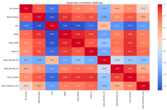
Figure 3.
Spearman correlation coefficient matrix for jet looms.
The analysis shows that factors highly correlated with air consumption include machine type, speed, fabric width, reed width, reed number, weft density, and total warp count.
2.3. Random Forest, XGBoost, and Linear Regression Models
Random forest integrates multiple decision trees and employs Bagging and feature randomness strategies to effectively reduce overfitting, enhancing model accuracy and stability. It performs better than single decision trees or other algorithms in handling high-dimensional data, nonlinear relationships, and imbalanced datasets. Additionally, it has strong noise resistance and features important evaluation capabilities. The algorithm can leverage multi-core processors for parallel computing, which leads to faster training speeds. However, random forest models can be complex and difficult to interpret, requiring substantial memory to store the trees. The algorithm’s structure is illustrated in Figure 4.
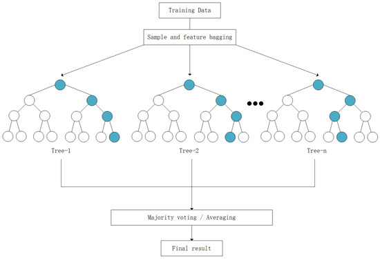
Figure 4.
Random forest algorithm structure.
As illustrated in Figure 5, the XGBoost network structure builds multiple decision trees iteratively. Each tree corrects the errors of the previous one, thereby gradually enhancing the model’s predictive capability. XGBoost uses gradient boosting to combine multiple weak learners, resulting in high performance and improved model accuracy. It includes regularization parameters to control overfitting and enhance generalization. XGBoost can efficiently handle missing values and is designed for speed and performance, making it suitable for large datasets. Despite its advantages, XGBoost can be complex to interpret and requires careful tuning of hyperparameters to achieve optimal performance.

Figure 5.
XGBoost network structure.
The objective of XGBoost is to minimize a given loss function , as shown in Equations (2) and (3). Here, represents the predicted value of sample , denotes the -th tree, and is the total number of trees.
To simplify calculations, XGBoost uses a second-order Taylor expansion to approximate the loss function, as shown in Equation (4). In this context, and represent the first and second derivatives of the loss function, respectively. The regularization term controls the model’s complexity, as depicted in Equation (5), where is the number of leaf nodes in the tree, is the weight of leaf node , and and are regularization parameters.
The optimal leaf node weight is calculated as shown in Equation (6).
The gain from splitting a node is calculated as shown in Equation (7), where and represent the sample sets of the left and right child nodes after the split, and represents the sample set of the current node.
Linear regression is a statistical analysis method used to model the relationship between two or more variables. It assumes a linear relationship between the independent variables and the dependent variable, meaning the dependent variable can be approximated by a linear combination of the independent variables. This relationship is illustrated in Figure 6 and calculated as shown in Equation (8). Here, is the intercept, representing the expected value of when all independent variables are zero. , ,…, are the regression coefficients, indicating the influence of each independent variable on the dependent variable. epsilonϵ is the error term, representing the difference between the actual and predicted values in the linear regression model. Linear algorithms are straightforward to implement and interpret, making them simple and efficient for large datasets. However, they have limited flexibility as they assume a linear relationship between features and the target variable, which may not hold for complex real-world data. They are also sensitive to outliers, which can significantly affect their performance.
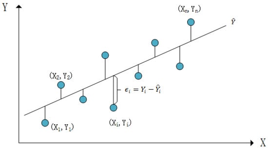
Figure 6.
Schematic diagram of linear regression variable relationship.
2.4. Model Selection
By comparing the R2 and Mean Squared Error (MSE) values of two models on the same training and testing sets, the model with better performance is selected for further training.
The R2, shown in Equation (9), is the coefficient of determination, a statistical measure of how well the regression model fits the data. Here, is the actual value of the iii-th observation, and is the model’s prediction for the -th observation. is the mean of all observations. If R2 is close to 1, it indicates that the model’s predictions are very close to the actual values, meaning the model has a high goodness of fit and good predictive performance. Conversely, if R2 is close to 0 or less than 0, it indicates poor predictive performance.
MSE is another common metric for evaluating the performance of regression models, as shown in Equation (10). Here, and are as previously defined. The larger the MSE value, the greater the model’s prediction error, and vice versa. The MSE shares the same unit as the target variable but in squared form, which amplifies the impact of larger errors, making predictions with larger deviations contribute more significantly to the overall error.
In summary, R2 and MSE are crucial metrics for evaluating model performance from different perspectives. R2 primarily reflects the explanatory power of the model, while MSE directly quantifies the discrepancy between the predicted and actual values. Although R2 is a valuable metric, it has certain limitations. R2 can be sensitive to outliers, which can distort the measure and give a misleading impression of the model’s performance. Additionally, R2 does not account for the complexity of the model and can be artificially increased by adding more variables, even if they do not contribute to better predictions. This can lead to overfitting, where the model fits the training data well but performs poorly on unseen data.
In this study, the preprocessing steps, including the use of the sliding window filter, mitigate the impact of outliers and data anomalies. This ensures that R2 retains its explanatory power even in the presence of sporadic abnormal points. To prevent overfitting and ensure that the model can adapt well to new weaving process parameters, incremental learning is necessary. Incremental learning allows the model to continuously update and refine itself as new data become available, enhancing its ability to generalize and perform well on unseen data. Moreover, MSE is used alongside R2 to provide a more comprehensive evaluation of model performance, as it directly quantifies the prediction error.
R2 is widely used in engineering and various regression modeling tasks to assess model performance, demonstrating its utility in predictive analytics and modeling efforts.
2.5. Incremental Learning Strategy
The limitations of a single model in complex system predictions often stem from extreme sensitivity to initial conditions and random fluctuations during training. To overcome this challenge, we adopted the successful ensemble learning approach from the neural network domain and designed an incremental learning update strategy. This strategy enables the model to continuously learn and self-improve as the amount of training data increases. The overall learning strategy for this study is illustrated in Figure 7.
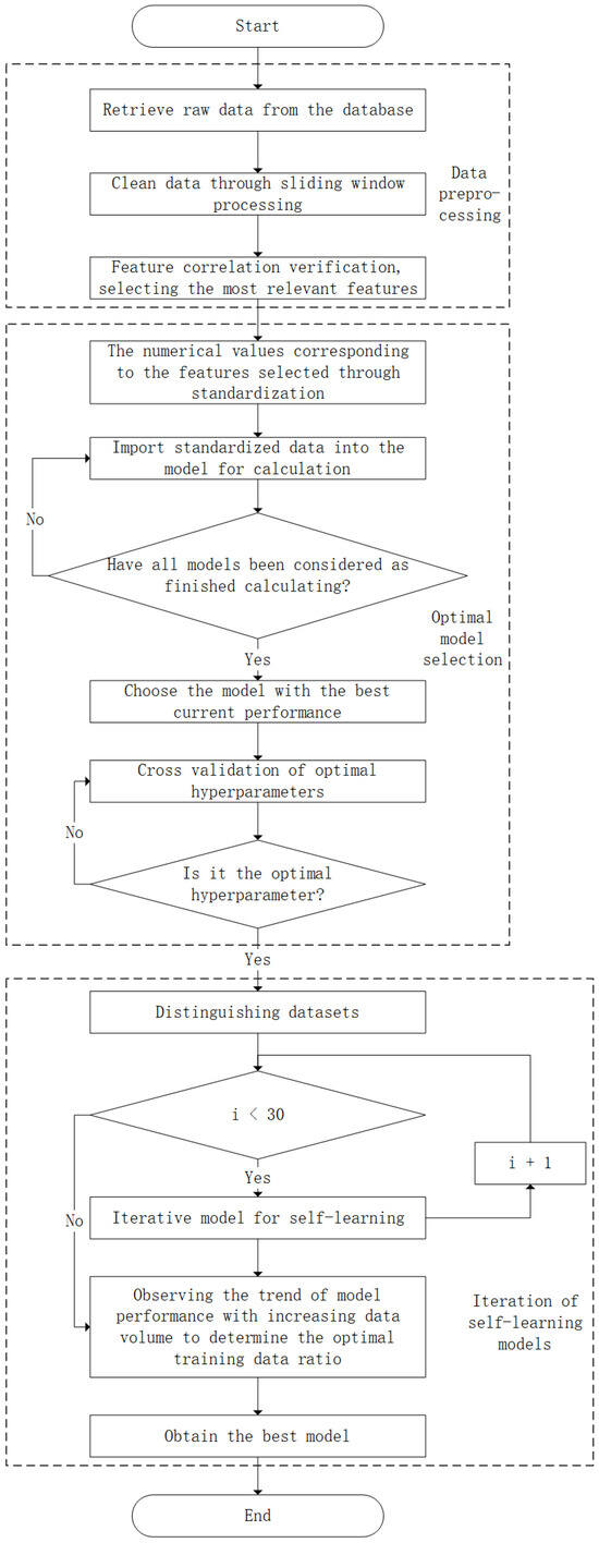
Figure 7.
Flowchart of research on the overall learning strategy.
Here are the explanations of the model update steps and the conditions for triggering incremental learning:
Model Update Steps:
- Initial Model Training:
Data Preparation: Collect and preprocess the initial dataset, ensuring it is cleaned and normalized, addressing missing values and outliers.
Model Training: Train the initial random forest model using the preprocessed data to establish a baseline model.
- 2.
- Incremental Data Collection:
Continuous Monitoring: Continuously collect new data from the air-jet looms during their operation. These data reflect the latest operating conditions and any changes in the production environment.
Preprocessing: Ensure the new data are preprocessed to match the format and quality of the initial dataset.
- 3.
- Model Update Mechanism:
Data Integration: Integrate the newly collected data with the existing dataset, appending the new data and preprocessing them accordingly.
Batch Update: Retrain the model using the combined dataset, incorporating both the existing and new data. This can be performed periodically or triggered by specific conditions.
- 4.
- Validation and Evaluation:
Validation: After each update, validate the model using a separate validation set to ensure the updates improve the model’s performance.
Performance Metrics: Evaluate metrics such as R2 and MSE to monitor the model’s performance and ensure it remains accurate and reliable.
- 5.
- Dynamic Adaptation:
Feedback Loop: Implement a feedback loop where the model’s predictions and actual outcomes are continuously compared, and discrepancies are used to further refine the model.
Adaptation to Changes: Ensure the model dynamically adapts to new patterns and changes in the data, maintaining its accuracy and reliability over time.
Incremental Learning Conditions:
- 1.
- Data Volume Threshold:
Condition: An update is triggered when new data amounting to at least 10% of the initial training dataset are collected.
Reason: Ensures sufficient new information is available to make meaningful updates without overwhelming the model with too frequent changes.
- 2.
- Performance Degradation:
Condition: A noticeable drop in performance metrics (e.g., R2 or MSE) during validation tests.
Reason: Indicates that the model is becoming less accurate, possibly due to changes in the underlying data distribution or new patterns emerging.
- 3.
- Periodic Updates:
Condition: Regular time intervals, such as weekly or monthly updates.
Reason: Ensures the model stays current with the most recent data, even if specific performance degradation is not observed.
- 4.
- Operational Changes:
Condition: Significant changes in production processes, such as new yarn types, changes in loom settings, or other operational adjustments.
Reason: These changes can significantly affect air consumption patterns, necessitating a model update to maintain accuracy.
3. Data Preparation
3.1. Preparation of Raw Data
The data for this study were sourced from the production records of a textile factory, collected at five-minute intervals. Data were gathered from 188 machines in the workshop and 26 different types of fabrics. The data collection was grouped based on shifts, with one shift starting at 06:45 and the other at 17:45 each day, continuously collected over a period of 30 days.
First, the raw data need to be cleaned using a sliding window filter. Figure 8 shows the cleaned data results for two of the machines. The sliding window filter effectively handles both sudden and sustained oscillations, demonstrating its robustness.
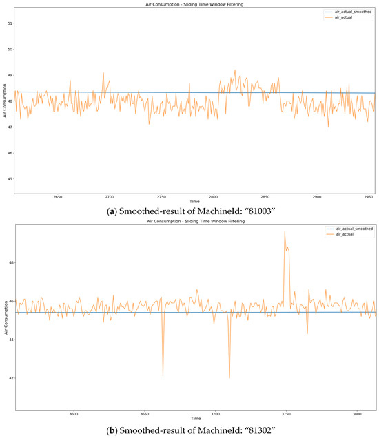
Figure 8.
Diagram of smoothed result.
After data cleaning, the distribution of all gas consumption values is shown in Figure 9a. Additionally, standardizing the data is essential when training the model, as these algorithms are sensitive to the scale of the input data. Therefore, this study uses StandardScaler for data normalization, as shown in Figure 9b. The data transformation process is described in Equation (11), where is the original feature value, is the mean of the feature, is the standard deviation, and is the normalized feature value. This standardization centers the data around zero mean and unit variance.
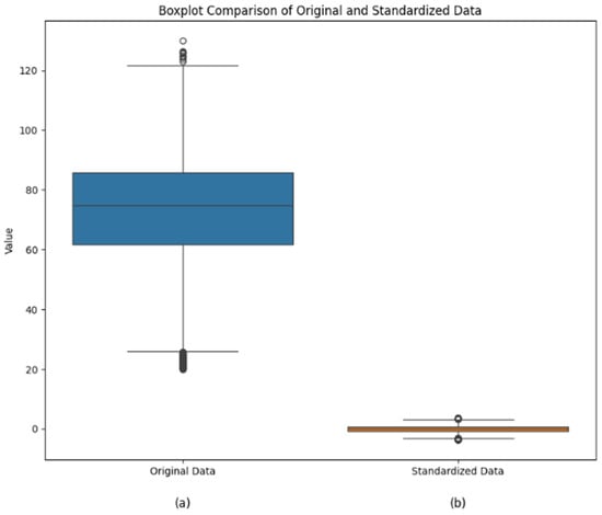
Figure 9.
Standardization comparison of gas consumption data.
The graphs clearly show that after standardization using StandardScaler v1.5.0, the range of air consumption values is significantly reduced. Standardization eliminates the scale differences between different features, allowing all features to be compared on the same scale. This prevents features with larger value ranges from unduly influencing the model.
3.2. Model Comparison
To select the appropriate model, this study used the standardized data processed in Section 3.1 to train three models: random forest, XGBoost, and linear regression. The performance of these models was evaluated based on whether a sliding window filter was used for data cleaning, as well as a comparison between traditional model features and data-driven full features. The results, shown in Table 1, validate the feasibility of the methods used in this study.

Table 1.
Prediction results under different features and methods.
The random forest model achieves the highest R2 value (0.950) and the lowest MSE (16.239) when all features are used with the sliding window filter, indicating it has the best predictive performance among the three models. XGBoost also performs well with a slightly lower R2 (0.948) and higher MSE (16.956), while linear regression shows the lowest performance with an R2 of 0.928 and a higher MSE of 23.541, demonstrating its limitations in capturing complex relationships in the data.
When certain features are removed, both XGBoost and random forest models show a significant decrease in performance, with lower R2 values (0.904 and 0.905, respectively) and higher MSE values (32.994 and 32.369, respectively). This highlights the importance of including all relevant features to improve model accuracy and reliability.
Without the sliding window filter, the performance of both XGBoost and random forest models deteriorates compared to when the filter is used, as indicated by lower R2 values (0.904 and 0.906) and higher MSE values (32.861 and 32.244). This demonstrates that the sliding window filter effectively improves data quality, leading to better model performance.
The results in Table 1 highlight the importance of including all relevant features and the effectiveness of the sliding window filter in enhancing model performance. Additionally, ensemble models like random forest and XGBoost outperform linear regression, indicating their superior capability to capture complex and nonlinear relationships in the data.
The table shows that the random forest model performs the best when trained with all features and after data cleaning using the sliding window filter.
3.3. Hyperparameter Optimization
Hyperparameter optimization involves systematically exploring and fine-tuning the configuration parameters of a model to significantly enhance its performance, accelerate the training process, improve generalization to new data, and increase robustness against external disturbances. This ensures that the model achieves optimal or near-optimal performance on both specific tasks and diverse datasets while minimizing manual trial and error, thereby automating and streamlining model training. In this study, GridSearchCV was employed to perform cross-validation over a predefined grid of hyperparameters, systematically evaluating the model’s performance under different parameter combinations. The optimized hyperparameters for the random forest model are shown in Table 2. The hyperparameters listed in Table 2 were selected to optimize model performance while balancing complexity and generalization. Bootstrap was enabled to increase model diversity and reduce overfitting. A max_depth of 10 was chosen to capture sufficient detail without excessive complexity. Min_samples_leaf was set to 4 to prevent overfitting by ensuring each leaf had enough samples. Min_samples_split was set to 2 to allow useful splits without making the model too complex. Finally, n_estimators was set to 100 to ensure stable and accurate predictions. These values were determined through cross-validation, optimizing the model’s performance on the validation set.

Table 2.
The optimal hyperparameters of a random forest model.
3.4. Dynamic Model Updating
3.4.1. Overview of Dynamic Learning
In the code, the amount of training data is gradually increased through iterations, starting from 70% and adding 1% with each iteration until reaching 100%, as shown in Figure 10a. In an incremental learning scenario, the model continuously learns and improves as more data arrives. To validate this approach, it is compared with a non-iterative method, as shown in Figure 10b. The code calculates the predictive performance, R2 and MSE, for both iterative and non-iterative models, as presented in Table 3. By continuously monitoring these metrics, it is possible to detect when the model starts overfitting or its performance declines, triggering parameter adjustments. This approach ensures that the model adapts promptly to changes in the dataset rather than remaining fixed in a specific training phase.
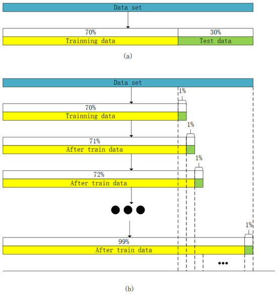
Figure 10.
Diagram of incremental learning process. (a) Data Partitioning. (b) Incremental Learning Process.

Table 3.
Static and dynamic models predict R2 and difference.
3.4.2. Dynamic Learning Experiment Results
Based on the method described in the previous section, we conducted experiments using real data that were cleaned using a sliding window filter. The cleaned data were split into a 7:3 ratio, with 70% used to train a full-feature random forest model and the remaining 30% as the test set, divided into 30 parts. During this period, two minor adjustments, involving changes in the types of fabrics processed, were made in the workshop. The static method used the initial model to predict each test set, while the dynamic method retrained the model after each prediction by adding the current test set to the training data. Table 3 presents the R2 values for each test set using both static and dynamic methods, along with their differences (dynamic minus static). To visualize the changes, an R2 difference line chart is shown in Figure 11. Observing the line chart, the dynamic model performs similarly to the static model when workshop data fluctuations are relatively small. However, when significant changes occur, such as multiple machines undergoing adjustments, the dynamic model significantly outperforms the static model, demonstrating the reliability of the incremental learning approach in adapting to dataset variations.
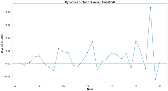
Figure 11.
Chart of static and dynamic model prediction R2 difference fluctuation.
4. Results
The flowchart of the innovative method is shown in Figure 7, with experimental results presented in Figure 3, Figure 8, Figure 9 and Figure 10. This study developed a novel air consumption prediction method for air-jet looms. By leveraging a data-driven approach, we identified a broader range of features compared to traditional model-based methods, resulting in a prediction model that closely aligns with physical realities. On the test set, the R2 improved from 0.905 to 0.950, and the MSE decreased from 32.369 to 16.239. A well-configured sliding window smoothed the air consumption for each machine, reducing data collection errors caused by frequent starts and stops. With the application of the sliding window filter, the random forest model built on all features showed significant improvements, with the R2 increasing from 0.906 to 0.950 and the MSE decreasing from 32.244 to 16.239. The decision tree method further enhanced the prediction model by capturing complex nonlinear relationships in the air consumption process, thereby improving predictive capabilities.
Given the variety-focused nature of the weaving workshop, where production varieties are complex and variable, feature analysis revealed a significant correlation between air-jet loom air consumption and product variety. Therefore, this study utilized incremental learning to enhance the prediction model, making it more robust for short-term predictions. Although the study achieved significant success in the short-term prediction of overall workshop air consumption, it is based on the data-driven exploration of overall workshop consumption. This serves as a foundation for analyzing and predicting workshop air consumption and adjusting air compressor strategies, achieving transparency in workshop air consumption costs. Despite the large volume of actual workshop data, the multi-dimensional features remain discrete, failing to fully capture the complex nonlinear relationships of air-jet loom air consumption. Furthermore, air consumption is influenced by other factors such as temperature and humidity, air compressor frequency conversion strategies, and operator habits.
Therefore, the current prediction model may exhibit short-term dataset overfitting. Future advancements in smart manufacturing are expected to enable the perception of more data dimensions. With the support of big data, the complex nonlinear relationships of air consumption can be explored, providing model support for cost optimization in product design and manufacturing processes, further promoting green production and low-carbon development.
Author Contributions
Conceptualization, B.Y. and X.H.; methodology, C.S.; software, L.F.; validation, B.Y., Z.W., and L.F.; formal analysis, C.S.; investigation, C.S.; resources, C.S.; data curation, L.F.; writing—original draft preparation, X.H.; writing—review and editing, B.Y.; visualization, Z.W.; supervision, B.Y.; project administration, C.S. All authors have read and agreed to the published version of the manuscript.
Funding
This research received no external funding.
Data Availability Statement
The original contributions presented in the study are included in the article. Further inquiries can be directed to the corresponding author.
Conflicts of Interest
Author Chunya Shen was employed by the company Zhejiang Kangli Automation Technology Co., Ltd. The remaining authors declare that the research was conducted in the absence of any commercial or financial relationships that could be construed as a potential conflict of interest.
Abbreviations
The following abbreviations are used in this manuscript:
| ANFIS | Adaptive neuro-fuzzy inference systems |
| CNC | Computer numerical control |
| CPU | Central processing unit |
| CV | Computer Vision |
| EEMD | Ensemble Empirical Mode Decomposition |
| GEP | Gene Expression Programming |
| I/O | Input/output |
| LSTM | Long short-term memory |
| MSE | Mean Squared Error |
| NARX | Nonlinear Autoregressive with Exogenous Input |
| PCA | Principal component analysis |
| sCARS | Stability Competitive Adaptive Reweighting Sampling |
| SCN | System Change Number |
| STW | Sliding Time Windows |
References
- Wang, L.; Li, C.; Tang, B. Research on the Development Characteristics and Dynamic Mechanisms of the World Textile Industry. Melliand 2005, 5, 4. [Google Scholar]
- Jabbar, A.; Ahmed, S.; Hussain, T.; Haleem, N.; Ahmed, F. Statistical Model for Predicting Compressed Air Consumption on Air-Jet Looms. J. Eng. Fibers Fabr. 2014, 9, 155892501400900306. [Google Scholar] [CrossRef]
- Göktepe, Ö.; Bozkan, O. Study on Reduction of Air Consumption on Air-jet Weaving Machines. Text. Res. J. 2008, 78, 816–824. [Google Scholar] [CrossRef]
- Gunarathna, D.; Kumari, R.; Subawickrama, S.; Fernando, E.; Jayawardana, T. Modeling of compressed air requirement for different weft yarns on air jet weaving. In Proceedings of the 2017 Moratuwa Engineering Research Conference (MERCon), Moratuwa, Sri Lanka, 29–31 May 2017; pp. 193–198. [Google Scholar]
- Xu, H.Y. Discussion on Energy Consumption of Jet Loom and Reduction of Auxiliary Nozzle Air Consumption. J. Text. Res. 2010, 31, 126–130. [Google Scholar] [CrossRef]
- Lu, Y.; Sheng, B.; Fu, G.; Luo, R.; Chen, G.; Huang, Y. Prophet-EEMD-LSTM based method for predicting energy consumption in the paint workshop. Appl. Soft Comput. 2023, 143, 110–447. [Google Scholar] [CrossRef]
- Kim, J.Y.; Cho, S.B. Electric Energy Demand Forecasting with Explainable Time-series Modeling. In Proceedings of the 2020 International Conference on Data Mining Workshops (ICDMW), Sorrento, Italy, 17–20 November 2020. [Google Scholar]
- Pan, J.; Li, C.; Tang, Y.; Li, W.; Li, X. Energy Consumption Prediction of a CNC Machining Process With Incomplete Data. IEEE/CAA J. Autom. Sin. 2021, 8, 987–1000. [Google Scholar] [CrossRef]
- Babanova, I.S.; Tokarev, I.S.; Abramovich, B.N.; Babyr, K.V.J.I. Electric Energy Consumption Modes Forecasting and Management for Gas Industry Enterprises Based on Artificial Intelligence Methods. In Proceedings of the 2021 IEEE Conference of Russian Young Researchers in Electrical and Electronic Engineering (ElConRus), St. Petersburg, Moscow, Russia, 26–29 January 2021. [Google Scholar]
- Hussain, T.; Jabbar, A.; Ahmed, S. Comparison of regression and adaptive neuro-fuzzy models for predicting the compressed air consumption in air-jet weaving. Fibers Polym. 2014, 15, 390–395. [Google Scholar] [CrossRef]
- Yuan, M.; Yu, G.; Guo, Q.; Liu, J.; Yuan, M.; Li, J. Research on Energy Consumption Prediction of Forming Machine Based on sCARS NARX. Control. Eng. China 2024, 1–7. [Google Scholar] [CrossRef]
- Shao, C.; Ning, J. Construction and Application of Carbon Emission Prediction Model for China’s Textile and Clothing Industry Based on Improved WOA-LSTM. J. Beijing Inst. Fash. Technol. (Nat. Sci. Ed.) 2023, 43, 73–81. [Google Scholar] [CrossRef]
- Li, X. Design and Development of Predictive Maintenance System for Spinning Machine Based on Energy Consumption Parameters. Master’s Thesis, Zhengzhou University of Light Industry, Zhengzhou, China, 2023. [Google Scholar]
- Svetnik, V.; Liaw, A.; Tong, C.; Culberson, J.C.; Sheridan, R.P.; Feuston, B.P. Random Forest: A Classification and Regression Tool for Compound Classification and QSAR Modeling. J. Chem. Inf. Comput. Sci. 2003, 43, 1947–1958. [Google Scholar] [CrossRef] [PubMed]
- Fernandez-Delgado, M.; Cernadas, E.; Barro, S.; Amorim, D. Do we Need Hundreds of Classifiers to Solve Real World Classification Problems? J. Mach. Learn. Res. 2014, 15, 3133–3181. [Google Scholar]
- Ahmed, N.; Huan, S.; Kah, L.; Sung, K. Incremental Learning with Support Vector Machines. In Proceedings of the Workshop on Support Vector Machines at the International Joint Conference on Artificial Intelligence (IJCAI-99), Stockholm, Sweden, 2 August 1999. [Google Scholar]
- Tang, L.; Cai, F.; Ouyang, Y. Applying a nonparametric random forest algorithm to assess the credit risk of the energy industry in China. Technol. Forecast. Soc. Chang. 2019, 144, 563–572. [Google Scholar] [CrossRef]
- Hakala, K.; Kaewphan, S.; Bjorne, J.; Mehryary, F.; Moen, H.; Tolvanen, M.; Salakoski, T.; Ginter, F. Neural Network and Random Forest Models in Protein Function Prediction. IEEE/ACM Trans. Comput. Biol. Bioinform. 2022, 19, 1772–1781. [Google Scholar] [CrossRef] [PubMed]
- Phan, Q.-T.; Wu, Y.-K. Short-term Solar Power Forecasting Using XGBoost with Numerical Weather Prediction. In Proceedings of the 2021 IEEE International Future Energy Electronics Conference (IFEEC), Taipei, Taiwan, 16–19 November 2021; pp. 1–6. [Google Scholar]
- Hussain, N.; Qasim, A.; Akhtar, Z.-u.-d.; Qasim, A.; Mehak, G.; del Socorro Espindola Ulibarri, L.; Kolesnikova, O.; Gelbukh, A. Stock Market Performance Analytics Using XGBoost. In Proceedings of the Advances in Computational Intelligence; Springer: Cham, Switzerland, 2024; pp. 3–16. [Google Scholar]
- Lee, C.; Lin, C.; Chen, M. Sliding window filtering: An efficient method for incremental mining on a time-variant database. Inf. Syst. 2005, 30, 227–244. [Google Scholar] [CrossRef]
- Xu, W.C. A Review on Correlation Coefficients. J. Guangdong Univ. Technol. 2012, 29, 12–17. [Google Scholar] [CrossRef]
Disclaimer/Publisher’s Note: The statements, opinions and data contained in all publications are solely those of the individual author(s) and contributor(s) and not of MDPI and/or the editor(s). MDPI and/or the editor(s) disclaim responsibility for any injury to people or property resulting from any ideas, methods, instructions or products referred to in the content. |
© 2024 by the authors. Licensee MDPI, Basel, Switzerland. This article is an open access article distributed under the terms and conditions of the Creative Commons Attribution (CC BY) license (https://creativecommons.org/licenses/by/4.0/).