Competition Between Geographically Spread Charge Point Operators for Battery Electric Trucks—Estimations of Prices and Queues with an Agent-Based Model

Abstract

In light of the drawbacks of using fossil fuel, this paper investigates the competition between geographically spread charge point operators for future battery electric long-haul trucks along one of the busiest highways in Sweden. This is achieved using an agent-based model where trucks try to charge for a low price and still avoid queues in order to complete their transport mission. The charging need for a typical day at full electrification is derived from data from the Swedish Transport Administration. This typical day is simulated several times and in between these iterations the charge point operators adjust their prices and number of chargers, aiming to increase their profit. After a sufficiently long time of competition, a quasi-equilibrium is reached where, for example, prices and queueing times can be studied. The goal of the study is to estimate conditions for trucks and charge point operators in a future public fast-charging market. Assuming a price for electricity of 0.08 EUR/kWh, the results indicate that a system with low queuing problems is attainable with a mean price of 0.27 EUR/kWh or lower for public fast charging. It is also found that the behaviour of haulage companies, as a collective, can affect the future fast charging market to a great extent. If the hauliers are price-sensitive, they will be offered a low mean price, down to 0.11 EUR/kWh, but with queues, while if they are queue-sensitive, there will be almost no queues, but they will pay more to charge.

1. Introduction

Combustion of fossil fuels has likely affected the Earth’s climate system [1]. Health impacts due to deteriorated air quality have been expressed in the literature [2] and, in addition, humanity will probably run out of oil in less than 30 years [3]. A part of the solution to these grave problems could be to replace today’s commercial diesel trucks with battery electric ones. This approach is reasonable since many studies have shown that these trucks could become a cost-competitive alternative [4,5,6,7,8] able to operate without fossil fuel. The driving pattern of the trucks strongly impacts the effectiveness of battery electric trucks [4] and trucks that have close to uniform driving patterns are especially suitable for electrification [4,9]. Hydrogen trucks could be a solution [10] but, in most cases, battery electric trucks seem to be the better option [11] and they seem to have good feasibility in [12]. However, for extra-long trips with heavy-duty trucks, fuel cells may be the better option [13]. All in all, battery electric trucks seem promising but will likely not give the lowest total cost of ownership in all situations and thus different powertrains could be taken into consideration depending on the transport missions of trucks.

Previous studies emphasise other important factors for the battery electric vehicles to be cost-effective. These are the possible number of cycles the battery can perform [14], the price of the battery [15], and its size [4,16]. Moreover, the public fast-charging price could have a strong impact on the battery sizing, charging strategy, and cost-effectiveness [5]. Sufficiently high utilisation of the chargers is needed for reasonable prices on public fast charging [5] and a prerequisite for the installation to be worthwhile [17]. Some advantages of increased charging price during rush hours were presented in a previous study [18], including better meeting the demand, thus avoiding queues, and increasing profit, provided some customers change their charging due to the price variations. Fast charging is expected to be necessary for long-haul trucks [19] and will be available with the new MCS-standard, which will allow charging power up to 3.75 MW. This power is much greater than the currently available charging power and the full MCS-standard is even suggested to be oversized for truck applications [20]. A recently performed study [21] shows a promising result, namely, for public fast chargers, it seems possible to achieve high charger availability and simultaneously high charger utilisation. Another result from [21] is that the trucks’ willingness to avoid queues is important for the charger availability; this result can also be seen in another study [22]. In [21], a system of public fast chargers and charging trucks was investigated. The number of chargers was tuned manually and thus the question of whether utilisation would be that high in a free competitive market was raised. Recently, this question was addressed, and it was found that it seems likely that the free market will build enough chargers to meet demand during rush hours, still with high utilisation of the chargers [23]. Reference [23] suggested, based on an agent-based model supported by analytical calculations, that a spot market would lead to large variations in charging price over the day. However, the investigations only include competition between two charge point operators (CPOs) at the same site; it is unclear if the large variations in price will still be present if one includes more competing CPOs spread out geographically. In the present paper, the work carried out in [23] is further developed so that more than two competing CPOs are included as well as geographically spread CPOs to fill the aforementioned research gap. In addition, the CPOs in this paper can change their prices in leaps, greater than the allowed price change in Ref. [23]. The price for public fast charging is one of the most important factors for battery electric trucks to be cost-effective according to the authors of the current paper. Moreover, it will likely impact their charging strategy. Further, large variations in charging price during the day might impact hauliers’ route planning. Today’s market is in an early state and future price levels and variation over the day could differ substantially from how they are currently. Knowledge of this is vital before hauliers can plan for large-scale electrification. Therefore, it is important to either confirm or to question the large price variations found in [23] as well as the price level.

In the present paper, an agent-based model is used to investigate the interactions between CPOs and charging trucks. Agent-based models have been used for a wide range of problems, for example, to study segregation in society [24], competition in biology [25], and disease spread [26]. The use of an agent-based model is justified by the argument that it is easier and more straightforward to find reasonable rules for agents than to create a reliable macroscopic model. Maybe there are other methods that could be successful as well. However, when considering classical methods from game theory, we think that such an approach will become unmanageable with our number of agents and actions. An agent-based model is a better option to handle this huge number of combinations. Also, formulating charging problems as a pure optimisation problem and then aiming for the optimum has been achieved in the literature [27]. In this case, the minimum number of chargers was found for charging electric buses in cities. However, difficulties with treating the interactions between charging trucks and CPOs as a pure optimisation problem are discussed in chapter 5.3 in Ref. [23]. The problem with this approach is that the optimum setup of prices and number of chargers differ depending on the competitors set up. The fact that there are several actors, each one striving to fulfil its goal and where many possible actions affect the other actors makes an agent-based model a natural choice since it is a method that aims to mimic reality. From an agent-based model one can, only by designing rules on the microscopic level, obtain macroscopic results and draw system-level conclusions, which makes agent-based models a powerful tool in this context.

The key contribution to the research field is that several competing CPOs, spread geographically, are investigated. Some important results from this paper are that the price variation over the day for public fast charging will likely be less extreme in reality than what was found in Ref. [23] and it seems likely that the average fast charging price for long-haul trucks will be around 0.27 EUR/kWh or lower along roads with similar charging demand as the one studied. This paper is structured as follows: In Section 2, a brief introduction to the model is given and the analyzed traffic flow is introduced. Section 3 describes the used agent-based model, in which the trucks can either be price- or queue-sensitive. The results are presented in Section 4 and discussed and summarised in Section 5. In Section 6, further analyses of the case with queue-sensitive trucks are presented by considering non-modelled flow variations over the year and evaluating the profitability of the CPOs. Limitations of the study and further developments are discussed in Section 7 and finally the conclusions are presented in Section 8.

2. Introduction to the Agent-Based Model and Charging Demand

The method and conclusions in this study are quite general, but only one flow of charging trucks is analysed. This truck flow, and the resulting charging demand, are meant to represent the charging need for all long-haul trucks driving on the Swedish highway E4 on a typical weekday in the case of full electrification of the truck fleet. This road connects the two cities Helsingborg and Stockholm and is one of the busiest highways in Sweden; see Figure 1. The charging demand is derived from data from the Swedish Transport Administration [28]. There are competing CPOs along the highway. The CPOs, as well as the trucks, are agents. The CPOs change their number of chargers and prices according to a set of rules with the aim of improving profit. The trucks select CPOs in order to complete their transport task while simultaneously trying to minimise their time for queuing and costs for charging. To briefly summarise the main idea of the simulation: the CPOs start with a number of chargers at their station and a setup of charging prices that may vary each hour. Then, the typical day is simulated so that the trucks select CPOs to complete their transport task while minimising the cost for charging and time for queuing. Between each simulation of the typical day, half of the CPOs can update their prices and number of chargers according to a set of rules after which the day is simulated once again. If a CPO that made changes increased its profit, it will keep the new price and number of chargers; if not, it will go back to the old setup. This procedure will be repeated until the system reaches something similar to a market equilibrium where one may study, for example, prices and queues in the system.

The traffic flow, i.e., the charging demand used in the simulations, is very similar to the flow used in Ref. [21] and found by the same method (involving some randomness). The traffic flow is meant to represent the traffic of long-haul trucks on a typical weekday along road E4 in the case of full electrification. The flow consists of 4355 trucks, each with a usable battery capacity of 500 kWh. Each truck has a transport task between two of the following cities: Helsingborg, Jönköping, Linköping, and Stockholm—see Figure 1. In the simulations, the road is considered a one-dimensional line with the origin placed at Helsingborg. The fact that the full road network is not considered can on the one hand seem like a weakness for the completeness of the model, but this simplification was necessary to limit the scope of the paper and to make it more comparable to Ref. [21]. Also, the method for finding the traffic flow developed in Ref. [21] takes the larger connecting roads into consideration when finding the traffic flow. Each truck has an individual start state of charge (SoC) and a required SoC at its destination. Most of the trucks will charge once during their trip, some will charge twice, and some trucks will not charge at all. A more detailed explanation of the simulated flow, and the method to generate it, is found in [21].

3. Description of the Agent-Based Model

This section describes the agent-based model that simulates the trucks and CPOs. Roughly, one may say that this model is a combination of the agent-based models used in Refs. [21,23] but with some important differences. Due to these differences, the model is described largely from scratch in this paper as well.

3.1. Assumptions

The model tries to predict prices and queues at public fast-charging stations along the highway E4 after a long time of competition. However, only one road is investigated and not the full road network. This is necessary to keep the scope of the problem reasonable and to expend a sensible amount of work investigating it. Generally, limiting a problem also makes it easier to explore basic behaviour. The road has a length of $S=553$ km. All the trucks in the simulation have a speed of $v=75$ km/h, a usable battery capacity of $B_{cu}=500$ kWh, and an energy consumption of ${\displaystyle \frac{\Delta E}{\Delta x}}=1.5$ kWh/km. The last three of the mentioned parameters are, in reality, not the same for all trucks. However, the authors believe that these values are reasonable for future heavy-battery electric trucks. On a system level, many of the random individual variations will cancel out since a large fleet of trucks is analysed. However, the systematic variations in energy consumption will not cancel, such as during days with cold weather, and such effects are not directly modelled. In the nomenclature list at the end of this paper, the parameter values used for the simulations are shown. The model is run through the typical day twice each time the day is simulated in order to create good initial conditions. The first run of the day starts with empty charging stations and roads. The aim is to start the second run of the typical day with trucks on the road and in the charging stations. The results presented in this paper are from the second runs of the day.

In reality, there are regulations for how long drivers are allowed to drive before they must take a break and the shortest allowed break before the driver may continue driving. For example, Regulation (EC) No 561/2006 [29] stipulates that drivers must take a break after no more than four and a half hours of driving, which is not explicitly modelled, but even with a full battery of the selected size, a truck cannot operate for more than four and a half hours without charging.

There are charging sites along the road, at each site there are two competing CPOs, and the distance between each site is $\Delta s$. The two CPOs at sites closest to the origin (Helsingborg) are called CPO 1 and CPO 2, the CPOs at sites at a distance $\Delta s$ away are called CPO 3 and CPO 4, and so on; see Figure 2 for an example with three charging sites. In this paper, all the chargers deliver a power of $P=700$ kW during a charging session to all trucks regardless of SoC. Typically, this requires 900 kW chargers and implies that a truck will charge its whole usable capacity in 43 min. Notice that, in this paper, each CPO is in competition with all the others. In reality, it is likely that there is cooperation between some CPOs with the same owner.

3.2. The Charging Behaviour of the Trucks

Each truck agent will in all simulations act according to the rules presented below:

1.

The truck agents will only charge when it is needed to complete their mission and only charge the necessary amount of energy to have the required SoC at their destination.

2.

The truck agents will not charge more times than necessary. This rule implies that none of the trucks will charge more than twice (as mentioned in earlier in the text).

3.

A truck agent that needs to charge twice will always take a full charge the first time.

Later, more rules for how the trucks select a CPO will be presented. Those rules will differ between simulated scenarios.

3.3. Simulation of the Typical Day

When simulating the typical day, a time-iterating, agent-based model is used. At the start of the simulation, the time t equals $-24$ h. The typical day is simulated twice to obtain proper initial conditions when it is simulated the second time. The time then increases in increments of $\Delta t$ until it reaches the time $t=T=$ 24 h. In the simulations conducted in this paper, the time step is one minute. The fact that the time step is not smaller can result in some small errors, like that the battery might be overcharged by up to 2%. Since the authors do not think that this affects the result to a great extent, the size of the time step is considered sufficiently small.

At the time $-24$ h (start of the first run of the typical day), the charging stations and roads are empty. Before each time step, truck agents enter the road according to the traffic flow. Each truck agent that has the maximum distance $v·\Delta t$ to a charging site, and selects that site for charging, can charge or stand in queue to charge there.

The trucks that are driving update their location and SoC according to

$$X_i(t+\Delta t)=X_i\left(t\right)+v·\Delta t$$

(1)

where $X_i$ is the location of truck i and

$$So{C}_i(t+\Delta t)=So{C}_i\left(t\right)-v·\Delta t·{\displaystyle \frac{dE}{dx}}/B_{cu}$$

(2)

where $So{C}_i$ is the SoC of truck i. Then, there are queuing truck agents waiting to charge that update their queuing time. These are neither charging nor moving, but the truck agents’ total queuing time is increased by adding the queuing time $\Delta t$. Also, there are truck agents that are charging and they update their SoC according to

$$So{C}_i(t+\Delta t)=So{C}_i\left(t\right)+P·\Delta t/B_{cu}.$$

(3)

For each CPO j, the total energy delivered from that CPO, $E_{charger}^j$, is updated according to

$$E_{charger}^j(t+\Delta t)=E_{charger}^j\left(t\right)+M_j\left(t\right)·P·\Delta t$$

(4)

where $M_j\left(t\right)$ is the number of charging trucks at station j at time t. Also, the net income for each CPO j, $I_{income}^j$, is updated according to

$$I_{income}^j(t+\Delta t)=I_{income}^j\left(t\right)+\sum _i(pric{e}_i^j-C_e)·P\Delta t,$$

(5)

where $pric{e}_i^j$ is the price for truck i that charges at CPO j and $C_e$ is the price for electricity paid by the CPO. In this paper, $C_e$ is set to 0.08 EUR/kWh. Notice that the two equations above are only used for the second simulation of the day when $t\ge 0$. Before commencing a new time step, the truck agents that are finished charging leave the charging station and the queue is updated. If a truck that has reached its target SoC only needs to charge one time, it is now removed from the simulation. If it must charge two times, it will continue along the road until it charges its second time and will then subsequently be removed after the charging session. When the whole day is simulated, the profit for each CPO j, $I_{\mathit{profit}}^j$, is calculated as follows:

$$I_{\mathit{profit}}^j=I_{income}^j\left(T\right)-{\displaystyle \frac{9}{7}}·P·C_{ch}·N_{tot}^j,$$

(6)

where $C_{ch}=0.32$ €/kW is the total cost per day per kilowatt of installed power for the chargers and grid connection. The factor ${\displaystyle \frac{9}{7}}$ compensates for the fact that a 900 kW charger is required to deliver 700 kW on average and $N_{tot}^j$ is the total number of chargers at CPO j.

Notice that the investigated day will be simulated many times during one simulation—i.e., the simulation of the typical day will be iterated many times. The CPOs will have the opportunity to adjust their prices and the number of chargers between the iterations. The goal is to study prices and queues among other variables after a sufficiently long time of competition such that the market may converge to an equilibrium. Still, there is no guarantee that the market ends up in a true steady state. It may also converge to a quasi-equilibrium, with repeated, small variations around an equilibrium state.

3.4. Repeated Simulations of the Typical Day

Along the road, there are charging sites, with equal distance $\Delta s$ between them. At each site, there are two CPOs with an individual number of chargers and individual prices. The prices can vary each hour where the first hour corresponds to the time between midnight and 1 a.m. and the second hour to the time 1 a.m. to 2 a.m. and so on. The typical day is simulated or iterated many times. In between the iterations, one of the CPOs at each site can change its number of chargers and change its prices. For the next iteration, the other CPO at each site can make changes. The rules for how the CPOs make these changes are presented in a coming subsection, while the overall simulation is described in the following paragraph.

Below, the procedure of the simulation is described on a high level and it includes the following steps:

1.

Initial conditions for the CPOs are set. These are individual prices and the number of chargers for the CPOs.

2.

The typical day is simulated, and afterwards the result is saved.

3.

One of the CPOs at each site updates its number of chargers and prices.

4.

The typical day is simulated once again to evaluate if the updated numbers of chargers and prices are more profitable for the CPOs that made the changes. If the profit is higher than with the old setup of number of chargers and prices, the CPO will change to the new one. Otherwise, it retains the old setup.

5.

The typical day is simulated once again, and the result from the simulation is saved.

6.

Steps 3 to 5 are repeated several times to give the market sufficient time to converge to a quasi-equilibrium. The number of times will be referred to as the “number of iterations”. During these iterations, only one CPO at each site attempts to change its number of chargers and prices. For the next iteration, the other one makes its changes.

The repeated simulations of the typical day described above are schematically visualised in Figure 3. Notice that it is not intended to simulate several different days or any time development in the competition but rather to find the equilibrium state that market forces will lead to after a sufficiently long time. Exactly in which way that equilibrium is reached in reality is not simulated. It is simply assumed that the market will find it sooner or later.

3.5. How Truck Agents Select Charging Site and Charge Point Operator

In this subsection, the rules for the truck agents are explained. The trucks have to make two decisions. Firstly, at which site they should charge. Secondly, when this is decided, which of the two CPOs at the site they should select. The simulations will explore two different truck behaviours, one with price-sensitive trucks and one with queue-sensitive trucks. It is only the decision of site that is different between the two behaviours. In both behaviours, the trucks follow the three rules presented in Section 3.2.

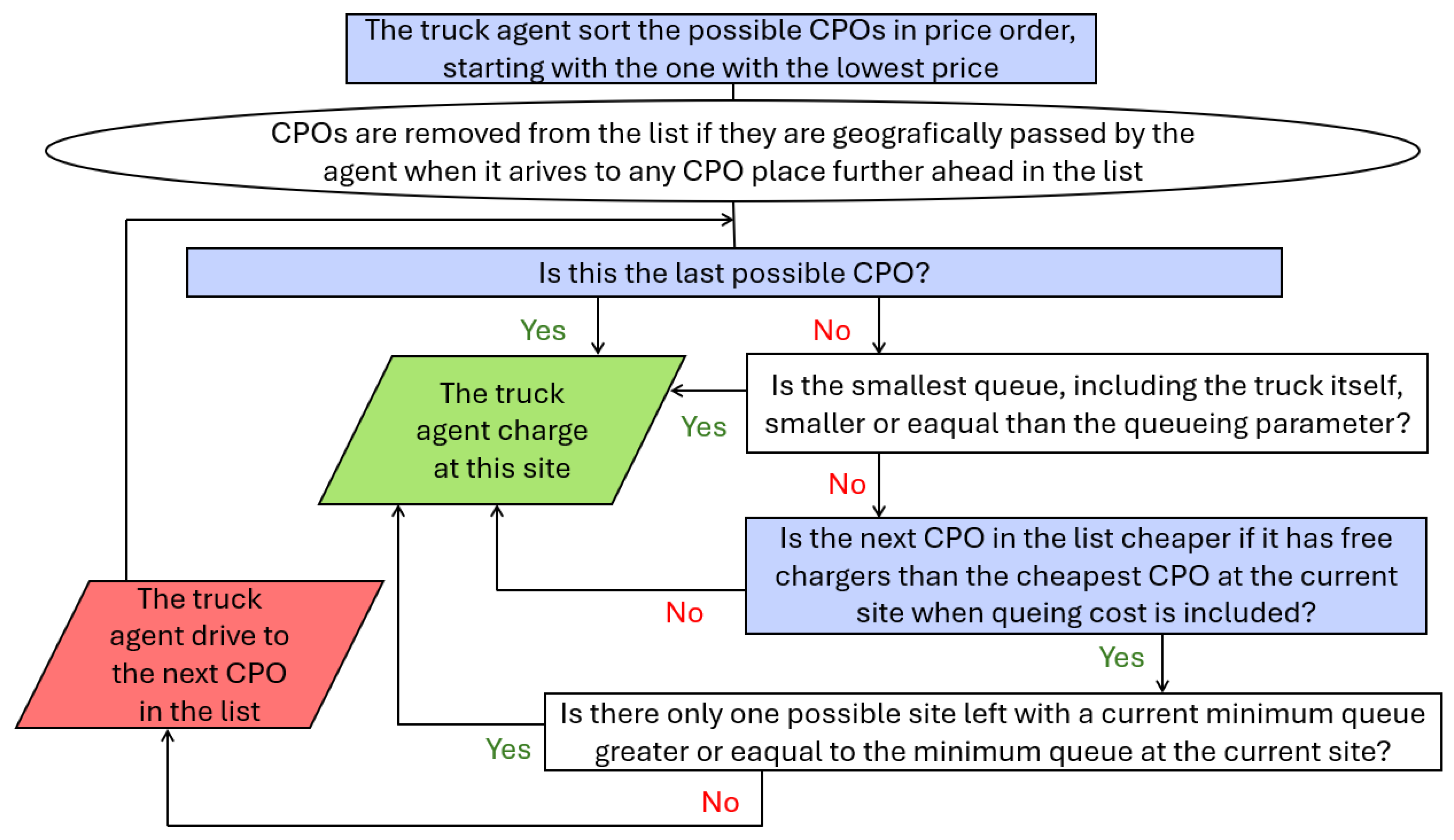
In the first case, where the trucks are sensitive to prices, each truck sorts the possible CPOs in order after the lowest price and aims to charge at the site with the CPO first in this list. This is possible since the trucks in advance of the typical day know the price at each CPO at each hour, their departure time and place, their speed, and the location of the CPOs. For the sake of clarity, CPOs that are passed when a truck is aiming for the CPO associated with the lowest price will be removed from the list as well as the CPOs that are passed if the truck eventually aims for the CPO associated with the second-lowest price and so on—i.e., the truck never turns back in order to find a CPO. This behaviour means that they can drive past a site with free chargers, attracted by a lower price further down the road. When reaching the site of the CPO with the lowest price they will make the decision of whether they should charge there or not. If they do not have the opportunity to drive further, they will charge there (they might be running low in SoC or this is the last site before their destination). However, if they have other possible sites further on, they will stay and charge at this site only if the smallest queue at one of the two CPOs is smaller or equal to the queuing parameter, $q_r$. The queues that affect the decision include the truck that makes the decision. The queuing parameter is set to 0.5 queuing trucks per charger in all the simulations, which corresponds to an expected queuing time of 5 min. If the queue is considered too long, the truck will check the price at the next site in the sorted list—i.e., whether the site with the lowest price further down the road is cheaper than the current CPO when including the queuing cost, as in Subsection 3.4 in Ref. [23], assuming that the CPO at the next site has free chargers. If not, the truck will charge at this site. Otherwise, the truck will continue to the next site, with one exception. The exception is when the truck only has one more possible site to charge at and the current minimum queue at this site is greater than or equal to the smallest queue at the current site. In that case, it is considered too risky to continue to the last possible site. One may truly argue that the queue may turn out to be smaller when the truck arrives at the last site, but it is also possible that the queue is even worse. If a truck charges twice, it first minimises the price for the first charge independent of the next charge, and then minimises the price for the second charge in the same way as described above. In this paper, the behaviour described above is referred to as price-sensitive behaviour. A flowchart of how the price-sensitive trucks select charging sites is given in Figure 4.

In the second case, the trucks are more sensitive to queues. Then the trucks stop and charge at a site if the minimum queue at the site (including the truck itself) is lower than or equal to the queuing parameter, regardless of prices at other sites further down the road. If the minimum queue is considered to be too long, the truck drives to the next site if possible; if this site is the last one, the truck charges at the current site. In this way, the trucks do not drive past CPOs with no or small queues. In this paper, the behaviour described above is referred to as queue-sensitive behaviour. A flowchart of how the queue-sensitive trucks select charging sites is given in Figure 5.

When the truck has selected a site, it selects a CPO in almost the same way as it did in Subsection 3.4 in Ref. [23]. The difference is that the charging time for the trucks (called $T_c$ in Ref. [23]) is set to the mean charging time for the trucks (around 20 min) and that the truck selects the CPO by coin toss in the case that the price, including the expected queuing time, is equal for the two CPOs at the site. As in Ref. [23], the cost for queuing, $C_{c/t}$, is set to 1.5 EUR/min.

It should be noted that trucks in reality likely do not select CPOs in exactly this way; probably, they will weigh both price and queues simultaneously in a more sophisticated way. However, this does not present a problem, as long as the stations obtain more customers due to low prices or small queues. One tricky thing, not just in these simulations but in the future system as well, is that the trucks do not have information about the queues further down the road, since the queue conditions can change with time. A charger booking system could be a solution to this but may also give rise to other drawbacks in the system, for example, extra costs related to the booking system or the fact that missed time slots can possibly cause free chargers and queues simultaneously.

3.6. How CPO Agents Change Their Prices and Number of Chargers

The rules for how CPOs try to adjust their prices and the number of chargers will affect the outcome of the simulation. With one type of behaviour, a specific price level could be profitable, but it might not be profitable under other circumstances. The rules for the CPOs, selected in this paper, are just one setup among infinitely many. The rules have been designed to be both concise and realistic, but most likely, better rules can be created. However, when the rules in this paper were changed as a sensitivity analysis, the outcome differed in, for example, how the price varied over the day, but the greater picture, such as the average charging price and the total number of chargers in the system, was similar.

The CPOs update their prices and number of chargers according to the rules presented below, where each change for the individual CPO occurs with a probability of $P_{prob}={\displaystyle \frac{1}{4}}$ each time a CPO can make changes. The reason that the probability is not close to 1 is that if a CPO tries very often to perform all or almost all changes, one misses the chance to make a change to only one condition that might lead to higher profit, while two simultaneous changes might lead to lower profit. Sometimes, it might be the other way around—that is, simultaneous changes increase profit, but one change alone does not, which is one of the reasons that the probability is not close to zero. The method should make it possible to sometimes not make any changes, sometimes make just one, and sometimes make several. The value of ${\displaystyle \frac{1}{4}}$ was chosen; in addition to giving a sufficient speed of convergence, it is also the same as in Ref. [23], making it suitable for comparison. When price decreases are investigated, the price is never set below the price for electricity plus the profit margin, $P_{marg}$. In this paper, $P_{marg}=0.001$ EUR/kWh in all the simulations.

1.

The CPO adds a charger with probability 0.5. If the CPO does not add a charger, it instead removes one. However, it never removes its last charger.

2.

The CPO compares the charger utilisation with its local competitor (the other CPO at the same site). If there are hours when utilisation is lower than the competitors, the CPO randomly picks one of these hours. With a probability of 0.5, the CPO sets its price for this hour equal to the competitor price, or else to $\Delta C_{epub}$ less than the competitor level, where $\Delta C_{epub}$ is the price change parameter that affects the size in price changes in the simulations.

3.

If there are hours when the CPO has higher or equal prices than the local competitor, the CPO randomly picks one of these hours. With a probability of 0.5, the CPO decreases the price of the hour to the competitor’s level, or else to the local competitor’s price minus $\Delta C_{epub}$.

4.

The CPO randomly selects one hour and decreases the price for this hour by $\Delta C_{epub}$.

5.

The CPO randomly selects one hour and increases the price for this hour by $\Delta C_{epub}$.

6.

If there are hours with queues, the CPO randomly picks one of these hours and increases the price for this hour by $\Delta C_{epub}$, or if it results in a higher price, the CPO increases the price to the local competitor’s price minus $\Delta C_{epub}$.

7.

If there are hours when the CPO has lower or equal prices than the local competitor, the CPO randomly picks one of these hours. With probability 0.5, the CPO increases the price for this hour by $\Delta C_{epub}$ or, if it results in a higher price, to the competitor’s level; otherwise, it increases the price for the hour by $\Delta C_{epub}$ or, if it results in a higher price, to the local competitor’s price minus $\Delta C_{epub}$.

In rules 8 and 9, the price changes are inspired by a neighbouring site. If the CPO is located at the first or last site, there is only one neighbouring site; otherwise, there are two. Which of the two neighbouring sites to compare the price with is decided by a coin toss each time. The CPO can compete for the same trucks with CPOs at a neighbouring site. However, if it is a competition concerning the price, and not for free chargers, the trucks selecting a site will need to compare the present price at the current site it is at with the future price of the other station it will arrive at. The difference in time is the travel time between the sites. When the travel time is rounded to hours, it becomes

$$T_{\Delta S}=\mathrm{round}(\Delta S/v).$$

(7)

It is necessary to round the time for price setting since the price only changes each hour in this model. Consider a station at a site along the road. Suppose a CPO wants to compete with the CPOs at the neighbouring site to its right (closer to Stockholm), for a specific hour at the competing stations. Then, if the CPO lowers the price at time $T_{\Delta S}$ before the specific hour at the competing site, the CPO will attract trucks coming from the left (from Helsingborg). If instead the CPO wants to attract trucks coming from the right, it should lower the price at time $T_{\Delta S}$ after the specific hour. If instead the CPO wants to strengthen its competition with a site to the left, it will be the other way around. This motivates the following rules:

8.

By a coin toss, it is decided if “RandSign” should be −1 or 1. The CPO compares its charger utilisation at all the hours delayed by $\mathrm{RandSign}·T_{\Delta S}$ with the highest utilisation of the two other competing CPOs at the neighbouring site at the ordinary hours. For example, if $\mathrm{RandSign}=1$ and $T_{\Delta S}=2$ h, the utilisation during the first hour at the competitor site is compared with the third hour at the current site, and the utilisation during the second hour at the competitor site is compared with the fourth hour at the current site, and so on. If there are hours when one of the competitors has higher utilisation, the CPO randomly picks one of these hours. Then, by coin toss, the price at the delayed time is either set to the minimum price at the competing site that hour or to $\Delta C_{epub}$ less than the minimum price.

9.

The CPO compares its price at the time delayed by $\mathrm{RandSign}·T_{\Delta S}$ with the highest price of the two other competing CPOs at the neighbouring site at the ordinary time. If there are hours when one of the competitors has higher price, the CPO randomly picks one of these hours. Then, by coin toss, the price at the delayed time is either set to the maximum price at the competing site that hour or to $\Delta C_{epub}$ less than the maximum price.

In this paper, the price change parameter $\Delta C_{epub}$ is set to 0.001 EUR/kWh in all the simulations. This value was previously used in Ref. [23], where this parameter value was found to be suitable. This value also corresponds well to the precision in price in the Swedish charging market these days (0.01 SEK/kWh). The rules are designed to make the CPO agents adjust their prices and number of chargers to improve their profits under competition. Likely, the rules do not perfectly reflect the actual future public fast-charging market, but since the effects on profits of CPOs making changes are always being evaluated, the prices and number of chargers will change as long as such changes are profitable, making CPOs likely to approach a state where it is hard to improve profit—i.e., one has reached the quasi-equilibrium. Thus, the rules for the CPOs do not have to have a perfect design for the quasi-equilibrium to reflect the competitive situation and the market’s response in a good way.

4. Results

In all simulations, except one (Case 4), there are ten charging sites. The first site is located at position 6 km (6 km from Helsingborg) and then the sites are equidistant with 60 km in between each site. The reason for this is that an EU regulation requires at most 60 km between charging stations along the TEN-T core road network [30]. In one case (Case 4), there are instead only three charging sites, located at positions 138 km, 276 km, and 414 km, respectively.

The model results do not seem to be sensitive to the initial conditions, i.e., initial prices and number of chargers. Due to the presence of randomness in how the CPOs update their number of chargers and prices, the same simulation will not give exactly the same results, even with the same initial conditions. However, the greater picture is the same. In Appendix A, the results from the same simulation setup but with two different sets of initial conditions are shown. In this section, the results from four different cases are presented. In Case 1, the trucks are price-sensitive, in Case 2, the trucks are queue-sensitive, in Case 3, some of the update rules for the CPOs are removed, and in Case 4, there are only three charging sites instead of ten. In the following sections, the results will be summarised, interpreted, and corrected for non-modelled variations of the traffic flow throughout the year. In the model, there are many parameters and their values are hopefully representative for the future. Many of the parameter values were the same in all simulations; in these cases, the values are shown in the nomenclature list.

Table 1. Setup for different simulated cases.

Case	Behaviour	Used Rules	Distance Between Stations (km)
1	Price-sensitive	1–9	60
2	Queue-sensitive	1–9	60
3	Price-sensitive	1–7	60
4	Price-sensitive	1–9	138

shows the different settings for the four simulated cases. A sensitivity analysis for the parameter values would have been desirable but was not conducted due to limited computational power.

4.1. Case 1: Price-Sensitive Trucks

In Case 1, there are ten charging sites, and the trucks have price-sensitive behaviour (described in the previous section). The initial number of chargers was set to five for each CPO and the initial price, over the whole day, was set to 0.4 EUR/kWh. The model was run for $3.5\times {10}^4$ iterations. Figure 6 shows how the minimum and maximum prices over the day develop over the iterations for some of the CPOs. The other CPOs have similar prices. Notice that there is only a small difference in price between the lowest and highest price—thus, the price is quite even throughout the day. Also, notice that the highest price is quite low, far below 0.2 EUR/kWh. Figure 7 shows how the price varies over the day for CPO 5 and 6 for the last iteration. Figure 8 shows how the system mean price and the total number of chargers in the system develop over the iterations. The system mean price is in this article calculated by dividing the total charging cost for the trucks with the total amount of energy delivered to the trucks during the typical day and is not the mean value of the 24 hourly prices. As seen from Figure 8, the searched quasi steady state (defined in Ref. [23]) seems to have been reached at the end of the simulation. Therefore, the following result is obtained by averaging over the last 1.5 $\times {10}^4$ iterations. The mean price in the system is found to be 0.113 EUR/kWh, the total number of chargers in the system is 89, the time-utilisation for the chargers in the system is found to be 68% (i.e., the mean charger is used 68 % of the time), the total profit for the CPOs is found to be 7770 EUR/day, the mean queuing time per charge is 8.2 min, and the worst total queuing time for one truck for the typical day was 102 min (the truck might charge twice).

4.2. Case 2: Queue-Sensitive Trucks

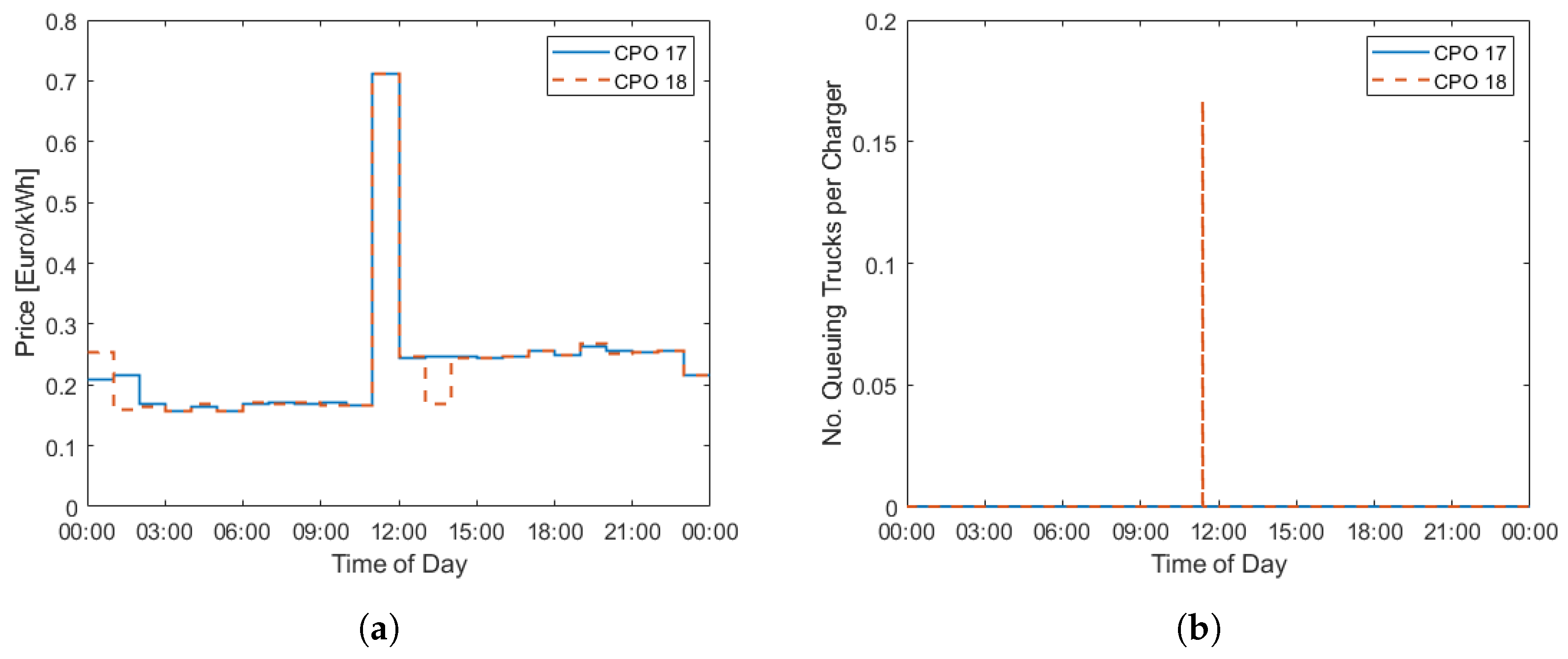
In Case 2, there are ten charging sites, and the trucks have a queue-sensitive behaviour (described in the previous section). The initial number of chargers was set to five for each CPO and the initial price, over the whole day, was set to 0.15 EUR/kWh. The model was run for $5\times {10}^4$ iterations. Figure 9 shows how the minimum and maximum prices over the day develop over the iterations for some of the CPOs. The other CPOs have similar prices.

In this case, there is often a significant difference in price between the lowest and highest level. Figure 9b shows that the highest price for CPOs 17 and 18 tends to be very high and around 0.7 EUR/kWh for the last iteration. However, the price is only that high for one hour while the rest of the hours have significantly lower prices—see Figure 10a, which shows the price throughout the day for the last iteration. Figure 10b shows the number of queuing trucks per charger throughout the day for the last iteration for CPO 17 and CPO 18. Although the queuing conditions could rapidly change with the iterations at a specific site, the figure shows that there is a small lack of chargers during the hour when the price is high. The queue consists of only one truck. Since the price was equal between the two CPOs for this hour, the arriving truck that could not find a charger selected CPO 18 due to its having more chargers than CPO 17. CPO 18 had six chargers this iteration and CPO 17 only had four. Therefore, a truck would choose CPO 18 since that means standing in a queue with fewer queuing trucks per charger. The figure shows that the queue is at lunch time; however, this is not true in general. At other sites, the rush hours can be at other times. As seen from the figure, the queuing problems are small for this site and specific iteration, which is also valid for all the sites during iterations in the quasi-steady state. 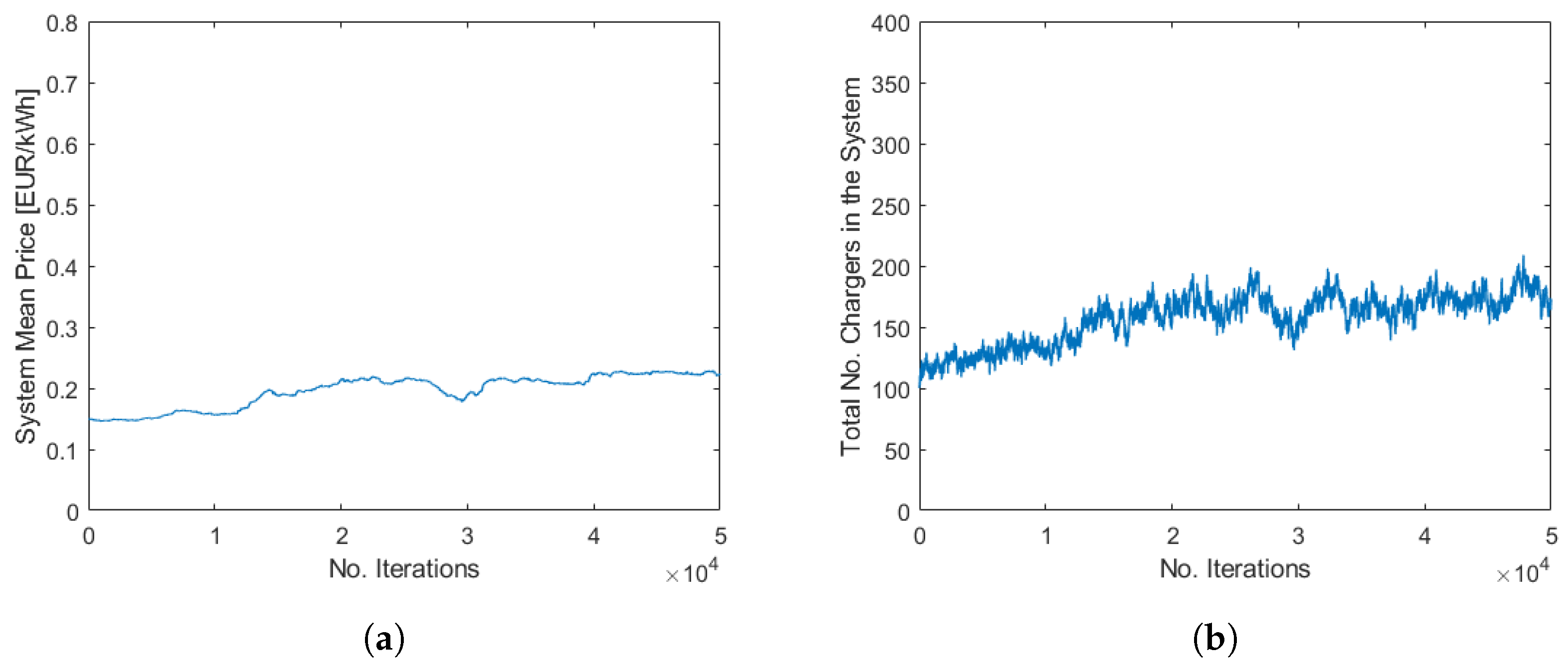Figure 11 shows how the system mean price and the total number of chargers in the system develop over the iterations. As seen from Figure 11, the searched quasi-steady state seems to have been reached by the end of the simulation. Therefore, the following result is averaging over the last 1 $\times {10}^4$ iterations. The mean price in the system is found to be 0.225 EUR/kWh, the total number of chargers in the system is 175, the time utilisation for the chargers in the system is found to be 35%, the total profit for the CPOs is found to be 97,100 EUR/day, the mean queuing time per charge is 0.1 min (6 s) and the worst total queuing time for one truck for the typical day is 21 min (the truck might charge twice).

4.3. Case 3: CPO Without Direct Influence of Neighbouring Sites

In Case 3, there are ten charging sites, and the trucks have a price-sensitive behaviour. The difference from Case 1 is that update rules eight and nine for the CPOs are removed (see Section 3.6). These rules were designed so that the CPOs would try to compete with neighbouring sites. Thus, one may see this case as a simulation without direct influence of neighbouring sites for the CPOs. The initial number of chargers was set to five for each CPO and the initial price, over the whole day, was set to 0.25 EUR/kWh. The model was run for $1.5\times {10}^5$ iterations. 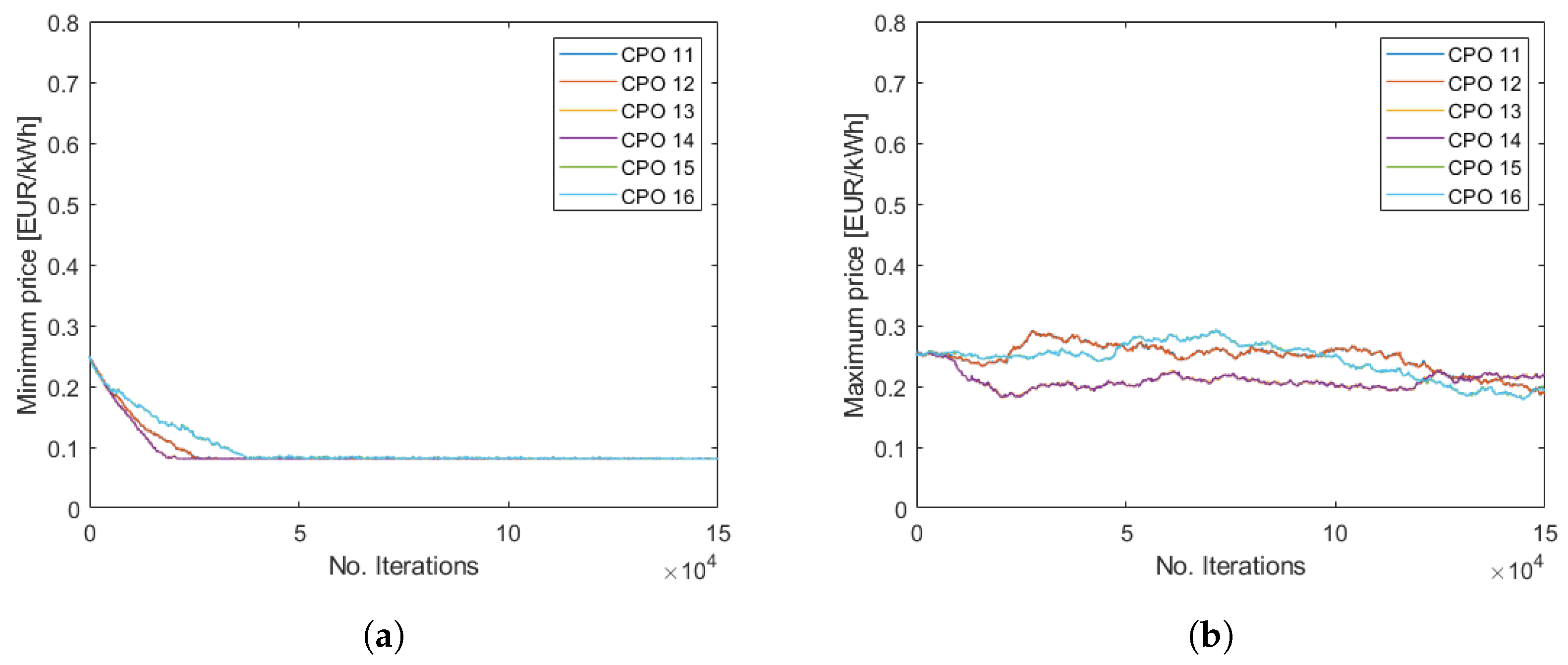Figure 12 shows how the minimum and maximum prices over the day develop over the iterations for some of the CPOs. The other CPOs have similar prices, some with lower peak price. Notice that in this case there is a significant difference in price between the lowest and highest price, and that the lowest price is at the bottom level while the mean price is almost the same as in Case 1. 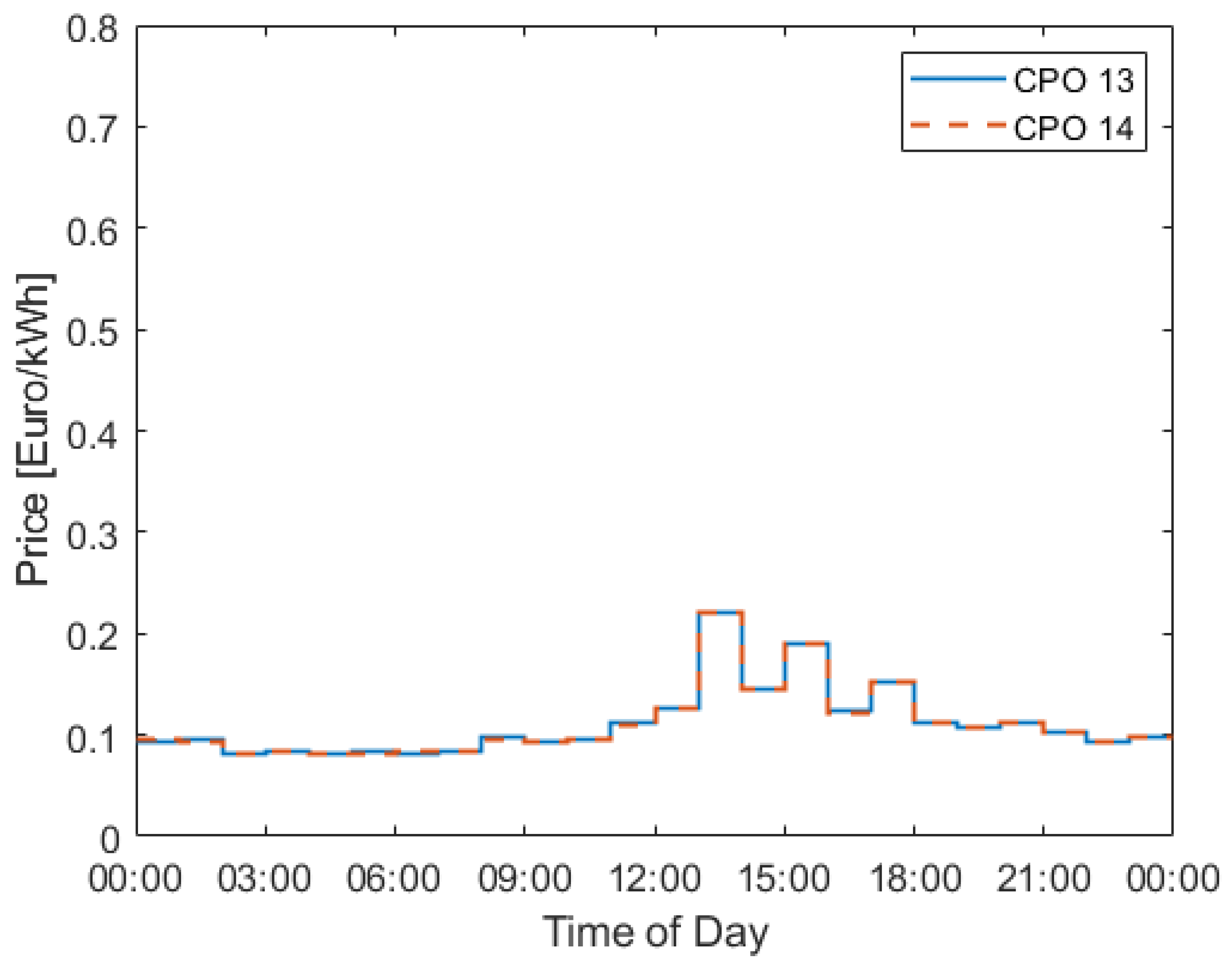Figure 13 shows how the price varies throughout the day for CPO 13 and 14 for the last iteration. Figure 14 shows how the system mean price and the total number of chargers in the system develop over the iterations. As seen from Figure 14 the searched quasi-steady state is reached at the end of the simulation. Therefore, the following result is the result of averaging over the last 1 $\times {10}^4$ iterations. The mean price in the system is found to be 0.111 EUR/kWh, the total number of chargers in the system is 86, the time-utilisation for the chargers in the system is found to be 71%, the total profit for the CPOs is found to be 6660 EUR/day, the mean queuing time per charge is 6.4 min, and the worst total queuing time for one truck for the typical day is 92 min.

4.4. Case 4: Three Charging Sites Only

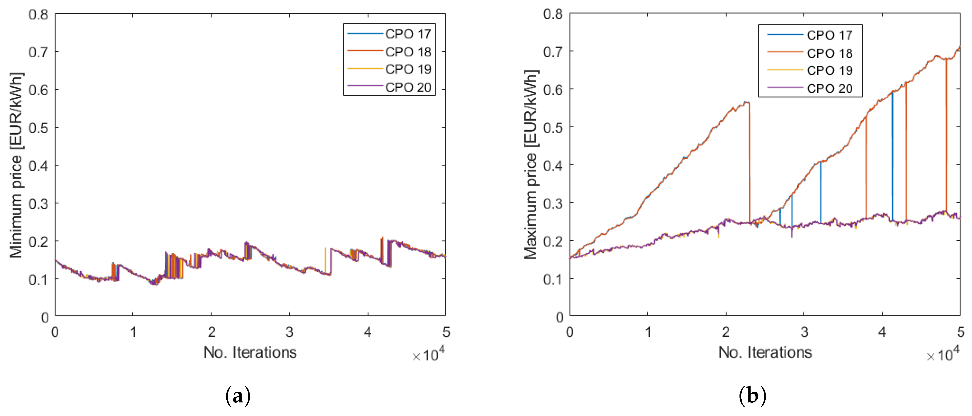
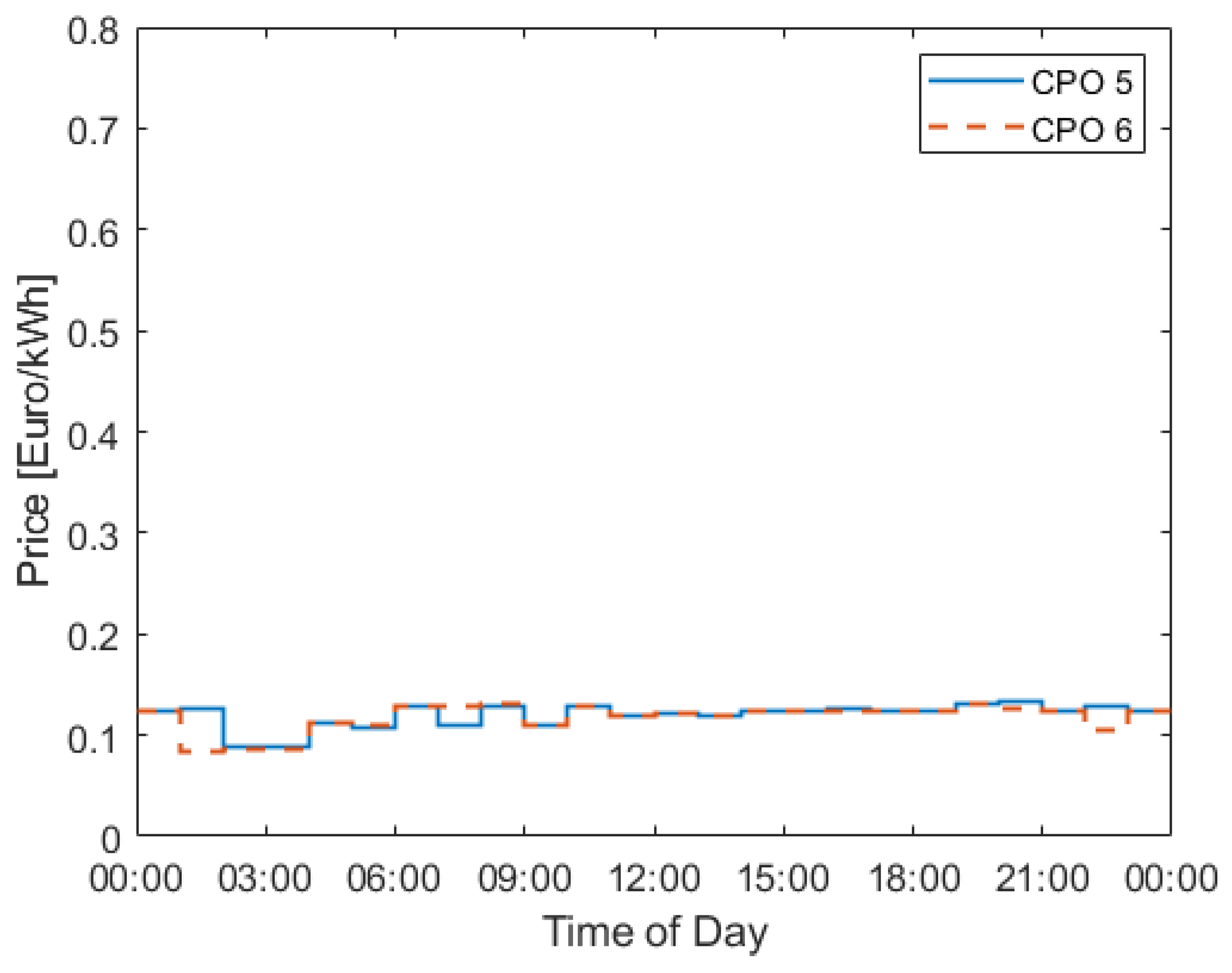
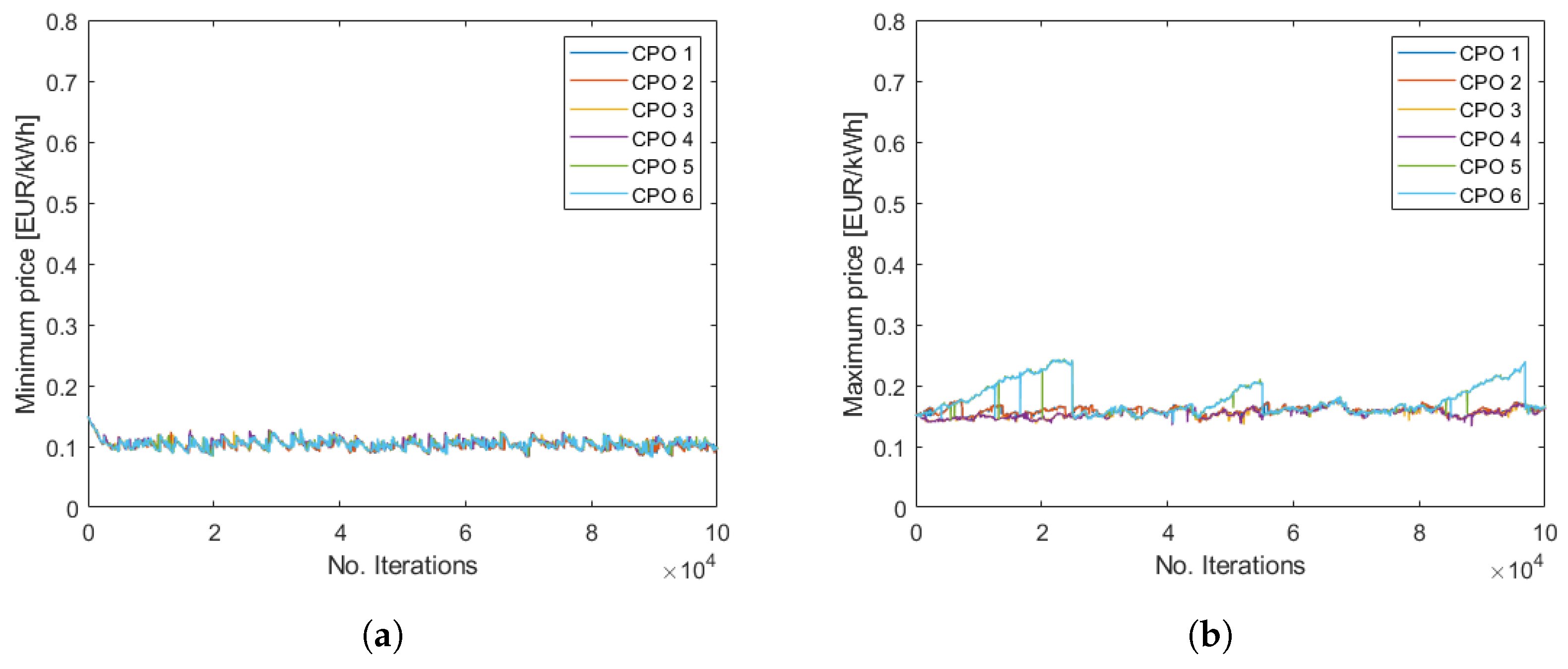
In Case 4, there are three charging sites only and the trucks have price-sensitive behaviour. The initial number of chargers was set to 17 for each CPO and the initial price, over the whole day, was set to 0.15 EUR/kWh. The model was run for $1\times {10}^5$ iterations. Figure 15 shows how the minimum and maximum prices over the day develop over the iterations for all CPOs. The difference in price between the lowest and highest price is, as in Case 1, small. Thus, the price is quite even throughout the day. Also, notice that the highest price is quite low. Figure 16 shows how the system mean price and the total number of chargers in the system develops over the iterations. As seen from Figure 16, the searched quasi-steady state seems to have been reached early in the simulation, but with larger fluctuations compared to Case 1. In Figure 15b, it is noticed that the maximum price for the site with CPO 5 and CPO 6 increases strongly during three periods. But, since the mean price is not affected to a great extent, one may suspect that this just happens for one or a few hours throughout the day. The following results are obtained by averaging over the last 1.5 $\times {10}^4$ iterations. The mean price in the system is found to be 0.135 EUR/kWh, the total number of chargers in the system is 95, the time-utilisation for the chargers in the system is found to be 64%, the total profit for the CPOs is found to be 28,600 EUR/day, the mean queuing time per charge is 1.7 min, and the worst total queuing time for one truck for the typical day is 32 min.

5. Summary and Discussion of the Results

Previously, four cases of competing CPOs and charging trucks were presented. Below, the results are summarized and discussed. An overview is presented in

Table 2. Summarised results.

Case	Mean Price (EUR/kWh)	Mean Queueing Time (min)	Total Number of Chargers (-)	Time Utilisation of Chargers (-)
1	0.113	8.2	89	68%
2	0.225	0.1	175	35%
3	0.111	6.4	86	71%
4	0.135	1.7	95	64%

.

5.1. Summary and Discussion of Case 1

In Case 1, the trucks are clearly price-sensitive and can, in the extreme case, bypass a site with no queue just to charge for 0.001 EUR/kWh less at another site where the queue could be long. This truck behaviour gives rise to a system with very low prices for public fast charging but with few chargers and sometimes severe queues. Unexpected queuing time is, of course, undesirable! In this paper, the indirect queuing cost for the haulier is estimated to 1.5 EUR/min. On average, a charging truck will be queuing for 8.2 min and the mean energy charge at one charge, ${\overline{E}}_{oneCharge}$, is about 230 kWh. With this queuing time, one can find a new average charging price where the queuing time is included:

$$\begin{array}{c}\hfill \mathrm{Mean}\mathrm{price}\mathrm{with}\mathrm{queuing}\mathrm{time}=\mathrm{mean}\mathrm{price}+{\displaystyle \frac{\mathrm{mean}\mathrm{queuing}\mathrm{time}\mathrm{per}\mathrm{charge}·C_{c/t}}{{\overline{E}}_{oneCharge}}}\\ \hfill =0.113\mathrm{EUR}/\mathrm{kWh}+{\displaystyle \frac{8.2\min ·1.5\mathrm{EUR}/\min }{230\mathrm{kWh}}}=0.166\mathrm{EUR}/\mathrm{kWh}.\end{array}$$

(8)

This is clearly a low price for public fast charging, but the large risk for significant queuing is truly a drawback. The authors do not think that the majority of truck drivers will act in this way since it introduces such a large risk of queuing and therefore view this result as an extreme case. The prices are simply too low to make it profitable to build chargers for the peak demand. Also, in this paper, a typical day is simulated but without considering the variation in traffic flow throughout the year. To have a system that is robust against queues, it is necessary to have more chargers than for the typical day. But since it does not seem profitable for the CPOs to build chargers for the peak demand of the typical day, they will probably not build even more chargers to meet an even higher peak demand some days. This means that the queuing conditions will be even worse some of the days but also better some days when the traffic flow is lower. In a system like this, a charger booking system could be a part of the solution. A booking system may help better distribute the trucks over the existing chargers, and could in the best case broaden the peak demand, which could lead to profitable extra charges. However, it will not directly create more chargers, which is required if the number of chargers is too low.

In Case 1, the price is quite even throughout the day and the price is rarely at the lowest level. This result contradicts a result from a previous study [23]. A natural conclusion is that geographically spread CPOs give rise to a more even price structure throughout the day given that the previous study only investigated competing CPOs at one site. But this is only partially true, and the difference could also be explained by the new update rules for the CPOs, which make it possible for them to change prices in greater leaps than was possible in Ref. [23].

5.2. Summary and Discussion of Case 2

In Case 2, the trucks are queue-sensitive but not as price-sensitive as in Case 1. In the extreme case, the trucks could stop at a site with very high prices just because the queues are short or non-existent. This behaviour gives rise to a system with many chargers and almost no queues but with significantly higher prices compared to Case 1. The mean price with the small queuing time included can be found in the same way as in the previous subsection:

$$\begin{array}{c}\hfill \mathrm{Mean}\mathrm{price}\mathrm{with}\mathrm{queuing}\mathrm{time}=\mathrm{mean}\mathrm{price}+{\displaystyle \frac{\mathrm{mean}\mathrm{queuing}\mathrm{time}\mathrm{per}\mathrm{charge}·C_{c/t}}{{\overline{E}}_{oneCharge}}}\\ \hfill =0.225\mathrm{EUR}/\mathrm{kWh}+{\displaystyle \frac{0.1\min ·1.5\mathrm{EUR}/\min }{230\mathrm{kWh}}}=0.226\mathrm{EUR}/\mathrm{kWh}.\end{array}$$

(9)

This is higher than in Case 1 but the price is still reasonable, and there are clearly low queuing problems. In this case, the prices are high enough for the CPOs to profitably meet demand during rush hours. Thus, it seems likely that the CPOs will build enough chargers to resist queues even on days with higher or more uneven charging demand than for the typical day. However, such more uneven demand will require a higher average price to finance the extra chargers. In a coming section, the higher mean price, caused by rare days with higher demand than the typical day, will be estimated.

In Case 2, the price is quite even throughout the day if some hours are excluded, but for some hours, the price can be really high. This has been seen in a previous study [23], where only one site with a constant charging demand each iteration was investigated. Now, when the trucks stop and charge due to the queues being sufficiently small regardless of price, the variation in charging demand at each site is likely lower between the iterations compared to Case 1. In Case 1, all trucks aim for the site with the lowest price for each iteration, which pushes the price to a more even level throughout the day. The authors interpret the above as the geographical spreading of the CPOs, in Case 2, having less impact, and the price picture throughout the day is more like the result in Ref. [23]. We think this indicates that a system where trucks select between sites that are geographically spread will generate more even price pictures throughout the day than if trucks always charge at the same site. However, the price is not at the lowest level large parts of the day as it is in Ref. [23]. The reason for this is that new update rules have been added (number eight and nine), which will be discussed in the next subsection. These update rules make it possible to change the price in leaps, far greater than $\Delta C_{epub}$. In Ref. [23], it is argued that, as soon as the charging demand is a bit lower than the supply, the prices will decrease to a low level during the iterations. This is explained by the fact that a CPO that has a price of $\Delta C_{epub}$ less than its competitors will obtain many more customers. A price increase with the step $\Delta C_{epub}$ is not enough to earn more money from the higher price than what one loses given fewer customers. In this paper, the CPOs can, due to greater leaps, increase the price and still earn more money despite the loss of customers. Now, consider Figure 9a. One notices the same behaviour as in Ref. [23]: the minimum price decreases over the iterations but at some point the price is increased with a large step and then falls again, and so on. In reality, the CPOs will be able to increase the price more than just a small step and we therefore see the new added rules as an improvement in the behaviour of the CPOs.

One may notice that for all the simulations, there seems to be a correlation between the system mean price and the total number of chargers in the system—i.e., when the mean price is low, there are few chargers, and when the mean price is high, there are many chargers. This might be extra clear from the following case: see Figure 11, in particular the small dip in price and number of chargers after about 3 $\times {10}^4$ iterations. This correlation seems natural since the charger utilisation decreases with increasing number of chargers—i.e., the cost for the chargers per delivered kWh increases. Higher prices are therefore demanded to compensate for an increase in the number of chargers.

5.3. Summary and Discussion of Case 3

In Case 3, the trucks are sensitive to price and update rules eight and nine for the CPOs are removed. These rules make it possible for the CPOs to change their prices in large leaps. When they are removed, one notices that the low prices, as in Ref. [23], again are at the lowest level. Also, as in Ref. [23], a larger variation in the price throughout the day appears. So, it seems like the reason that the prices are more even throughout the day in this paper compared to Ref. [23] is not only that the CPOs are dispersed in space but also due to less constraining update rules for the CPOs. However, the greater picture is in many ways quite alike. The mean price and number of chargers are very similar in Case 1 and Case 3. Even if the difference in queuing time is small, the authors admit a bit of confusion; the queuing time in Case 1 is a bit larger than in Case 3 despite the number of chargers being slightly higher in Case 1 compared to Case 3. A possible explanation is that the chargers are a little bit better distributed in the system in Case 3 compared to Case 1. This case can be seen as a sensitivity test for the update rules of the CPOs. This particular test shows that the mean price and queuing time seem much less sensitive than the price picture throughout the day.

5.4. Summary and Discussion of Case 4

In Case 4, the trucks are sensitive to price and there are three charging sites only. Due to the long distance between the sites, fewer trucks can select more than one site, so one may guess that it is not as important if the trucks are sensitive to price or queues. This case leads to a system with low prices and few queuing problems! The mean price is a bit higher than in Case 1 and there are a little bit more chargers as well. However, this is not the main reason for the lower queuing problem compared to Case 1. A result from the literature [21] is that fewer large charging sites better resist queues than many small ones (provided that the total number of chargers are the same). According to the EU Alternative Fuel Infrastructure Regulation [30], the distance between sites should be no more than 60 km along larger roads, as in Cases 1 to 3. There could be benefits associated with more dense charging sites, such as that trucks can avoid detours for charging, but from the results there also seem to be drawbacks. Thus, the results from Case 4 indicate that the minimum distance law could have some negative effects. For Case 4, the mean price with the queuing time included is found in the same way as previously:

$$\begin{array}{c}\hfill \mathrm{Mean}\mathrm{price}\mathrm{with}\mathrm{queuing}\mathrm{time}=\mathrm{mean}\mathrm{price}+{\displaystyle \frac{\mathrm{mean}\mathrm{queuing}\mathrm{time}\mathrm{per}\mathrm{charge}·C_{c/t}}{{\overline{E}}_{oneCharge}}}\\ \hfill =0.135\mathrm{EUR}/\mathrm{kWh}+{\displaystyle \frac{1.7\min ·1.5\mathrm{EUR}/\min }{230\mathrm{kWh}}}=0.146\mathrm{EUR}/\mathrm{kWh},\end{array}$$

(10)

which is truly low despite low queuing problems!

6. Further Analyses of the System with Queue-Sensitive Trucks (Case 2)

The authors think that the results from Case 2 when the trucks are queue-sensitive are of special interest since they can give an upper bound for the mean price for roads with similar conditions as the studied one. Therefore, this section will further investigate Case 2.

6.1. Correction of Mean Price and Charger Utilisation for Non-Modelled Flow Variation Throughout the Year

In the case with queue-sensitive trucks, the prices for fast charging become sufficiently high so the CPOs can meet the peak demand for charging. This makes it likely that they, in reality, would build even more chargers so the system can resist queues even at peak demands higher than the typical day. Since the trucks are willing to pay to avoid queues, the price for public fast charging will now be corrected due to more chargers in the system compared to Case 2. Since the other studied cases resulted in lower mean prices, this value can be seen as an estimate of an upper bound for the mean price for roads with similar conditions as the studied road.

In this study, a typical day representing a weekday was simulated. In reality, there will likely be fewer trucks on the road on weekends and the flow variations throughout the year will be more uneven than the flow of the typical day. Therefore, there is probably a need for more chargers than were found in the simulation and it is likely that the CPOs will lose some income due to lower charging demand on weekends. It is assumed that the CPOs will increase their prices to compensate for this, so the price and charger utilisation will be adjusted to account for the above. This might be carried out in the same way as in Ref. [21], where it is assumed that the charging need over the week is reduced by ${\displaystyle \frac{1}{7}}$ because of lower charging demand on weekends. In the aforementioned study, the number of chargers in the system was increased by 33% to be able to handle increased traffic and unexpected peaks in the charging demand throughout the year. The charging need for the typical day, $E_{tot}$, is $1\times {10}^6$ kWh. The mean price in Case 2 was 0.225 EUR/kWh, so the reduced profit due to weekends can be calculated as follows:

$$\begin{array}{cc}\hfill \mathrm{reduced}\mathrm{profit}\mathrm{due}\mathrm{to}\mathrm{weekends}& ={\displaystyle \frac{1}{7}}·E_{tot}·(0.225\mathrm{EUR}/\mathrm{kWh}-C_e)\hfill \\ \hfill & ={\displaystyle \frac{1}{7}}·\mathrm{1,000,000}\mathrm{kWh}/\mathrm{day}·0.145\mathrm{EUR}/\mathrm{kWh}\hfill \\ & =\mathrm{21,000}\mathrm{EUR}/\mathrm{day}.\hfill \end{array}$$

(11)

Further, the number of chargers in Case 2 was 175, so there is a need for 175 × 0.33 = 58 more 900 kW chargers. Since $C_{ch}=0.32\mathrm{EUR}/\mathrm{kW}$, the extra cost for chargers is found as follows:

$$\mathrm{cost}\mathrm{for}\mathrm{extra}\mathrm{chargers}=58·900\mathrm{kW}·0.32\mathrm{EUR}/\mathrm{kW}/\mathrm{day}=\mathrm{17,000}\mathrm{EUR}/\mathrm{day}.$$

(12)

The two equations above give the total extra income needed to compensate for the non-modelled flow variations over the year:

$$\begin{array}{cc}\hfill \mathrm{total}\mathrm{extra}\mathrm{income}\mathrm{needed}& =\mathrm{reduced}\mathrm{income}\mathrm{due}\mathrm{to}\mathrm{weekends}+\mathrm{cost}\mathrm{for}\mathrm{extra}\mathrm{chargers}\hfill \\ \hfill & =\mathrm{21,000}\mathrm{EUR}/\mathrm{day}+\mathrm{17,000}\mathrm{EUR}/\mathrm{day}\hfill \\ \hfill & =\mathrm{38,000}\mathrm{EUR}/\mathrm{day}.\hfill \end{array}$$

(13)

It is assumed that the profit will be the same with less demand and the extra chargers. Therefore, the charging price has to be corrected. Exactly how this extra cost will be distributed throughout the day will not be discussed in this article, but the new mean price can now be calculated:

$$\mathrm{Mean}\mathrm{price}\mathrm{after}\mathrm{adjustment}=0.225\mathrm{EUR}/\mathrm{kWh}+{\displaystyle \frac{\mathrm{38,000}\mathrm{EUR}/\mathrm{day}}{1·{10}^6\mathrm{kWh}/\mathrm{day}·\frac{6}{7}}}=0.269\mathrm{EUR}/\mathrm{kWh},$$

(14)

where the factor ${\displaystyle \frac{6}{7}}$ corresponds to the reduced charging need on weekends. The extra 58 chargers make it likely that there will be no queues most of the days, and only small queues for days with increased charging demand or when there are unexpected peaks in the traffic flow (maybe with the exception of some days with really extreme charging demand). Even the charger utilisation should be corrected. The time-utilisation was found to be 35% for Case 2. When compensating for the extra chargers, weekends, and the fact that a 900 kW charger on average delivers 700 kW, one obtains the adjusted energy-utilisation:

$$\mathrm{Energy}\text{-}\mathrm{utilisation}\mathrm{after}\mathrm{adjustment}=35\%/1.33·{\displaystyle \frac{6}{7}}·{\displaystyle \frac{700}{900}}=18\%,$$

(15)

which is less than what was found in Ref. [21] (30%), but still fairly good. The reason for the lower value in this study, found for Case 2, is that the chargers are dispersed over more charging sites due to the EU Alternative Fuel Infrastructure Regulation [30]. In reality, queues or higher prices at rush hours will likely make some haulage companies reschedule their trips, a factor not included in this study. However, such behaviour would lead to higher utilisation of the chargers and likely lower average charging prices. The above calculations also show that there is a need for 233 chargers, each with power 900 kW, if all the long-haul trucks that drive along the studied highway are electrified. This is more than what was found in [21] (140 chargers) for the same reason as above.

6.2. Return on Investment for the CPOs

The total profit for all the CPOs for Case 2 was found to be 97,100 EUR/day, which is achieved with 175 chargers plus the extra 58 chargers to resist queues on the days when the peaks in the charging demand are high, as found in the previous subsection. Thus, the total number of chargers is 233. Previously in the literature [5], the lifetime for chargers was assumed to be seven years, and the same assumption will be made in this paper as well. Now, the aim is to find the yearly average return on investment for the CPOs. Let A be the initially invested capital, B the income, and Z the operating expenses over Y years and $A_Y$ the remaining value of the investment after Y years. The yearly average return on investment can be defined as follows:

$$RoI={\left({\displaystyle \frac{A_Y+B-Z}{A}}\right)}^{1/Y}-1.$$

(16)

In order to find this value, the operating expenses for the grid have to be extracted from the cost parameter $C_{ch}$, which is the daily cost for the chargers and grid connection. Recall that $C_{ch}=0.32$ EUR/kW/day. It is assumed that the operating cost for the grid connection corresponds to half of the value of $C_{ch}$ and the rest was the initial investment cost for the chargers. This corresponds well with the previously assumed values in the literature [4]. Thus, the initial investment cost for 233 chargers, each with a power of 900 kW becomes

$$A=233·{\displaystyle \frac{0.32\mathrm{EUR}/\mathrm{kW}/\mathrm{day}}{2}}·900\mathrm{kW}·7\mathrm{year}·365\mathrm{day}/\mathrm{year}=\mathrm{85,700,000}\mathrm{EUR}.$$

(17)

Further, the profit from Case 2 can be used to find $B-Z$ since

$$\begin{array}{cc}\hfill & \mathrm{97,100}\mathrm{EUR}/\mathrm{day}·7\mathrm{year}·365\mathrm{day}/\mathrm{year}=B-Z-A\hfill \\ \hfill & \Rightarrow B-Z=\mathrm{97,100}\mathrm{EUR}/\mathrm{day}·7\mathrm{year}·365\mathrm{day}/\mathrm{year}+A\hfill \\ \hfill & =\mathrm{334,000,000}\mathrm{EUR}.\hfill \end{array}$$

(18)

Since the chargers are assumed to have a lifetime of 7 years, one may find $RoI$ by inserting $Y=$ 7 year and $A_Y=$ 0 EUR in Equation (16):

$$RoI={\left({\displaystyle \frac{\mathrm{334,000,000}\mathrm{EUR}}{\mathrm{85,700,000}\mathrm{EUR}}}\right)}^{1/7}-1=0.21,$$

(19)

which should be interpreted as the invested capital returning 21% interest every year. This seems very profitable for the CPO. In reality, the competition between the CPOs might be stronger, which could lower this value. In any case, this calculation shows that the prices, low queuing problems, and robustness against peaks in charging demand for Case 2 are not achieved at the expense of the profitability of the CPOs. Thus, the authors see the mean price, 0.27 EUR/kWh, found for Case 2 as an upper bound for the price of public fast charging in a system with similar traffic as the selected highway. The same calculation for Case 1, but without extra chargers for high charging peaks, gives $RoI=7\%$. Thus, truck charging behaviour seems to have a great impact on the possible profit of CPOs.

7. Discussion, Limitations of the Study, and Further Developments

In this paper, the interactions between competing CPOs and charging battery electric trucks along a large highway in Sweden are simulated with an agent-based model. The authors view the assumptions and the core rules determining how the agents act as realistic. The trucks want to charge for a low price and at the same time avoid long queues, and the CPOs aim to increase their profits. The two investigated charging behaviours, price and queue sensitivity, are a bit extreme, and the results for these two behaviours could therefore be seen as boundaries for future prices and queues. The CPOs change prices and the number of chargers to test how to increase their profits, but their search space is limited by the update rules. The authors consider the used rules to be sufficient but truly believe that better rules (or methods) are possible.

In the model, many assumptions are made that could impact the results. For example, in this paper, the electricity price is set to be constant at 0.08 EUR/kWh. If this value were increased, it would increase the charging price in the results, or if it were decreased, the charging price would decrease. If the electricity price varied throughout the day, the charging price would likely vary in a similar way, but it would possibly also change the queuing conditions at different CPOs at different times. Another model limitation is that only two extreme behaviours (queue and price sensitivity) for the trucks are studied. These two cases are of special interest since they provide upper and lower bound for prices and queues. However, more realistically, the trucks will behave somewhere in between these two ways of behaving, and different trucks will behave in different ways. The same goes for the CPOs; different CPOs could set prices and the number of chargers according to different rules or even according to different methods. Also, some CPOs could cooperate. If this could be modelled in a way that agrees with the behaviour of future battery electric trucks and CPOs, the mean price for public fast charging and the mean queuing time along with daily price variations could be given with higher precision than is provided in this paper; this could serve as a topic for future studies. One more suggestion for future studies is to implement a memory capacity for the CPOs and possibly even for the trucks so that their decisions can improve by learning.

The model is quite computationally heavy, and each simulation requires a couple of days of running time on an ordinary computer. The long computational time limits the possibility of different sensitivity analyses and also large-scale use, like simulating the fast-charging market in a whole country with much truck traffic. Even though large-scale use never was the aim of this paper, the authors think that their core method could be suitable for large-scale use if the algorithm is efficiently implemented in a high-performance computing language and is run on a powerful computer, especially if the update rules for the CPOs are in some way refined so that the simulations converge faster.

8. Conclusions

Since a complex system has been studied using a simplified model, the results of this paper should be seen as indications and estimates and not absolute truths. The model could be made simpler, with the risk of failing to represent important mechanisms, or more complicated, with no guarantee that one would obtain more accurate results. Despite this, the study has produced some interesting conclusions for modelling a future public fast-charging market for long-haul battery-electric trucks along roads with similar charging demand as the studied one.

1.

The results indicate that the price throughout the day will be less varied and a bit higher at off-peak hours compared to predictions from our previous research [23]. The reason is likely that the CPOs are geographically spread out and that they can update their prices in greater leaps as compared to the previous study. Geographically spread CPOs and a broader search space for new prices are realistic properties for a future fast-charging market.

2.

The collective behaviour of the haulage companies can influence the price level, queuing conditions, and profitability of the CPOs significantly. Price-sensitive trucks can result in a system with low prices and queuing problems, while queue-sensitive trucks seem to lead to a system with higher prices but almost no queuing problems. The CPOs seem to be more profitable if the trucks are sensitive to queues compared with price-sensitive behaviour.

3.

The mean charging price is predicted to be around 0.27 EUR/kWh or lower in a system with small or non-existent queuing problems. In this case, the energy-utilisation of the chargers is estimated to be 18%. To achieve this, for the selected highway between Helsingborg and Stockholm in Sweden, 233 chargers, each with 900 kW power, is estimated to be required for a full electrification of the long-haul truck fleet.

4.

In a system with a really low mean price for public fast charging, such as 0.113 EUR/kWh found in Case 1, the CPOs will likely not build chargers to meet the peak demand, which will result in queuing problems. The mean queuing time per charge in Case 1 was found to be slightly more than 8 min.

5.

The system seems to have potential to be more cost-efficient with less dense charging sites along the highway. But because the EU Alternative Fuel Infrastructure Regulation [30] demands charging stations to be placed at least every 60th km, the design used in Case 3 is not possible even if it seems promising. Possibly, well-intentioned laws and restrictions can have unexpected negative consequences.

What is important, but not included in this paper, is that higher prices or the risk of queues at rush hours could drive some of the haulage companies to reschedule their trips. This will lead to higher utilisation of the public fast chargers and likely even lower charging prices. The results from Case 2 seem promising and could consequently be even better with more even charging demand. The results from this paper indicate that the market has potential to provide a well-functioning system on its own in the case of full electrification. A message to policy-makers is therefore that regulations and subsidies will likely not be required in the long run.