DTCformer: A Temporal Convolution-Enhanced Autoformer with DILATE Loss for Photovoltaic Power Forecasting

Abstract

Photovoltaic power forecasting plays a crucial role in the integration of renewable energy into the power grid. However, existing methods suffer from issues such as cumulative multi-step prediction errors and the limitations of traditional evaluation metrics (e.g., MSE, MAE). To address these challenges, this study introduces DTCformer, a generative forecasting model based on Autoformer. The proposed model integrates a Temporal Convolution Feedforward Network module and a Variable Selection Embedding module, effectively capturing inter-variable dependencies and temporal periodicity. Furthermore, it incorporates the DILATE loss function, which significantly enhances both forecasting accuracy and robustness. Experimental results on publicly available datasets demonstrate that DTCformer surpasses mainstream models, improving overall performance metrics (DILATE values) by 5.0–42.3% in 24 h, 48 h, and 72 h forecasting tasks.

1. Introduction

As a core component of the global energy transition, photovoltaic (PV) power generation capacity has exhibited exponential growth in recent years [1]. Against this backdrop, high-accuracy PV power forecasting has emerged as a critical research focus in smart grid technologies, directly impacting the safety and economic efficiency of power system dispatching [2], and facilitating high-penetration renewable energy integration [3]. As a quintessential time-series forecasting application, PV power forecasting plays a crucial role in maintaining grid stability [4].

However, due to the inherent intermittency and volatility of PV output, its time-series data typically exhibit complex spatiotemporal dependencies, multi-periodic patterns (e.g., diurnal and seasonal cycles), and non-stationarity [5]. These distinctive characteristics impose substantial challenges on conventional forecasting methods and motivate the development of advanced machine learning and deep learning approaches.

Driven by the increasing scale and complexity of renewable energy data, deep learning techniques [6,7,8] have gradually supplanted traditional statistical [9,10] and machine learning models [11]. Recent Transformer-based architectures [12,13,14,15], such as Informer [12] and Autoformer [14], have demonstrated superior performance in handling long-sequence forecasting by leveraging attention mechanisms and time-series decomposition strategies. Despite these advancements, PV power forecasting still faces two critical challenges: (1) the cumulative error problem in multi-step prediction, and (2) the limitations of conventional evaluation metrics that inadequately reflect the temporal structure and correlation of forecasts.

In response to these challenges, this study proposes DTCformer, a novel Transformer-based framework that systematically integrates multi-scale temporal feature extraction and introduces a dual-perspective evaluation framework. The principal contributions of this study are summarized as follows:

(1)

Architectural innovation: We develop the DTCformer framework through systematic integration of core structural components from TCNformer and Autoformer, significantly optimizing temporal feature extraction capabilities.

(2)

Enhanced feature extraction: A temporal convolutional feedforward optimization module is specifically designed to substantially improve the time-series feature extraction performance of the encoder–decoder structure.

(3)

Comprehensive evaluation framework: We construct a dual-perspective evaluation system incorporating DILATE loss function, dynamic time warping (DTW), and the Time Distortion Index (TDI), which provides quantitative assessment of prediction results from both morphological similarity and temporal alignment perspectives, thereby improving prediction accuracy and robustness.

2. Related Work

PV power forecasting methods can be broadly classified into four categories: physical models, statistical approaches, traditional machine learning algorithms, and deep learning techniques. Each category demonstrates unique characteristics in terms of prediction accuracy and scenario suitability.

Physical models establish deterministic relationships between meteorological parameters and power generation outputs, achieving high accuracy under stable weather conditions. However, their performance deteriorates under abrupt meteorological changes [16]. Representative methods include numerical weather prediction (NWP) systems [17], Total Sky Imager (TSI) technologies [18], and satellite image-based forecasting [19]. Model complexity often scales with the number of input variables, and accuracy is constrained by the spatiotemporal resolution of meteorological inputs.

Statistical approaches frame PV power prediction as a time-series analysis problem. Early studies extensively employed Autoregressive Moving Average (ARMA) models and their variants. For instance, Benmouiza et al. [20] applied ARMA for solar irradiance forecasting, while Mahalingam et al. [21] extended this approach to multi-year horizons. However, these models struggle to capture nonlinear dynamics, leading to significant error accumulation under unstable conditions.

Traditional machine learning methods, such as Support Vector Regression (SVR) [22] and K-nearest neighbors (KNN) [23], have demonstrated strong nonlinear modeling capabilities and noise robustness. A comparative study by Zaguras et al. [24] showed that SVR outperforms conventional linear models and artificial neural networks in terms of root mean square error (RMSE).

Deep learning techniques have revolutionized PV forecasting by enabling automatic feature extraction and multi-scale temporal modeling. Recurrent neural networks (RNNs) and their variants, such as Long Short-Term Memory (LSTM) [25,26] and Gated Recurrent Unit (GRU) [27,28,29], capture complex temporal dependencies. Furthermore, hybrid models like CNN-LSTM integrate spatiotemporal features to enhance prediction accuracy [30]. Transformer-based architectures have recently demonstrated state-of-the-art performance in long-sequence forecasting tasks [12], although challenges remain regarding multi-timescale modeling and real-time adaptability.

3. Preliminary

3.1. Time-Series Decomposition

Time-series decomposition, which separates a series into components such as trend, seasonality, and residuals [31], is widely used to reveal underlying patterns and enhance forecasting accuracy. While conventional decomposition methods typically serve as static preprocessing steps applied to historical data, they often fail to dynamically capture evolving patterns and complex interdependencies in long sequences. To address these limitations, recent forecasting models, notably Transformer-based architectures like Autoformer [14], incorporate learnable decomposition modules that adaptively extract temporal structures during training. Building upon this idea, the proposed DTCformer framework further integrates a temporal convolutional optimization module to enhance multi-scale feature extraction and improve the modeling of dynamic temporal dependencies.

3.2. AutoCorrelation

The AutoCorrelation mechanism (·), inherited from the Autoformer model, differs from the traditional attention mechanism by extracting features extraction at the sequence level instead of at individual time steps. The AutoCorrelation function, is denoted as:

$$\begin{array}{c}\hfill R_{xx}\left(\tau \right)=\underset{L\to \infty }{lim}{\displaystyle \frac{1}{L}}\sum _{t=1}^L{X}_t{X}_{t-\tau }\end{array}$$

(1)

In Equation (1), $R_{xx}\left(\tau \right)$ denotes the autocorrelation of the time series, where $X_t$ is the original sequence, $X_{t-\tau }$ is its lagged version, $\tau$ is the time delay, and L represents the sequence length.

$$\begin{array}{c}\hfill {\tau }_1,\cdots ,{\tau }_k=\underset{\tau \in \{1,\cdots ,L\}}{argTopk}\left({\mathrm{R}}_{Q,K}\left(\tau \right)\right)\end{array}$$

(2)

$$\begin{array}{c}\hfill {\widehat{R}}_{Q,K}\left({\tau }_1\right),\cdots ,{\widehat{R}}_{Q,K}\left({\tau }_k\right)=SoftMax\left(R_{Q,K}\left({\tau }_1\right),\cdots ,R_{Q,K}\left({\tau }_k\right)\right)\end{array}$$

(3)

$$\begin{array}{c}\hfill AutoCorrelation(Q,K,V)=\sum _{i=1}^{k}Roll\left(V,{\tau }_i\right){\widehat{R}}_{Q,K}\left({\tau }_i\right)\end{array}$$

(4)

In Equations (1)–(4), the function $argTopk(·)$ selects the k time delays with the highest autocorrelation scores $R_{Q,K}\left(\tau \right)$. The value of k is determined by $k=\lfloor c\times logL\rfloor$, where c is a tunable hyperparameter, typically set to 1. Here, $R_{Q,K}$ denotes the autocorrelation between the query sequence Q and the key sequence K. The attention weights ${\widehat{R}}_{Q,K}\left({\tau }_1\right),\dots ,{\widehat{R}}_{Q,K}\left({\tau }_k\right)$ are obtained via a SoftMax operation over the selected autocorrelation values. The $Roll(V,{\tau }_i)$ operation cyclically shifts the value sequence V by a lag ${\tau }_i$, aligning it with the corresponding autocorrelation weight. This mechanism enables the model to capture long-term dependencies by focusing on the most correlated time shifts.

3.3. DILATE Loss

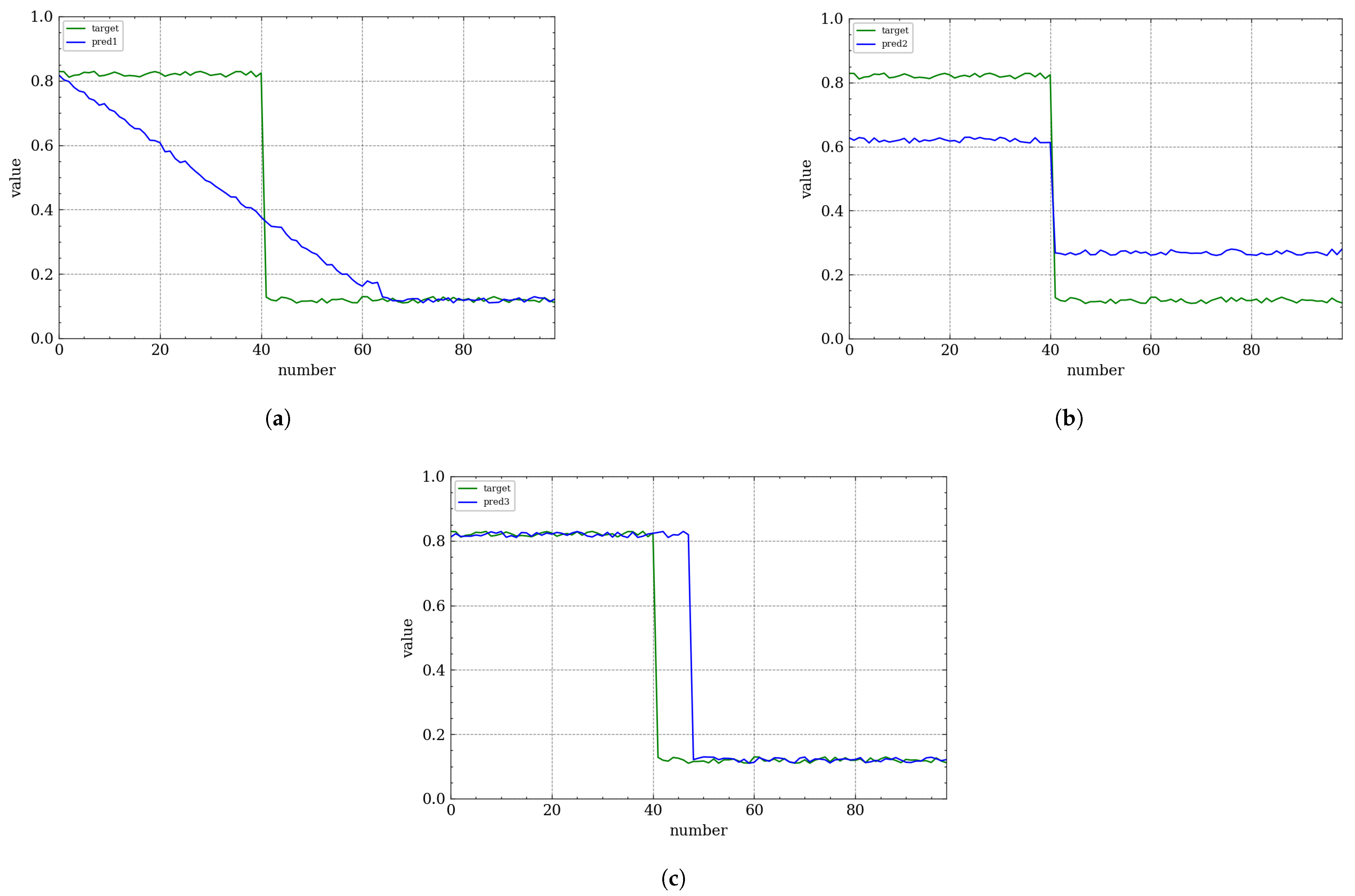
In modern deep learning-based forecasting frameworks, most approaches primarily utilize mean squared error (MSE) or its variants, such as MAE and mean absolute percentage error (MAPE), as their core loss functions. However, in long-term time-series forecasting, relying solely on MSE-based loss functions is inadequate for capturing complex temporal dynamics. This limitation is empirically demonstrated through a comparative case study in Figure 1.

Consider a function prediction task where the ground truth is represented by the blue trajectory. The three subfigures illustrate different prediction outcomes, each exhibiting distinct characteristics. Despite having comparable MSE values relative to the ground truth, each prediction suffers from specific deficiencies in temporal alignment and morphological accuracy.

To overcome these limitations, we introduce DILATE (Distortion Loss Including Shape and Time Errors) [32], a comprehensive loss function tailored for non-stationary time-series prediction. Designed specifically for deep neural networks, DILATE optimizes long-term forecasting by explicitly decomposing prediction errors into two key components: shape distortion and temporal misalignment, each associated with a dedicated penalty term. Empirical studies [33] demonstrate that models trained with DILATE outperform MSE-based approaches, particularly in terms of shape preservation and temporal alignment metrics. Moreover, these models maintain competitive performance on traditional MSE metrics, highlighting DILATE’s versatility across various network architectures. Notably, DILATE enables models to surpass state-of-the-art methods in multi-step non-stationary predictions by achieving superior accuracy in both morphological and temporal aspects.

The DILATE function is calculated as follows:

$$\begin{array}{c}\hfill L_{DILATE}(x,y)=\alpha L_{shape}(x,y)+(1-\alpha )L_{temporal}(x,y)\end{array}$$

(5)

In Equation (5), $L_{shape}$ represents the shape loss, computed using the DTW loss function, which is defined as

$$\begin{array}{c}\hfill L_{\mathrm{shape}}(x,y)={\mathrm{DTW}}_{\gamma }(x,y):=-\gamma log\left(\sum _{\Delta \in {\mathbb{A}}_{k,k}}exp\left(-{\displaystyle \frac{\langle \mathbf{A},\Delta (x,y)\rangle }{\gamma }}\right)\right)\end{array}$$

(6)

In Equation (6), $\Delta (x,y)={\left[\delta (x_i^h,y_i^j)\right]}_{h,j}$ denotes the cost matrix, where $\delta$ represents the distance metric (e.g., Euclidean distance). The smooth minimum operator, defined as ${min}_{\gamma }(a_1,\cdots ,a_n)=-\gamma log\left({\sum }_{A\in A_{k,k}}exp(-a_i/\gamma )\right)$, with $\gamma >0$, is employed to ensure differentiability of the DTW computation.

The temporal loss is defined as:

$$\begin{array}{c}\hfill L_{\mathrm{temporal}}(x,y)={\mathrm{TDI}}_{\gamma }(x,y):={\displaystyle \frac{1}{Z}}\sum _{\Delta \in A_{k,k}}\langle \mathbf{A},\Omega \rangle exp\left(-{\displaystyle \frac{\langle \mathbf{A},\Delta (x,y)\rangle }{\gamma }}\right)\end{array}$$

(7)

In Equation (7), $L_{\mathrm{temporal}}$ represents the time loss, computed using the TDI (Temporal Distortion Index) loss function. The penalty matrix $\Omega \in {\mathbb{R}}^{k\times k}$ systematically accounts for positional mismatches $(h\ne j)$ between temporal indices $x_i^h$ and $y_i^h$. The elements of $\Omega$ are mathematically defined as $\Omega (h,j)={\displaystyle \frac{1}{k^2}}·{(h-j)}^2$, which applies a quadratic penalty for temporal index deviations, scaled inversely with the square of the sequence-length parameter k.

3.4. Temporal Convolutional Network Module

The Temporal Convolutional Network (TCN) is a specialized convolutional architecture designed for temporal sequence modeling. By integrating structural components from RNNs and convolutional neural networks (CNNs), TCN achieves superior empirical performance across various temporal prediction tasks compared to conventional recurrent architectures. A key advantage of TCN lies in its ability to preserve long-range temporal dependencies while maintaining greater computational efficiency than traditional sequence models. This efficiency stems from its dilated causal convolution layers, which systematically capture multi-scale temporal patterns by exponentially expanding receptive fields. Additionally, TCN incorporates residual connections and gating mechanisms, akin to advanced feedforward architectures, allowing for the simultaneous extraction of both linear and nonlinear temporal features through hierarchical feature abstraction.

4. Methodology

The TCN model employs a depthwise-separable causal dilated convolutional architecture, which effectively captures multi-scale temporal features through hierarchical dilation rates and alleviates the vanishing gradient problem in deep networks via a distinctive residual connection design. As a result, TCNformer demonstrates high predictive accuracy and mitigates error accumulation in short-term forecasting tasks. However, its performance still encounters limitations in long-term forecasting scenarios. Given that PV power data are sampled at 15 min intervals, forecasting 24 to 72 h ahead corresponds to a long-term series forecasting (LSTF) task involving 96 to 288 time steps. In this domain, Autoformer has exhibited outstanding modeling capabilities and predictive performance in practical engineering applications [12]. Motivated by these observations, this study proposes the DTCformer model based on a deep decomposition architecture, which integrates the short-term modeling strengths of TCN with the long-term forecasting capabilities of Autoformer to enhance overall predictive accuracy and stability. Specifically, DTCformer leverages TCN’s advantages in capturing short-term local fluctuations and Autoformer’s capabilities in modeling long-term periodic trends via sequence decomposition and AutoCorrelation mechanisms. By combining the short-term modeling strength of TCNformer with the long-term forecasting ability of Autoformer, DTCformer aims to enhance overall predictive accuracy and robustness. The overall architecture of DTCformer is illustrated in Figure 2. The model comprises three main components: the Variable Selection Embedding (VSE) module, the encoder, and the decoder. Within both the encoder and decoder, additional sub-modules are incorporated, including the AutoCorrelation mechanism, the Series Decomposition module, and the Temporal Convolution Feedforward Network (TCNForward).

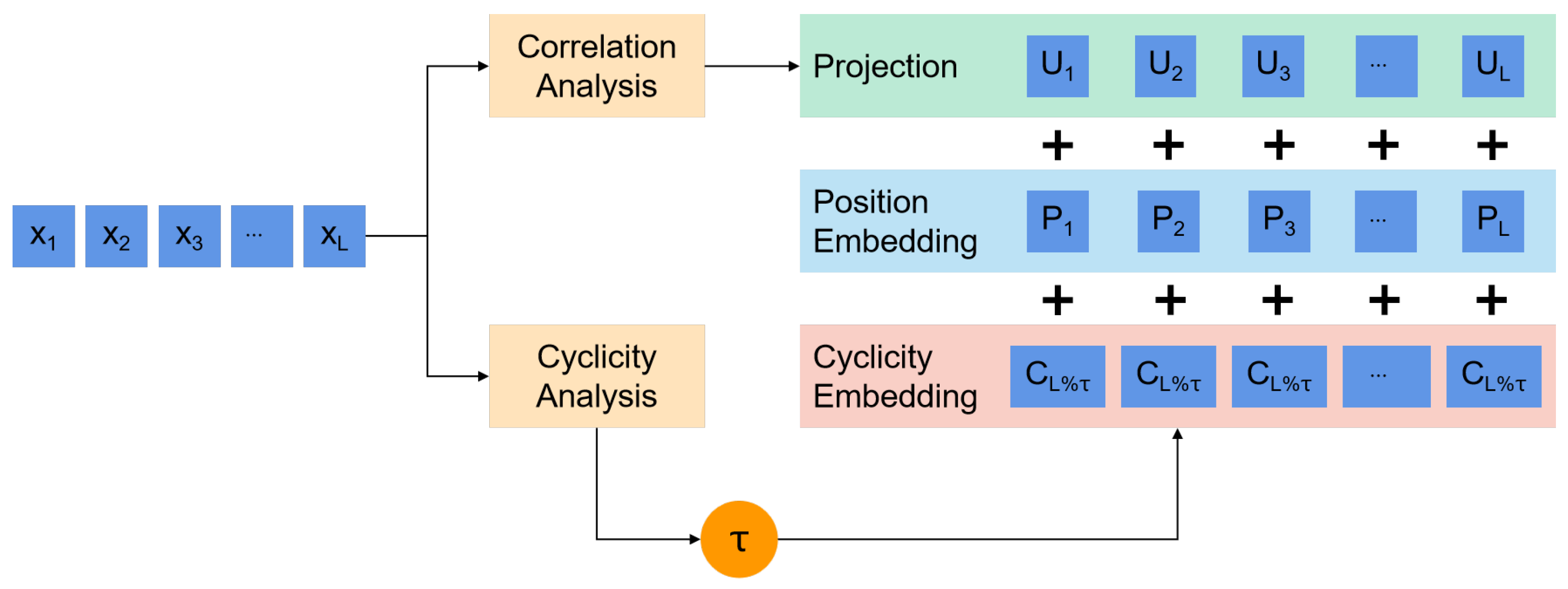
4.1. Variable Selection Embedding Module

The structure of the VSE module is depicted in Figure 3.

The Variable Selection Embedding module is designed based on the Variable Selection module and the Long-Short Term Feature Extraction module in TCNformer. However, given the AutoCorrelation mechanism in the Autoformer model, which excels at multi-scale temporal feature extraction, only the periodic embedding units from the Long-Short Term Feature Extraction module are incorporated. This module leverages periodicity and correlation for variable selection. After selecting the relevant variables, it applies periodic embedding in conjunction with the corresponding static variables. The calculation is formulated as follows:

$$\begin{array}{c}\hfill X=VSE(input,data)\end{array}$$

(8)

In Equation (8), the $\mathrm{input}\in {\mathbb{R}}^{I\times n},\mathrm{and}\mathrm{data}\in {\mathbb{R}}^{B\times n},\mathrm{X}\in {\mathbb{R}}^{I\times d_{model}}$ represent the preprocessed input sequence, the original data, and the input sequence after variable selection embedding, respectively.

Following the Variable Selection Embedding module, an initialization operation for sequence decomposition is applied to the input sequence to capture complex temporal patterns in long-term prediction scenarios. This process divides the input sequence into trend and seasonal components, formulated as follows:

$$\begin{array}{c}\hfill X_t=\mathrm{AvgPool}\left(\mathrm{Padding}\left(X\right)\right)\end{array}$$

(9)

$$\begin{array}{c}\hfill X_s=X-X_t\end{array}$$

(10)

In Equations (9) and (10), $X_s,X_t\in {\mathbb{R}}^{I\times d_{model}}$ correspond to the trend component and the seasonal component, respectively. We employ AvgPool(·) as the moving average and apply padding operations to preserve the constant length of the sequence. This paper utilizes $X_s,X_t=\mathrm{SeriesDecomp}$ to summarize the aforementioned align.

As a decompositional structure, the decoder primarily processes two components: the seasonal component and the trend-cyclic component. Before being passed to the encoder, the input sequence undergoes an initialization operation, formulated as follows:

$$\begin{array}{c}\hfill X_{des}=Concat(X_{ens},X_0)\end{array}$$

(11)

$$\begin{array}{c}\hfill X_{det}=Concat(X_{ent},X_{Mean})\end{array}$$

(12)

where $X_{des}$ represents the seasonal input after concatenation, and $X_{det}$ represents the trend-cyclic input after concatenation. This initialization operation ensures that both seasonal and trend-cyclic components are effectively integrated before encoding, enhancing the model’s ability to capture complex temporal dependencies.

4.2. Encoder

Similar to the encoder structure in Autoformer, the encoder in the DTCformer network is designed to model the seasonal component exclusively. The output of the encoder consists of past seasonal information, which serves as cross-information to assist the decoder in improving the prediction accuracy.

$$\begin{array}{c}\hfill S_{en}^{l,1},\_=\mathrm{SeriesDecomp}\left(\mathrm{AutoCorrelation}\left(X_{en}^{l-1}\right)+X_{en}^{l-1}\right)\end{array}$$

(13)

$$\begin{array}{c}\hfill S_{en}^{l,2},\_=\mathrm{SeriesDecomp}\left(\mathrm{TCNForward}\left(S_{en}^{l,1}\right)+S_{en}^{l,1}\right)\end{array}$$

(14)

In the DTCformer architecture, we introduce a novel TCNForward module, which replaces the conventional feedforward module typically employed in Transformer models. In traditional Transformer-based models, the feedforward module is responsible for deepening the network and facilitating the extraction of more intricate features. However, our investigation suggests that the potential of the feedforward module for enhancing time-series forecasting has not been fully exploited. Although the AutoCorrelation mechanism effectively captures long-range temporal relationships within sequences, it does not account for the temporal dynamics between individual data points. To address this limitation, we integrate a TCN, specifically optimized for time-series prediction. This leads to the development of the TCNForward module, enabling the DTCformer model to extract temporal features both at the sequence level and at the granularity of individual time steps. This dual-level feature extraction provides a more comprehensive understanding of the underlying temporal patterns in the data. The architectural structure of the TCNForward module used in this study is depicted in Figure 4.

4.3. Decoder

The decoder consists of two primary components: an accumulative structure for the trend-cyclic component and a series of stacked AutoCorrelation mechanisms for the seasonal component. Each layer of the decoder integrates two distinct AutoCorrelation mechanisms: an internal mechanism and an encoder–decoder interactive mechanism. These mechanisms, respectively, leverage predicted seasonal information and past seasonal information.

$$\begin{array}{c}\hfill S_{de}^{l,1},T_{de}^{l,1}=\mathrm{SeriesDecomp}\left(\mathrm{AutoCorrelation}\left(X_{de}^{l-1}\right)+X_{de}^{l-1}\right)\end{array}$$

(15)

$$\begin{array}{c}\hfill S_{de}^{l,2},T_{de}^{l,2}=\mathrm{SeriesDecomp}\left(\mathrm{Auto-Correlation}(S_{de}^{l,1},X_{en}^N)+S_{de}^{l,1}\right)\end{array}$$

(16)

$$\begin{array}{c}\hfill S_{de}^{l,3},T_{de}^{l,3}=\mathrm{SeriesDecomp}\left(\mathrm{FeedForward}\left(S_{de}^{l,2}\right)+S_{de}^{l,2}\right)\end{array}$$

(17)

$$\begin{array}{c}\hfill T_{de}^l=T_{de}^{l-1}+W_{l,1}\ast T_{de}^{l,1}+W_{l,2}\ast T_{de}^{l,2}+W_{l,3}\ast T_{de}^{l,3}\end{array}$$

(18)

The final prediction sequence is decoded using a Multilayer Perceptron (MLP):

$$\begin{array}{c}\hfill X_{\mathrm{pred}}=MLP\left(X_{de}^M\right)+T_{de}^M\end{array}$$

(19)

In this context, $X_{\mathrm{pred}}\in {\mathbb{R}}^{(I+O)\times d_{\mathrm{model}}}$ represents the final output of the DTCformer model, generated through the MLP for predictive modeling.

5. Experiment

5.1. Dataset and Preprocessing

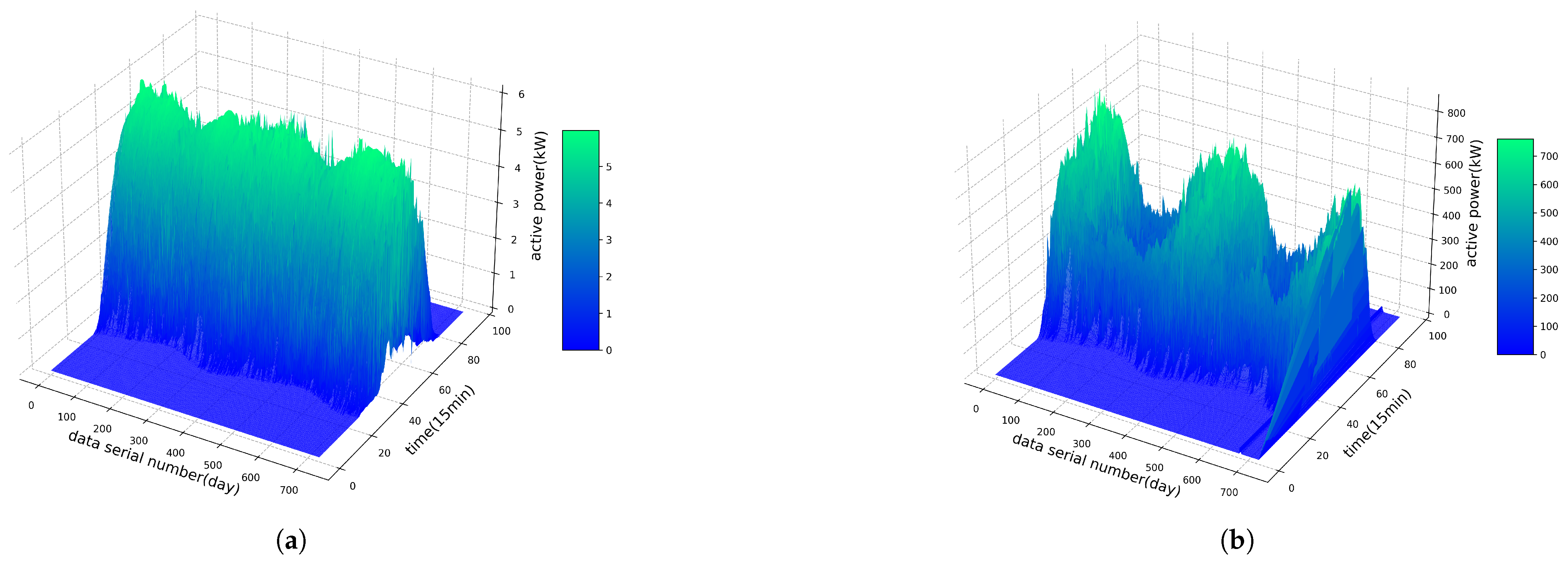
In this study, we conducted experimental analyses using two open-source PV power generation datasets from solar farms in Australia [34]. Dataset I was collected from the Alice Springs region and spans the period from 2015 to 2016, while Dataset II was obtained from the Desert Gardens area in Yulara, covering the period from 2017 to 2018. Both datasets were sampled at 15 min intervals, generating 96 data points per day. Dataset I contains 70,176 samples, and Dataset II has a comparable number of samples. Each sample records 13 key parameters, including timestamp, received active energy, active power, performance ratio, wind speed, ambient temperature, relative humidity, and other meteorological and power generation indicators. To evaluate the model performance, a time-ordered cross-validation approach was employed, with the final two months of each dataset reserved as an independent test set. Figure 5 illustrates the three-dimensional variations in PV power output over the two-year period. The results reveal a pronounced annual cycle, with higher power generation observed during the summer months and lower generation during the winter. Since the training set covers a complete annual cycle, it captures the seasonal characteristics of PV generation and effectively mitigates seasonal bias. Moreover, the last two months of data (corresponding to the Australian summer) exhibit generation patterns consistent with those of the previous year, thereby ensuring the representativeness of the test set and the fairness of the evaluation. Therefore, the data partitioning strategy adopted in this study meets the requirements of time-series forecasting tasks in terms of temporal continuity and consistency of data distribution.

To ensure data consistency, minimize the impact of outliers, prevent gradient vanishing, and enhance computational efficiency, data normalization is applied before prediction. The normalization process is defined as follows:

$$\begin{array}{c}\hfill x_{\mathrm{norm}}={\displaystyle \frac{x_i-min\left(x_i\right)}{max\left(x_i\right)-min\left(x_i\right)}}\end{array}$$

(20)

where $x_{norm}$ represents the normalized value; $x_i$ is the original input variable, $max\left(x_i\right)$ denotes the maximum value of the variable in the dataset, and $min\left(x_i\right)$ denotes the minimum value of the variable in the dataset. This normalization process maps all input values to the range [0, 1], preserving relative differences while eliminating scale dependencies.

5.2. Evaluation Metrics and Experimental Setup

To evaluate the prediction accuracy of the model, MSE, DTW, and TDI are employed as performance metrics. The corresponding mathematical formulations are as follows:

$$\begin{array}{c}\hfill \mathrm{MSE}={\displaystyle \frac{1}{N}}\sum _{i=1}^n{(y_i-x_i)}^2\end{array}$$

(21)

$$\begin{array}{c}\hfill {\mathrm{DTW}}_{\gamma }({\overline{y}}_i,y_i):=-\gamma log\left(\sum _{A\in A_{k,k}}exp\left(-{\displaystyle \frac{\langle A,\Delta ({\overline{y}}_i,y_i)\rangle }{\gamma }}\right)\right)\end{array}$$

(22)

$$\begin{array}{c}\hfill {\mathrm{TDI}}_{\gamma }({\overline{y}}_i,y_i):={\displaystyle \frac{1}{Z}}\sum _{A\in A_{k,k}}\langle A,\Omega \rangle exp\left(-{\displaystyle \frac{\langle A,\Delta ({\overline{y}}_i,y_i)\rangle }{\gamma }}\right)\end{array}$$

(23)

where $y_i$ represents the actual output value of the i-th data point in the test set, and $x_i$ denotes the predicted output value of the corresponding data point. N is the total number of samples in the test set. The detailed computational methods for DTW and TDI are provided in Section 3.3.

To assess the model’s effectiveness across different prediction horizons, the preprocessed dataset is structured into three distinct subsets. Each subset maintains a consistent input sequence length of 2880, while the corresponding label sequence lengths are set to 96, 192, and 288. The dataset is partitioned into training and testing sets following a 5:1 ratio, ensuring a balanced evaluation of the model’s generalization performance.

The experimental environment consists of an Intel i7-9700K processor and an NVIDIA GeForce RTX 3090 GPU (24 GB GDDR6X). The algorithmic model is implemented using Python 3.8, with the network architecture built on the open-source deep learning framework PyTorch. The Python libraries utilized in the experiments include pandas, numpy, matplotlib, torch, math, and time.

5.3. Prediction Performance of Different Models

This study evaluates the performance of classical Transformer models, the TCNformer designed for photovoltaic power forecasting, and the recent time-series model ConvTimeNet [35]. The Transformer-based baselines include Transformer, Reformer, Informer, and Autoformer. To ensure fair and reproducible forecasting, the datasets are split chronologically, reserving the final two months as the independent test set. A sliding window approach is applied to generate samples for 24 h (96 steps), 48 h (192 steps), and 72 h (288 steps) forecasting tasks. This method strictly preserves temporal order, prevents information leakage, and fully covers the test set, improving the representativeness and robustness of evaluations. All models use identical input and output lengths during training and testing to ensure a consistent and fair comparison. The forecasting results for different horizons are summarized in

Table 1. Prediction results of each model under different steps.

	24 h (96 Steps)			48 h (192 Steps)			72 h (288 Steps)
	MSE	DTW	TDI	MSE	DTW	TDI	MSE	DTW	TDI
Dataset I
Transformer	0.3638	1.3543	0.1887	0.6620	2.2196	0.3449	0.8908	2.7145	1.4573
Reformer	0.4007	1.3131	0.1016	0.4992	1.9624	0.1315	0.5849	2.5188	0.1256
Informer	0.3749	1.2574	0.3180	0.4879	2.1776	0.7757	0.5090	2.6955	0.5877
Autoformer	0.3674	1.4705	0.2147	0.4614	1.9709	0.3202	0.4630	2.3218	0.2781
TCNformer	0.1519	1.1385	0.3963	0.3285	1.5631	0.4214	0.5612	2.7412	0.5368
ConvTimeNet	0.1843	1.4115	0.2785	0.2445	2.0823	0.5237	0.3303	2.6724	0.6388
DTCformer	0.2872	1.2346	0.0537	0.2518	1.6660	0.2187	0.2961	2.1718	0.2342
Dataset II
Transformer	0.4352	1.6824	0.2287	0.7557	2.6265	0.3932	0.9221	2.9587	1.6165
Reformer	0.4558	1.5583	0.1288	0.5851	2.1983	0.1557	0.6756	2.8245	0.1489
Informer	0.4251	1.4235	0.3658	0.5512	2.3682	0.8793	0.5754	2.9108	0.7073
Autoformer	0.4117	1.7396	0.2562	0.5493	2.2650	0.3682	0.5278	2.6745	0.3152
TCNformer	0.1885	1.3150	0.4691	0.3698	1.7979	0.4810	0.6248	2.9687	0.5907
ConvTimeNet	0.1996	1.6142	0.3191	0.2716	2.1904	0.5894	0.3912	2.9769	0.7228
DTCformer	0.2937	1.4868	0.1097	0.2683	1.7708	0.2543	0.3453	2.3147	0.2664

.

Based on the experimental results, TCNformer demonstrates the lowest prediction error and highest accuracy among Transformer-based models in the 24 h forecasting scenario, despite exhibiting relatively higher temporal distortion as indicated by the TDI metric. The proposed DTCformer achieves the best TDI performance, and ranks second in DTW and third in MSE, following TCNformer and ConvTimeNet. These results further validate the superiority of TCNformer in short-term photovoltaic forecasting while highlighting the strong temporal alignment capability of DTCformer.

In the 48 h prediction scenario, the DTCformer model demonstrates one of the best MSE metrics, comparable to that of ConvTimeNet and showing a 23.34% improvement over the TCNformer model. Its DTW performance surpasses both the TCNformer and ConvTimeNet models, while its TDI metric is slightly lower than that of the Reformer model.

In the 72 h prediction scenario, the DTCformer model achieves the best performance in both the MSE and DTW metrics, although its TDI metric is slightly worse than that of the Reformer model. Notably, in both the 48 h and 72 h prediction scenarios, the Reformer model exhibits the best performance in the time loss metric, TDI. Further optimization of the DTCformer model could be derived from the Reformer network, aiming to explore predictive models with reduced time loss.

In summary, the DTCformer model exhibits strong performance in time-series forecasting tasks, particularly for long-term prediction, by integrating the temporal feature extraction capability of TCNformer with the long-range modeling strength of Autoformer. However, as shown in Table 1, DTCformer performs worse than ConvTimeNet and TCNformer in terms of MSE for short-term forecasts, and shows only marginal improvements across various metrics in mid- to long-term scenarios. This result can be largely attributed to the use of the DILATE loss, which jointly optimizes shape (DTW) and temporal (TDI) alignment. To further analyze this outcome, we calculated the DILATE values for all baseline models, as summarized in

Table 2. DILATE values of each model for different numbers of steps.

	24 h (96 Steps)	48 h (192 Steps)	72 h (288 Steps)
Dataset I
Transformer	0.7715	1.2822	2.0859
Reformer	0.7073	1.0469	1.3222
Informer	0.7877	1.4766	1.6416
Autoformer	0.8426	1.1456	1.2999
TCNformer	0.7674	0.9923	1.6390
ConvTimeNet	0.8450	1.3030	1.6556
DTCformer	0.6441	0.9424	1.2030
Dataset II
Transformer	0.9555	1.5098	2.2876
Reformer	0.8436	1.1770	1.4867
Informer	0.8946	1.6237	1.8091
Autoformer	0.9979	1.3167	1.4949
TCNformer	0.8921	1.1395	1.7797
ConvTimeNet	0.9667	1.3899	1.8499
DTCformer	0.7983	1.0126	1.2906

.

As shown in Table 2, for the DILATE metric, which accounts for both shape loss and time loss, the DTCformer model demonstrates the best performance in the 24 h, 48 h, and 72 h prediction scenarios.

5.4. Ablation Experiment

To evaluate the effectiveness of each optimized module in the DTCformer model, we conducted ablation experiments by removing each of the three innovative modules for comparison. Specifically, we established four experimental groups: the complete DTCformer model, the DTCformer model without the DILATE loss, the DTCformer model without the TCNForward module, and the DTCformer model without the Variable Selection Embedding module. In addition to evaluating the impact of removing each module individually, we further investigated the potential interaction effects by considering combinations of module removals. This comprehensive analysis allows us to assess not only the contribution of each component in isolation but also their synergistic influence on the overall model performance. The results of the ablation experiments are presented in

Table 3. Results of ablation experiments.

	24 h (96 Steps)			48 h (192 Steps)			72 h (288 Steps)
	MSE	DTW	TDI	MSE	DTW	TDI	MSE	DTW	TDI
DTCformer	0.2872	1.2346	0.0537	0.2518	1.6660	0.2187	0.2961	2.1718	0.2342
Without embed	0.3935	1.2487	0.2073	0.4564	1.8521	0.2227	0.5364	2.4761	0.2028
Without TCNForward	0.3100	1.3977	0.3116	0.3119	1.8822	0.2550	0.4478	2.7646	0.3490
Without DILATE	0.2925	1.4716	0.4048	0.2976	1.9232	0.3211	0.3369	2.4438	0.3123
Without embed + TCNForward	0.4210	1.5250	0.3892	0.4785	2.0031	0.3704	0.5722	2.9354	0.3895
Without embed + DILATE	0.4023	1.6189	0.4420	0.4628	2.0325	0.3915	0.5526	2.8153	0.3764
Without TCNForward + DILATE	0.3368	1.5943	0.4569	0.3483	2.0432	0.4082	0.4985	2.8946	0.4242

.

Based on the results presented in the table, the DTCformer model achieves optimal performance when all three key components—the VSE module, the TCNForward module, and the DILATE loss function—are integrated. Omitting the DILATE loss function results in prediction outcomes that closely resemble those of the complete DTCformer model in terms of the MSE metric; however, performance declines significantly in the DTW, TDI, and DILATE metrics. Similarly, excluding the Variable Selection Embedding module leads to a notable increase in MSE, indicating a considerable drop in predictive accuracy. Furthermore, when the TCNForward module is removed, the model exhibits a substantial increase in error, particularly in the 72 h prediction scenario. These findings highlight the importance of each component in enhancing the model’s predictive capability and robustness.

To further explore the potential interactions among key components, we conducted extended ablation studies by simultaneously removing two modules. The results demonstrate that jointly removing the VSE and TCNForward modules leads to the most severe performance degradation across all metrics, particularly for long-term forecasts, indicating their complementary roles in capturing feature relevance and temporal dependencies. Similarly, the simultaneous removal of the VSE module and the DILATE loss results in a marked decline in performance, especially in TDI, underscoring the combined benefits of effective feature selection and shape-aware optimization. Furthermore, the simultaneous removal of the TCNForward module and the DILATE loss causes significant deterioration in DTW and TDI, while moderately affecting MSE, suggesting their joint contribution to maintaining temporal coherence over extended forecasting horizons.

The experimental results confirm that the DTCformer architecture effectively achieves its design objectives through the synergistic integration of its key modules. The DILATE loss function extends beyond conventional MSE optimization by incorporating both temporal distortion and shape-aware metrics, facilitating a more comprehensive performance evaluation. The TCNForward module enhances temporal feature extraction via dilated causal convolutions, capturing both short-term and long-term dependencies with greater precision. Additionally, the VSE module employs adaptive feature weighting, improving predictive accuracy by effectively distinguishing and prioritizing relevant features. This modular design not only enables a more thorough understanding of temporal patterns but also maintains computational efficiency, reinforcing the model’s overall effectiveness.

5.5. Sensitivity Analysis

To assess the robustness and adaptability of the proposed model, we performed sensitivity analyses on two key factors using Dataset I: the trade-off coefficient $\alpha$ in the DILATE loss and the depth of the TCN architecture. The corresponding results are reported in

Table 4. Sensitivity analysis of the effect of the trade-off coefficient $\alpha$ on the DILATE value.

Trade-Off Coefficient $\mathit{\alpha }$	24 h (96 Steps)			48 h (192 Steps)			72 h (288 Steps)
	MSE	DTW	TDI	MSE	DTW	TDI	MSE	DTW	TDI
0.75	0.3810	1.1021	0.1443	0.3965	1.4402	0.2790	0.4508	1.8820	0.3101
0.5	0.2872	1.2346	0.0537	0.2518	1.6660	0.2187	0.2961	2.1718	0.2342
0.25	0.2726	1.3879	0.0341	0.2602	1.8027	0.1674	0.3193	2.3829	0.1910

and

Table 5. Sensitivity analysis of TCN depth.

TCN Depth (Layers)	24 h (96 Steps)			48 h (192 Steps)			72 h (288 Steps)
	MSE	DTW	TDI	MSE	DTW	TDI	MSE	DTW	TDI
1	0.3015	1.3041	0.0608	0.2669	1.7324	0.2360	0.3127	2.2456	0.2489
2	0.2872	1.2346	0.0537	0.2518	1.6660	0.2187	0.2961	2.1718	0.2342
3	0.2898	1.2453	0.0542	0.2457	1.5982	0.2023	0.2896	2.0665	0.2215

.

As shown in Table 4, smaller values of $\alpha$, which assign more weight to the TDI, generally improve the MSE and TDI, particularly for short-term horizons. However, an excessively low $\alpha$ (e.g., 0.25) slightly compromises DTW, especially in long-term predictions. In contrast, larger $\alpha$ values improve DTW by emphasizing shape alignment, but lead to notable increases in temporal errors. These results reveal a trade-off between shape fidelity and temporal precision inherent in the DILATE loss, and suggest that moderate $\alpha$ values (e.g., 0.5) offer a balanced performance across forecasting horizons.

Table 5 demonstrates that increasing the TCN depth from one to two layers significantly improves performance across all metrics. Further increasing it to three layers yields additional gains, especially for longer horizons, though marginal benefits diminish and short-term performance slightly fluctuates. A depth of two layers provides a good balance between model capacity and generalization.

These results highlight the importance of appropriately tuning both loss function parameters and model depth to ensure robust multi-horizon forecasting.

5.6. Computational Cost Analysis

All experiments were conducted using PyTorch 2.5.1 with CUDA 12.1. Dataset I was used with an input sequence length of 2880 steps, and prediction lengths of 96, 192, and 288 steps. All models were trained with a batch size of 16 and an early stopping strategy based on no improvement on the test set for 10 consecutive epochs. Computational efficiency was evaluated by training time per epoch (seconds) and inference throughput (samples per second).

Table 6. Comparison of DTCformer and baseline models on computational cost and inference speed.

Model	Training Time (s/epoch)			Throughput (samples/s)
	96 Steps	192 Steps	288 Steps	96 Steps	192 Steps	288 Steps
Transformer	120.3	152.31	185.17	48.28	35.41	27.64
Informer	41.32	47.80	52.45	110.12	102.36	90.15
Autoformer	48.25	63.93	68.55	105.25	98.38	85.27
TCNformer	55.16	56.46	61.28	117.56	110.73	92.21
ConvTimeNet	23.13	23.54	24.39	200.92	199.53	198.25
DTCformer	65.89	69.47	73.73	122.20	115.57	104.27

presents a comparison of training time per epoch and inference throughput between DTCformer and five baseline models. As expected, Transformer incurs the highest training cost and lowest inference throughput due to the quadratic complexity of its full-attention mechanism. DTCformer requires a moderately longer training time than Informer, Autoformer, and TCNformer, primarily due to the integration of the DILATE loss, which jointly optimizes temporal consistency and shape alignment. Despite being more computationally intensive than lightweight models like ConvTimeNet, DTCformer achieves substantially higher accuracy in long-term forecasting, justifying its complexity. In inference, it surpasses Transformer in efficiency and outperforms Informer, Autoformer, and TCNformer by 3.95% to 16.1% across all prediction lengths. These results demonstrate that DTCformer offers a well-balanced trade-off between computational cost and predictive performance, making it a promising solution for real-world PV forecasting, where both accuracy and efficiency are essential.

6. Conclusions

This study addresses the challenges of cumulative multi-step prediction errors in photovoltaic power forecasting and the limitations of traditional evaluation metrics (e.g., MSE, MAE) by proposing DTCformer, a generative forecasting model based on Autoformer. DTCformer integrates the TCNForward module, enabling hierarchical temporal feature extraction across multiple time scales. Additionally, it incorporates a VSE module, which utilizes a learnable embedding transformation mechanism to effectively capture inter-variable dependencies and temporal periodicity. This dual-pathway design enables the model to concurrently capture intra-variable temporal dynamics and inter-variable dependencies, thereby significantly enhancing the accuracy and robustness of photovoltaic power forecasting.

The experimental results demonstrate that DTCformer consistently delivers strong performance across multiple forecasting horizons, with particularly notable advantages in long-term prediction. It outperforms mainstream models such as Transformer, Informer, Autoformer, and ConvTimeNet in terms of DTW and TDI metrics. By incorporating the DILATE loss function, the model achieves joint optimization of shape fidelity and temporal alignment. Quantitatively, DTCformer improves DILATE performance by 8.9–23.6%, 5.0–36.2%, and 7.5–42.3% over baseline models in short-term (24 h), mid-term (48 h), and long-term (72 h) forecasting, respectively, with the most substantial improvement (42.3%) observed over Transformer in long-term forecasting. In terms of computational cost, although the integration of DILATE slightly increases training time, DTCformer achieves higher inference efficiency than all baseline models except the lightweight ConvTimeNet, with throughput improvements ranging from 3.95% to 16.1% over Informer, Autoformer, and TCNformer. Overall, DTCformer strikes a favorable balance between accuracy and efficiency, making it a promising solution for real-world photovoltaic forecasting applications.

Future research will focus on further optimizing the model architecture and exploring the broader applicability of DTCformer in diverse time-series forecasting tasks. In particular, photovoltaic forecasting under extreme conditions represents a key research direction, aimed at enhancing the model’s adaptability and generalization in complex real-world scenarios.

References

- Liu, B.; Song, C.; Wang, Q.; Wang, Y. Forecasting of China’s solar PV industry installed capacity and analyzing of employment effect: Based on GRA-BiLSTM model. Environ. Sci. Pollut. Res. 2022, 29, 4557–4573. [Google Scholar] [CrossRef] [PubMed]
- Zhu, Y.; Xu, X.; Yan, Z.; Lu, J. Data acquisition, power forecasting and coordinated dispatch of power systems with distributed PV power generation. Electr. J. 2022, 35, 107133. [Google Scholar] [CrossRef]
- Iweh, C.D.; Gyamfi, S.; Tanyi, E.; Effah-Donyina, E. Distributed generation and renewable energy integration into the grid: Prerequisites, push factors, practical options, issues and merits. Energies 2021, 14, 5375. [Google Scholar] [CrossRef]
- Massaoudi, M.; Chihi, I.; Abu-Rub, H.; Refaat, S.S.; Oueslati, F.S. Convergence of photovoltaic power forecasting and deep learning: State-of-art review. IEEE Access 2021, 9, 136593–136615. [Google Scholar] [CrossRef]
- Guermoui, M.; Bouchouicha, K.; Bailek, N.; Boland, J.W. Forecasting intra-hour variance of photovoltaic power using a new integrated model. Energy Convers. Manag. 2021, 245, 114569. [Google Scholar] [CrossRef]
- Vidal, A.; Kristjanpoller, W. Gold Volatility Prediction using a CNN-LSTM approach. Expert Syst. Appl. 2020, 157, 113481. [Google Scholar] [CrossRef]
- Shao, H.; Soong, B.H. Traffic flow prediction with long short-term memory networks (LSTMs). In Proceedings of the 2016 IEEE Region 10 Conference (TENCON), Singapore, 22–25 November 2016; pp. 2986–2989. [Google Scholar]
- Bae, S.H.; Choi, I.K.; Kim, N.S. Acoustic Scene Classification Using Parallel Combination of LSTM and CNN. DCASE 2016, 585, 11–15. [Google Scholar]
- Zhang, G.P. Time series forecasting using a hybrid ARIMA and neural network model. Neurocomputing 2003, 50, 159–175. [Google Scholar] [CrossRef]
- Dubey, A.K.; Kumar, A.; García-Díaz, V.; Sharma, A.K.; Kanhaiya, K. Study and analysis of SARIMA and LSTM in forecasting time series data. Sustain. Energy Technol. Assess. 2021, 47, 101474. [Google Scholar]
- Pai, P.F.; Lin, K.P.; Lin, C.S.; Chang, P.T. Time series forecasting by a seasonal support vector regression model. Expert Syst. Appl. 2010, 37, 4261–4265. [Google Scholar] [CrossRef]
- Zhou, H.; Zhang, S.; Peng, J.; Zhang, S.; Li, J.; Xiong, H.; Zhang, W. Informer: Beyond Efficient Transformer for Long Sequence Time-Series Forecasting. In Proc. AAAI Conf. Artif. Intell. 2021, 35, 11106–11115. [Google Scholar] [CrossRef]
- Lin, T.; Wang, Y.; Liu, X.; Qiu, X. A Survey of Transformers. AI Open 2022, 3, 111–132. [Google Scholar] [CrossRef]
- Wu, H.; Xu, J.; Wang, J.; Long, M. Autoformer: Decomposition Transformers with Auto-Correlation for Long-Term Series Forecasting. Adv. Neural Inf. Process. Syst. 2021, 34, 22419–22430. [Google Scholar]
- Kitaev, N.; Kaiser, Ł.; Levskaya, A. Reformer: The Efficient Transformer. arXiv 2020, arXiv:2001.04451. [Google Scholar]
- Mellit, A.; Massi Pavan, A.; Ogliari, E.; Leva, S.; Lughi, V. Advanced methods for photovoltaic output power forecasting: A review. Appl. Sci. 2020, 10, 487. [Google Scholar] [CrossRef]
- Larson, D.P.; Nonnenmacher, L.; Coimbra, C.F. Day-Ahead Forecasting of Solar Power Output from Photovoltaic Plants in the American Southwest. Renew. Energy 2016, 91, 11–20. [Google Scholar] [CrossRef]
- Dhimish, M.; Lazaridis, P.I. Approximating shading ratio using the total-sky imaging system: An application for photovoltaic systems. Energies 2022, 15, 8201. [Google Scholar] [CrossRef]
- Jang, H.S.; Bae, K.Y.; Park, H.S.; Sung, D.K. Solar Power Prediction Based on Satellite Images and Support Vector Machine. IEEE Trans. Sustain. Energy 2016, 7, 1255–1263. [Google Scholar] [CrossRef]
- Benmouiza, K.; Cheknane, A. Small-Scale Solar Radiation Forecasting Using ARMA and Nonlinear Autoregressive Neural Network Models. Theor. Appl. Climatol. 2016, 124, 945–958. [Google Scholar] [CrossRef]
- Mahalingam, A.; Thatte, S.; Narkhede, Y.; Brid, Y.; Mane, D. A Survey of Photovoltaic Power Forecasting Approaches in Solar Energy Landscape. In Computational Methods in Science and Technology; CRC Press: Boca Raton, FL, USA, 2024; pp. 87–101. [Google Scholar]
- De Leone, R.; Pietrini, M.; Giovannelli, A. Photovoltaic Energy Production Forecast Using Support Vector Regression. Neural Comput. Appl. 2015, 26, 1955–1962. [Google Scholar] [CrossRef]
- Yakowitz, S. Nearest-Neighbour Methods for Time Series Analysis. J. Time Ser. Anal. 1987, 8, 235–247. [Google Scholar] [CrossRef]
- Zagouras, A.; Pedro, H.T.; Coimbra, C.F. On the Role of Lagged Exogenous Variables and Spatio–Temporal Correlations in Improving the Accuracy of Solar Forecasting Methods. Renew. Energy 2015, 78, 203–218. [Google Scholar] [CrossRef]
- Yu, Y.; Cao, J.; Zhu, J. An LSTM short-term solar irradiance forecasting under complicated weather conditions. IEEE Access 2019, 7, 145651–145666. [Google Scholar] [CrossRef]
- Sethi, R.; Kleissl, J. Comparison of short-term load forecasting techniques. In Proceedings of the 2020 IEEE Conference on Technologies for Sustainability (SusTech), Santa Ana, CA, USA, 23–25 April 2020; pp. 1–6. [Google Scholar]
- Alzahrani, A.; Shamsi, P.; Ferdowsi, M.; Dagli, C. Solar irradiance forecasting using deep recurrent neural networks. In Proceedings of the 2017 IEEE 6th International Conference on Renewable Energy Research and Applications (ICRERA), San Diego, CA, USA, 5–8 November 2017; pp. 988–994. [Google Scholar]
- Wang, F.; Zhen, Z.; Liu, C.; Mi, Z.; Hodge, B.M.; Shafie-khah, M.; Catalão, J.P. Image phase shift invariance based cloud motion displacement vector calculation method for ultra-short-term solar PV power forecasting. Energy Convers. Manag. 2018, 157, 123–135. [Google Scholar] [CrossRef]
- Wojtkiewicz, J.; Hosseini, M.; Gottumukkala, R.; Chambers, T.L. Hour-ahead solar irradiance forecasting using multivariate gated recurrent units. Energies 2019, 12, 4055. [Google Scholar] [CrossRef]
- Gao, B.; Huang, X.; Shi, J.; Tai, Y.; Zhang, J. Hourly forecasting of solar irradiance based on CEEMDAN and multi-strategy CNN-LSTM neural networks. Renew. Energy 2020, 162, 1665–1683. [Google Scholar] [CrossRef]
- West, M. Time series decomposition. Biometrika 1997, 84, 489–494. [Google Scholar] [CrossRef]
- Le Guen, V.; Thome, N. Shape and time distortion loss for training deep time series forecasting models. In Proceedings of the 32nd International Conference on Neural Information Processing Systems (NeurIPS), Vancouver, BC, Canada, 8–14 December 2019; pp. 15963–15973. [Google Scholar]
- Rangapuram, S.S.; Seeger, M.W.; Gasthaus, J.; Stella, L.; Wang, Y.; Januschowski, T. Deep state space models for time series forecasting. In Proceedings of the 31st International Conference on Neural Information Processing Systems (NeurIPS), Montréal, QC, Canada, 3–8 December 2018; pp. 7785–7794. [Google Scholar]
- Desert Knowledge Australia Centre. Download Data: Yulara Solar System. Available online: http://dkasolarcentre.com.au/historical-data/download (accessed on 15 November 2023).
- Cheng, M.; Yang, J.; Pan, T.; Liu, Q.; Li, Z. Convtimenet: A Deep Hierarchical Fully Convolutional Model for Multivariate Time Series Analysis. arXiv 2024, arXiv:2403.01493. [Google Scholar]