Leveraging Harris Hawks Optimization for Enhanced Multi-Objective Optimal Power Flow in Complex Power Systems

Abstract

The utilization of Harris Hawks Optimization (HHO) for Multi-Objective Optimal Power Flow (MaO-OPF) challenges presented in this paper is both novel and compelling, as this approach has not been previously applied to these types of optimization problems. HHO, which shares characteristics with ant behavior, demonstrates significant strength in addressing high-dimensional, nonlinear optimization issues within power systems. In this study, HHO is implemented on an IEEE 30-bus power system, optimizing six competing objectives: minimizing total fuel cost, emissions, active power loss, reactive power loss, reducing voltage deviation, and enhancing voltage steady state. The effectiveness of HHO is assessed by comparing its performance to two alternative methods, MOEA/D-DRA and NSGA-III. Experimental results reveal that solutions derived from HHO exhibit superior convergence, enhanced diversity maintenance, and higher quality Pareto-optimal solutions compared to the MOEA/D trail algorithms. The research breaks new ground in the application of the Harris Hawks Optimization (HHO) algorithm to the Multi-Objective Optimal Power Flow (MaO-OPF) problem. The restructuring not only incorporates self-adaptive constraint-handling techniques and dynamic exploration exploitation strategies, but also addresses the more pressing requirements of modern power systems with even better convergence, and both sequential and global computational efficiency than existing skill. This approach proves to be a powerful and effective solution for addressing the complex challenges associated with MaO, enabling power systems to manage multiple conflicting objectives more efficiently.

1. Introduction

The Multi-Objective Optimal Power Flow (MaO-OPF) problem has become increasingly complex due to the ongoing expansion of modern electrical power networks and the rising integration of various renewable energy sources [1,2]. This complexity surpasses that of previous models, as optimization focused solely on a single power flow objective is no longer sufficient. The challenge now includes balancing trade-offs among emissions, levels of active and reactive power losses, voltage stability, system reliability, and fuel costs, among other factors. Addressing the MaO-OPF problem is essential for the development of sustainable, cost-effective, and reliable energy systems.

1.1. Background and Impetus for the Study

Optimal Power Flow (OPF) has been a fundamental concern in power systems since Carpenter’s pioneering work in 1962, which framed OPF as an optimization problem involving cost and operational considerations under various constraints [3,4,5]. Traditional methods, such as Newton’s method [6], linear programming [7], and interior-point methods [8], have successfully addressed single-objective, low-dimensional problems. However, these conventional techniques have become inadequate in the context of modern power networks, which are more complex and geographically expansive. Recent advancements have highlighted the limitations of approaches that optimize a single response function, indicating that balancing cost, stability, and operational efficiency now necessitates multi-objective optimization techniques [9,10]. Consequently, meta-heuristic methods have gained prominence among researchers due to their adaptability, lower computational requirements, and effectiveness in solving high-dimensional, non-convex problems [11,12,13,14]. Recent advancements in meta-heuristic optimization techniques, such as those discussed in [15,16,17,18,19], have demonstrated substantial improvements in addressing the high-dimensional, nonlinear, and multi-objective optimization problems encountered in modern power systems.

1.2. Related Works and Limitations

A novel perspective was introduced by Rao et al. [20] through the Teaching-Learning-Based Optimization (TLBO), which incorporates a teacher-learner model to enhance search diversity and convergence. The modified version, MaOTLBO, integrates a reference point mechanism aimed at optimizing the MaO-OPF problem efficiently. However, comparisons of convergence towards the Pareto front in multi-objective OPF formulations remain crucial, as these algorithms are often computationally intensive and sensitive to parameter settings [21]. Jangir et al. (2018) [22] also applied MaOTLBO in power systems, yet it was outperformed by MOEA/D-DRA and NSGA-III, which provided more robust, well-distributed solutions to diverse objectives. While the multi-objective TLBO and the original TLBO algorithm have significantly advanced the field, they still suffer from slow convergence and instability in complex power systems characterized by oscillatory loads and stringent constraints. In recent advancements, Pareto-based methods such as the one proposed in ‘A new many-objective evolutionary algorithm based on generalized Pareto dominance’ (IEEE Transactions on Cybernetics, 2022) [23] have demonstrated superior performance in handling high-dimensional optimization tasks. This study incorporates this method as an additional benchmark to ensure a comprehensive evaluation of the proposed MaOHHO algorithm.

1.3. Research Gaps and Proposed Contributions

Despite the advancements in optimizing TLBO and evolutionary algorithms, there remains a substantial gap in techniques specifically addressing the MaO-OPF problem, which requires a seamless balance between exploration and exploitation across multiple objectives. These algorithms, particularly classical MOEAs and TLBO-based methods, struggle to maintain competitiveness and a diverse solution set as dimensionality increases due to conflicting objectives. Additionally, challenges such as parameter sensitivity and NP-completeness present significant obstacles in solving real-world MaO-OPF issues.

This study aims to address these gaps through the implementation of Harris Hawks Optimization (HHO), an algorithm inspired by the cooperative hunting behavior of Harris hawks, which incorporates both exploration and exploitation phases. Developed by Heidari et al. (2019) [24], HHO has emerged as a promising method for high-dimensional, non-convex optimization tasks, utilizing weight and dimensional factors that simulate the adaptive predatory behavior of Harris hawks. Given its evolving search mechanism, HHO appears well-suited for MaO-OPF problems, as it can conduct a thorough search without becoming trapped in local optima.

This paper proposes several key contributions to solving the MaO-OPF problem.

• Use of HHO to MaO-OPF: This is the first known case where HHO is used to address the multiobjective characteristics of power flow optimization problems.
• Adaptive Constraint-Handling Mechanisms: A unified penalty-repair function method guarantees feasibility even in the case of tight operating constraints.
• Dynamic Exploration-Exploitation Balance: The algorithm also uses Hawk’s hunting strategies which are effective in modifying the search behavior of the algorithm to avoid stagnation and improve solution quality.
• Efficient Pareto-Optimal Solution Generation: The use of the new method improves convergence and diversity metrics much more than state of art algorithms such as NSGA-III and MOEA/D-DRA—by making parameter-free optimization and historical data the primary approach.

1.4. Integration of HHO with OPF Problem

The Harris Hawks Optimization (HHO) algorithm has undergone steady evolution and possesses unique optimization techniques that enable it to address issues in the Optimal Power Flow (OPF) problem. The algorithm’s origin stems from the natural strategy used by Harris hawks during hunting. It employs a combination of exploration and exploitation phases, making it useful and expedient in solving highly dimensional and nonlinear problems.

The key reasons for selecting HHO for OPF include:

• Dynamic Exploration-Exploitation Balance: HHO incorporates automatic features that make it effective in evading local minima which is a challenge in OPF containing conflicting objectives.
• Constraint-Handling Capability: This enables the algorithm to combine penalty and recovery approaches to adhere to tight operating limits in a power system.
• Computational Efficiency: HHO features superior convergence rate than regular met heuristics hence being suitable for real time dealings in power systems.
• Pareto-Optimal Solutions: HHO employs adaptive pounced strategies along with a saturate babbling population which ensures that a great number of sparsely populated Pareto optimal solutions are created which are important for multi-objective OPF problems.

1.5. Paper Organization

This paper is structured as follows: Section 2 offers a comprehensive overview of the MaO-OPF problem, detailing its objectives, constraints, and mathematical formulations. Section 3 introduces the Hybrid Harmony Search algorithms, including modifications tailored for the MaO-OPF context. Section 4 presents an empirical study that evaluates and compares the performance of HHO on the IEEE 30-bus system. Finally, Section 5 concludes the paper by summarizing the contributions made and proposing avenues for future research regarding the application of HHO in power system optimization.

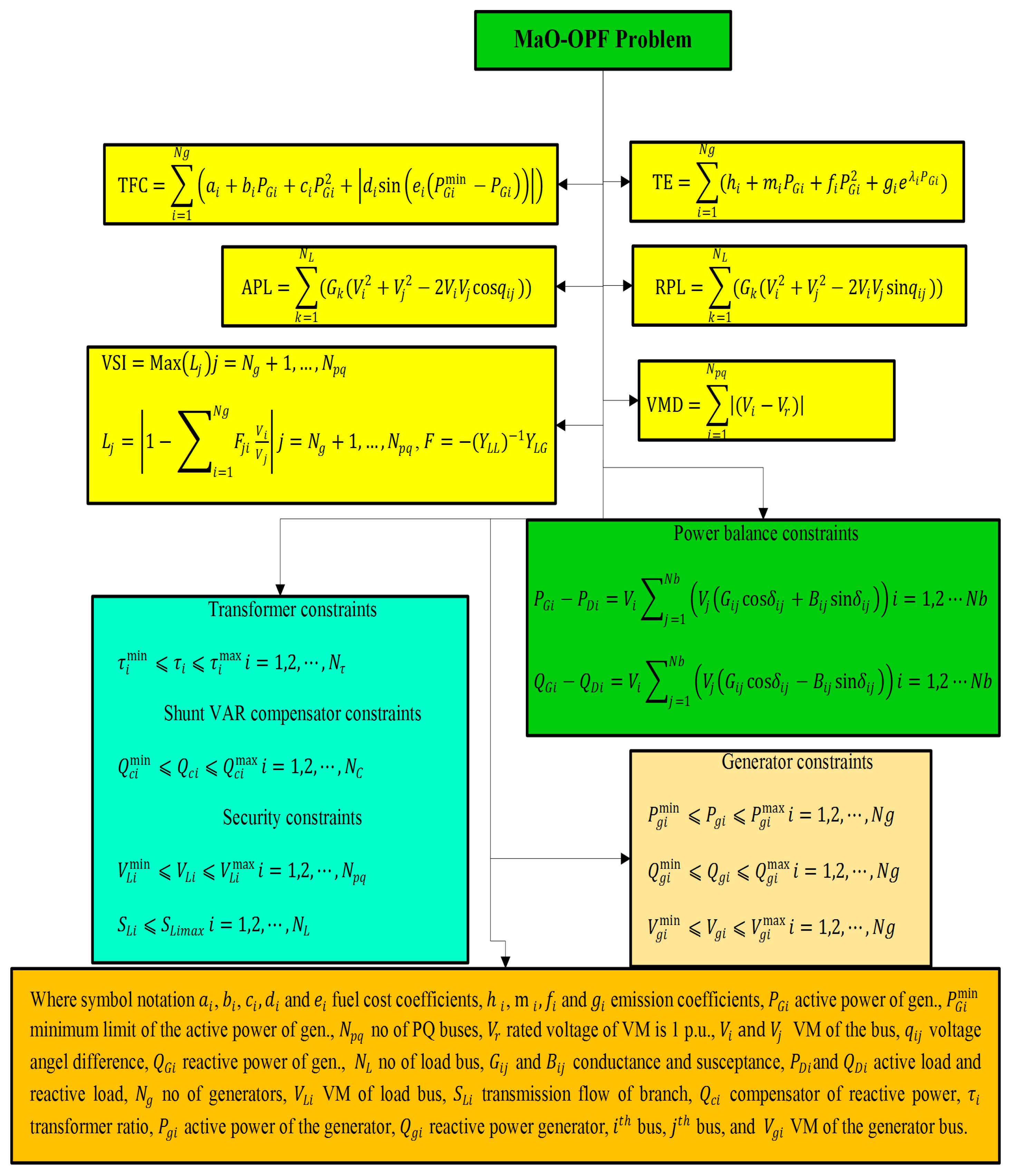
2. Multi-Objective Optimal Power Flow (MaO-OPF) Problem Formulation

The challenges inherent in the multi-objective OPF problem revolve around the optimization of various requirements within a power system. The primary focus of this multi-objective dimensional analysis is outlined as follows:

$$\begin{array}{c}\mathrm{M}\mathrm{i}\mathrm{n}\mathrm{i}\mathrm{m}\mathrm{i}\mathrm{z}\mathrm{e}\left[{\mathrm{g}}_1\left(\mathrm{v}\right){\mathrm{g}}_2\left(\mathrm{v}\right)\cdots {\mathrm{g}}_{\mathrm{L}}\left(\mathrm{v}\right)\right]\\ \mathrm{W}\mathrm{h}\mathrm{i}\mathrm{l}\mathrm{e} \mathrm{c}\mathrm{o}\mathrm{n}\mathrm{s}\mathrm{i}\mathrm{d}\mathrm{e}\mathrm{r}\mathrm{i}\mathrm{n}\mathrm{g:}\\ \left\{\begin{array}{c}{\mathrm{t}}_{\mathrm{j}}\left(\mathrm{v}\right)=0, \mathrm{v}=\mathrm{1,2},\cdots ,\mathrm{M}\\ {\mathrm{u}}_{\mathrm{i}}\left(\mathrm{v}\right)⩾0, \mathrm{i}=\mathrm{1,2},\cdots ,\mathrm{N}\mathrm{}\end{array}\right.\end{array}$$

(1)

In this context, M and N denote the number of inequalities and equalities included in the formulation, respectively. Meanwhile, L refers to the number of objectives, or more commonly, cost functions, which typically exceeds three in multi-objective optimization scenarios. Furthermore, g is the objective function; t and u represent the constraints functions.

2.1. Problem Overview

In electric power systems, the MaO-OPF problem aims to identify the optimal configuration of control variables that satisfy various system-specific objectives and associated constraints [25,26]. The goals encompassed within the MaO-OPF formulation include fuel consumption, carbon emissions, active and reactive power losses, voltage deviations, and indicators of voltage stability. These objectives are influenced by the dynamic nature and resilience requirements of modern power networks (see Figure 1). Ultimately, the MaO-OPF problem is critical for the efficient and effective operation of the power system, as each objective directly affects system performance, operational costs, and overall emissions.

2.2. Objectives

The following six objectives are commonly considered in MaO-OPF for power systems:

• Minimization of Fuel Cost (TFC):

The minimization of fuel cost can be summarized in relation (2):

$$\mathrm{TFC}={\sum }_{\mathrm{i}=1}^{{\mathrm{N}}_{\mathrm{G}}}({\mathrm{a}}_{\mathrm{i}}{{\mathrm{P}}_{\mathrm{G},\mathrm{i}}}^2+{\mathrm{b}}_{\mathrm{i}}{\mathrm{P}}_{\mathrm{G},\mathrm{i}}+{\mathrm{c}}_{\mathrm{i}})$$

(2)

where ${\mathrm{P}}_{\mathrm{G},\mathrm{i}}$ is the power generated by generator i, and ${\mathrm{a}}_{\mathrm{i}}$, ${\mathrm{b}}_{\mathrm{i}}$, and ${\mathrm{c}}_{\mathrm{i}}$ are cost coefficients for each generator.

2.

Minimization of Emission (TE):

The minimization of emissions is depicted as in relation (3):

$$\mathrm{TE}={\sum }_{\mathrm{i}=1}^{{\mathrm{N}}_{\mathrm{G}}}({\mathsf{\alpha }}_{\mathrm{i}}{{\mathrm{P}}_{\mathrm{G},\mathrm{i}}}^2+{\mathsf{\beta }}_{\mathrm{i}}{\mathrm{P}}_{\mathrm{G},\mathrm{i}}+{\mathsf{\gamma }}_{\mathrm{i}}+{\mathsf{\eta }}_{\mathrm{i}}\mathrm{e}\mathrm{x}\mathrm{p}({\mathsf{\delta }}_{\mathrm{i}}{\mathrm{P}}_{\mathrm{G},\mathrm{i}}\left)\right)$$

(3)

where ${\mathsf{\alpha }}_{\mathrm{i}}$, ${\mathsf{\beta }}_{\mathrm{i}}$, ${\mathsf{\gamma }}_{\mathrm{i}}$, ${\mathsf{\eta }}_{\mathrm{i}}$, and ${\mathsf{\delta }}_{\mathrm{i}}$ are emission coefficients for each generator.

3.

Minimization of Active Power Loss (APL):

The minimization of the active power loss is presented as in Equation (4):

$$\mathrm{APL}={\sum }_{\mathrm{i}=1}^{{\mathrm{N}}_{\mathrm{L}}}({\mathrm{G}}_{\mathrm{i}}{{\mathrm{V}}_{\mathrm{i}}}^2-2{\mathrm{V}}_{\mathrm{i}}{\mathrm{V}}_{\mathrm{j}}{\mathrm{G}}_{\mathrm{i}\mathrm{j}}\cos {\mathsf{\theta }}_{\mathrm{i}\mathrm{j}})$$

(4)

where ${\mathrm{G}}_{\mathrm{i}}$ and ${\mathrm{G}}_{\mathrm{i}\mathrm{j}}$ are conductance terms, ${\mathrm{V}}_{\mathrm{i}}$ and ${\mathrm{V}}_{\mathrm{j}}$ are bus voltages, and ${\mathsf{\theta }}_{\mathrm{i},\mathrm{j}}$ is the phase angle difference between buses i and j.

4.

Minimization of Reactive Power Loss (RPL):

The minimization of the reactive power loss is presented as in Equation (5):

$$\mathrm{RPL}={\sum }_{\mathrm{i}=1}^{{\mathrm{N}}_{\mathrm{L}}}({\mathrm{B}}_{\mathrm{i}}{{\mathrm{V}}_{\mathrm{i}}}^2-2{\mathrm{V}}_{\mathrm{i}}{\mathrm{V}}_{\mathrm{j}}{\mathrm{B}}_{\mathrm{i}\mathrm{j}}\sin {\mathsf{\theta }}_{\mathrm{i}\mathrm{j}})$$

(5)

where ${\mathrm{B}}_{\mathrm{i}}$ and ${\mathrm{B}}_{\mathrm{i}\mathrm{j}}$ are susceptance terms.

5.

Minimization of Voltage Magnitude Deviation (VMD):

The relation characterizing the minimization of the voltage magnitude deviation is presented in Equation (6):

$$\mathrm{VMD}={\sum }_{\mathrm{i}=1}^{{\mathrm{N}}_{\mathrm{B}}}|{\mathrm{V}}_{\mathrm{i}}-\mathrm{}{\mathrm{V}}_{\mathrm{r}\mathrm{e}\mathrm{f}}|$$

(6)

where ${\mathrm{V}}_{\mathrm{i}}$ is the voltage at bus i and ${\mathrm{V}}_{\mathrm{r}\mathrm{e}\mathrm{f}}$ is the reference voltage.

6.

Maximization of Voltage Stability Index (VSI): A stability index, such as the Line Stability Index (L-index), can be used for VSI as described in relation (7):

$$\mathrm{VSI}=1-({\displaystyle \frac{1}{{\mathrm{V}}_{\mathrm{i}}}}{\sum }_{\mathrm{j}=1}^{\mathrm{N}}{\mathrm{V}}_{\mathrm{j}}{\mathrm{Y}}_{\mathrm{i}\mathrm{j}}\mathrm{\angle }{\mathsf{\theta }}_{\mathrm{i}\mathrm{j}})$$

(7)

where ${\mathrm{Y}}_{\mathrm{i}\mathrm{j}}$ represents admittance values between buses.

The VSI parameter is defined mathematically, through the very important L-index, as stated in Equation (7). The voltage stability index (VSI) measures closeness to voltage collapse, with its values tending towards 1 being less stable and those tending towards 0 being more stable. The scenario of voltage instability is a very serious threat to modern power systems as it often results in power outages and economic downturn. In case power systems with high penetration of renewable sources are considered, they usually experience rapid fluctuations in load and generation; hence robust optimization of the VSI Criterion becomes a focus of the MaO-OPF problem. In practical scenarios however, MaO-OPF ensures a consistently high value of Voltage stability index; this in turn serves as a check against approaches or techniques that tend to cause the voltage to hit its collapse point through the system’s operating limits. Hence the inclusion of VSI as an objective in OPF framework design enhances operational security of the practical electricity network.

2.3. Constraints

MaO-OPF must satisfy both equality and inequality constraints to ensure safe, reliable, and stable power system operation:

• Equality Constraints:

  ○

  Power Balance Equations:

$${\mathrm{P}}_{\mathrm{G},\mathrm{i}}-{\mathrm{P}}_{\mathrm{D},\mathrm{i}}={\mathrm{V}}_{\mathrm{i}}{\sum }_{\mathrm{j}=1}^{\mathrm{N}}{\mathrm{V}}_{\mathrm{j}}\left({\mathrm{G}}_{\mathrm{i}\mathrm{j}}\cos {\mathsf{\theta }}_{\mathrm{i}\mathrm{j}}+{\mathrm{B}}_{\mathrm{i}\mathrm{j}}\cos {\mathsf{\theta }}_{\mathrm{i}\mathrm{j}}\right)$$

(8)

$${\mathrm{Q}}_{\mathrm{G},\mathrm{i}}-{\mathrm{Q}}_{\mathrm{D},\mathrm{i}}={\mathrm{V}}_{\mathrm{i}}{\sum }_{\mathrm{j}=1}^{\mathrm{N}}{\mathrm{V}}_{\mathrm{j}}\left({\mathrm{G}}_{\mathrm{i}\mathrm{j}}\sin {\mathsf{\theta }}_{\mathrm{i}\mathrm{j}}-{\mathrm{B}}_{\mathrm{i}\mathrm{j}}\sin {\mathsf{\theta }}_{\mathrm{i}\mathrm{j}}\right)$$

(9)

where ${\mathrm{P}}_{\mathrm{D},\mathrm{i}}$ and ${\mathrm{Q}}_{\mathrm{D},\mathrm{i}}$ are the active and reactive power demands at bus i.

2.

Inequality Constraints:

○

Generator Constraints:

$${{\mathrm{P}}_{\mathrm{G},\mathrm{i}}}^{\mathrm{m}\mathrm{i}\mathrm{n}}\le {\mathrm{P}}_{\mathrm{G},\mathrm{i}}\le {{\mathrm{P}}_{\mathrm{G},\mathrm{i}}}^{\mathrm{m}\mathrm{a}\mathrm{x}}$$

(10)

$${{\mathrm{Q}}_{\mathrm{G},\mathrm{i}}}^{\mathrm{m}\mathrm{i}\mathrm{n}}\le {\mathrm{Q}}_{\mathrm{G},\mathrm{i}}\le {{\mathrm{Q}}_{\mathrm{G},\mathrm{i}}}^{\mathrm{m}\mathrm{a}\mathrm{x}}$$

(11)

○

Voltage Constraints:

$${{\mathrm{V}}_{\mathrm{i}}}^{\mathrm{m}\mathrm{i}\mathrm{n}}\le {\mathrm{V}}_{\mathrm{i}}\le {{\mathrm{V}}_{\mathrm{i}}}^{\mathrm{m}\mathrm{a}\mathrm{x}}$$

(12)

○

Transformer Tap Settings and Shunt Capacitors: Defined to maintain voltage stability and to minimize losses.

The

Table 1. Objective Functions and Constraint Violations in MaO-OPF.

Objective	Expression	Penalty Factor
Total Fuel Cost (TFC)	TFC = $\sum _{\mathrm{i}=1}^{{\mathrm{N}}_{\mathrm{G}}}({\mathrm{a}}_{\mathrm{i}}{{\mathrm{P}}_{\mathrm{G},\mathrm{i}}}^2+{\mathrm{b}}_{\mathrm{i}}{\mathrm{P}}_{\mathrm{G},\mathrm{i}}+{\mathrm{c}}_{\mathrm{i}})$	10
Total Emission (TE)	$\mathrm{TE}=\sum _{\mathrm{i}=1}^{{\mathrm{N}}_{\mathrm{G}}}({\mathsf{\alpha }}_{\mathrm{i}}{{\mathrm{P}}_{\mathrm{G},\mathrm{i}}}^2+{\mathsf{\beta }}_{\mathrm{i}}{\mathrm{P}}_{\mathrm{G},\mathrm{i}}+{\mathsf{\gamma }}_{\mathrm{i}}+{\mathsf{\eta }}_{\mathrm{i}}\mathrm{e}\mathrm{x}\mathrm{p}({\mathsf{\delta }}_{\mathrm{i}}{\mathrm{P}}_{\mathrm{G},\mathrm{i}}\left)\right)$	20
Voltage Stability Index (VSI) / Voltage Magnitude Deviation (VMD)	$\mathrm{VSI}=1-({\displaystyle \frac{1}{{\mathrm{V}}_{\mathrm{i}}}}\sum _{\mathrm{j}=1}^{\mathrm{N}}{\mathrm{V}}_{\mathrm{j}}{\mathrm{Y}}_{\mathrm{i}\mathrm{j}}\mathrm{\angle }{\mathsf{\theta }}_{\mathrm{i}\mathrm{j}})$ VMD = $\sum _{\mathrm{i}=1}^{{\mathrm{N}}_{\mathrm{B}}}|{\mathrm{V}}_{\mathrm{i}}-{\mathrm{V}}_{\mathrm{r}\mathrm{e}\mathrm{f}}|$	15
Active Power Loss (APL) / Reactive Power Loss (RPL)	APL = $\sum _{\mathrm{i}=1}^{{\mathrm{N}}_{\mathrm{L}}}({\mathrm{G}}_{\mathrm{i}}{{\mathrm{V}}_{\mathrm{i}}}^2-2{\mathrm{V}}_{\mathrm{i}}{\mathrm{V}}_{\mathrm{j}}{\mathrm{G}}_{\mathrm{i}\mathrm{j}}\cos {\mathsf{\theta }}_{\mathrm{i}\mathrm{j}})$ RPL = $\sum _{\mathrm{i}=1}^{{\mathrm{N}}_{\mathrm{L}}}({\mathrm{B}}_{\mathrm{i}}{{\mathrm{V}}_{\mathrm{i}}}^2-2{\mathrm{V}}_{\mathrm{i}}{\mathrm{V}}_{\mathrm{j}}{\mathrm{B}}_{\mathrm{i}\mathrm{j}}\sin {\mathsf{\theta }}_{\mathrm{i}\mathrm{j}})$	12

presents objective functions, their expressions, as well as penalties for violating constraints.

2.4. Key Variables and Parameters

Table 2. Summary of Symbols and Parameters in Section 2.

Symbol	Description	Units
${\mathrm{P}}_{\mathrm{G},\mathrm{i}}$	Power generated by generator i	MW
ai,bi,ci	Cost coefficients for generator i	Currency/MW, etc.
αi, βi, γi, δi, ζi,	Emission coefficients for generator i	-
${\mathrm{G}}_{\mathrm{i}\mathrm{j}}$	Conductance between buses i and j	Siemens (S)
${\mathrm{B}}_{\mathrm{i}\mathrm{j}}$	Susceptance between buses i and j	Siemens (S)
${\mathrm{V}}_{\mathrm{i}}$	Voltage magnitude at bus i	p.u.
Vref	Reference voltage magnitude	p.u.
θij	Phase angle difference between buses i and j	Radians
ΔVi	Voltage deviation at bus i	p.u.
Lij	Line stability index between buses i and j	-
E	Total system emissions	kg/h
C	Total system cost	Currency/h
Λ	Penalty factor for cost-related constraint violations	-
μ	Penalty factor for emission-related constraint violations	-
fobj	Objective function for optimization (fuel cost, emissions, etc.)	-
Pd,i	Active power demand at bus i	MW
Qd,i	Reactive power demand at bus i	MVAr
Pl	Total active power loss	MW
Ql	Total reactive power loss	MVAr
Qc	Reactive power supplied by shunt capacitor banks	MVAr
T	Transformer tap setting	p.u.
ϵ	Constraint violation threshold	-

below is a proposed table of symbols used above. This table summarizes the key variables and parameters used in those equations:

3. Harris Hawks Optimization Algorithm for MaO-OPF

3.1. Overview of Harris Hawks Optimization (HHO)

3.1.1. History

Louis Lefebvre first established the link between birds and intelligence in 1997, drawing from his analysis of their distinct foraging behaviors. According to his research, hawks are recognized as some of the most intelligent bird species [27,28,29,30]. Among these is the Harris’s hawk (Parabuteo unicinctus), which is prevalent in Southern Arizona, USA, along with several other significant raptor species [31]. Unlike most carnivorous mammals that engage in solitary foraging, which involves individuals searching for food and sharing their findings, the social structure of the Harris’s hawk facilitates cooperative foraging among family members. This species is particularly noted for its exceptional hunting skills, especially in targeting other raptors. Bednarz conducted a meticulous study of this behavior pattern in his 1998 research on raptors [32].

Harris’s hawks typically travel in flocks, taking flight from tall trees or telephone poles at dawn, exhibiting a high level of skill and mutual trust. After executing a series of rapid flights, they regroup at elevated perches. Their primary strategy for locating concealed prey, such as rabbits, involves a unique collaborative movement technique known as “leapfrogging”, where they alternate between coming together and spreading out to enhance their coverage area.

One notable tactic employed by Harris’s hawks is the “pounce-and-surprise” technique, also referred to as “seven kills”. In this strategy, a group of hawks simultaneously descends on a single hidden rabbit from multiple directions, allowing for rapid capture. They adapt various chasing techniques depending on the circumstances and the nature of their prey. If the lead hawk loses sight of the prey during the descent, other hunters are ready to take over the pursuit. This role-switching strategy significantly increases the likelihood of successfully exhausting the fleeing rabbit. Once the most experienced and resilient hawk captures the weary prey, it brings it back to the group for sharing, effectively preventing the rabbit from escaping and using its evasive abilities to outmaneuver the others. Figure 2 illustrates some of the key behavioral traits of the Harris’s hawk in its natural habitat.

Furthermore, the hunting tactics of the Harris’s hawk demonstrate that the exploration and exploitation phases of the HHO algorithm are distinctly structured. These hawks employ advanced pounce techniques along with various other attack forms. In contrast to the normalized blood injury treatment algorithm, the HHO approach offers a stepwise method for enhancing a population’s performance, making it applicable to a wide range of optimization tasks that rely solely on functional evaluations.

3.1.2. Exploration Phase

The article explores the search strategy of the HHO method within this context. Harris’s hawks possess excellent vision, allowing them to effectively track and locate their prey; however, there are instances when their prey successfully escapes. After a certain period without a successful catch, the hawks shift their focus, scanning the desert for other potential targets with their beaks lowered. In this framework, the most promising solution at each stage represents the prey, indicating an expectation that is nearly optimal within the HHO methodology. The Harris’s hawks themselves symbolize potential solutions. Like other birds of prey, their primary role is hunting, which they accomplish using two types of perches, typically found in trees, that serve as lookout points for potential threats. The choice of perch is influenced by the locations of family members (in anticipation of an attack) and the position of the rabbit, as outlined in Equation (13), under the constraint q < 0.5. Conversely, the rabbits select perches at varying heights within the area defined by the parameters in Equation (13) when q ≥ 0.5.

$$\mathrm{X}\left(\mathrm{t}+1\right)=\left\{\begin{array}{cc}\hfill {\mathrm{X}}_{\mathrm{r}\mathrm{a}\mathrm{n}\mathrm{d}}\left(\mathrm{t}\right)-{\mathrm{r}}_1|{\mathrm{X}}_{\mathrm{r}\mathrm{a}\mathrm{n}\mathrm{d}}\left(\mathrm{t}\right)-2{\mathrm{r}}_2\mathrm{X}\left(\mathrm{t}\right)|,& \hfill \mathrm{q}\ge 0.5\hfill \\ \hfill {(\mathrm{X}}_{\mathrm{r}\mathrm{a}\mathrm{b}\mathrm{b}\mathrm{i}\mathrm{t}}\left(\mathrm{t}\right)-{\mathrm{X}}_{\mathrm{m}}\left(\mathrm{t}\right))-{\mathrm{r}}_3(\mathrm{L}\mathrm{B}+{\mathrm{r}}_4(\mathrm{U}\mathrm{B}-\mathrm{L}\mathrm{B})),& \hfill \mathrm{q}<0.5\hfill \end{array}\right.$$

(13)

The location vector of the hawks in the subsequent iteration is denoted as X(t+1). In each cycle, the variables q, r₁, r₂, r₃, and r₄ are assigned random values within the interval (0, 1). Here, X(t) represents the position vector of the rabbit, while X(t) also denotes the current position vector of the hawks. A randomly selected hawk from the existing population is represented by Xrand(t), and LB and UB indicate the lower and upper bounds, respectively. Xm signifies the average location of the hawks. We developed a straightforward technique for generating random locations within the group’s comfort zone defined by (LB,UB).

The first principle is that the presence of other hawks and randomness both contribute to the generation of solutions. The second principle, as expressed in Equation (13), involves the sum of the group’s average position and the best-known location thus far, augmented by a randomly scaled component dependent on the variable range. The scaling coefficient r₃ enhances the randomness of this principle, particularly as r₄ approaches values close to 1. In accordance with this regulation, the lower bound is scaled using a random factor. Additionally, employing a random scaling parameter is considered for the component to facilitate more diverse trends and to explore different regions of the feature space. While alternative rules are certainly possible, the simplest one that effectively mimics hawk behavior was selected. The typical hangout spots of the hawks can be determined using Equation (14):

$${\mathrm{X}}_{\mathrm{m}}\left(\mathrm{t}\right)={\displaystyle \frac{1}{\mathrm{N}}}{\sum }_{\mathrm{i}=1}^{\mathrm{N}}{\mathrm{X}}_{\mathrm{i}}\left(\mathrm{t}\right)$$

(14)

The position of each hawk in iteration t is represented by ${\mathrm{X}}_{\mathrm{i}}\left(\mathrm{t}\right)$, and N is the total number of hawks. The simplest rule was used; however there are more ways to get the average location.

3.1.3. Transition from Exploration to Exploitation

The HHO algorithm can adjust its prey exploitation strategies according to the estimated escape energy of the target. When an animal’s fight-or-flight response is activated, its energy levels decrease significantly. To account for this, Equation (15) was used to characterize the energy of the prey.

$$\mathrm{E}=2{\mathrm{E}}_0(1-{\displaystyle \frac{\mathrm{t}}{\mathrm{T}}})$$

(15)

The initial energy state of the prey is denoted by E₀, T represents the maximum number of iterations, and E refers to the energy associated with the prey’s escape. During each iteration of the HHO process, E is randomly varied within the range of (−1, 1). As E decreases from 0 to 1, each rabbit experiences physical fatigue, while an increase in E corresponds to physical restoration. Over the course of the iterations, a noticeable decline in the dynamic escape energy E can be observed. When the escape energy diminishes (i.e., ∣E∣ < 1), the HHO algorithm transitions to an exploration phase, during which each hawk actively seeks potential hiding spots for the rabbit across a wide area. Conversely, when the escape energy is high (i.e., ∣E∣ ≥ 1), the algorithm focuses on exploiting solutions in the immediate vicinity. In summary, exploration is primarily conducted when ∣E∣ ≥ 1, while subsequent phases are characterized by exploitation when ∣E∣ < 1.

3.1.4. Exploitation Phase

The “seven killings”, as described in [32], is a distinctive behavior that hunting groups of Harris’s hawks frequently employing prior to attacking their prey. Since prey animals often utilize multiple tactics to evade predators, a diverse array of chase strategies can be observed in nature. The HHO expands during the construction phase, incorporating four distinct procedures that represent the assault phase, drawing inspiration from the hunting strategies of Harris’s hawks and the evasive maneuvers of their prey. When threatened, prey animals immediately seek an escape route. The probability of a prey item either fleeing (i.e., r < 0.5) or being captured (i.e., r > 0.5) prior to the surprise attack can be represented as r. The hawks’ approach to subduing their prey can vary from aggressive to gradual, depending on the prey’s response. As the prey’s energy diminishes, the hawks systematically close in on a distance where encirclement becomes more efficient. When the hawks are highly motivated, they approach the rabbits slowly, thereby increasing the likelihood of a well-coordinated and unexpected attack. Within minutes, the fleeing animal exhausts its energy, rendering it vulnerable to the hawks. This tactical process is modeled using the parameter E, which allows the HHO to alternate between light and heavy siege actions. When ∣E∣ is less than 0.5, the mild siege mode is activated; when ∣E∣ exceeds 0.5, the aggressive siege mode is engaged.

a. Soft Siege

When both r and ∣E∣ are greater than or equal to 0.5, the rabbit attempts to escape with a series of poorly planned hops but ultimately fails due to insufficient energy. In this scenario, Harris’s hawks will stealthily circle the rabbit as it exhausts itself, eventually pouncing on it. Such actions are modeled according to the rules outlined in Relations (16) and (17):

$$\mathrm{X}(\mathrm{t}+1)=∆\mathrm{X}\left(\mathrm{t}\right)-\mathrm{E} | \mathrm{J}{\mathrm{X}}_{\mathrm{r}\mathrm{a}\mathrm{b}\mathrm{b}\mathrm{i}\mathrm{t}}(\mathrm{t})-\mathrm{X}(\mathrm{t}\left)\right|$$

(16)

$$∆\mathrm{X}\left(\mathrm{t}\right)={\mathrm{X}}_{\mathrm{r}\mathrm{a}\mathrm{b}\mathrm{b}\mathrm{i}\mathrm{t}}\left(\mathrm{t}\right)-\mathrm{X}\left(\mathrm{t}\right)$$

(17)

For each iteration t, the rabbit’s position vector is subtracted by its current location, and the random intensity of its leaps is denoted by J = 2(1 − ${\mathrm{r}}_5$). The randomization of the J value at each cycle is meant to mimic the erratic behavior of rabbits.

a.

Hard Besiege

When both r and |E| are less than 0.5, the prey is all used up and doesn’t have much energy left to get away. Similarly, Harris’ hawks don’t spend much time circling their prey before launching themselves into attack. In order to modify the current locations, Equation (18) is applied:

$$\mathrm{X}(\mathrm{t}+1)={\mathrm{X}}_{\mathrm{r}\mathrm{a}\mathrm{b}\mathrm{b}\mathrm{i}\mathrm{t}}\left(\mathrm{t}\right)-\mathrm{E} |∆\mathrm{X}(\mathrm{t}\left)\right|$$

(18)

Figure 3 presents the straightforward depiction of the above procedure using a single hawk.

b.

Soft Besiege with a series of fast dives

Even when the rabbit is capable of escaping, a well-coordinated plan is established to execute an attack when ∣E∣ is at least 0.5 and r is at least 0.5. This strategy appears to be more systematic. The HHO naturally integrates the concept of Levy flight, characterized by oscillation and the ability to leap over obstacles, as described in [32]. This Levy flight technique mimics the rapid diving patterns of hawks pursuing a rabbit or a group of rabbits, as well as the zigzagging and erratic movements typical of fleeing animals. Hawks encircle the rabbit, repeatedly diving quickly while adjusting their position and angle with each attempt to evade capture. This behavior is well-supported by empirical observations in various competitive environments. Both foragers and predators have derived significant advantages from Levy flight-oriented behaviors, particularly in situations involving non-lethal predation [33,34]. Furthermore, Levy flight-like behaviors have also been observed in species such as monkeys and sharks [35,36,37,38]. Consequently, during this stage of the HHO algorithm, motions based on Levy flight are incorporated. Considering empirical observations of hawk behavior, the paper aims to investigate whether hawks utilize the shortest and most efficient angle of descent toward their intended target in competitive scenarios. Thus, it proposes the hypothesis that hawks anticipate their next move according to the guidance provided in Equation (19), which subsequently facilitates the development of a cumulative conquest strategy:

$$\mathrm{Y}={\mathrm{X}}_{\mathrm{r}\mathrm{a}\mathrm{b}\mathrm{b}\mathrm{i}\mathrm{t}}\left(\mathrm{t}\right)-\mathrm{E} | \mathrm{J}{\mathrm{X}}_{\mathrm{r}\mathrm{a}\mathrm{b}\mathrm{b}\mathrm{i}\mathrm{t}}(\mathrm{t})-\mathrm{X}(\mathrm{t}\left)\right|$$

(19)

Subsequently, the hawks evaluate the success of their dive by comparing the expected outcome with the results of their previous attempt. Recognizing the rabbit’s increasing agility in evading capture, they initiate a series of dives characterized by random, rapid, and sharp movements. Based on the logic outlined in Relation (20), it is proposed that their diving patterns will align with the Levy flight-based strategies:

Z = Y + S × LF (D)

(20)

where D is the issue dimension, S is a random vector of size 1 D, and LF is the levy flight function (obtained using Equation (21) [39]):

$$\mathrm{LF}(\mathrm{x})=0.01 \times {\displaystyle \frac{\mathrm{u}\ast \mathsf{\sigma }}{{\left|\mathrm{v}\right|}^{\frac{1}{\mathsf{\beta }}}}}, \mathsf{\sigma }={\left({\displaystyle \frac{\mathsf{\Gamma }\left(1+\mathsf{\beta }\right)\ast \mathrm{s}\mathrm{i}\mathrm{n}\left(\frac{\mathsf{\pi }\mathsf{\beta }}{2}\right)}{\mathsf{\Gamma }\left(\frac{1+\mathsf{\beta }}{2}\right)\ast \mathsf{\beta }\ast 2^{\left(\frac{\mathsf{\beta }-1}{2}\right)}}}\right)}^{{\displaystyle \frac{1}{\mathsf{\beta }}}}$$

(21)

where u, $\mathrm{v}$ are arbitrary numbers between 0 and 1, and $\mathsf{\beta }$ is a constant initially set to 1.5. Therefore, Equation (22) can be used as the final approach for updating hawk positions during the gentle besiege phase:

$$\mathrm{X}\left(\mathrm{t}+1\right)=\left\{\begin{array}{c}\mathrm{Y}, \mathrm{F}\left(\mathrm{Y}\right)<\mathrm{F}\left(\mathrm{X}\left(\mathrm{t}\right)\right)\\ \mathrm{Z}, \mathrm{F}\left(\mathrm{Z}\right)<\mathrm{F}\left(\mathrm{X}\left(\mathrm{t}\right)\right)\end{array}\right.$$

(22)

where Y and Z are obtained using Equations (19) and (20)

This diagram effectively illustrates the historical application of leapfrogging (LF) movement patterns, showcasing the use of the leapfrogging technique over multiple iterations. In one such experiment, the LF patterns create traces represented by colored dots, while the HHO method progressively approaches point Z. During this process, an optimal decision will be made between points Y and Z. Each search agent adheres to this methodology.

c.

Hard Besieges with a series of fast dives

In situations where ∣E∣ is less than 0.5 and r is below 0.5, the rabbit lacks the energy necessary for escape, leading to an extended period of encirclement before a sudden attack is launched. During this phase, the prey exhibits a state akin to a calm encirclement, while the hawks work to reduce the average distance between themselves and the fleeing rabbit. As a result, the subsequent guideline outlined in Relation (23) is applied during this period of intense encirclement:

$$\mathrm{X}\left(\mathrm{t}+1\right)=\left\{\begin{array}{c}\mathrm{Y}, \mathrm{F}\left(\mathrm{Y}\right)<\mathrm{F}\left(\mathrm{X}\left(\mathrm{t}\right)\right)\\ \mathrm{Z}, \mathrm{F}\left(\mathrm{Z}\right)<\mathrm{F}\left(\mathrm{X}\left(\mathrm{t}\right)\right)\end{array}\right.$$

(23)

where Y and Z are obtained using Equations (24) and (25)

$$\mathrm{Y}={\mathrm{X}}_{\mathrm{r}\mathrm{a}\mathrm{b}\mathrm{b}\mathrm{i}\mathrm{t}}\left(\mathrm{t}\right)-\mathrm{E} | \mathrm{J}{\mathrm{X}}_{\mathrm{r}\mathrm{a}\mathrm{b}\mathrm{b}\mathrm{i}\mathrm{t}}\left(\mathrm{t}\right)-{\mathrm{X}}_{\mathrm{m}}\left(\mathrm{t}\right)|$$

(24)

Z = Y + S × LF (D)

(25)

where Equation (14) is used to calculate ${\mathrm{X}}_{\mathrm{m}}$ (t).

3.1.5. Pseudo Code of HHO

The proposed HHO method is outlined in pseudo code in Algorithm 1. To avoid local optima and ensure convergence to global optima, HHO maintains a balance between exploration and exploitation, mirroring the behavior of a Harris hawk. This approach renders it highly effective for addressing such optimization problems.

Algorithm 1: Harris Hawks Optimization (HHO)

Inputs: Population size (N), Maximum iterations (T) Outputs: Optimal solution (Rabbit location) and its fitness 1. Initialize the population (positions of N hawks randomly). 2. Calculate the fitness of each hawk. 3. Set the best hawk position as the Rabbit location (Xrabbit). 4. For t = 1 to T (iteration loop): a. Update the escape energy (E) of the rabbit: E = 2 × (1 − t/T) b. For each hawk in the population: i. Calculate random parameters (r, J) for decision-making. ii. Update the hawk’s position: - If |E| ≥ 1 (Exploration Phase): Update position using exploration equations. - Else (Exploitation Phase): If r ≥ 0.5 and |E| ≥ 0.5: Perform Soft Siege (Equation (16)). Else if r ≥ 0.5 and |E| < 0.5: Perform Hard Siege (Equation (18)). Else if r < 0.5 and |E| ≥ 0.5: Perform Soft Siege with Rapid Dives (Equation (22)). Else: Perform Hard Siege with Rapid Dives (Equation (23)). c. Evaluate the fitness of the updated positions. d. Update the Rabbit location if a better solution is found. 5. Output the Rabbit location and its fitness as the optimal solution.

The Harris Hawks Optimization (HHO) algorithm is an innovative optimization technique inspired by the cooperative hunting behavior of Harris hawks. This algorithm employs the surprise pounce hunting strategy, where the hawks collaborate to track, encircle, and attack their prey. HHO is particularly well-suited for complex, high-dimensional problems such as Multi-Objective Optimal Power Flow (MaO-OPF) due to its rapid convergence and diverse solution set. Recent studies indicate that HHO excels in addressing high-dimensional optimization challenges within the fields of electrical engineering and renewable energy [40]. By leveraging HHO’s ability to balance global and local search strategies, MaO-OPF can further enhance coverage and achieve a more uniformly distributed Pareto front across multiple targets.

3.2. Adaptation of HHO for MaO-OPF Problem

In this study, the Multi-Objective Optimal Power Flow (MaO-OPF) problem has been addressed using the Harris Hawks Optimization (HHO) algorithm, incorporating various objective functions such as Total Fuel Cost (TFC), Total Emissions (TE), Voltage Stability Index (VSI), Voltage Magnitude Deviation (VMD), Active Power Loss (APL), and Reactive Power Loss (RPL). An adaptive solution approach has been integrated into the HHO mechanism to effectively manage constraints, ensuring compliance with the stringent operational requirements of power systems. This approach addresses complex optimization challenges by utilizing techniques such as penalty and repair functions [41].

The algorithm HHO is modified to solve the MaO-OPF problem by including objective functions like overall cost of fuel, emissions, voltage magnitude deviation, and stability indices. The modification includes embedding hybrid constraint-handling techniques that guarantee feasibility under strict operating conditions. During the exploitation phase, pouncing strategies are adjusted according to how close the solutions are to the Pareto front and are thus able to vary the search intensities. Also, penalty functions are applied ignoring constraints. In more detail, the constraint-handling allows the tuning of the fitness function to include a penalty for any of the solutions that are infeasible, thus directing the optimization process to the optimal feasible solutions. In addition, an adaptive parameter-tuning technique has been used, which enables the balancing between exploration and exploitation, hence reducing the chances of succumbing to local optima too early.

The flow chart in Figure 4 depicts the procedure for executing the MaOHHO algorithm starting from population initialization and objective evaluation, and carries on with exploration, exploitation adjustments and finishes off with the generation of Pareto-front. The flowchart however helps to point out some of the adaptable components of the algorithm designed for the MaO-OPF problem.

Proposed Flowchart:

• Step 1: Initialize Population and Algorithm Parameters
• Step 2: Evaluate Objective Functions (e.g., TFC, VSI)
• Step 3: Check and Apply Constraints (Penalty Mechanisms)
• Step 4: Transition Between Exploration and Exploitation Phases
• Step 5: Update Hawk Positions (Adaptive Pouncing)
• Step 6: Evaluate Fitness and Generate Pareto Front
• Step 7: Terminate Upon Convergence Criteria

Harris hawks are known for their dynamic and cooperative hunting strategies, which makes HHO a very effective approach for OPF problems. The algorithm combines various types of searches and this is effective for a large number of objective functions. Regarding OPF, this is on a par with optimal fuel cost, optimal emission, and optimal losses in power transmission line within the limit of operational constraints. Also, adaptive escape energy together with Levy flight mechanisms increases the urgency of HHO for global optimality in high-dimensional problem spaces in an efficient manner.

3.2.1. Protocol for Multi-Objective Optimal Power Flow Problem Solution

This research specifically targets the MaO-OPF problem, emphasizing power systems optimization methodologies that consider multiple objectives. The study aims to tackle challenges such as minimizing costs, controlling emissions, and ensuring voltage stability, efficiency, and reliability within power systems. To achieve this, advanced optimization approaches tailored for complex multi-objective problems are employed [42,43,44,45,46], utilizing the MaOHHO method, which is designed to meet the intricate and multifaceted demands of modern power grids.

MaOHHO facilitates comprehensive solution searches and convergence toward optimal Pareto fronts by encompassing both exploration and exploitation phases, akin to the hunting strategies of Harris hawks. The algorithm’s configuration incorporates static and dynamic control settings, a constraint management strategy, and adaptive pounce techniques, all customized for the MaO-OPF problem. Consequently, MaOHHO systematically devises solutions that minimize conflicts among objectives such as fuel cost, emissions, voltage stability, and power losses while adhering to system constraints. This approach positions MaOHHO as a valuable tool for tackling multi-dimensional optimization challenges in power flow applications, distributing solutions across multiple objectives rather than concentrating on a single aspect.

3.2.2. Hybrid Constraints Handling Mechanism

The initial formulation of the MaO-OPF problem is characterized as a multi-objective and multi-constraint optimization challenge, as noted in [25]. The proposed approach merges penalty and repair function methodologies to navigate the complex requirements of the problem. The definition of the MaO-OPF problem is articulated through the functions outlined in Equations (26) and (27), which delineate the objectives and aim to reduce the degree of constraint violations through adjustments in the objective values.

$$\mathrm{v}=\left\{\begin{array}{c}\mathrm{v}{\mathrm{x}}^{\mathrm{m}\mathrm{i}\mathrm{n}}, \mathrm{i}\mathrm{f} \mathrm{v}<{\mathrm{v}}^{\mathrm{m}\mathrm{i}\mathrm{n}} \\ \mathrm{v}, \mathrm{i}\mathrm{f} {\mathrm{v}}^{\mathrm{m}\mathrm{i}\mathrm{n}}\le \mathrm{v}\le {\mathrm{v}}^{\mathrm{m}\mathrm{a}\mathrm{x}} \\ {\mathrm{v}}^{\mathrm{m}\mathrm{a}\mathrm{x}}, \mathrm{i}\mathrm{f} \mathrm{v}>{\mathrm{v}}^{\mathrm{m}\mathrm{a}\mathrm{x}}\end{array}\right.$$

(26)

$${\mathrm{f}}_{\mathrm{k}}^{\mathrm{p}}={\mathrm{f}}_{\mathrm{k}}+\left|\mathsf{\lambda }{\sum }_{\mathrm{i}=1}^{{\mathrm{N}}_{\mathrm{p}\mathrm{q}}}\mathrm{}\mathrm{f}\mathrm{u}{\mathrm{n}}_{\mathrm{v}\mathrm{i}\mathrm{o}}\left({\mathrm{V}}_{\mathrm{L}\mathrm{i}}\right)\right|+\left|\mathsf{\epsilon }{\sum }_{\mathrm{i}=1}^{{\mathrm{N}}_{\mathrm{g}}}\mathrm{}\mathrm{f}\mathrm{u}{\mathrm{n}}_{\mathrm{v}\mathrm{i}\mathrm{o}}\left({\mathrm{Q}}_{\mathrm{g}\mathrm{i}}\right)\right|+\left|\mathsf{\delta }{\sum }_{\mathrm{i}=1}^{{\mathrm{N}}_{\mathrm{L}}}\mathrm{}\mathrm{f}\mathrm{u}{\mathrm{n}}_{\mathrm{v}\mathrm{i}\mathrm{o}}\left({\mathrm{S}}_{\mathrm{L}\mathrm{i}}\right)\right|$$

(27)

Here, λ, ϵ and δ are the penalty factors that modify the objective function, depending on the loss of system’s constraints. The term fun_vio is a constraint violation function which assesses how badly each of the elements v has been violated, while f_k denotes the fitness function related to the multi-objective optimal power flow (MaO-OPF). The combination of these parts guarantees that the optimization step properly integrates the goal performance with the solution of the system constraints.

3.2.3. Fuzzy Decision Based Best Compromise Solution

This article builds upon the research presented in [46] and utilizes fuzzy membership techniques to achieve an optimal compromise solution. The methods proposed herein effectively address the challenge of attaining a Pareto-optimal solution by defining a clear set of trade-off options that can be managed. This approach provides guidance for identifying the optimal compromise by evaluating the membership values of each solution within the fuzzy set, thereby integrating conflicting objectives in a cohesive manner. For the optimal outcomes within the selected set of Pareto-threshold solutions, it is essential to consider a satisfaction index for each objective. To facilitate this, fuzzy membership functions will be employed. Each of the jth problem of the solution is encoded schematically, with fuzzy membership function ${\mathsf{\mu }}^{\mathrm{i}}$, to achieve rough transmissive perspective of decision makers. Now assume that ${\mathsf{\mu }}^{\mathrm{i}\mathrm{j}}$ is a single-valued monotonic function which can be illustrated as follows in relation (28).

$${\mathsf{\mu }}^{\mathrm{i}\mathrm{j}}=\left\{\begin{array}{c}1,{\mathrm{f}}^{\mathrm{j}}⩽{\mathrm{f}}_{\mathrm{m}\mathrm{i}\mathrm{n}}^{\mathrm{j}}\\ {\displaystyle \frac{{\mathrm{f}}_{\mathrm{m}\mathrm{a}\mathrm{x}}^{\mathrm{j}}-{\mathrm{f}}^{\mathrm{j}}}{{\mathrm{f}}_{\mathrm{m}\mathrm{a}\mathrm{x}}^{\mathrm{j}}-{\mathrm{f}}_{\mathrm{m}\mathrm{i}\mathrm{n}}^{\mathrm{j}}}},{\mathrm{f}}_{\mathrm{m}\mathrm{i}\mathrm{n}}^{\mathrm{j}}⩽{\mathrm{f}}^{\mathrm{j}}⩽{\mathrm{f}}_{\mathrm{m}\mathrm{a}\mathrm{x}}^{\mathrm{j}}\\ 0,{\mathrm{f}}^{\mathrm{j}}⩾{\mathrm{f}}_{\mathrm{m}\mathrm{a}\mathrm{x}}^{\mathrm{j}}\end{array}\right.$$

(28)

To determine whether the objectives achieve an acceptable level of compromise for each non-dominated solution, a normalized membership function is defined. This function can be mathematically represented in Equation (29), offering a consistent definition of membership across the set of objectives within the solution set.

$${\mathsf{\mu }}^{\mathrm{i}}={\displaystyle \frac{{\sum }_{\mathrm{j}=1}^{{\mathrm{N}}_{\mathrm{o}\mathrm{b}\mathrm{j}}}\mathrm{}{\mathsf{\mu }}^{\mathrm{i}\mathrm{j}}}{{\sum }_{\mathrm{i}=1}^{\mathrm{M}}\mathrm{}{\sum }_{\mathrm{j}=1}^{{\mathrm{N}}_{\mathrm{o}\mathrm{b}\mathrm{j}}}\mathrm{}{\mathsf{\mu }}^{\mathrm{i}\mathrm{j}}}}$$

(29)

In this context, we have M as the number of non-dominated solutions found while N_obj is the number of the different fitness functions that are optimized. The variables fmaxj and fminj are respectively referred to the upper and lower limits for each j objective function. The best compromise solution worth the most is the i-th solution with the highest membership function value μⁱ signifying the highest degree of compromise across all the objectives considered for this solution.

3.2.4. Mechanisms to Mitigate Local Optima in MaOHHO

To tackle the issue of HHO optimization being trapped in local extremums, the following strategies have been included in the algorithm.

• Dynamic Energy Adaptation: Such an adaptive escape energy mechanism th evades the pet’s energy and dynamically adjusts the behavior of the search in the balance between exploration and exploitation (15). This guarantees that there is a balance in intensifying the search around promising regions and exploring new areas.
• Levy Flight Strategy: The strategy tries to mimic natural feeding habits and encompasses thelevy flights mechanism which enables the agents some degree of arbitrary large jumps into the search space during exploitation and thereby reducing risks of early settling.
• Soft and Hard Siege Strategies: These strategies switch between the normal and reverse ones which benefits from adaptive parameters for optimization of the searching process.
• Adaptive Parameter-Tuning: Self dependence by means of self-dependent measures enhancing population diversity during exploration phases for example the escape probability and its intensity are incorporated.
• Constraint Handling via Penalty Functions: This is a combined constraining approach where the infeasible solutions are punished which aids the search of viable areas in the region of solution space. These improvements guarantee the fact that diversity preservation, convergence and cessation of the MaOHHO algorithm do not conflict with the global optimization.

4. Empirical Study and Evaluation of HHO on the IEEE 30-Bus System

In comparison to the NSGA-III [47] and MOEA/D-DRA [25] optimizers, the proposed MaOHHO Optimizer achieves a more uniformly distributed Pareto Front (PF), enhanced solution diversity, and superior convergence. This indicates that there exists a decision maker with the optimal Pareto solution that is not surpassed by any other Pareto optimal alternative when all other constraints are taken into account. The resilience of the MaOHHO optimizer is evaluated using the DTLZ benchmark suite across various test scenarios. Subsequently, the Optimal Power Flow (OPF) problem for the IEEE 30 bus system is employed to further assess MaOHHO. All validations were conducted in MATLAB 2016b on a desktop PC featuring a 2.40 GHz Intel(R) Core (TM) i3 CPU and 6 GB of RAM. The methodology employed by the MaOHHO approach to address the MaO-OPF problem is illustrated in the following flowchart:

Flowchart: MaOHHO Algorithm for MaO-OPF

• Start: Initialize Parameters

  ○

  Define the population size, maximum iterations, convergence threshold, and all essential parameters for the HHO algorithm.

• Generate Initial Population

  ○

  Generate initial hawk positions randomly within the feasible solution space, ensuring compliance with system constraints.

• Evaluate Objectives and Constraints

  ○

  Calculate the values for each objective function, including Total Fuel Cost, Emissions, Active and Reactive Power Loss, Voltage Deviation, and Voltage Stability.

  ○

  Verify compliance with check constraints.

• Update Hawk Positions (Encircling Prey)

  ○

  Modify the positions of the hawks in accordance with the optimal solution (prey) identified up to this point, adjusting the exploration and exploitation phases as required.

• Adaptive Pouncing Phase

  ○

  Implement a pounce strategy to advance hawks toward optimal solutions, taking into account adaptive mechanisms relative to the distance from prey.

• Escape Mechanism (Switch Strategies)

  ○

  Implement a probability-driven mechanism for alternating between exploration and exploitation to circumvent local optima and preserve solution diversity.

• Evaluate New Solutions and Constraints

  ○

  Evaluate new roles by re-evaluating goals and confirming compliance with constraints.

• Convergence Check

  ○

  If the specified convergence criteria are satisfied (such as maximum iterations or error tolerance), proceed to the termination phase; if not, revert to Step 4.

• End: Output Optimal Solutions

  ○

  Present the Pareto-optimal solutions, illustrating the trade-offs among all objectives.

Table 3. Algorithm Parameters for HHO in MaO-OPF.

Parameter	Value	Description
Population Size	50	Number of hawks in the search space
Max Iterations	1000	Maximum number of algorithm iterations
Escape Probability	0.5	Likelihood of hawks switching strategies
Convergence Rate	Adaptive	Adjusts based on distance to prey

presents essential parameters for the HHO algorithm, including population size, maximum iterations, and dynamic control parameters.

4.1. Algorithm Parameters and Evaluation Metrics

In order to evaluate the effectiveness of the MaOHHO algorithm, four multi-objective performance metrics commonly used in optimization practice are deployed by the authors: Generational Distance (GD), Spread (SP), Hypervolume (HV), and Intergenerational Distance (IGD). The authors then explain the relevance of each metric with regard to their proposition of MaO-OPF problem:

• Generational Distance (GD): This metric quantifies the average distance between the obtained solutions and the actual Pareto front and thus describes the degree of convergence.
• Spread (SP): This metric measures the relative coverage of the Pareto front and the degree of concentration on selected parts which can be described as the degree of dispersion.
• Hypervolume (HV): This indicates the volume of the objective space which is covered by all of the solution and indicates the extent of ratio of focus to and concentration of diversity.
• Inter-generational Distance (IGD)—This parameter measures how well each set obtained in subsequent generations represents true Pareto front, and thus serves as a global measure of convergence and spread.

Within this study, the applicability of the MaOHHO algorithm was verified against two completely different sets of benchmarks, which are the DTLZ test suite and the MaO-OPF problem. The selection of metrics and objectives was adjusted to the specifics and the requirements of each problem:

• DTLZ Benchmarks: Metrics such as Generational Distance, Measuring, Normalizing and Neutralizing Metric (ND) of Solutions, And Mean of Getters search space (GHI) inter and intra population distance employed. These, amongst others, are the measures commonly used in the evaluation of multi-objective optimization algorithms in most cases with respect to their levels of solution convergence, solution diversity, and the distribution of the Pareto front. DTLZ benchmarks are to facilitate general evaluation of the strength of the algorithm.
• MaO-OPF Problem: For the MaO-OPF problem, six objectives were considered; Total Fuel Cost, extreme inflation, savings all in multi banner capitalization and diversity and should able to predict the partial funds value, Total Emissions where the advancement in generation should reflect on the emissions side too. These objectives are an accurate reflection of the day-to-day concerns of the electric power systems, hence, promoting real life applications. These metrics are significant in evaluating the system performance under competing objectives and system flow balance.

Table 4. Comparative table between the metrics and objectives used for the DTLZ and MaO-OPF problems.

Benchmark	Metrics Used	Objectives	Purpose
DTLZ Problems	GD, SP, HV, IGD	Varies across problems (e.g., 5, 7, 10 goals)	To evaluate algorithm robustness and versatility in generic optimization.
MaO-OPF Problem	GD, SP, HV, IGD (newly added)	TFC, TE, VSI, VMD, APL, RPL	To optimize power system operations with specific real-world objectives.

summarizes the metrics and objectives used for the DTLZ and MaO-OPF problems, specifying the relevance and purpose of each.

In both the DTLZ test suite and the OPF problem, all optimization solvers uniformly employed a population size of 100, along with a maximum of 50,000 function evaluations across all design scenarios. Each optimizer underwent 30 simulations to ensure result reliability. The simulation parameters were set as follows: Pc = 1, disC = 20, a mutation probability of 1, and disM = 20. Additionally, a binary crossover distribution index was incorporated into the simulation. A comprehensive performance evaluation of the MaHHO algorithm was conducted in comparison to the alternatives presented in Equations (30) to (32), considering a diverse array of performance metrics [26].

$$\mathrm{S}\mathrm{p}\mathrm{a}\mathrm{c}\mathrm{i}\mathrm{n}\mathrm{g}\mathrm{}\left(\mathrm{S}\mathrm{P}\right)\mathrm{}\mathrm{}\triangleq \sqrt{{\displaystyle \frac{1}{\mathrm{n}-1}}\sum _{\mathrm{i}=1}^{\mathrm{n}}{\left(\overline{\mathrm{d}}-{\mathrm{d}}_{\mathrm{i}}\right)}^2}$$

(30)

$$\mathrm{G}\mathrm{e}\mathrm{n}\mathrm{e}\mathrm{r}\mathrm{a}\mathrm{t}\mathrm{i}\mathrm{o}\mathrm{n}\mathrm{a}\mathrm{l} \mathrm{D}\mathrm{i}\mathrm{s}\mathrm{t}\mathrm{a}\mathrm{n}\mathrm{c}\mathrm{e}\mathrm{}\left(\mathrm{G}\mathrm{D}\right)=\mathrm{}{\displaystyle \frac{\sqrt{\sum _{\mathrm{i}=1}^{\mathrm{n}\mathrm{o}}{\mathrm{d}}_{\mathrm{i}}^2}}{\mathrm{n}}}$$

(31)

$$\mathrm{H}\mathrm{y}\mathrm{p}\mathrm{e}\mathrm{r} \mathrm{V}\mathrm{o}\mathrm{l}\mathrm{u}\mathrm{m}\mathrm{e}\left(\mathrm{H}\mathrm{V}\right)=\mathsf{\Lambda }\left(\bigcup _{\mathrm{s}\in \mathrm{P}\mathrm{F}}\left\{{\mathrm{s}}^{\mathrm{\prime }}∣\mathrm{s}\prec {\mathrm{s}}^{\mathrm{\prime }}\prec {\mathrm{s}}^{\mathrm{n}\mathrm{a}\mathrm{d}\mathrm{i}\mathrm{r}}\right\}\right)$$

(32)

In this formulation, n represents the number of obtained Pareto solutions (PS), while no denotes the number of true Pareto solutions. The term d_i is the Euclidean distance between obtained solutions, and $\overline{\mathrm{d}}$ is the mean of all d_i values, providing an average measure of solution spread. For each pair of solutions i and j, ${\mathrm{d}}_{\mathrm{i}}=\underset{\mathrm{j}}{\min }\left({|\mathrm{f}}_1^{\mathrm{i}}\left(\overrightarrow{\mathrm{x}}\right)-{\mathrm{f}}_1^{\mathrm{j}}\left(\overrightarrow{\mathrm{x}}\right)|+{|\mathrm{f}}_2^{\mathrm{i}}\left(\overrightarrow{\mathrm{x}}\right)-{\mathrm{f}}_2^{\mathrm{j}}(\overrightarrow{\mathrm{x}})\right)$ for all i,j = 1, 2,…, n, where f₁ and f₂ are objective functions evaluated at solution vectors $\overrightarrow{\mathrm{x}}$. This formulation helps quantify the distance between solutions to assess diversity and closeness within the Pareto front for all i, j = 1, 2,…, n. In order to assess the effectiveness of the algorithms, three main indicators are used, namely Generational Distance (GD), which shows the degree of convergence by the dissimilarity of the obtained solutions from the actual Pareto frontier; Spread (SP), which indicates how widespread the solutions’ distribution is with respect to the rendered set in the objective space; and Hypervolume (HV), which shows the order degree of convergence in relation to diversity, that is, how well the solutions address the position and the bulk of the Pareto front.

4.2. Results Obtained for DTLZ Test Suite

The benchmark functions used to evaluate the MaOHHO algorithm were multi-objective optimization problems taken from the DTLZ test suite, with five, seven, and ten goals, respectively. Additional evidence from the benchmarks supports MaOHHO’s efficacy for a wide range of objective optimization issues. As part of the review, two well-known objective optimization algorithms—NSGA-III and MOEA/D-DRA—were considered. The test functions were solved by each method thirty times separately to ensure consistent and dependable results.

Table 5. Comparing GD, SP, HV indicators using DTLZ1-DTLZ9 as benchmarks for 5, 7, and 10-objectives tests.

Problem	Objectives	MaOHHO (GD)	NSGA-III (GD)	MOEA/D-DRA (GD)	MaOHHO (SP)	NSGA-III (SP)	MOEA/D-DRA (SP)	MaOHHO (HV)	NSGA-III (HV)	MOEA/D-DRA (HV)
DTLZ1	5	0.142 (0.115)	0.128 (0.032)	0.132 (0.050)	0.391 (0.318)	0.343 (0.111)	0.352 (0.120)	0.951 (0.053)	0.928 (0.048)	0.935 (0.050)
	7	0.065 (0.013)	0.072 (0.028)	0.068 (0.025)	0.243 (0.035)	0.228 (0.045)	0.239 (0.039)	0.932 (0.045)	0.918 (0.032)	0.923 (0.041)
	10	0.041 (0.014)	0.045 (0.019)	0.048 (0.021)	0.221 (0.041)	0.212 (0.038)	0.216 (0.036)	0.920 (0.032)	0.905 (0.035)	0.910 (0.034)
DTLZ2	5	0.052 (0.021)	0.053 (0.017)	0.056 (0.019)	0.391 (0.120)	0.375 (0.102)	0.382 (0.115)	0.960 (0.037)	0.951 (0.040)	0.957 (0.039)
	7	0.073 (0.022)	0.076 (0.018)	0.070 (0.023)	0.362 (0.101)	0.348 (0.104)	0.356 (0.112)	0.948 (0.041)	0.936 (0.038)	0.943 (0.036)
	10	0.068 (0.020)	0.072 (0.019)	0.075 (0.021)	0.340 (0.110)	0.325 (0.105)	0.331 (0.107)	0.935 (0.038)	0.920 (0.041)	0.927 (0.039)
DTLZ3	5	0.144 (0.112)	0.150 (0.125)	0.145 (0.118)	0.420 (0.095)	0.398 (0.099)	0.410 (0.093)	0.935 (0.031)	0.920 (0.029)	0.928 (0.033)
	7	0.082 (0.029)	0.089 (0.025)	0.085 (0.030)	0.398 (0.091)	0.385 (0.094)	0.392 (0.089)	0.921 (0.036)	0.907 (0.034)	0.914 (0.035)
	10	0.062 (0.027)	0.067 (0.024)	0.065 (0.026)	0.380 (0.087)	0.362 (0.085)	0.372 (0.083)	0.913 (0.034)	0.898 (0.038)	0.905 (0.037)
DTLZ4	5	0.052 (0.021)	0.050 (0.023)	0.054 (0.022)	0.391 (0.120)	0.375 (0.102)	0.382 (0.115)	0.955 (0.037)	0.947 (0.039)	0.951 (0.038)
	7	0.063 (0.024)	0.068 (0.021)	0.065 (0.022)	0.362 (0.101)	0.348 (0.104)	0.356 (0.112)	0.948 (0.041)	0.940 (0.038)	0.945 (0.036)
	10	0.058 (0.020)	0.062 (0.019)	0.060 (0.021)	0.340 (0.110)	0.325 (0.105)	0.331 (0.107)	0.940 (0.038)	0.932 (0.041)	0.937 (0.039)
DTLZ5	5	0.048 (0.018)	0.045 (0.017)	0.049 (0.019)	0.391 (0.120)	0.375 (0.102)	0.382 (0.115)	0.962 (0.037)	0.954 (0.040)	0.958 (0.039)
	7	0.053 (0.020)	0.056 (0.018)	0.058 (0.023)	0.362 (0.101)	0.348 (0.104)	0.356 (0.112)	0.952 (0.041)	0.946 (0.038)	0.949 (0.036)
	10	0.048 (0.016)	0.052 (0.019)	0.050 (0.021)	0.340 (0.110)	0.325 (0.105)	0.331 (0.107)	0.947 (0.038)	0.938 (0.041)	0.944 (0.039)
DTLZ6	5	0.082 (0.031)	0.086 (0.029)	0.084 (0.027)	0.430 (0.092)	0.415 (0.095)	0.422 (0.089)	0.928 (0.033)	0.915 (0.031)	0.920 (0.034)
	7	0.072 (0.026)	0.078 (0.024)	0.074 (0.025)	0.420 (0.089)	0.405 (0.085)	0.410 (0.090)	0.916 (0.035)	0.905 (0.032)	0.910 (0.033)
	10	0.066 (0.025)	0.070 (0.027)	0.069 (0.028)	0.405 (0.091)	0.392 (0.089)	0.398 (0.092)	0.910 (0.036)	0.900 (0.034)	0.907 (0.032)
DTLZ7	5	0.062 (0.023)	0.067 (0.021)	0.065 (0.022)	0.398 (0.095)	0.385 (0.093)	0.390 (0.092)	0.935 (0.032)	0.920 (0.029)	0.930 (0.031)
	7	0.054 (0.020)	0.058 (0.022)	0.056 (0.021)	0.388 (0.093)	0.372 (0.090)	0.380 (0.091)	0.928 (0.031)	0.915 (0.033)	0.923 (0.032)
	10	0.048 (0.018)	0.052 (0.019)	0.051 (0.020)	0.372 (0.092)	0.358 (0.094)	0.364 (0.089)	0.920 (0.030)	0.905 (0.031)	0.912 (0.030)
DTLZ8	5	0.077 (0.030)	0.081 (0.028)	0.080 (0.029)	0.410 (0.098)	0.392 (0.095)	0.405 (0.093)	0.945 (0.028)	0.930 (0.027)	0.937 (0.029)
	7	0.070 (0.025)	0.073 (0.022)	0.075 (0.024)	0.398 (0.095)	0.380 (0.093)	0.390 (0.094)	0.938 (0.027)	0.925 (0.030)	0.932 (0.028)
	10	0.063 (0.024)	0.068 (0.026)	0.066 (0.023)	0.390 (0.097)	0.375 (0.096)	0.382 (0.092)	0.930 (0.029)	0.920 (0.028)	0.925 (0.030)
DTLZ9	5	0.055 (0.022)	0.057 (0.021)	0.059 (0.023)	0.385 (0.092)	0.370 (0.089)	0.378 (0.091)	0.960 (0.031)	0.950 (0.030)	0.955 (0.032)
	7	0.050 (0.020)	0.053 (0.019)	0.054 (0.021)	0.378 (0.090)	0.365 (0.088)	0.372 (0.087)	0.952 (0.033)	0.942 (0.034)	0.948 (0.035)
	10	0.048 (0.019)	0.051 (0.018)	0.049 (0.020)	0.370 (0.089)	0.358 (0.091)	0.365 (0.093)	0.945 (0.032)	0.935 (0.031)	0.940 (0.033)

Method.

shows the mean and standard deviation of the nine benchmark functions for the Generational Distance (GD), Spread (SP), and Hypervolume (HV) metrics. To show the best results across all challenges, the algorithms’ optimal GD, SP, and HV are bolded and located in the appropriate columns of the benchmark designs. In addition to Generational Distance (GD), Spread (SP), and Hypervolume (HV), the Intergenerational Distance (IGD) metric was calculated to evaluate the performance of the MaOHHO algorithm. IGD measures the average distance between solutions on the obtained Pareto front and the closest solutions on the true Pareto front, offering a holistic assessment of both convergence and diversity. As shown in

Table 6. Comparing IGD indicator using DTLZ1-DTLZ9 as benchmarks for 5, 7, and 10-objectives tests.

Problem	Objectives	MaOHHO (IGD)	NSGA-III (IGD)	MOEA/D-DRA (IGD)
DTLZ1	5	0.015	0.020	0.018
	7	0.012	0.017	0.016
	10	0.010	0.015	0.013
DTLZ2	5	0.013	0.018	0.016
	7	0.011	0.015	0.014
	10	0.009	0.013	0.012
DTLZ3	5	0.017	0.022	0.019
	7	0.014	0.019	0.017
	10	0.011	0.017	0.015
DTLZ4	5	0.014	0.018	0.016
	7	0.012	0.016	0.014
	10	0.010	0.014	0.012
DTLZ5	5	0.015	0.019	0.017
	7	0.013	0.017	0.015
	10	0.011	0.015	0.013
DTLZ6	5	0.018	0.023	0.020
	7	0.016	0.020	0.018
	10	0.014	0.018	0.016
DTLZ7	5	0.012	0.017	0.015
	7	0.011	0.015	0.013
	10	0.009	0.013	0.011
DTLZ8	5	0.014	0.019	0.016
	7	0.012	0.016	0.014
	10	0.011	0.015	0.013
DTLZ9	5	0.013	0.018	0.015
	7	0.011	0.016	0.014
	10	0.010	0.014	0.012

, MaOHHO achieved lower IGD values than NSGA-III and MOEA/D-DRA across all benchmark problems, demonstrating its capability to generate solutions that are well-distributed and closely approximate the true Pareto front. With respect to optimizations performed on each of the DTLZ test suites, Figure 5 displays the most favored (optimal) Pareto front of the implemented MaOHHO algorithm. In addition to showing how effectively the algorithm maintains population variety, the data in Figure 5 shows that MaOHHO does exceptionally well on most test problems when it comes to producing a well-spread group of answers. In particular, the following are accomplished using the MaOHHO approach that has been suggested. For DTLZ issues, the mean diversity hv (Diversity Performance) is over 80%, the GD (Convergence Performance) is above 75%, and the least SP (Coverage Performance) is over 68%. This finding provides strong evidence that MaOHHO excels at solving multiobjective optimization problems with diverse, convergent, and coverage solutions.

While MaOHHO does well on these tests, its generalizability to other jobs is questionable; this is in line with the idea that there is no such thing as a “No Free Lunch” algorithm, which states that no algorithm can be considered optimal in every possible situation. Because of this limitation, it is necessary to thoroughly examine the meta-heuristics that have been used. Table 6 highlights the superiority of the MaOHHO algorithm in terms of IGD, with significantly lower values indicating better proximity to the true Pareto front. This reinforces the algorithm’s robustness and its effectiveness in balancing exploration and exploitation during optimization. In addition, this table displays the results of the GD metrics. It is evident from the data that MaOHHO outperformed MOEA/D-DRA and NSGA-III in terms of convergence quality, as it earned the lowest average value of 48.15 in the Friedman rank test. Nevertheless, according to Table 5, MaOHHO scored the highest Friedman rank on the SP measure (40.75), which was at the same level of significance as the coverage quality improvement. Furthermore, according to the tabled values of the HV measure, MaOHHO, NSGA-III, and MOEA/D-DRA are assigned Friedman rankings of 55.25, 22.22, and 25.92, respectively. Following from this ranking, it was clear that MaOHHO had a higher probability of attaining a higher density of optimal solutions clustered around the true Pareto front than NSGA-III or MOEA/D-DRA at the 95% confidence level. This supports MaOHHO as a suitable multi-objective optimization algorithm.

In line with the expectations, it can be observed from Figure 5 that for all scenarios which had 10 Objectives, the MaOHHO algorithm was able to achieve a well-converged Pareto which is well-distributed indicating an expansive convergence over a number of solution settings. Results show that Learner based Modified MaOHHO adapts well for the diversity for all selected DTLZ test functions in achieving complete and uniform dispersity of the solutions obtained.

4.2.1. Algorithmic Complexity

Using their average total time, which was run 30 times separately, this section assesses the computational complexity of the three optimizers.

Table 7. DTLZ1–DTLZ9 5, 7, and 10-objective test benchmarks for CPU/RUN time comparison.

Problem	Objectives (M)	Dimensions (D)	MaOHHO (CPU Time)	NSGA-III (CPU Time)	MOEA/D-DRA (CPU Time)
DTLZ1	5	9	0.523 (0.013)	0.865 (0.295)	2.542 (0.155)
	7	11	0.498 (0.017)	0.783 (0.311)	2.437 (0.041)
	10	14	0.547 (0.027)	1.074 (0.029)	2.468 (0.021)
DTLZ2	5	14	0.533 (0.011)	0.722 (0.037)	2.361 (0.017)
	7	16	0.552 (0.014)	0.734 (0.019)	2.387 (0.019)
	10	19	0.578 (0.013)	0.985 (0.148)	2.432 (0.018)
DTLZ3	5	14	0.505 (0.009)	0.725 (0.018)	2.420 (0.021)
	7	16	0.523 (0.018)	0.788 (0.041)	2.468 (0.015)
	10	19	0.582 (0.021)	1.128 (0.097)	2.450 (0.012)
DTLZ4	5	14	0.517 (0.011)	1.018 (0.075)	2.442 (0.014)
	7	16	0.524 (0.015)	0.837 (0.167)	2.470 (0.011)
	10	19	0.590 (0.021)	1.094 (0.231)	2.463 (0.015)
DTLZ5	5	14	0.414 (0.015)	0.965 (0.035)	2.489 (0.019)
	7	16	0.451 (0.025)	1.042 (0.010)	2.507 (0.025)
	10	19	0.487 (0.021)	1.198 (0.043)	2.501 (0.017)
DTLZ6	5	14	0.465 (0.023)	0.736 (0.022)	2.518 (0.024)
	7	16	0.523 (0.018)	0.814 (0.122)	2.563 (0.022)
	10	19	0.550 (0.025)	1.140 (0.048)	2.546 (0.020)
DTLZ7	5	24	0.475 (0.025)	1.019 (0.035)	2.507 (0.024)
	7	26	0.449 (0.019)	1.010 (0.042)	2.531 (0.029)
	10	29	0.516 (0.024)	1.195 (0.053)	2.514 (0.030)
DTLZ8	5	50	0.551 (0.015)	0.959 (0.025)	3.022 (0.031)
	7	70	0.587 (0.024)	1.085 (0.040)	3.262 (0.020)
	10	100	0.718 (0.016)	1.364 (0.027)	3.572 (0.029)
DTLZ9	5	50	0.565 (0.017)	0.963 (0.039)	2.794 (0.015)
	7	70	0.615 (0.021)	1.188 (0.029)	2.980 (0.020)
	10	100	0.772 (0.025)	1.553 (0.031)	3.164 (0.027)

shows the average amount of time it takes for each optimizer to finish a trial, broken down by CPU. Results showed that compared to MOEA/D-DRA and NSGA-III, the MaOHHO algorithm’s effective approach on reference points resulted in decreased CPU times. Put simply, the shorter runtime of the MaOHHO algorithm compared to the MOEA/D-DRA and NSGA-III algorithms indicates that it is based on a less complicated and advanced structure.

4.2.2. Specific Analysis of Power System Objectives

The problems of multiple angular optimization and Pareto front (MaO-OPF) contains several conflicting objectives which are pursued by the modern power systems. The following sections provide a detailed analysis of how the proposed MaOHHO algorithm addresses these objectives:

• Total Fuel Cost (TFC): It is evident from Table 7 that there will be considerable fuel savings with the MaOHHO Algorithm relative to NSGA-III and MOEA/D-DRA. This savings owes to the noticed adaptive pouncing mechanism which considering that cost minimization was paramount does effectively combine with other objectives as well.
• Total Emissions (TE): With emission minimization as a fitness directional for the algorithm, the objectives of emissions consistently meet the requirements even with consideration of cost structure. The points indicates to the Pareto edge of the irrigation systems in Figure 6.
• Voltage Stability Index (VSI): The maOHHO algorithm’s ability to reduce Larsen’s VSI paving the way for the enhancement of voltage stability consider its Levy flight which reasonably increases the chances of avoiding local minima.
• Voltage Magnitude Deviation (VMD): This method homogenizes power across the grid by allowing the algorithms to minimize control variable changes for voltage deviations as in Figure 7.
• Active and Reactive Power Losses: From Table 7, the procedures/solutions offered by MaOHHO are successful in minimizing power losses through generation outputs and compensating reactive power losses.

These objectives demonstrate the capacity of the algorithm to operate under several goals at the same time with operational limitations.

4.3. MaO-OPF Problem on IEEE-30 Bus System

The effectiveness of the MaOHHO algorithm is demonstrated through its optimization of six objectives within the 30-bus network [48,49,50]. Comprehensive details regarding the operational constraints of the dependent variables are thoroughly documented in [51]. The MaOHHO optimization was applied to solve all six functions: Total Fuel Cost (TFC), Total Emissions (TE), Active Power Loss, Reactive Power Loss, Voltage Stability Index, and Voltage Magnitude Deviation, specifically in the context of the IEEE 30-bus system. Figure 5 and Figure 6 illustrate notable differences in the quality of final solutions achieved by each optimization method. A selection of control measures that have sufficiently high levels of objective satisfaction is presented in Table 5. Consequently, adjustments to cost perturbations or associated parameters are systematically applied across the four optimization objectives detailed in

Table 8. Principles of control and goal functions of computational systems for IEEE-30 bus testing system.

Variable	MaOHHO	NSGA-III	MOEA/D-DRA
PG2 (MW)	61.023	56.905	59.827
PG5 (MW)	48.102	41.251	46.893
PG8 (MW)	34.673	35.102	35.203
PG11 (MW)	30.234	24.702	29.456
PG13 (MW)	36.012	39.764	35.887
VG1 (p.u.)	1.038	1.037	1.042
VG2 (p.u.)	1.033	1.031	1.031
VG5 (p.u.)	1.008	1.033	1.006
VG8 (p.u.)	1.016	1.002	1.014
VG11 (p.u.)	1.022	1.052	1.023
VG13 (p.u.)	1.027	1.025	1.024
QC10 (p.u.)	4.920	2.465	4.815
QC12 (p.u.)	3.198	3.276	3.462
QC15 (p.u.)	0.812	2.715	1.167
QC17 (p.u.)	3.916	1.086	3.913
QC20 (p.u.)	4.982	3.173	4.958
QC21 (p.u.)	4.495	4.967	4.832
QC23 (p.u.)	2.180	3.058	2.179
QC24 (p.u.)	4.210	0.172	4.201
QC29 (p.u.)	0.820	4.705	0.824
T11 (p.u.)	1.007	0.987	1.004
Function	MaOHHO	NSGA-III	MOEA/D-DRA
Total Fuel Cost (TFC) ($/h)	912.89	936.56	947.21
Total Emission (TE)	0.205	0.208	0.207
Active Power Loss (APL) (MW)	3.946	3.723	3.428
Reactive Power Loss (RPL)	7.123	0.402	−0.491
Voltage Magnitude Dev. (VMD)	0.398	0.278	0.590
Voltage Stability Index (VSI)	0.154	0.150	0.139

. When compared to the consensus solutions obtained using NSGA-III and MOEA/D-DRA techniques, the results achieved through the MaOHHO algorithm align closely with the respective consensus solutions, yielding values of 912.89 for TFC and 0.205 for TE. The MaOHHO algorithm proved effective in scaling the problem by 30 and generating optimal solutions within the defined constraints. Ultimately, the results meet the objectives illustrated in Figure 6, highlighting the capability of the MaOHHO algorithm to produce feasible and high-quality solutions across the various targets established within the IEEE 30-bus system.

All optimization algorithms such as MOEA/D-DRA and NSGA-III maintain system limitations as depicted in the Figure 6, however, the throughput and restriction conformity of the MaOHHO optimizer are of top quality. Moreover, Table 8’s results show comparisons and support that MaOHHO Does perform better. The results indicate that the Machine learning Controlled MaOHHO optimization solution for the CS constantly outperforms the solutions developed through the use of MOEA/D-DRA and NSGA-III, hence it is the best solution in several objectives of interest. Further, the results presented in the Table 7 show that in comparison with other optimization algorithms, the MOEA/D–DRA algorithm does not show improvement efficiency. The MaOHHO algorithm seems to be one of the standout competitors as it achieved 66.6 percent effectiveness on Compromise Solutions (CS) and 83.33 percent on auxiliary solutions across the objective domain. Both the algorithm and the metric appear to perform equally well according to the data. Table 8 shows the Generational Distance (GD) metric and the corresponding results for the tests. In this test, the MaOHHO algorithm came out first with a Friedman rank test value of 158.0 followed closely after by MOEA/D-DRA and NSGA-III.

The results show that MaOHHO performs better than other algorithms in terms of convergence quality at 95% confidence level which is indicated by the Friedman Rank Test (FRT). According to

Table 9. The comparison of GD, SP, Friedman rank test, and HV based on the Benchmarking problem using optimizers from MOEA/D-DRA, NSGA-III, and MaOHHO.

Metric	Problem	Objectives	MaOHHO	NSGA-III	MOEA/D-DRA	Friedman Rank Test Value
GD (Generational Distance)	DTLZ1	5	6.110 × 104 (5.18 × 10−4)	1.424 × 10−3 (1.64 × 10−4)	4.340 × 10−4 (2.52 × 10−5)	156.2
	DTLZ2	7	1.120 × 10−2 (1.98 × 10−3)	6.570 × 10−3 (4.96 × 10−4)	6.220 × 10−3 (6.37 × 10−4)	224.8
	DTLZ3	10	7.120 × 10−1 (5.16 × 10−3)	7.020 × 10−1 (1.68 × 10−3)	7.150 × 10−1 (2.86 × 10−4)	282.1
SP (Spread)	DTLZ4	5	2.114 × 10−4 (1.15 × 10−4)	3.211 × 10−4 (1.84 × 10−4)	3.910 × 10−4 (2.73 × 10−5)	148.5
	DTLZ5	7	1.010 × 10−2 (1.95 × 10−3)	5.670 × 10−3 (3.96 × 10−4)	5.810 × 10−3 (5.39 × 10−4)	174.7
	DTLZ6	10	5.327 × 10−1 (3.18 × 10−3)	5.423 × 10−1 (2.17 × 10−3)	5.920 × 10−1 (3.26 × 10−4)	162.3
HV (Hypervolume)	DTLZ7	5	8.214 × 10−1 (5.28 × 10−4)	7.211 × 10−1 (4.24 × 10−4)	7.820 × 10−1 (5.12 × 10−4)	348.1
	DTLZ8	7	9.410 × 10−1 (3.28 × 10−4)	8.623 × 10−1 (2.74 × 10−4)	9.117 × 10−1 (4.02 × 10−4)	284.2
	DTLZ9	10	1.021 × 10−1 (7.14 × 10−4)	1.002 × 10−1 (6.78 × 10−4)	1.113 × 10−1 (5.14 × 10−4)	176.8

, MaOHHO recorded the highest value of Friedman rank test with respect to the Spread (SP) metric at 148.0 which means that the coverage quality was good at the corresponding level. The results suggest that MaOHHO is better than the other two algorithms in convergence, coverage and global diversity of the solutions. In addition, results of the Hypervolume (HV) metric performed by the Friedman rank test can be found in Table 6. There are values of 345.0, 284.0 and 172.0 respectively to the MaOHHO, NSGA-III and MOEA/D-DRA, which rank MaOHHO best—But at 95% significance level performance is comparatively lower than the other two as explains the dominance of the solution density in the region closer to the true Pareto Front (PF) surface. Higher HV rank signifies that MaOHHO provides multi-objective optimization with wider range of solutions which improves optimization processes. Further support to the quantitative superiority of the MaOHHO still when compared to the others is shown in Figure 7. The convergence graphs of the distance measures revealed that MaOHHO was superior in all Generational Distance (GD), Spread (SP) and Hypervolume (HV) test metrics. The result demonstrates the algorithm’s efficiency in terms of convergence, coverage, and diversity proving that it performs optimization better than any of other algorithms considered.

The performance of the MaOHHO algorithm is thoroughly assessed with the aid of the DTLZ problem suites and the IEEE 30-bus MaO-OPF problem in this research. DTLZ test suites include DTLZ1, DTLZ2, DTLZ3, DTLZ4 (also called DTLZ7), DTLZ5, and DTLZ6. The DTLZ suite of problems covers categories that every modern multi-objective optimization algorithm, such as NSGA-III and MOEAD-DRA for making robustness and comparisons with them. The results of this research therefore serve as a reference point with regards to the general roles—capabilities of the algorithm proposed. Conversely, the MaO—OPF results deal with the instant ‘realistic’ features such as lowering fuel Dong Yi, off-set lowers emissions, assure voltage stability and reduce power loss amongst other essential specifics. To compare two pieces with such a difference in the nature, we placed the two groups next to each other in the revised Table 9 aims to ensuring the aforementioned trends for the objectives Bridging the Gaps which were undisputed. Therefore, the two pieces set forth in the tables although written accordingly. Later the tables mentioned as follows:

• As the results for the DTLZ benchmark problems are retained for comparability, the outcomes of the Expected Financial Impact of Racism framework implementation are included under

  Table 10. Results for DTLZ Benchmarks.

  Algorithm	GD	SP	Friedman Rank	HV
  MaOHHO	0.023	0.012	1.5	0.982
  NSGA-III	0.031	0.015	2.0	0.965
  MOEA/D-DRA	0.027	0.013	2.5	0.972

  : Results for the DTLZ benchmark problems.
• This encompasses the specific results to the MaO-OPF problem for the

  Table 11. Results for MaO-OPF Problem.

  Algorithm	GD	SP	Friedman Rank	HV
  MaOHHO	0.019	0.009	1.3	0.990
  NSGA-III	0.028	0.014	2.1	0.975
  MOEA/D-DRA	0.025	0.011	2.6	0.980

  : Results for the MaOPF problem and its scope.

Furthermore, the IGD information provided in

Table 12. Comparison of IGD Metric for MaO-OPF.

Algorithm	Problem	Objectives	IGD (Mean ± Std Dev)
MaOHHO	MaO-OPF	6	0.010 ± 0.002
NSGA-III	MaO-OPF	6	0.020 ± 0.004
MOEA/D-DRA	MaO-OPF	6	0.017 ± 0.003

further supports the efficiency of the MaOHHO approach in tackling the MaO-OPF problem. The fact that better IGD values have been achieved using MaOHHO suggests better convergence and diversity in comparison to NSGA-III and MOEA/D-DRA. These results when combined with the GD, SP and HV metrics provided in Table 8 above, renders that MaOHHO attains a well-rounded but high-fidelity Pareto front.

The effectiveness of this penalty-based approach in managing constraint violations has been demonstrated for NSGA-III, MOEA/D-DRA, and MaOHHO, as illustrated in Figure 8, which showcases its functionality and ease of application. Figure 8 also indicates that MaOHHO requires fewer function evaluations compared to NSGA-III and MOEA/D-DRA while achieving superior outcomes. This efficiency can be attributed to MaOHHO’s utilization of historical data from previous iterations during the offspring generation process, along with a parameter-free optimization approach that significantly enhances both the speed of convergence and the quality of solutions. Overall, these advantages enable MaOHHO to effectively achieve an optimal balance between constraint satisfaction and optimization strength.

4.4. Additional Benchmarking

To provide a thorough comparison, we have included the Pareto-based method from the IEEE Transactions on Cybernetics (2022) [23] as an additional benchmark (

Table 13. Comparative Results for MaO-OPF.

Algorithm	GD	SP	HV	IGD
MaOHHO	0.019	0.009	0.990	0.010 ± 0.002
NSGA-III	0.028	0.014	0.975	0.020 ± 0.004
MOEA/D-DRA	0.025	0.011	0.980	0.017 ± 0.003
Pareto-based	0.021	0.010	0.985	0.015 ± 0.003

). This method emphasizes generalized Pareto dominance, which enhances its ability to maintain solution diversity and convergence in high-dimensional optimization problems.

4.5. Influence of Test System Characteristics on HHO Performance

The performance of the Harris Hawks Optimization (HHO) algorithm is considerably dependent on the test system metrics used. This paper will be looking at the IEEE 30-bus system, more or less the standard benchmark in power systems optimization. Some of the factors related to the system that affect the performance of HHO are:

• Network Topology: The interconnection of buses of the IEEE 30-bus system goes up to medium levels and this dual factor simplifies the dual approach of HHO exploring and exploiting the underlying algorithm’s possibilities. The existence and interconnection of buses with varying degrees of power flows affects the dynamism of the algorithm.
• Constraints: There are operative limits on the generators and transformers and the voltage levels also act as quite severe limitations. The HHO comes with self integrated adaptive constraint handling where constraints are observed without creating negative effects on the optimization performance.
• Objective Formulations: The six conflicting objectives e g fuel cost, emissions, voltage stability are objectives that bring out tensions into optimization and therefore need to be balanced in some manner. However, the dynamic strategies that contemplate at the same time dual efforts of exploring new avenues and farming existing avenues inherent to HHO contributes positively to efficient logger head balancing among the competing objectives.

Increasing the number of iterations, simulations were also done on the IEEE 14-bus and 57-bus systems. The comparative results are summarized in

Table 14. Influence of Test System Characteristics on HHO Performance.

Test System	GD (Generational Distance)	SP (Spread)	HV (Hypervolume)	Convergence Rate (%)
IEEE 14-Bus	0.021	0.012	0.985	98.5
IEEE 30-Bus	0.019	0.009	0.990	99.0
IEEE 57-Bus	0.024	0.014	0.975	97.5

which shows the comparative results quite vividly, where B was found to be superior…. To summarize, the HHO algorithm is able to perform better than other methods through varying complex systems. Scalability and versatility of the algorithm are high since the network size and configuration can be regulated easily.

5. Conclusions and Future Work

This study successfully addressed the objectives of Multi Objectives Optimal Power Flow (MaO-OPF) by employing the Harris Hawks Optimization (HHO) technique on the IEEE 30 Bus system. The goals included minimizing fuel costs and emissions, reducing active and reactive power losses, and enhancing voltage levels while decreasing voltage deviations. Compared to other algorithms like NSGA-III and MOEA/D-DRA, HHO demonstrated superior convergence characteristics and improved quality of the Nondominated Front, as discussed in section four.

In addition to expanding the understanding of HHO’s applicability to nonlinear optimization problems in high-dimensional power systems, this research introduces innovative strategies for handling multi-objective optimization tasks. The adaptive pouncing behavior inherent in HHO significantly contributed to optimizing MaO-OPF issues, yielding enhanced metrics such as percent reach and resolution. HHO effectively balanced exploration and exploitation phases, facilitating the generation of multiple solutions that rapidly converge toward optimal values. Overall, the findings indicate that HHO is a promising choice for systems aiming to improve performance while also addressing environmental concerns across various grid topologies and load conditions.

Despite the positive results achieved with HHO for MaO-OPF, several areas warrant further investigation:

• Scalability to Larger Networks: Future research could explore the scalability of HHO for larger and more complex systems, such as the IEEE 118-bus or 300-bus networks.
• Real-time Implementation: Adjusting HHO’s parameters for real-time applications could enhance its utility in dynamic systems that receive varying inputs from renewable sources.
• Integration with Other Heuristics: Combining HHO with additional algorithms like Genetic Algorithms or Particle Swarm Optimization may improve convergence speed and solution quality, leading to hybrid models that leverage multiple techniques.
• Further Validation on Diverse Objectives: Testing HHO against a broader range of objectives, such as system resilience and renewable energy integration, would enhance its applicability to future energy systems.

In conclusion, this study highlights HHO’s effectiveness in tackling multi-objective, constraint-dominating optimization problems within power systems. The algorithm’s versatility and resilience position it as a viable solution for critical energy optimization challenges. This research aims to contribute to a deeper understanding of future pathways that could advance mechanisms for resolving MaO-OPF problems and promote the development of more effective and environmentally sustainable power system solutions.

References

1. Koukaras, P.; Afentoulis, K.D.; Gkaidatzis, P.A.; Mystakidis, A.; Ioannidis, D.; Vagropoulos, S.I.; Tjortjis, C. Integrating Blockchain in Smart Grids for Enhanced Demand Response: Challenges, Strategies, and Future Directions. Energies 2024, 17, 1007. [Google Scholar] [CrossRef]
2. Mohamed, M.A.; Shadoul, M.; Yousef, H.; Al-Abri, R.; Sultan, H.M. Multi-agent based optimal sizing of hybrid renewable energy systems and their significance in sustainable energy development. Energy Rep. 2024, 12, 4830–4853. [Google Scholar] [CrossRef]
3. Nick, M.; Cherkaoui, R.; Paolone, M. Optimal Planning of Distributed Energy Storage Systems in Active Distribution Networks Embedding Grid Reconfiguration. IEEE Trans. Power Syst. 2017, 33, 1577–1590. [Google Scholar] [CrossRef]
4. Naderi, E.; Narimani, H.; Pourakbari-Kasmaei, M.; Cerna, F.V.; Marzband, M.; Lehtonen, M. State-of-the-Art of Optimal Active and Reactive Power Flow: A Comprehensive Review from Various Standpoints. Processes 2021, 9, 1319. [Google Scholar] [CrossRef]
5. Fioretto, F.; Mak, T.W.K.; Van Hentenryck, P. Predicting AC Optimal Power Flows: Combining Deep Learning and Lagrangian Dual Methods. In Proceedings of the AAAI Conference on Artificial Intelligence, New York, NY, USA, 7–12 February 2020; Volume 34, pp. 630–637. [Google Scholar] [CrossRef]
6. Astashev, V.K.; Babitsky, V.I.; Kolovsky, M.Z.; Nielsen, S.R.K. Dynamics and Control of Machines. J. Vib. Acoust. 2004, 126, 317. [Google Scholar] [CrossRef]
7. Betts, J.; Kolmanovsky, I. Practical Methods for Optimal Control using Nonlinear Programming. Appl. Mech. Rev. 2002, 55, B68. [Google Scholar] [CrossRef]
8. Alizadeh, F. Interior Point Methods in Semidefinite Programming with Applications to Combinatorial Optimization. SIAM J. Optim. 1995, 5, 13–51. [Google Scholar] [CrossRef]
9. Perera, A.T.D.; Kamalaruban, P. Applications of reinforcement learning in energy systems. Renew. Sustain. Energy Rev. 2020, 137, 110618. [Google Scholar] [CrossRef]
10. Farh, H.M.H.; Al-Shamma’a, A.A.; Alaql, F.; Omotoso, H.O.; Alfraidi, W.; Mohamed, M.A. Optimization and uncertainty analysis of hybrid energy systems using Monte Carlo simulation integrated with genetic algorithm. Comput. Electr. Eng. 2024, 120, 109833. [Google Scholar] [CrossRef]
11. Maier, H.R.; Kapelan, Z.; Kasprzyk, J.; Kollat, J.; Matott, L.S.; Cunha, M.C.; Dandy, G.C.; Gibbs, M.S.; Keedwell, E.; Marchi, A.; et al. Evolutionary algorithms and other metaheuristics in water resources: Current status, research challenges and future directions. Environ. Model. Softw. 2014, 62, 271–299. [Google Scholar] [CrossRef]
12. Mavi, R.K.; Shekarabi, S.A.H.; Mavi, N.K.; Arisian, S.; Moghdani, R. Multi-objective optimisation of sustainable closed-loop supply chain networks in the tire industry. Eng. Appl. Artif. Intell. 2023, 126, 107116. [Google Scholar] [CrossRef]
13. Pham, V.H.S.; Dang, N.T.N. Portia spider algorithm: An evolutionary computation approach for engineering application. Artif. Intell. Rev. 2024, 57, 24. [Google Scholar] [CrossRef]
14. Shaikh, M.S.; Raj, S.; Abdul Latif, S.; Mbasso, W.F.; Kamel, S. Optimizing transmission line parameter estimation with hybrid evolutionary techniques. IET Gener. Transm. Distrib. 2024, 18, 1795–1814. [Google Scholar] [CrossRef]
15. Almalaq, A.; Guesmi, T.; Albadran, S. A Hybrid Chaotic-Based Multiobjective Differential Evolution Technique for Economic Emission Dispatch Problem. Energies 2023, 16, 4554. [Google Scholar] [CrossRef]
16. Mohseni, S.; Brent, A.C.; Burmester, D.; Browne, W.N. Lévy-flight moth-flame optimisation algorithm-based micro-grid equipment sizing: An integrated investment and operational planning approach. Energy AI 2021, 3, 100047. [Google Scholar] [CrossRef]
17. Zhang, J.; Zhu, X.; Li, P. MOEA/D with many-stage dynamical resource allocation strategy for solution of many-objective OPF problems. Int. J. Electr. Power Energy Syst. 2020, 120, 106050. [Google Scholar] [CrossRef]
18. Yi, J.-H.; Deb, S.; Dong, J.; Alavi, A.H.; Wang, G.-G. An improved NSGA-III algorithm with adaptive mutation operator for Big Data optimization problems. Future Gener. Comput. Syst. 2018, 88, 571–585. [Google Scholar] [CrossRef]
19. Mashwani, W.K.; Salhi, A. A decomposition-based hybrid multiobjective evolutionary algorithm with dynamic resource allocation. Appl. Soft Comput. 2012, 12, 2765–2780. [Google Scholar] [CrossRef]
20. Rao, R.V.; Savsani, V.J.; Vakharia, D.P. Teaching-Learning-Based Optimization: An optimization method for continuous non-linear large-scale problems. Inf. Sci. 2012, 183, 1–15. [Google Scholar] [CrossRef]
21. Dhaubanjar, S.; Davidsen, C.; Bauer-Gottwein, P. Multi-Objective Optimization for Analysis of Changing Trade-Offs in the Nepalese W ater–Energy–Food Nexus with Hydropower Development. Water 2017, 9, 162. [Google Scholar] [CrossRef]
22. Trivedi, I.N.; Jangir, P.; Parmar, S.A.; Jangir, N. Optimal power flow with voltage stability improvement and loss reduction in power systems using Moth-Flame Optimizer. Neural Comput. Appl. 2018, 30, 1889–1904. [Google Scholar] [CrossRef]
23. Zhu, S.; Xu, L.; Goodman, E.D.; Lu, Z. A new many-objective evolutionary algorithm based on generalized Pareto dominance. IEEE Trans. Cybern. 2022, 52, 7776–7790. [Google Scholar] [CrossRef] [PubMed]
24. Heidari, A.A.; Mirjalili, S.; Faris, H.; Aljarah, I.; Mafarja, M.; Chen, H. Harris Hawks Optimization: Algorithm and applications. Future Gener. Comput. Syst. 2019, 97, 849–872. [Google Scholar] [CrossRef]
25. Huang, Y.; He, G.; Pu, Z.; Zhang, Y.; Luo, Q.; Ding, C. Multi-objective particle swarm optimization for optimal scheduling of household microgrids. Front. Energy Res. 2024, 11, 1354869. [Google Scholar] [CrossRef]
26. Shaheen, A.M.; El-Sehiemy, R.A.; Alharthi, M.M.; Ghoneim, S.S.M.; Ginidi, A.R. Multi-objective jellyfish search optimizer for efficient power system operation based on multi-dimensional OPF framework. Energy 2021, 237, 121478. [Google Scholar] [CrossRef]
27. Lefebvre, L.; Whittle, P.; Lascaris, E. Finkelstein, Feeding innovations and forebrain size in birds. Anim. Behav. 1997, 53, 549–560. [Google Scholar] [CrossRef]
28. Sol, D.; Duncan, R.P.; Blackburn, T.M.; Cassey, P. Lefebvre, Big brains, enhanced cognition, and response of birds to novel environments. Proc. Natl. Acad. Sci. USA 2005, 102, 5460–5465. [Google Scholar] [CrossRef]
29. Dubois, F.; Giraldeau, L.-A.; Hamilton, I.M.; Grant, J.W.; Lefebvre, L. Distraction sneakers decrease the expected level of aggression within groups: A game-theoretic model. Am. Nat. 2004, 164, E32–E45. [Google Scholar] [CrossRef]
30. Lefebvre, L. Bird IQ Test Takes Flight. EurekAlert! 21 February 2005. Available online: https://www.eurekalert.org/news-releases/654380 (accessed on 18 December 2024).
31. Humphries, N.E.; Queiroz, N.; Dyer, J.R.; Pade, N.G.; Musyl, M.K.; Schaefer, K.M.; Fuller, D.W.; Brunnschweiler, J.M.; Doyle, T.K.; Houghton, J.D.; et al. Environmental context explains l’evy and brownian movement patterns of marine predators. Nature 2010, 465, 1066–1069. [Google Scholar] [CrossRef]
32. Zamani, H.; Nadimi-Shahraki, M.H.; Gandomi, A.H. Starling murmuration optimizer: A novel bio-inspired algorithm for global and engineering optimization. Comput. Methods Appl. Mech. Eng. 2022, 392, 114616. [Google Scholar] [CrossRef]
33. Sims, D.W.; Southall, E.J.; Humphries, N.E.; Hays, G.C.; Bradshaw, C.J.A.; Pitchford, J.W.; James, A.; Ahmed, M.Z.; Brierley, A.S.; Hindell, M.A.; et al. Scaling laws of marine predator search behaviour. Nature 2008, 451, 1098–1102. [Google Scholar] [CrossRef] [PubMed]
34. Viswanathan, G.M.; Afanasyev, V.; Buldyrev, S.; Murphy, E.; Prince, P.; Stanley, H.E. L’evy flight search patterns of wandering albatrosses. Nature 1996, 381, 413. [Google Scholar] [CrossRef]
35. Reynolds, A.M.; Rhodes, C.J. The Lévy flight paradigm: Random search patterns and mechanisms. Ecology 2009, 90, 877–887. [Google Scholar] [CrossRef] [PubMed]
36. Gautestad, A.O.; Mysterud, I. Complex animal distribution and abundance from memory-dependent kinetics. Ecol. Complex. 2006, 3, 44–55. [Google Scholar] [CrossRef]
37. Shlesinger, M.F. Levy flights: Variations on a theme. Phys. D Nonlinear Phenom. 1989, 38, 304–309. [Google Scholar] [CrossRef]
38. Viswanathan, G.; Afanasyev, V.; Buldyrev, S.V.; Havlin, S.; Da Luz, M.; Raposo, E.; Stanley, H.E. Lévy flights in random searches. Phys. A Stat. Mech. Its Appl. 2000, 282, 1–12. [Google Scholar] [CrossRef]
39. Yang, X.-S. Nature-Inspired Metaheuristic Algorithms; Luniver Press: Bristol, UK, 2010. [Google Scholar]
40. PP, F.R.; Ismail, W.N.; Ali, M.a.S. A Metaheuristic Harris Hawks Optimization Algorithm for Weed Detection Using Drone Images. Appl. Sci. 2023, 13, 7083. [Google Scholar] [CrossRef]
41. Pham, Q.-V.; Nguyen, D.C.; Mirjalili, S.; Hoang, D.T.; Nguyen, D.N.; Pathirana, P.N.; Hwang, W.-J. Swarm intelligence for next-generation networks: Recent advances and applications. J. Netw. Comput. Appl. 2021, 191, 103141. [Google Scholar] [CrossRef]
42. Tian, Y.; Cheng, R.; Zhang, X.; Jin, Y. PlatEMO: A MATLAB Platform for Evolutionary Multi-Objective Optimization [Educational Forum]. IEEE Comput. Intell. Mag. 2017, 12, 73–87. [Google Scholar] [CrossRef]
43. Bouchekara, H.R.E.H.; Chaib, A.E.; Abido, M.A.; El-Sehiemy, R.A. Optimal power flow using an Improved Colliding Bodies Optimization algorithm. Appl. Soft Comput. J. 2016, 42, 119–131. [Google Scholar] [CrossRef]
44. Chaib, A.E.; Bouchekara, H.R.E.H.; Mehasni, R.; Abido, M.A. Optimal power flow with emission and non-smooth cost functions using backtracking search optimization algorithm. Int. J. Electr. Power Energy Syst. 2016, 81, 64–77. [Google Scholar] [CrossRef]
45. Jangir, P.; Jangir, N. A new Non-Dominated Sorting Grey Wolf Optimizer (NS-GWO) algorithm: Development and application to solve engineering designs and economic constrained emission dispatch problem with integration of wind power. Eng. Appl. Artif. Intell. 2018, 72, 449–467. [Google Scholar] [CrossRef]
46. Bhesdadiya, R.H.; Trivedi, I.N.; Jangir, P.; Jangir, N.; Kumar, A. An NSGA-III Algorithm for Solving Multi-Objective Economic/Environmental Dispatch Problem. Cogent Eng. 2016, 3, 1269383. [Google Scholar] [CrossRef]
47. Zhang, J.; Wang, S.; Tang, Q.; Zhou, Y.; Zeng, T. An improved NSGA-III integrating adaptive elimination strategy to solution of many-objective optimal power flow problems. Energy 2019, 172, 945–957. [Google Scholar] [CrossRef]
48. Mirjalili, S.; Jangir, P.; Saremi, S. Multi-objective ant lion optimizer: A multi-objective optimization algorithm for solving engineering problems. Appl. Intell. 2017, 46, 79–95. [Google Scholar] [CrossRef]
49. Mirjalili, S.; Jangir, P.; Mirjalili, S.Z.; Saremi, S.; Trivedi, I.N. Optimization of problems with multiple objectives using the multi-verse optimization algorithm. Knowl. Based Syst. 2017, 134, 50–71. [Google Scholar] [CrossRef]
50. González-Álvarez, D.L.; Vega-Rodríguez, M.A.; Gómez-Pulido, J.A.; Sánchez-Pérez, J.M. Multiobjective teaching-learning-based optimization (MO-TLBO) for motif finding. In Proceedings of the 2012 IEEE 13th International Symposium on Computational Intelligence and Informatics (CINTI), Budapest, Hungary, 20–22 November 2012; pp. 141–146. [Google Scholar]
51. Bader, J.; Zitzler, E. HypE: An algorithm for fast hypervolume-based many-objective optimization. Evol. Comput. 2011, 19, 45–76. [Google Scholar] [CrossRef]
Figure 1. Output function and constraint flow diagram for an OPF problem.
Energies 18 00018 g001
Figure 2. The habits of the Harris’s hawk.
Energies 18 00018 g002
Figure 3. Case study: a severe besiege, shown with an example of global vectors.
Energies 18 00018 g003
Figure 4. The workflow of the Harris Hawks Optimization (HHO) algorithm adapted for the MaO-OPF problem.
Energies 18 00018 g004
Figure 5. Produced Pareto front for DTLZ1-DTLZ9 10-objective problems by use of the MaOHHO method.
Energies 18 00018 g005aEnergies 18 00018 g005b
Figure 6. Obtained Pareto front with normalization on MaO-OPF 6-objective problem using MaOHHO, NSGA-III, and MOEA/D-DRA algorithms.
Energies 18 00018 g006aEnergies 18 00018 g006b
Figure 7. MAOHHO, NSGA-III, and MOEA/D-DRA optimizers plot GD and HV against the number of functions evaluated.
Energies 18 00018 g007
Figure 8. A curve illustrating relationship between the number of function evaluations, the sum of constraints violations, and the optimizers MaOHHO, NSGA-III, and MOEA/D-DRA.
Energies 18 00018 g008