Article

Optimal Observer-Based Power Imbalance Allocation for Frequency Regulation in Shipboard Microgrids

Department of Engineering, Faculty of Environment, Science and Economy, University of Exeter, Exeter EX4 4QF, UK
*
Author to whom correspondence should be addressed.
Energies 2024, 17(7), 1703; https://doi.org/10.3390/en17071703
Submission received: 28 February 2024 / Revised: 27 March 2024 / Accepted: 29 March 2024 / Published: 2 April 2024

Abstract

:
This paper proposes a two-level control strategy based on a super-twisting sliding-mode algorithm (STA) to optimally allocate power imbalances in shipboard microgrids (SMGs) while achieving frequency regulation. The strategy employs an STA observer to estimate the unknown power load demand imbalances in finite time. This estimate is then passed to an online high-level optimal control framework to periodically determine the optimal sequence of power reference values for each energy storage device (ESS), minimising the operational cost of the SMG. The online optimised power reference values are interpolated and passed to the low-level STA control strategy to control the output power of each ESS. The efficacy of the proposed methods is demonstrated through numerical simulations conducted on a prototypical model of an SMG equipped with two ESSs, namely batteries and fuel cells with associated hydrogen storage.

1. Introduction

As per the International Maritime Organisation (IMO), maritime greenhouse gas emissions increased 9.6% from 2012 to 2020, with a potential growth of 50–250% by 2050 without further reductions [1]. Stakeholders and researchers are advancing the hybridisation of the maritime sector to achieve decarbonisation, integrating time-varying renewable sources, such as wind turbines and photovoltaic panels (PV), with Energy Storage Devices (ESSs), such as batteries, flywheels, supercapacitors, and fuel cells (FCs) [2]. It is worth specifying that in a system where hydrogen tanks are connected to FCs, the setup constitutes an ESS. Shipboard microgrids (SMGs) manage power from these zero-emission sources but face challenges in harsh maritime environments compared to terrestrial conditions [3]. SMGs on vessels with changing routes see a more fluctuating power demand [3,4], and the availability of renewable energy varies by location and conditions [3]. An efficient power allocation system optimising ESS operations is vital to handle uncertain SMG loads [3].
Numerous methods for managing load demands in SMGs can be found in the existing literature. In [5], a detailed survey has been conducted, summarising current solutions and limitations to regulate the speed and voltages and also optimise the ESS costs in SMGs. A comprehensive review of nonlinear control strategies that can stabilise SMGs has been discussed in [6]. A novel controller design for load frequency control (LFC) in SMGs is presented in [7], where the gain of a linear state feedback control has been optimally tuned to handle measurement delays. A more comprehensive stability analysis of LFC in SMGs has been investigated in the presence of larger measurement delays in [8]. Power imbalance allocation represents a crucial procedure aimed at restoring the nominal frequency of an energy system. Its objective is to optimally distribute the unbalanced power demand among various energy sources [9]. This process typically involves real-time measurement or estimation of power demand and resolution of an optimisation problem to determine the optimal value for the setpoints of power generation [10].
Various solutions for solving optimal energy management problems in microgrids are available in the literature (see [11] and the references therein). Nonetheless, the conception of an optimal solution to allocate power imbalance in SMGs is still an unexplored research gap, as clearly stated in the recent survey [5]. The idea of incorporating optimal power imbalance allocation within load frequency control has been explored in relevant research articles, such as [12,13]. However, the aforementioned approach cannot be easily applied in the context of SMGs due to the intrinsically different topology of the two systems.
Sliding-mode control has been an active field of research for decades due to its robustness to matched uncertainties and its ability to achieve finite-time convergence behaviours [14]. The so-called super-twisting sliding-mode algorithm (STA) has been shown to be a powerful SM control and observation technique [15]. The STA is capable of removing the chattering effect typical of the conventional SM algorithm and does not require any information on the derivative of the output [16]. The STA has been used successfully for a number of engineering applications, such as robotics [17] and microgrids [18]. SM control techniques have been successfully applied in conjunction with model predictive control (MPC) architectures to optimally solve trajectory tracking problems in mechanical systems [19]. Only a few relevant works in the literature have exploited this idea with application to microgrids and energy networks. For example, in [20], a high-level MPC scheme generated the power reference for a low-level suboptimal sliding-mode controller (2-SOSM) for microgrids with distributed generator units and ESSs. A similar approach was proposed in [21] and specifically designed for a single photovoltaic energy source.

1.1. Main Contribution

In this article, we present an innovative two-level control strategy that effectively addresses the optimal allocation of power imbalances within SMGs while ensuring frequency regulation. Our approach is versatile and can be applied to SMGs that feature any number of N ESSs. Drawing inspiration from STA principles, we develop an observer that accurately estimates the unknown The optimal sequence is interpolated to create a continuous-time reference profile for each ESS, which is communicated to the decentralised low-level STA controller. These controllers regulate the output power of the ESSs to reach the optimal set-point in a finite time. The interpolation architecture integrating the high-level imbalance allocator with the low-level STA controller is pivotal to ensure the existence and the reach of the sliding mode for ESSs. Our proposal stands out from existing solutions in the literature. Most significantly, existing solutions focus predominantly on predefined SMG setups with specific known ESSs and components [5,7,22]. On the contrary, we propose a generalised approach that can be tailored to different SMGs. Furthermore, frequency regulation in SMGs has been performed solely on a single-layer control strategy [7]. On the contrary, our scheme introduces a novel two-level control strategy, combining the STA algorithm with a finite-time disturbance estimator and an online optimal power imbalance allocator, which is a novel approach that has not been explored in the existing literature. The use of the STA for unknown power demand estimation and ESS output power regulation force the SMG to stay in the so-called sliding mode. This behaviour of the system enables us to formulate an optimisation problem in the form of linear programming, which is much simpler to solve and is characterised by a faster convergence than the conventional optimisation problems formulated in the literature [9].

1.2. Notation and Power Sign Convention

The notation adopted in this paper is standard. For a given scalar signal x, the expression x ^ denotes its estimate, while sign ( x ) denotes the sign function. For a given discrete-time signal x, the expression x [ k ] denotes its value sampled at the time instant t k , while x ^ [ i | k ] denotes an estimate for x at the time instant t i = t k + i τ O (where τ O is the sampling time and i is a positive integer): the estimate is therefore determined based on knowledge of x at the current time instant t k . The symbol 1 denotes a column vector of appropriate dimensions with all entries equal to 1. The symbol Diag ( x i ) denotes a diagonal matrix with its entries x i . The symbol Col ( x i ) denotes a column vector with its entries x i . The power at the ESS terminals is positive if generated by the ESS, while it is negative if absorbed by the ESS to recharge. The power load demand at the synchronous machine terminal is positive if consumed. Table 1 presents the list of symbols and variables adopted in the article for the system description of the SMG.

1.3. Structure of the Paper

The rest of this article is structured as follows: Section 2 presents a description of the considered SMG system, Section 3 formulates the objectives to solve, Section 4 presents the problem’s solution and a stability analysis proof, Section 5 describes numerical simulations to validate our scheme, and Section 6 concludes the paper.

2. System Description

This section presents the reader the fundamentals of SMG, including the architecture of the system considered and the compact state-space representation.

2.1. SMG Architecture

As depicted in Figure 1, the topology considered for the SMG is made up of an interconnection of a set of N of ESS in parallel as in [6]. ESSs provide the total power to the type of synchronous machine that is ultimately in charge of delivering the required mechanical power torque to the propeller shaft [23].

2.2. Modes of Operation

Let the cardinality of N be defined as # N : = N , where N is a positive integer. We partition the set N into two subsets such that N = N r N c , # N r : = N r , # N c : = N c , N r + N c = N . The set N r comprises all ESSs that allow for a recharge opportunity during SMG operations (such as batteries, flywheels, and supercapacitors). On the contrary, the set N c comprises all ESSs that do not allow recharging but only energy consumption (such as fuel cells, wind turbines, photovoltaic panels, etc.). For each ESS, we associate two state variables, which are its output power x g i ( t ) and its energy storage variable x s i ( t ) . The following physical constraints are imposed on x s i ( t ) :
x s i ( t ) [ 0 , x s i M ] , i = 1 , , N
where x s i M is a known positive scalar that imposes the maximum value of the energy that can be stored in the i-th ESS . The output power x g i ( t ) satisfies:
x g i ( t ) [ p m i , p M i ] if ESS i N r [ 0 ,   p M i ] if ESS i N c
For each ESS i , we introduce the positive maximum output power constant p M i , and, if ESS i N c , also its maximum recharging power constant p m i [23].

2.3. State-Space Representation

2.3.1. ESS Modelling

We adopt the following state-space representation of each ESS i with the associated initial conditions:
x ˙ g i ( t ) = a g i x g i ( t ) + b g i u g i ( t ) + d g i ( t ) x g i ( 0 ) = x g i 0
x ˙ s i ( t ) = x g i ( t ) , x s i ( 0 ) = x c i 0
where a g i and b g i are two unknown and positive constants. The control variable u g i ( t ) has to be designed and it is generated by the low-level STA ESS controller, as shown in Figure 1.
Assumption 1. 
The exogenous signal d g i ( t ) represents a source of disturbances that act on the dynamics of ESSs.
Equation (4) tracks the variation in energy consumption. Following our convention of power sign, when x g i ( t ) > 0 , it reduces x s i ( t ) according to the energy storage decrease principles.
Remark 1. 
Note that a number of works in the literature [6,9,20,23] have adopted the first-order linear-time invariant dynamical representation in (3), which is classically used to model the dynamical behaviours of ESSs to design a model-based control strategy for frequency regulation. The system in (3) describes the dynamical behaviour of a variety of ESSs, such as BESS, fuel cells, flywheels, and supercapacitors [23]. To enhance the robustness and applicability of the SMG model, we have integrated the concept of bounded disturbance, denoted as d g i ( t ) , which is an exogenous signal that accounts for external factors and influences the dynamics of the ESS.

2.3.2. SMG Synchronous Machine Modelling

The SMG synchronous machine is typically modelled by using the well-established swing equation [7], which can be written in the general form as:
x ˙ f ( t ) = r f x f ( t ) + 1 x g ( t ) d f ( t ) , x f ( 0 ) = x f 0
where the scalar variable x f ( t ) represents the frequency deviation of the synchronous machine, the term 1 x g ( t ) is the sum of all the output powers from the ESSs, the scalar signal d f ( t ) is the unknown power load demand, x f 0 is the initial condition for x f ( t ) , and r f is a known positive scalar representing the primary droop control coefficient.
Remark 2. 
Note that in the present study we have not included voltage dynamics during load fluctuations at the synchronous machine level. The frequency deviation of SMGs is mainly determined by the active power, while the voltage is affected by the reactive power [23]. This can be mathematically proven following the steps reported in [24], where it can be derived that:
Δ P ( t ) = γ 1 0 t x f ( τ ) d τ
Δ Q ( t ) = γ 2 Δ V ( t )
where Δ P ( t ) , Δ Q ( t ) represent the variation of active and reactive power, respectively, γ 1 , γ 2 are positive constants, and Δ V ( t ) is the voltage variation at the synchronous machine terminals. A basic decoupler, as proposed in [24], can also be used to ensure conditions (6a) and (6b) to further solve more advanced control problems, such as power imbalance allocation or LFC problems. Therefore, SMG control can be divided into two different problems. The first is the control of active power and frequency, known as load frequency control (LFC). The second is the regulation of reactive power and voltage. This article focusses only on LFC. This is a conventional approach that is generally adopted in the literature [6,22,23].

2.3.3. Compact Representation

It is possible to derive the following compact state-space representation of the entire SMG.
  • SMG Model:
x ˙ g ( t ) = A g x g ( t ) + B g u g ( t ) + d g ( t ) , x g ( 0 ) = x g 0
x ˙ s ( t ) = x g ( t ) , x s ( 0 ) = x c 0
x ˙ f ( t ) = r f x f ( t ) + 1 x g ( t ) d f ( t ) , x f ( 0 ) = x f 0
where x g ( t ) : = Col ( x g i ( t ) ) , u g ( t ) : = Col ( u g i ( t ) ) , d g ( t ) : = Col ( d g i ( t ) ) . The matrix B g : = Diag ( b g i ) , and A g i : = Diag ( a g i ) is Hurwitz. The state-space constraints (1), (2) can be rewritten in a vectorial form as:
x g ( t ) X g ,
x s ( t ) X s .
where X g , X s are hyper-rectangles of R N .

3. Problem Formulation

The three objectives we are solving in this manuscript are as follows.
Objective 1 
(Load Demand Estimation). Estimate in a finite time  t f the unknown load demand d f , where t f is a known positive constant.
Objective 2 
(Optimal Power Imbalance Allocation). Determine the optimal continuous-time reference x g ( t ) for the output power for each ESS by solving an optimisation problem based on the principle of the receding horizon [25].
Objective 3 
(ESS Power Regulation). Enforce the condition
x g ( t ) = x g ( t )
in a finite time t g , where t g is a known positive constant.
The power imbalance allocator is tasked with solving a high-level optimal allocation problem, which determines the optimal value x g ( t ) for the output power of each ESS. Inspired by [19,26], we separate the timescale between the low- and high-level control strategies by defining a series of instants of time:
t k = t k 1 + τ O
where t k is a generic instant of time, and τ O is the sampling time for the high-level scheme. The aim is to determine the optimal sequence of power references within the time window [ t k , t k + τ D ) by minimising a finite-horizon objective, where τ D is the finite horizon. We define the positive integer
N D : = τ D / τ O
and d ^ f as an estimate for d f .
Remark 3. 
The relationship between τ O and τ D involves a trade-off between optimisation performance and computational complexity or hardware capabilities.
To achieve the above objectives, the following assumption is imposed.
Assumption 2. 
We assume that:
(A1) 
The first time derivative of d g i ( t ) is bounded with an a priori known bound, that is, | d ˙ g i ( t ) | < Δ d g .
(A2) 
The signal d f ( t ) remains constant d f ( t ) = d f where d f is an unknown positive constant. It is common practise to assume that the power load requirement remains constant when designing control strategies for power systems and microgrids [18]. This is required to guarantee the reach of the (optimal) equilibrium point.
(A3) 
To ensure that the optimal power imbalance allocation is feasible, we assume that
max ( d f ) < 1 p M ,
where p M : = Col ( p M i ) . Furthermore, there is always a sufficient level of energy storage given the initial condition, and a time horizon T s , such that
1 x s 0 < 1 p M T s
(A4) 
The power imbalance allocator relies on a time scale separation principle [19,25] imposed by the condition
τ O max ( t g , t f ) ,
where τ O , t g , t f are defined as above.

4. Problem Solution and Stability Analysis

This section presents the reader with the solution we propose in this manuscript to address the three objectives mentioned above, and a stability analysis of our scheme is also performed. To regulate the frequency deviation to zero, the following condition, in a discrete-time fashion, must hold:
0 = r f x f [ k ] + 1 x g [ k ] d ^ f
0 = 1 x g [ k ] + d ^ f
From (15a) and (15b), it is clear that x f [ k ] = 0 . To solve Objective 2, a simplified Energy Management System (EMS) discrete time predictive model will be used, which is:
x ^ s [ 0 | k ] = x s [ k ]
x ^ s [ j + 1 | k ] = x ^ s [ j | k ] x ^ g [ j | k ] τ O , j
0 = 1 x ^ g [ j | k ] d ^ f , j .
To solve the three objectives stated in Section 3, we propose the following scheme composed of three architectures:
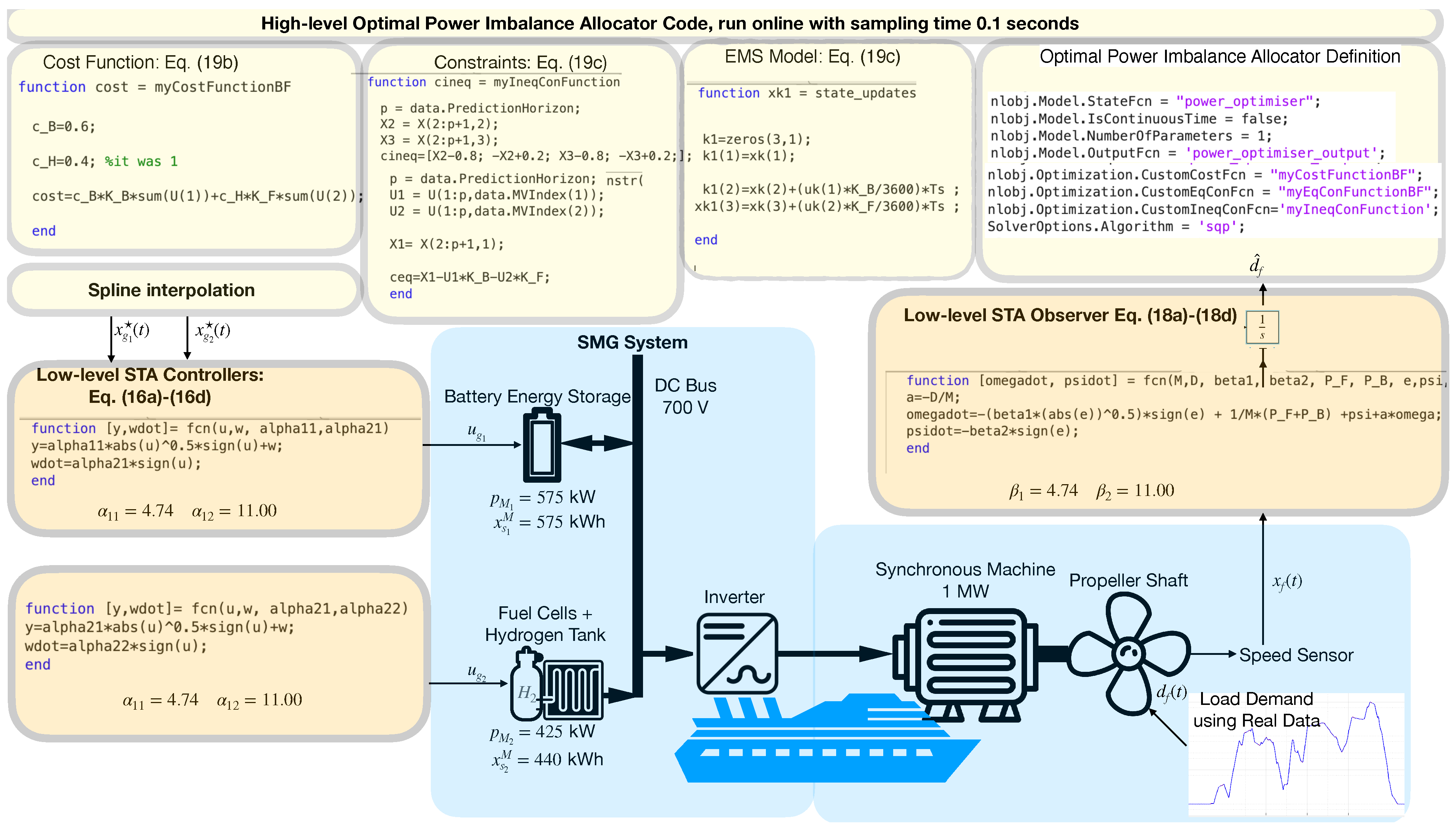
  • Low-Level STA Controller:
    σ g ( t ) : = x g ( t ) x g ( t )
    u g ( t ) : = u g 1 ( t ) + u g 2 ( t )
    u g 1 ( t ) : = Col ( α 1 i | σ g i ( t ) | 1 2 sign ( σ g i ( t ) ) )
    u ˙ g 2 ( t ) : = Col ( α 2 i sign ( σ g i ( t ) ) )
  • Low-Level STA Observer
    e f ( t ) : = x ^ f ( t ) x f ( t )
    x ^ ˙ f ( t ) = r f x f ( t ) + 1 x g ( t ) β 1 | e f ( t ) | 1 2 sign ( e f ( t ) ) + w f ( t )
    w ˙ f ( t ) = β 2 sign ( e f ( t ) )
    d ^ f = w f ( t )
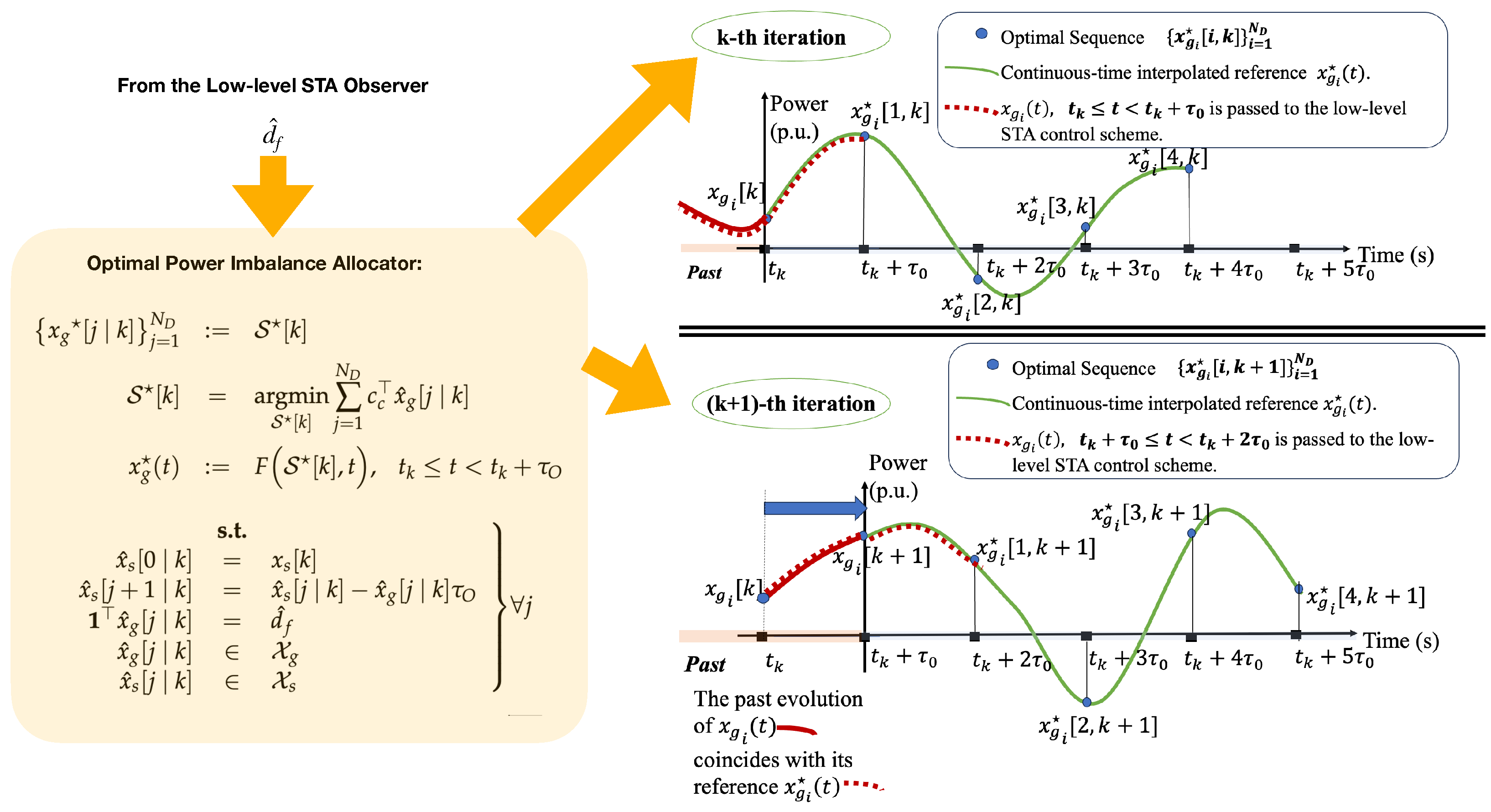
  • High-Level Optimal Power Imbalance Allocator:
    x g [ j | k ] j = 1 N D : = S [ k ]
    S [ k ] = argmin S [ k ] j = 1 N D c c x ^ g [ j | k ] x g ( t ) : = F S [ k ] , t , t k t < t k + τ O
    s . t . x ^ s [ 0 | k ] = x s [ k ] x ^ s [ j + 1 | k ] = x ^ s [ j | k ] x ^ g [ j | k ] τ O 1 x ^ g [ j | k ] = d ^ f x ^ g [ j | k ] X g x ^ s [ j | k ] X s j
The positive constants α 1 i , α 2 i in (17c) and (17d) are α 1 i = 1.5 Δ h i , α 2 i = 1.1 Δ h i , where Δ h i is a known positive constant [27]; x ^ f ( t ) is an estimate of x f ( t ) ; β 1 , β 2 in (18b)–(18d) are positive design constants; and the vector matrix c c : = Col ( c c i ) , c c R N represents the unit cost of consumption associated with each ESS. Note that the condition x ^ s [ 0 | k ] = x s [ k ] in Equation (19c) initialises the prediction series of x ^ s with the measurement of the actual consumption at the instant t k . This initialisation serves as a starting point for iteratively solving the online optimisation problem. Inspired by the principle of receding horizon, we only pass the interpolated reference x g ( t ) to the low-level controllers only for the first τ O seconds, as per (19c), where F ( · ) represents the interpolating function. This principle is visually represented and illustrated in Figure 2, where a single i-th component of x g ( t ) is considered for graphical representation.
The main key finding of this article is stated in the following Theorem:
Theorem 1. 
Under Assumptions 1 and 2, the following conditions hold:
(I) 
The low-level STA observer is capable of estimating the unknown load power demand d f in a finite time t f .
(II) 
Provided that each entry of the unit cost vector c c satisfies
c c i c c n i = 1 , , N , n = 1 , , N , s . t . i n
where i , n are positive distinct integers, at each iteration, there exists a unique optimal sequence S [ k ] solving the optimisation problem (19a)–(19c).
(III) 
The low-level STA controllers are capable of driving x g ( t ) to x g ( t ) in a finite time t g and of dynamically tracking its smooth evolution over time.
Proof. 
Proof of Part (I)—Solving Objective 1: We subtract (5) from (18b), and the STA observer error dynamics hold:
e ˙ f ( t ) = β 1 | e f ( t ) | 1 2 sign ( e f ( t ) ) + w f ( t ) + d f
w ˙ f ( t ) = β 2 sign ( e f ( t ) )
If we introduce an auxiliary error variable e f 2 ( t ) : = w f ( t ) + d f , we write the error system as:
e ˙ f ( t ) = β 1 | e f ( t ) | 1 2 sign ( e f ( t ) ) + e f 2 ( t ) e ˙ f 2 ( t ) = β 2 sign ( e f ( t ) )
The system in (22) is finite-time stable β 1 , β 2 > 0 [27], which means that the conditions e f = e f 2 = 0 hold in a finite time t f . When e f 2 = 0 , an accurate estimate d ^ f for d f can be extracted in real time from the observer variable d ^ f = w f ( t ) . Note that the STA observer can also estimate online the non-constant power load demand d f ( t ) , provided that | d ˙ f ( t ) | < Δ f . This is achieved by tuning the two gains β 1 = 1.5 Δ f , β 2 = 1.1 Δ f [27].
Proof of Part (II)—Solving Objective 2
Under Assumption 2(A3), at every time instant t k , there is always a feasible solution S [ k ] that satisfies the constraint (19c). We now prove that if c c satisfies (20) at each iteration, there exists a unique optimal S [ k ] that solves the optimisation problem. Since constraints (19c) create a bounded region, the minimum of the objective function exists within this region. By exploiting the constraint on power imbalance 1 x ^ g [ j | k ] = d ^ f , we can express an arbitrarily chosen n-th component of x ^ g [ j , k ] as
x ^ g n [ j | k ] = d ^ f 1 x ^ g n [ j | k ]
where the vector x ^ g n R N 1 is built from x ^ g [ i | k ] by removing the n-th entry. If we substitute (23) into the cost function (19b), we can rewrite the high-level optimal power imbalance allocator problem in a simpler form as:
S [ k ]   =   argmin S [ k ] j = 1 N D ( c c c c n 1 ) x ^ g [ j | k ] + c c n d ^ f
s . t . x ^ s [ 0 | k ] = x s [ k ] x ^ s [ j + 1 | k ] = x ^ s [ j | k ] x ^ g [ j | k ] τ O x ^ g [ j | k ] X g x ^ s [ j | k ] X s j
Let us isolate the individual j-th contribution of the cost function
J ( x ^ g [ j | k ] ) : = ( c c c c n 1 ) x ^ g [ j | k ] + c c n d ^ f
Suppose, for the sake of contradiction, that there are two distinct solutions x ^ g ( 1 ) [ j | k ] and x ^ g ( 2 ) [ j | k ] , both minimising the objective function (26). Since the minimum exists, both J ( x ^ g ( 1 ) [ j | k ] ) and J ( x ^ g ( 2 ) [ j | k ] ) have the same minimum value, which means that
( c c c c n 1 ) x ^ g ( 1 ) [ j | k ] x ^ g ( 2 ) [ j | k ] = 0
As x ^ g ( 1 ) [ j | k ] and x ^ g ( 1 ) [ j | k ] are distinct,
i : x ^ g i ( 1 ) [ j | k ] x ^ g i ( 2 ) [ j | k ]
However, since c c satisfies (20), to enforce (27), we need to ensure
( c c i c c c n ) x ^ g i ( 1 ) [ j | k ] x ^ g i ( 2 ) [ j | k ] = 0
This can only be possible if
x ^ g i ( 1 ) [ j | k ] = x ^ g i ( 2 ) [ j | k ]
which clearly contradicts (28); therefore, x ^ g ( 1 ) [ j | k ] must coincide with x ^ g ( 2 ) [ j | k ] , which proves the uniqueness of the minimum. Therefore, it is always possible to find a minimum x g [ j | k ] for J ( x ^ g [ j | k ] ) using linear programming [28].
Two situations can occur:
(a)
If during the time horizon of τ D seconds, the evolution of x ^ s [ j | k ] does not breach any of its associated constraints as per (19c), then the minimum x g [ j | k ] for J ( x ^ g [ j | k ] ) will also minimise the overall cost function (19b). A series S [ k ] composed of N D identical references will be generated and interpolated via the interpolator (19c).
(b)
If at a generic m-th step, the boundaries for the energy storage x ^ s [ m | k ] are reached, these can be reflected by constraining the associated output powers to be equal to zero, hence obtaining a different hyper-rectangle redefining the boundaries of x ^ g [ m | k ] and finding another single minimum for the cost function. A series S [ k ] composed of N D nonidentical references will be generated and interpolated via the interpolator (19c).
Proof of Part (III)—Solving Objective 3
We show that our STA controller drives x g ( t ) towards an interpolated reference x g ( t ) in finite time t g . To derive a suitable state-space representation to analyse the stability, we introduce the error variable
σ g 2 ( t ) : = A g σ g ( t ) + B g u 2 g ( t ) + B g d g ( t ) + x ˙ g ( t ) ,
which yields
σ ˙ g ( t ) = σ g 2 ( t ) + B g u g 1 ( t )
σ ˙ g 2 ( t ) = h ( σ g ( t ) ) + B g u ˙ g 2 ( t )
Each i-th component of the system (32a) and (32b) is in the form
σ ˙ g i ( t ) = σ g 2 i ( t ) B g i α 1 i | σ g i ( t ) | 1 2 sign ( σ g i ( t ) )
σ ˙ g 2 i ( t ) = h i ( σ g i ( t ) ) B g i α 2 i sign ( σ g i ( t ) )
The system (33a) and (33b) is in the standard form of the perturbed STA algorithm [27]. Under Assumption 2 and given A g Hurwitz, the matched disturbance h i ( σ g i ( t ) ) is composed of a sum of bounded terms by direct calculation and is therefore bounded, which means that | h i ( σ g i ( t ) ) | < Δ h i , where Δ h i is an a priori known positive constant. If [27]
α 1 i = 1.5 Δ h i α 2 i = 1.1 Δ h i
the system (33a) and (33b) reaches the origin in a finite time t g , guaranteeing the achievement of Objective 3. When the system (33a) is restricted to stay on the sliding surface σ g i ( t ) , the STA control action compensates in real time the influence of the matched disturbance h i ( σ g i ( t ) ) and therefore remains completely insensitive to the disturbance d g i ( t ) and to possible bounded and known variations of x g ( t ) .
The aforementioned arguments prove the Theorem. □
Remark 4. 
If there exists at least a unit cost c c m such that c c i = c c n , it implies that the objective function assigns the same weight or importance to different decision variables. This, in turn, leads to the existence of multiple solutions that achieve the same minimum objective function value. In other words, the uniqueness of the solution is compromised, as there may be alternative solutions with identical objective values.
Remark 5. 
The use of interpolation is mandatory to combine the effect of high- and low-level loops. For the existence of the sliding mode, it is necessary to ensure that the optimal generated reference x g ( t ) is differentiable with respect to time. In this article, we use the STA controller; the first and second time derivative of σ g ( t ) must exist [29]. Therefore, a quadratic spline should be generated from the discontinuous optimal series.
Remark 6. 
Note that in this article, we separately analysed the stability of the three schemes according to the following conditions: the matrix A g is Hurwitz and any variation in x g is considered as a matched bounded disturbance by the STA low-level controller; the convergence of the STA observer is decoupled from the STA low-level controller by virtue of the underlying structure of the dynamics of the SMG system.

5. Simulation

We consider an SMG composed of N = 2 ESSs, that is, a BESS (numbered ESS1), which belongs to the subset N r and an FC (numbered ESS2) which belongs to the subset N c . We consider an SMG of 1 (MW) rated power, which is also set to be the base power for the per unit (p.u) parameters. We set p m 1 = p M 1 = 0.575 ( p . u . ) , p M 2 = 0.425 ( p . u . ) , x s 1 M = 0.575 ( p . u . h ) , x s 2 M = 0.44 ( p . u . h ) . These parameters are selected in accordance with the data made available via the acknowledged Innovate UK grant with industry partners. We employ widely accepted model parameters found in the existing literature [2] for the representation of the SMG state space, which are a g 1 = 10 , a g 2 = 3.87 , b g 1 = 10 , b g 2 = 3.87 , r f = 0.60 . We consider Δ h = Δ f = 10 , and we set the parameters of the STA controllers as α 1 1 = α 1 2 = 4.74 , α 2 1 = α 2 2 = 11.00 . The unit costs of consumption are selected as c c 1 = 0.60 , c c 2 = 0.40 . The STA observer design constants are set as β 1 = 4.74 , β 2 = 11.00 . We numerically estimate the values for t g and t f following the methodology presented in [27], obtaining t g = t f = 0.15 s. The STA observer and controllers are implemented in a MATLAB-Simulink environment using the Euler method with an integration step of 0.1 ms. The simulations run for a duration of T s i m = 1200 s. If we consider (14), max ( t g , t f ) = 0.15 s, then τ O 0.15 . Therefore, the power imbalance allocator scheme is executed with a sampling time of τ O = 10 s. The optimisation problem (19a)–(19c) is implemented using the dedicated MATLAB Optimisation Toolbox and the algorithm Fmincon Sequential Quadratic Programming (SQP). Figure 3 shows an extract of the implementation of the MATLAB-Simulink code of the strategy proposed in this paper, following the architecture in Figure 1. In particular, the technical values of the considered SMG are given, along with the MATLAB R2023b functions architecture of the two-level control strategy.
We consider four scenarios:
  • Scenario PI: an arbitrarily defined power imbalance allocator is imposed to determine the power reference for each ESS, i.e., x g : = κ d ^ f , κ : = [ κ 1 , κ 2 ] , κ 1 = p M 1 , κ 2 = p M 1 Furthermore, during this scenario, each ESS is regulated via conventional PI controller.
  • Scenario PIO: during which our optimal power imbalance allocator is utilised, and each ESS is regulated via PI controllers. The proportional and integral gains for the PI controllers are set equal to −1.
  • Scenario SM: the arbitrary power allocator defined in the scenario PI is used and each ESS is regulated via STA controllers.
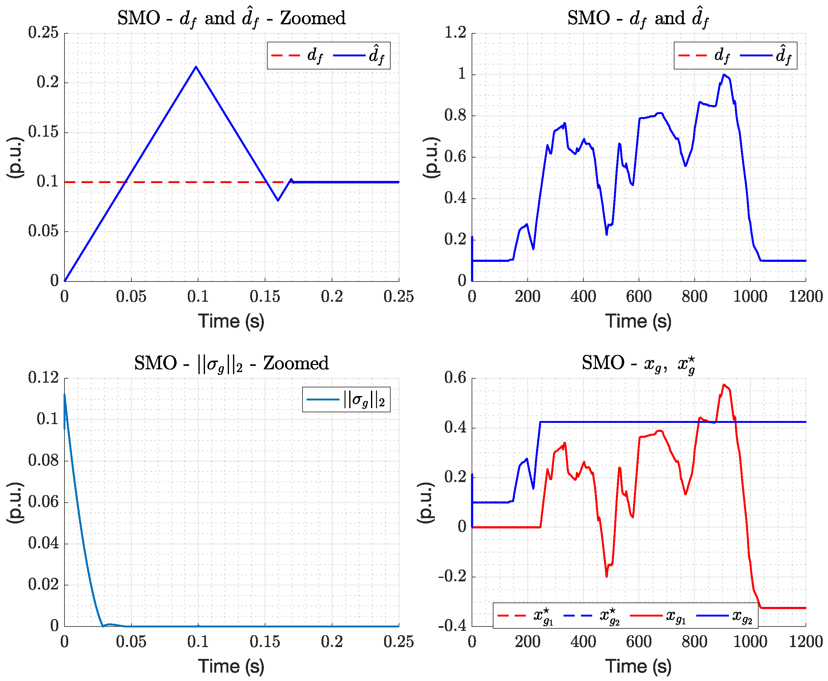
  • Scenario SMO: the proposal of this paper, where the optimal power imbalance allocator is used in conjunction with STA controllers.
We define the integral metric:
J : = 0 T s i m J ( x g ( τ ) ) d τ
which represents the total operational cost of the SMG within the simulation time horizon.
Figure 4 shows the results of the simulation carried out. In Scenario PI, there is an arbitrarily defined power split and the frequency deviation is acceptably regulated, whilst the operational cost is not minimised. If we use our optimal power imbalance allocator together with standard PI control (Scenario PIO), we can achieve an important cost reduction; however, the frequency deviation is still only acceptably regulated (see the frequency deviation figure of Scenario PIO). By virtue of the STA property, we can ensure excellent frequency regulation in Scenario SM and also minimise the operational cost in Scenario SMO. This scenario, which represents the proposal of this article, shows excellent speed regulation properties while reducing the total operational cost J by 22%. In this scenario, when load demand is low, ESS2 is used to charge ESS1. Note that in scenario SM, as there is no high-level scheme with the associated interpolation architecture communicating changes in load demand, the frequency deviation always remains equal to zero. On the other hand, in the SMO scenario, we observe a small frequency deviation only when the unknown load power demand d f varies over time. These frequency deviations are much smaller than the one obtained in Scenario PIO, which demonstrated the better performance of the STA algorithm compared to the PI algorithm. To further compare the scenarios analysed, it is worth noting that Scenario PIO and Scenario SMO are characterised by identical cost J . Nevertheless, the low-level STA controllers adopted in Scenario SMO better track the optimal reference when compared to standard PI controllers. This fact can be observed by analysing the frequency deviation x f in scenario PIO and SMO.
The excellent performance of the STA-based algorithms is summarised in Figure 5. It is possible to see that condition d ^ f = d f is enforced in less than 0.20 s and is maintained throughout the simulation horizon. As also proven in the paper, σ g ( t ) converges to zero in finite time, guaranteeing that x g ( t ) tracks the optimal time-varying reference x g ( t ) .

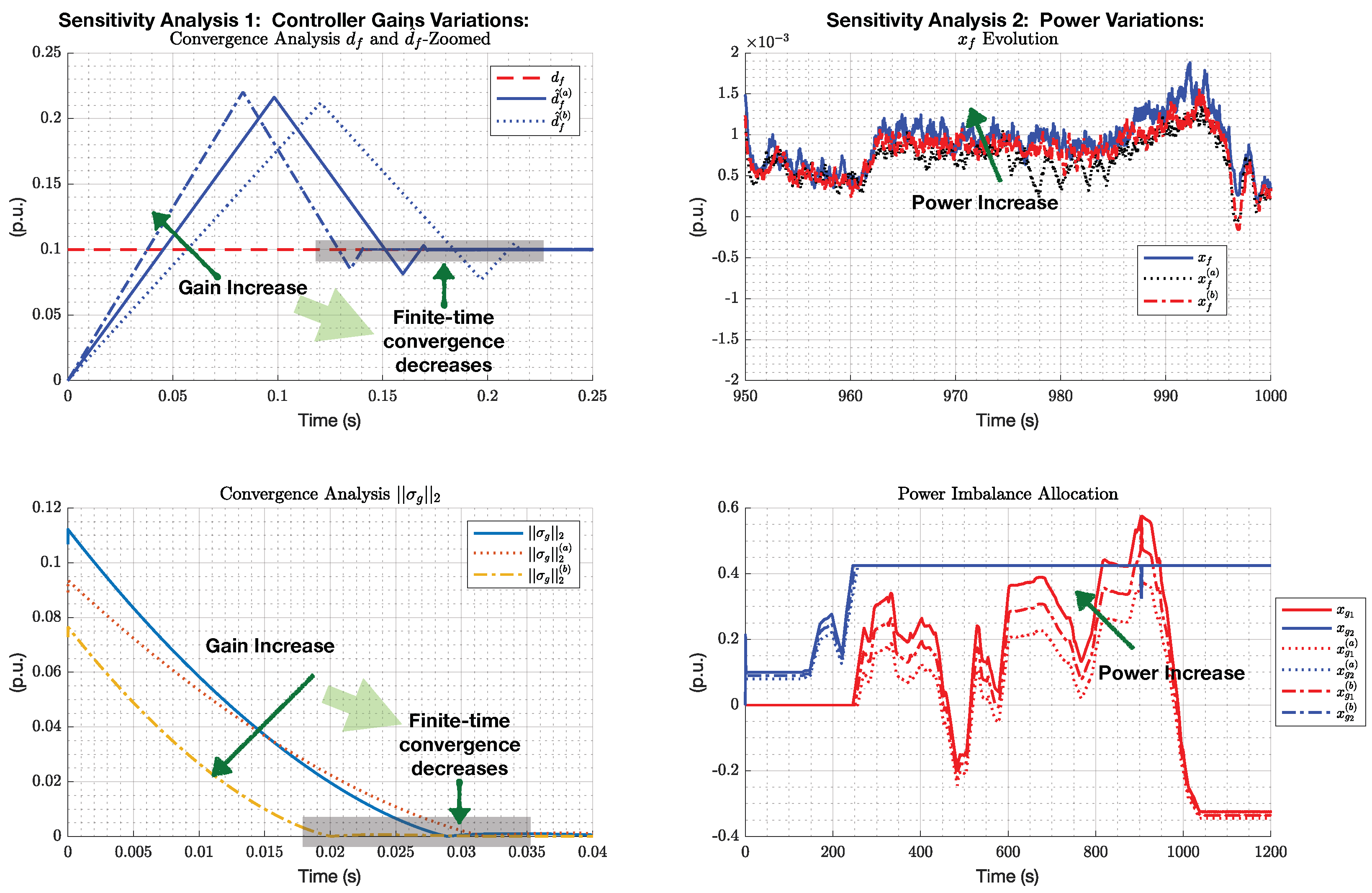
5.1. Sensitivity Analysis

In order to further assess the performance of the Scenario SMO, two sensitivity analyses are conducted, which examine, respectively, changes to the controllers and observer gains and to the power load demand.

5.1.1. Sensitivity Analysis 1

Sensitivity Analysis 1 investigates the impact of variations in the design parameters of both the low-level STA observer and the low-level STA controllers. The adjustments focus on the gains, modified as follows:
α ˜ 1 1 = χ α 1 1 α ˜ 1 2 = χ α 1 2 α ˜ 2 1 = χ α 2 1 α ˜ 2 2 = χ α 2 2 β ˜ 1 = χ β 1 β ˜ 2 = χ β 2
Here, ˜ denotes the scaled gain, and the scaling factor χ ranges from 0.8 to 1.2 . Following the insights in [27], the convergence time T STA —the time of the STA algorithm for both controllers and observer—achieves sliding motion proportional to χ , as is also numerically demonstrated in Figure 6. Notably, the proof of Theorem 1 confirms that sliding motion is maintained for gain adjustments within the specified range, thus ensuring system stability under both under- and over-tuning conditions.

5.1.2. Sensitivity Analysis 2

This sensitivity analysis considers variations in the power load demand d f as follows:
d ˜ f = χ d f
where d ˜ f is a scaled version of d f , and the scaling factor χ ranges from 0.8 to 1.2 as above. From Figure 6, it is possible to appreciate that the proposed scheme is also still able to optimally allocate the power imbalance between the BESS and the FC under such conditions. The simulation also reveals that the small frequency oscillations, which are caused by the time-varying feature of the power demand, are not sensibly affected by the scaling of d f .
Remark 7. 
Note that, in the event of communication failures in measuring the state vector x s ( t ) , Scenario PI and Scenario SM can be used to still achieve frequency regulation via the arbitrarily defined power imbalance allocator defined above. In such a scenario, the low-level STA controllers are still capable of maintaining stable operations on the SMG but without minimising the operational costs.

6. Conclusions

This paper has introduced an original two-level control strategy for SMGs, with a focus on optimising power allocation and achieving precise asymptotic frequency regulation. Drawing inspiration from the STA, we have integrated a state observer into our system to rapidly estimate power load demand imbalances. Our online optimal methodology has been designed to establish power references for individual ESSs, while decentralised low-level STA control guarantees finite-time reference tracking. The evidence from our extensive numerical simulations highlighted the exceptional ability of our proposal to regulate frequency with precision and significantly reduce operational costs. This paper lay the foundation for future high-impact research directions. A first expansion can be centred on the ship platoon scenarios, where multiple SMGs collaborate under suitable communication protocols to achieve common optimisation objectives. A second expansion can be focussed on experimental validation through application to more complex SMGs, utilising a real setup provided by our industry partners. These two prospects underscore the importance and applicability of our proposal, promising significant advancements in this research field.

Author Contributions

Conceptualization, G.R. and D.K.B.; methodology, G.R.; software, G.R.; validation, G.R., D.K.B. and P.P.M.; formal analysis, G.R.; investigation, G.R.; resources, G.R. and D.K.B.; data curation, G.R.; writing—original draft preparation, G.R. and D.K.B.; writing—review and editing, P.P.M.; visualization, G.R.; supervision, P.P.M.; project administration, G.R.; funding acquisition, P.P.M. All authors have read and agreed to the published version of the manuscript.

Funding

This research was partially supported by the Innovate UK Project Clean Maritime Demonstration Competition Round 2 (CMDC2), Project ZERO—Zero Emission Research and Offshore Service Vessel, Grant 10039625. The APC is paid by University of Exeter. For the purpose of open access, the author has applied a ‘Creative Commons Attribution (CC BY) licence to any Author Accepted Manuscript version arising from this submission.

Data Availability Statement

The data presented in this study are available on request from the corresponding author.

Conflicts of Interest

The authors declare no conflicts of interest.

Abbreviations

The following abbreviations are used in this manuscript:
STASuper-Twisting Algorithm
ESSEnergy Storage System
SMGShipboard Microgrid
LFCLoad Frequency Control
BESSBattery Energy Storage System
FCFuel Cell
EMSEnergy Management System

References

  1. International Maritime Organization. Fourth Greenhouse Gas Study; International Maritime Organization: London, UK, 2020. [Google Scholar]
  2. Yildirim, B.; Gheisarnejad, M.; Khooban, M.H. Delay-dependent stability analysis of modern shipboard microgrids. IEEE Trans. Circuits Syst. I Regul. Pap. 2021, 68, 1693–1705. [Google Scholar] [CrossRef]
  3. Xu, L.; Guerrero, J.M.; Lashab, A.; Wei, B.; Bazmohammadi, N.; Vasquez, J.C.; Abusorrah, A. A review of DC shipboard microgrids—Part I: Power architectures, energy storage, and power converters. IEEE Trans. Power Electron. 2021, 37, 5155–5172. [Google Scholar] [CrossRef]
  4. Feng, X.; Butler-Purry, K.L.; Zourntos, T. Real-time electric load management for DC zonal all-electric ship power systems. Electr. Power Syst. Res. 2018, 154, 503–514. [Google Scholar] [CrossRef]
  5. Aboelezz, A.M.; Sedhom, B.E.; El-Saadawi, M.M.; Eladl, A.A.; Siano, P. State-of-the-Art Review on Shipboard Microgrids: Architecture, Control, Management, Protection, and Future Perspectives. Smart Cities 2023, 6, 1435–1484. [Google Scholar] [CrossRef]
  6. Hassan, M.A.; Su, C.L.; Pou, J.; Sulligoi, G.; Almakhles, D.; Bosich, D.; Guerrero, J.M. Dc shipboard microgrids with constant power loads: A review of advanced nonlinear control strategies and stabilization techniques. IEEE Trans. Smart Grid 2022, 13, 3422–3438. [Google Scholar] [CrossRef]
  7. Vafamand, N.; Khooban, M.H.; Dragičević, T.; Boudjadar, J.; Asemani, M.H. Time-delayed stabilizing secondary load frequency control of shipboard microgrids. IEEE Syst. J. 2019, 13, 3233–3241. [Google Scholar] [CrossRef]
  8. Yuan, Z.L.; Zhang, C.K.; Shangguan, X.C.; Jin, L.; Xu, D.; He, Y. Stability analysis of load frequency control for shipboard microgrids with occasional large delays. IEEE Trans. Circuits Syst. II Express Briefs 2021, 69, 2161–2165. [Google Scholar] [CrossRef]
  9. Xi, K.; Dubbeldam, J.L.; Lin, H.X.; van Schuppen, J.H. Power-imbalance allocation control of power systems-secondary frequency control. Automatica 2018, 92, 72–85. [Google Scholar] [CrossRef]
  10. Rinaldi, G.; Menon, P.P.; Edwards, C.; Ferrara, A. Sliding mode observer-based finite time control scheme for frequency regulation and economic dispatch in power grids. IEEE Trans. Control Syst. Technol. 2021, 30, 1296–1303. [Google Scholar] [CrossRef]
  11. Zia, M.F.; Elbouchikhi, E.; Benbouzid, M. Microgrids energy management systems: A critical review on methods, solutions, and prospects. Appl. Energy 2018, 222, 1033–1055. [Google Scholar] [CrossRef]
  12. Zhao, C.; Mallada, E.; Dörfler, F. Distributed frequency control for stability and economic dispatch in power networks. In Proceedings of the 2015 American Control Conference (ACC), Chicago, IL, USA, 1–3 July 2015; pp. 2359–2364. [Google Scholar]
  13. Shankar, R.; Chatterjee, K.; Chatterjee, T. Coordination of economic load dispatch and load frequency control for interconnected power system. J. Inst. Eng. (India) Ser. B 2015, 96, 47–54. [Google Scholar] [CrossRef]
  14. Drakunov, S.V.; Utkin, V.I. Sliding mode control in dynamic systems. Int. J. Control 1992, 55, 1029–1037. [Google Scholar] [CrossRef]
  15. Castillo, I.; Fridman, L.; Moreno, J.A. Super-twisting algorithm in presence of time and state dependent perturbations. Int. J. Control 2018, 91, 2535–2548. [Google Scholar] [CrossRef]
  16. Nagesh, I.; Edwards, C. A multivariable super-twisting sliding mode approach. Automatica 2014, 50, 984–988. [Google Scholar] [CrossRef]
  17. Kali, Y.; Saad, M.; Benjelloun, K.; Khairallah, C. Super-twisting algorithm with time delay estimation for uncertain robot manipulators. Nonlinear Dyn. 2018, 93, 557–569. [Google Scholar] [CrossRef]
  18. Machado, J.E.; Rinaldi, G.; Cucuzzella, M.; Menon, P.P.; Scherpen, J.M.; Ferrara, A. Online Parameters Estimation Schemes to Enhance Control Performance in DC Microgrids. Eur. J. Control 2023, 74, 100860. [Google Scholar] [CrossRef]
  19. Incremona, G.P.; Ferrara, A.; Magni, L. Hierarchical model predictive/sliding mode control of nonlinear constrained uncertain systems. IFAC PapersOnLine 2015, 48, 102–109. [Google Scholar] [CrossRef]
  20. Incremona, G.P.; Cucuzzella, M.; Magni, L.; Ferrara, A. MPC with sliding mode control for the energy management system of microgrids. IFAC PapersOnLine 2017, 50, 7397–7402. [Google Scholar] [CrossRef]
  21. Palmieri, A.; Rosini, A.; Procopio, R.; Bonfiglio, A. An MPC-sliding mode cascaded control architecture for PV grid-feeding inverters. Energies 2020, 13, 2326. [Google Scholar] [CrossRef]
  22. Bahrampour, E.; Dehghani, M.; Asemani, M.H.; Abolpour, R. Load frequency fractional-order controller design for shipboard microgrids using direct search alghorithm. IET Renew. Power Gener. 2023, 17, 894–906. [Google Scholar] [CrossRef]
  23. Khooban, M.H.; Dragicevic, T.; Blaabjerg, F.; Delimar, M. Shipboard microgrids: A novel approach to load frequency control. IEEE Trans. Sustain. Energy 2017, 9, 843–852. [Google Scholar] [CrossRef]
  24. Liu, B.; Song, Z.; Yu, B.; Yang, G.; Liu, J. A Feedforward Control-Based Power Decoupling Strategy for Grid-Forming Grid-Connected Inverters. Energies 2024, 17, 424. [Google Scholar] [CrossRef]
  25. Magni, L.; Scattolini, R. Model predictive control of continuous-time nonlinear systems with piecewise constant control. IEEE Trans. Autom. Control 2004, 49, 900–906. [Google Scholar] [CrossRef]
  26. Bejestani, A.K.; Annaswamy, A.; Samad, T. A hierarchical transactive control architecture for renewables integration in smart grids: Analytical modeling and stability. IEEE Trans. Smart Grid 2014, 5, 2054–2065. [Google Scholar] [CrossRef]
  27. Moreno, J.A.; Osorio, M. Strict Lyapunov functions for the super-twisting algorithm. IEEE Trans. Autom. Control 2012, 57, 1035–1040. [Google Scholar] [CrossRef]
  28. Bertsimas, D.; Tsitsiklis, J.N. Introduction to Linear Optimization; Athena Scientific: Belmont, MA, USA, 1997; Volume 6. [Google Scholar]
  29. Chalanga, A.; Kamal, S.; Fridman, L.M.; Bandyopadhyay, B.; Moreno, J.A. Implementation of super-twisting control: Super-twisting and higher order sliding-mode observer-based approaches. IEEE Trans. Ind. Electron. 2016, 63, 3677–3685. [Google Scholar] [CrossRef]
Figure 1. The considered architecture for the SMG, with the depiction of the low-level STA observer and the local low-level STA controllers, along with the high-Level optimal power imbalance allocator.
Energies 17 01703 g001
Figure 2. A visual interpretation of the optimised interpolated reference x g ( t ) generated iteratively using the high-level optimal power imbalance allocator. The representation focusses on the i-th scalar component of x g ( t ) .
Energies 17 01703 g002
Figure 3. A schematic of the considered SMG composed of a BESS and a FC. The technical details of the nominal power-energy storage capacity of the SMG are also reported. An extract of the MATLAB-based code implementation of the low-level STA observer, of the optimal power imbalance allocator, and of the low-level STA controllers are also illustrated.
Energies 17 01703 g003
Figure 4. From Left to right: Time histories of the power balance with x g 1 , x g 2 , x g 3 ; the frequency deviation x f ; the consumption variables x c 1 and x c 2 ; and the cost metric J for the four scenarios PI, PIO, SM, and SMO in each row of the figure.
Energies 17 01703 g004
Figure 5. (Top): Time histories of the power load demand d f and its estimate d ^ f obtained via the proposed STA observer, with a zoomed view during the first 0.25 s to show the convergence in finite time. (Bottom): Time histories of | | σ g | | 2 during the first 0.25 s and time histories of the ESS output power x g ( t ) and its actual value x g ( t ) .
Energies 17 01703 g005
Figure 6. Two sensitivity analyses of the algorithm proposed in this paper. (Sensitivity Analysis 1): Time histories of d f and their estimates when the gains b e t a 1 , β 2 are scaled and the numerical evaluation of the finite-time convergence. Time histories of | | σ | | 2 of the low-level STA controllers when the gains α 1 i , α 2 i are scaled and the impact of the finite-time convergence. (Sensitivity Analysis 2): Time histories of the frequency deviation x f when the power demand d f is scaled. Time histories of the ESS output power x g ( t ) when the power demand is scaled.
Energies 17 01703 g006
Table 1. List of symbols and variables adopted in the article.
SymbolPhysical Meaning and Measurement Unit
x g i ( t ) ESS output power   (p.u.)
x g i ( t ) ESS output power optimal reference   (p.u.)
x s i ( t ) , x ^ s i [ k ] ESS energy storage level and its discrete time prediction   (p.u. s)
u g i ( t ) ESS low-level control   (p.u.)
d f , d ^ f   Power load demand and its estimate   (p.u.)
x f ( t ) Frequency deviation   (p.u.)
Disclaimer/Publisher’s Note: The statements, opinions and data contained in all publications are solely those of the individual author(s) and contributor(s) and not of MDPI and/or the editor(s). MDPI and/or the editor(s) disclaim responsibility for any injury to people or property resulting from any ideas, methods, instructions or products referred to in the content.

