Hybrid Metaheuristic Algorithms for Optimization of Countrywide Primary Energy: Analysing Estimation and Year-Ahead Prediction

Abstract

In the present work, India’s primary energy use is analysed in terms of four socio-economic variables, including Gross Domestic Product, population, and the amounts of exports and imports. Historical data were obtained from the World Bank database for 44 years as annual values (1971–2014). Energy use is analysed as an optimisation problem, where a unique ensemble of two metaheuristic algorithms, Grammatical Evolution (GE), and Differential Evolution (DE), is applied. The energy optimisation problem has been investigated in two ways: estimation and a year-ahead prediction. Models are compared using RMSE (objective function) and further ranked using the Global Performance Index (GPI). For the estimation problem, RMSE values are found to be as low as 0.0078 and 0.0103 on training and test datasets, respectively. The average estimated energy use is found in good agreement with the data (RMSE = 6.3749 kgoe/capita), and the best model (E10) has an RMSE of 5.8183 kgoe/capita, with a GPI of 1.7249. For the prediction problem, RMSE is found to be 0.0096 and 0.0122 on training and test datasets, respectively. The average predicted energy use has RMSE of 7.8857 (kgoe/capita), while Model P20 has the best value of RMSE (7.9201 kgoe/capita) and a GPI of 1.8836.

1. Introduction

Energy forms the basis of our lives, is central to a country’s economy, and is the primary requirement for every organism thriving on the planet. Economic and population growth has directly correlated to the energy demand [1]. Therefore, energy planning and development, research, and modelling have become a dedicated part of organizations to provide future generations with energy security. The depletion of oil and coal-based conventional fuels has also forced the human race to shift the focus on renewable energy sources and to adapt to energy-responsible behaviour.

India is a developing country with a rapid pace of industrial expansion and infrastructural development, coupled with an increasing population (1.4 billion people), which, consequently, leads to high energy demand. A few decades ago, on average, India’s industrial sector consumed 52% of the energy, while the transportation and domestic sectors accounted for 23% and 11%, respectively [2]. Furthermore, the evolution of the modern lifestyle, characterised by the use of electrical and electronic devices, has been pursued for greater comfort and enjoyment [3]. Primary energy use in India, in the decade after 2009, increased from 21 EJ to 34 EJ, a rise of 62% in only a decade, with an average growth rate of 4.7% [4]. At this rate, the energy supply needs to grow to meet the future energy demand [5].

Therefore, India needs to address its energy challenge through technological development and policy changes to include the options available within the energy sectors and accelerate toward achieving net-zero emissions by 2050. For this, estimating energy use to assess the growth of energy demand is an essential activity in drafting future policies.

Energy demand forecasting involves using long-term historical data to predict future energy demand using statistical methods [6]. These forecast models often depend on climate, socio-economic parameters, and demographic data, resulting in high uncertainties in the predicted results. These variations occur when projections are made at different scales. Researchers have extensively studied energy demand estimation and prediction problems across various time frequencies and scales (daily, monthly, and annual), combined with sectoral and regional levels, as well as the country as a whole (usually referred to as “primary energy demand”).

These modelling approaches to the problems of energy demand estimation and prediction can be classified into three main categories, viz, (i) statistical methods and time-series models, (ii) econometric models, and (iii) Artificial Intelligence (AI) methods [7,8]. Further AI methods have been developed by neuro-fuzzy methods and, more recently, metaheuristics [9,10,11].

AI techniques have been developed and implemented to solve energy demand forecasting problems. These provide greater accuracy in comparison to statistical/deterministic means. Therefore, recently, the available literature has focused more on developing these methods. In this section, we look at some of the approaches in recent years. Jiang et al. [1] presented a new method to forecast short-term electrical energy demand, combining adaptive Fourier decomposition and a new signal pre-processing technology that extracts the helpful element from the electricity demand data series by discarding the noise. They suggested that the method developed using pre-processing data to remove seasonality can be effectively used to forecast energy demand. Sajadi et al. [12] investigated the effect of energy prices on long-term energy forecasting. In addition, they studied the electricity generation from natural gas, which has been reported missing in the literature. They applied an approach to first-order Takagi–Sugeno type fuzzy inference systems (TS-FIS) to construct the regression models. Application of the developed model was exhibited through the case study of Iran, and it was deduced that high electricity prices result in considerably less energy use. In a similar study, Dalfard et al. [13] investigated the relationship between the hike in energy prices with the electricity demand and the use of natural gas. Adaptive Network-based FIS (ANFIS) combined with Monte Carlo simulation was developed to model natural gas consumption in power generation (NGPG). The approach was verified using data on electrical energy and natural gas combined with socio-economic parameters for Iran between 2010 and 2016. It was reported that the approach developed could be adopted for prediction problems where the energy prices suddenly vary. Daş [14] forecasted Turkey’s energy demand using Particle Swarm Optimization with mutation based on an improved neural network (PSOM-NN). Energy demand was modelled in terms of Turkey’s GDP, population, imports, and exports between 1979 and 2005. It was concluded that the PSOM-NN produces better forecasts with greater accuracy when compared to previous approaches for modelling energy demand. Salcedo-Sanz et al. [15] described the one-year-ahead energy demand estimation approach for Spain, using two different computational algorithms, described as a modified Harmony Search (HS) optimization algorithm with an exponential prediction model and an Extreme Learning Machine (ELM). Data for 14 macroeconomic variables for 30 years were used to model the energy demand. When compared with the previously published algorithms, the prediction accuracy was reported to improve the results by 15%. The results were extended to model CO₂ emissions for the country using the same evolutionary algorithms, and the accuracy was reported to improve by 10%. Sánchez-Oro et al. [16] presented the hybrid neighbourhood variable search–Extreme Learning Machine algorithm to predict the energy demand for Spain. The feature selection mechanism combined with the exponential prediction model using the historical data for several macroeconomic variables resulted in an excellent performance of the proposed approach. It was further testified that even during the crisis year of 2008, the energy prediction was accurate within 2%. Toksar [17] applied Ant Colony Optimization (ACO) for Turkey’s energy demand estimation using the four commonly used socio-economic variables (GDP, population, imports, and exports). Two models (linear and quadratic) were proposed, and the ACO optimized both. It was concluded that the quadratic ACO model outperforms the linear model and has an accuracy of as low as −0.15% relative error. Unler [18], in a similar approach to Turkey, presented a swarm intelligence approach to estimate the energy demand using the data for macroeconomic variables (GDP, population, imports, and exports) from 1979 to 2005. Linear and quadratic models were developed and correspondingly compared to the PSO approach. Three scenarios were then presented to project the future energy demand for the country between 2006 and 2025. It was deduced that PSO underestimated the energy demand as compared to ACO. Yu et al. [19] proposed a hybrid PSO with a Genetic Algorithm to estimate China’s primary energy demand. GDP, population, economic structure, urbanization rate, and energy-use structure were used (20 historical years, 1990–2009) to model the energy demand, and the coefficients were optimized using PSO-GA. The projections were made for 2020, and energy demand was reported to be 6.91, 5.03, and 6.11 billion tce (“standard” tons coal equivalent) under three scenarios. Wang et al. [20] forecasted the energy demand behaviour of China and India through the use of single-linear, hybrid-linear, and non-linear time series forecast techniques based on Grey Theory. The estimates were developed for the years 1990–2016. It was confirmed that the proposed techniques have a high accuracy in terms of mean absolute percent error of single-linear, hybrid-linear, and non-linear techniques, with 1.30–3.08%, 0.80–2.57%, and 2.06–2.19%, respectively.

Table 1. Literature review of application of Artificial Intelligence techniques to predict the energy demand.

Reference	Year	Region	Output	Input Parameters	Modelling Techniques	Accuracy Assessment
Toksari [17]	2007	Turkey	Energy demand	Yearly GDP, population, import, and export	ACO	Largest deviation: Linear model 3.87% Quadratic model 2.83%
Yu and Wang [19]	2012	China	Energy consumption	Economic growth, total population, economic structure, urbanization rate, energy structure and energy price	PSO-GA	R2 0.9991, average MAPE 0.93, standard deviation 0.0001
Sajadi et al. [12]	2013	Iran	Yearly EC	Yearly GDP, population, E_price	Log. Regression, ANN, ANFIS, TS-FIS	MAPE: Logistic Regression 1.69 ANN 3.62 ANFIS 2.67 TS-FIS 1.46
Dalfard et al. [13]	2013	Iran	Ec estimation and forecast	Yearly GDP, population, E_price	ANFIS	MAPE: Electricity-FIS 1.39 Natural Gas-FIS 3.79 NGPG-ANFIS 0.89
Salcedo-Sanz et al. [15]	2015	Spain	Energy demand	Yearly data of e 14 macroeconomic variables	HS optimization algorithm	Relative MAE 2.36%
Sánchez-Oro et al. [16]	2016	Spain	Energy demand	Yearly data of 14 macroeconomic variables	VNS–ELM	Best MAE 1.66% Average MAE 3.9%
Daş [14]	2017	Turkey	Energy demand	Yearly GDP, population, import, and export	PSOM-NN	Relative error 2.42 Absolute Relative Error 8.42
Wang et al. [20]	2018	China and India	ED	Yearly ED	MGM, MGM-ARIMA, NMGM	(China) MAPE MGM 3.078%, ARIMA 2.571% NMGM 2.189% (India) MAPE MGM 1.298%, ARIMA 0.804%, NMGM 2.061%
Jiang et al. [1]	2020	Australia	Half -hourly Ec	Raw electricity demand	AFD-S-OLSSVM	MAE 12.338 RMSE 18.989 MAPE 0.926
Li et al. [24]	2021	Australia	0.5–3 h of ED	30 min ED	VM, MOSCOA	(Best results, 1-step ahead) MAE 22.77, MAPE 1.63%, MBE −0.57, THI 2.09 × 10−5
Stergiou and Karakasidis [25]	2021	Greece	10 and 20 days ahead EL	Hourly EL	FFNN, GRU-NN, LSTM, LSTM-NN	(1-step) RMSE 115.98, MAPE 1.37% (10-step) RMSE 256.18, MAPE 3.45% (20-step) RMSE 506.49, MAPE 7.77%
Huang et al. [9]	2021	China	Annual energy consumption	GDP, population, and monthly electricity consumption data	AMRIO	NA
Chaturvedi et al. [6]	2022	India	ED	Monthly energy demand	SARIMA, LSTM RNN, and Facebook Prophet	Monthly total: RMSE 4.23 GWh, MAPE 3.3% Peak demand RMSE 6.51 GW, MAPE 3.01%
Özdemir et al. [21]	2022	Turkey	Yearly energy demand	Yearly GDP, population, imports, export	M-ABC	(Linear) R2 0.9598, RMSE 1.2821, MAE 1.0551, MAPE 0.0129) (Quadratic) R2 0.9843, RMSE 0.7999, MAE 0.6417, MAPE 0.0082
Incremona and Nicolao [22]	2022	Italy	Country EL quarter-hour	Quarter-hourly electric load demands	Gaussian Process estimator	MAPE 1.77 RMSE 0.64 MAE 0.51 [GW]
Torres et al. [23]	2022	Spain	10 min ED	10 min EC	LSTM	MAE 398.7652 MAPE 1.4472% RMSE 545.8998 (MW)
Michell et al. [26]	2022	USA	Hourly EC	Hourly EC	LSTMN, ARIMAH	MCS MSE 1 (1.000) MSE 66,215.85 MAPE 0.587%
Mohammed & Al-Bazi [27]	2022	Iraq	Monthly ED	Monthly EL, EC_D, EC_C, EC_I, EC_G, EC_A	ANN (ABPA)	MSE: 1.195.650 MAPE 0.045

summarizes the performance of AI techniques in forecasting energy consumption and electricity demand in various countries and regions. Sajadi et al. (2013) [12] utilized Logarithmic Regression, ANN, ANFIS, and Takagi– Sugeno-type fuzzy inference system (TS-FIS) to predict yearly energy consumption in Iran, achieving MAPE values ranging from 1.46% to 3.62%. Dalfard et al. (2013) [13] employed ANFIS models to forecast electricity consumption in Iran, achieving MAPE values as low as 0.89%. Wang et al. (2018) [20] used Multiple Granularity Mining (MGM) and Nonlinear Multiple Granularity Mining (NMGM) techniques to predict energy demand in China and India, with MAPE values ranging from 0.804% to 3.078%. Özdemir et al. (2022) [21] applied the Artificial Bee Colony method (M-ABC) algorithms to forecast yearly energy demand in Turkey, achieving high R-squared values and low MAPE values. Incremona and Nicolao (2022) [22] utilized Gaussian Process estimators to predict electricity load demands in Italy, reporting MAPE values of 1.77%. Torres et al. (2022) [23] employed Long Short-Term Memory (LSTM) models to forecast 10 min electricity demand in Spain, with MAPE values of 1.4472%. Additionally, several other studies, focusing on countries such as the USA, Iraq, Greece, and Australia, employed various AI techniques, including ANN, feedforward neural network (FNN), gated recurrent unit neural network (GRU-NN), and vector machine (VM), to predict electricity demand with varying degrees of accuracy.

This paper investigates the relationship between India’s primary energy use and socio-economic parameters, including GDP, population, and values of exports and imports. The input parameters were selected based on the literature review as they are the most influential parameters affecting energy use. The analysis was carried out using long-term annual historical data obtained from public websites. Metaheuristic algorithms were applied to first analyse the estimation of energy use. Once verified, a similar approach was applied to predict the year-ahead (short-term) energy use. The novelty of the work is the use of an ensemble of two metaheuristic techniques (Grammatical Evolution and Differential Evolution, GE-DE) to analyse the estimation problem, as well as the prediction problem for India. Further, the paper also presents energy-use values until recent years, considering the behaviour of socio-economic parameters.

The combination of DE and GE enhances the accuracy of the results. GE focuses on evolving symbolic expressions represented by grammatical structures, while DE excels at optimizing numerical parameters within these structures. In the context of this study, GE evolves symbolic expressions to represent energy-use patterns based on socio-economic variables, while DE optimizes numerical parameters within these expressions. So, the addition of DE enhances the parameter optimization. The hybrid approach avoids the entanglement of search spaces, enabling more effective exploration and exploitation of the solution space.

DE introduces a differential mechanism for exploring the search space, which differs from the traditional genetic operators used in GE. This differential mechanism introduces perturbations in the population, guiding the search towards promising regions, i.e., India’s energy-use analysis. By integrating DE into the evaluation phase of GE, the hybrid approach expands the dynamics of the search process, allowing for a more thorough exploration of diverse solution candidates and increasing the probability of discovering high-quality solutions. GE excels in generating diverse symbolic expressions that capture the underlying patterns in the data, while DE optimizes the numerical parameters within these expressions to fine-tune their predictive performance. By leveraging the strengths of both techniques, the hybrid approach achieves improved accuracy, robustness, and generalization across different datasets and problem domains, ultimately resulting in more effective predictive models.

Specifically, we address the following objectives:

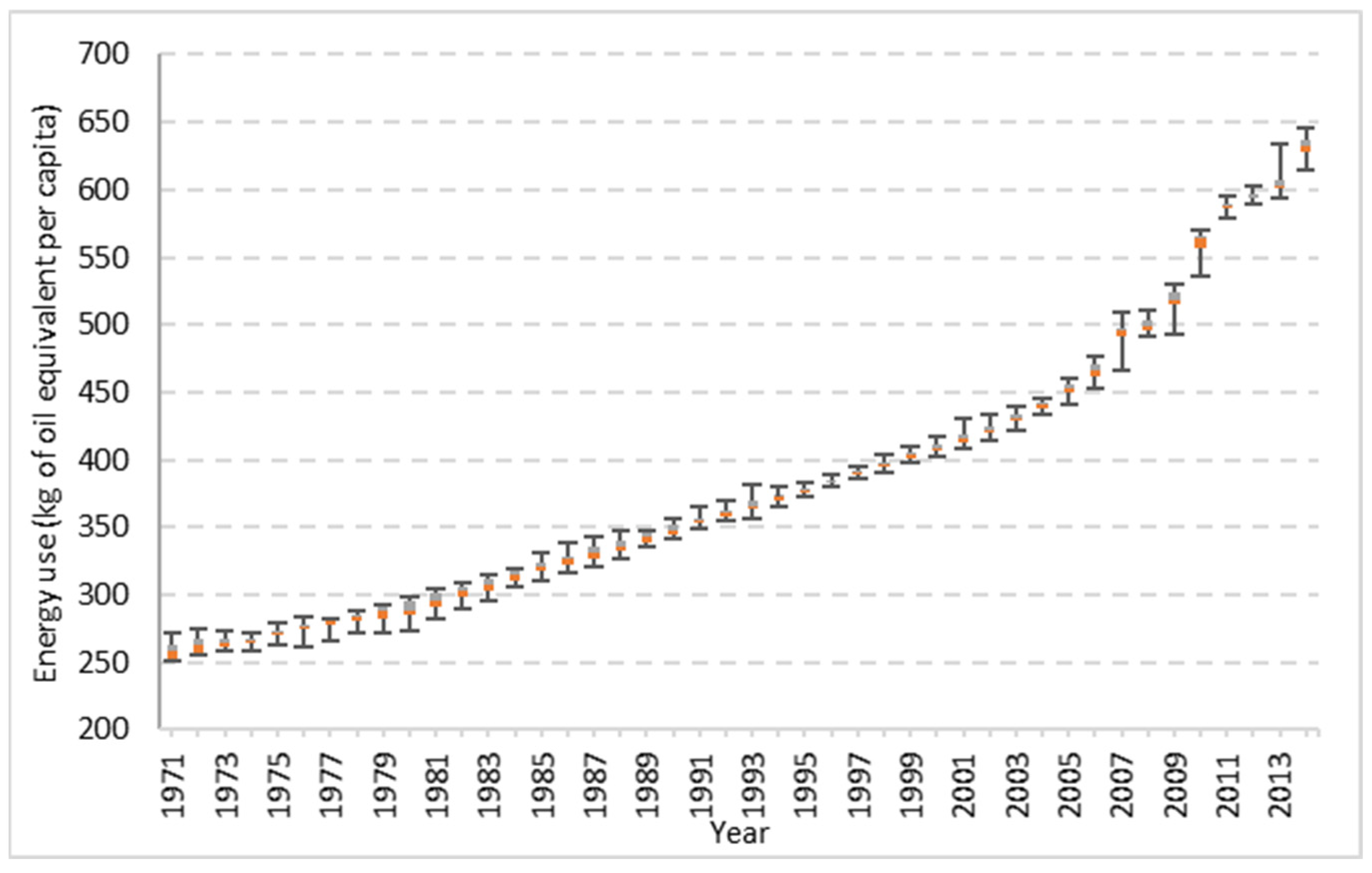
• Analyse long-term historical data of India’s energy use for the period (1971–2014).
• Quantify the performance of ensemble of algorithms (GE-DE) to the energy-use estimation and prediction problems.
• Analyse the associated uncertainties produced from the models in terms of statistical errors.
• Select the best model using the Global Performance Index (GPI) and compare the average estimations and projections with the one from the best model.
• Project the energy-use behaviour for India until the year 2022.

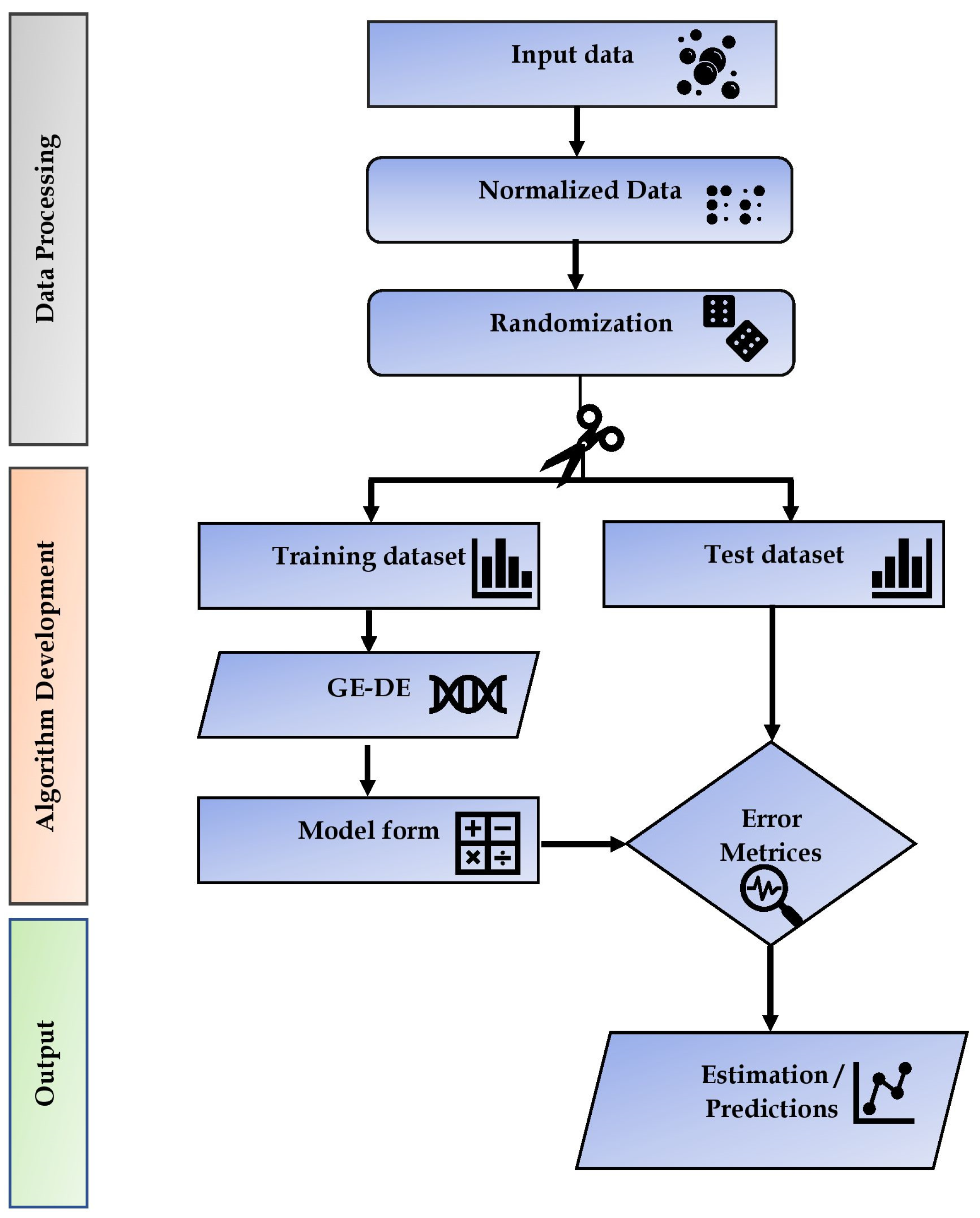
The article is structured into three main sections. Section 2 describes the source, collection, and pre-processing of data; the definition of the problem; and the objective function together with the metrics used to analyse the models. Section 3 presents the results obtained for each of the problems defined and the verification of the results. Finally, Section 4 concludes the work and provides recommendations for future work.

2. Methodology

2.1. Selection of Data

The data for the study of energy use in India have been obtained from the World Bank database [28]. The target (or the output of the model) is the energy use (in kg of oil equivalent per capita). The input data comprise four features which were found to be most influential on the energy use in the modelling approaches presented in the literature: (i) Gross Domestic Product (GDP, in current US$), (ii) population (total), (iii) exports of goods and services (current US$), and (iv) imports of goods and services (current US$). The data, as annual values for all four inputs and the output (energy use), were selected from 1971 to 2014 (44 years) based on availability.

For the sake of simplicity and ease, we denote energy use (in kg of oil equivalent per capita) as E, Gross Domestic Product (GDP in current US$) as X1, population (total) as X2, exports of goods and services (current US$) as X3, and imports of goods and services (current US$) as X4.

Table 2. Correlation matrix for the historical data of energy and the selected socio-economic parameters.

	Energy Use (E)	GDP (X1)	Population (X2)	Exports (X3)	Imports (X4)
Energy use (E)	1.0000	0.9655	0.9515	0.9354	0.9268
GDP (X1)	0.9655	1.0000	0.8596	0.9925	0.9893
Population (X2)	0.9515	0.8596	1.0000	0.8061	0.7961
Exports (X3)	0.9354	0.9925	0.8061	1.0000	0.9978
Imports (X4)	0.9268	0.9893	0.7961	0.9978	1.0000

shows the correlation matrix based on the data obtained. It can be seen that ‘Energy Use’ (E) has a strong correlation with the selected socio-economic parameters, with the highest correlation with GDP of 0.9655, followed by population with a correlation of 0.9515, exports of goods and services with a correlation of 0.9354, and finally, imports of goods and services with a correlation of 0.9268. The results confirm that the selected socio-economic parameters influence the energy-use behaviour of the country and were appropriately selected for the modelling procedure.

2.2. Selection of Training and Test Datasets

Data for the target value and input parameters had different ranges which can affect optimization. Thus, before the data were fed to the algorithm, a normalization process was applied to the data, which was performed by dividing all the values of a parameter by the corresponding maximum value as:

$$E_{i,n}=\frac{E_i}{E_{max}} \mathrm{a}\mathrm{n}\mathrm{d} X_{i,n}=\frac{X_{i,j}}{X_{i,max}}$$

(1)

Consequently, the normalized target values (${\mathrm{E}}_{\mathrm{i},\mathrm{n}}$) and each of the inputs (${\mathrm{X}}_{1\mathrm{n}},{\mathrm{X}}_{2\mathrm{n}},{\mathrm{X}}_{3\mathrm{n}} \mathrm{a}\mathrm{n}\mathrm{d} {\mathrm{X}}_{4\mathrm{n}}$) were normalized with a maximum value of one.

An outline of the methodology followed under the current work is presented in Figure 1.

Following this, the complete data were bifurcated into training and test datasets. The training dataset was used to train the algorithm, while the test dataset was used to test the algorithm’s accuracy on the independent dataset. The process of bifurcation was purely random. In any case (estimation or prediction), half of the data were reserved for training and the rest for the test. More details on the problem formulations and the functioning of algorithms will be presented in the coming sections.

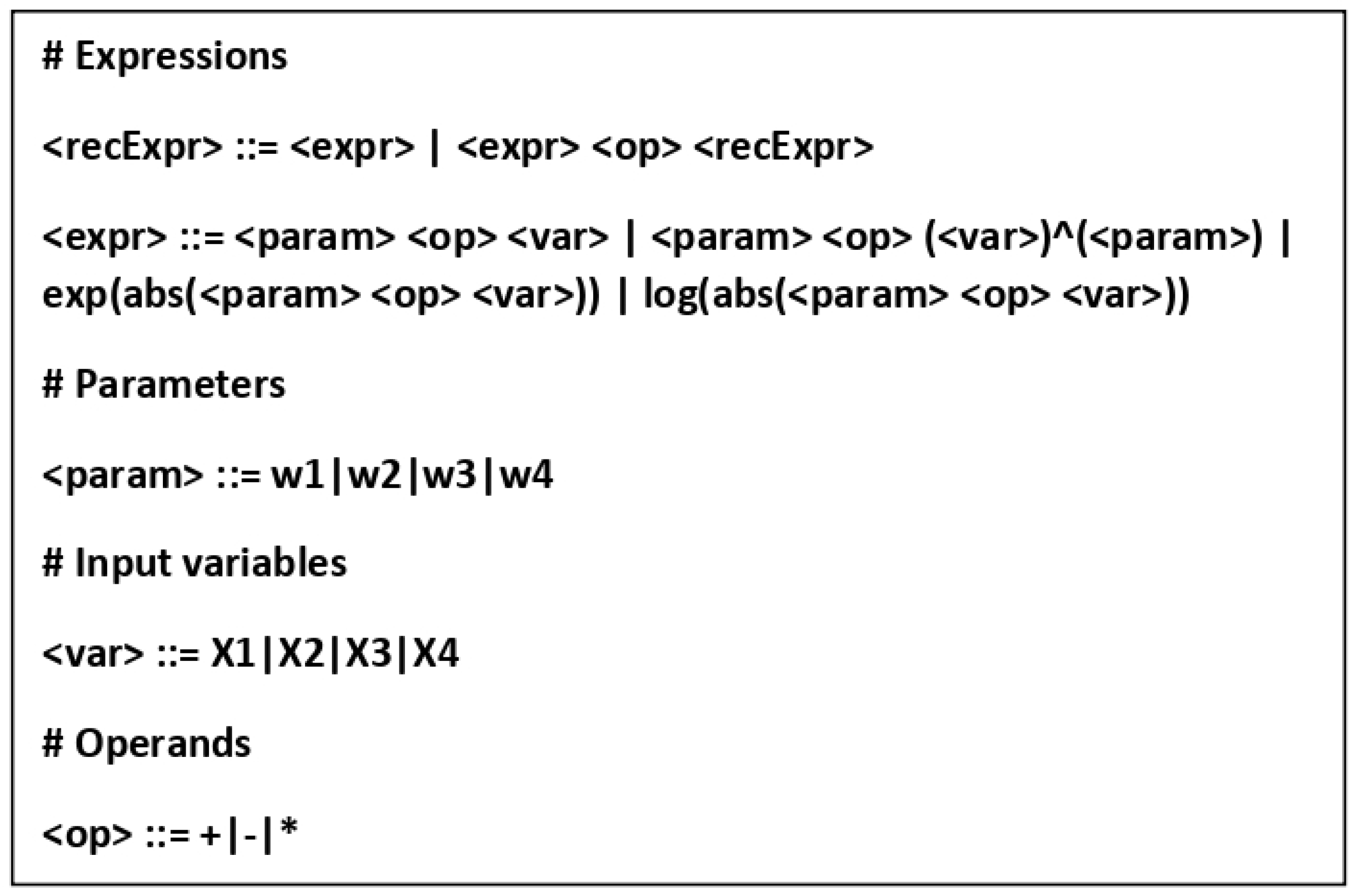
2.3. Problem Definition

Under the present work, two approaches are presented for quantifying energy-use behaviour in India, viz, estimation and prediction. These are explained below.

This study refers to the estimation problem of the target value and the input variables from the same year. The energy-use estimation problem is considered an optimization problem, and the general definition in mathematical form can be defined as:

$$E_{i,t}=f{\left(X_{ji}\right)}_t$$

(2)

where $E_{i,t}$ defines the energy use, with $i=1,2\dots n$, n being the number of data points in the complete dataset; $j$ refers to the input variables $(j=1,2,3,4)$; and suffix $t$ describes that both the sides of equation denote the same year. In other words, the estimation problems require estimating energy use from the input parameters from the same year.

On the other hand, a prediction problem is also considered an optimization problem. However, here, the energy use for a year-ahead $\left(E_{t+1}\right)$ was predicted from the inputs of the current year. Mathematically,

$$E_{i,t+1}=f{\left(X_{ji}\right)}_t$$

(3)

Thus, for each of the above-defined problems, the combination of metaheuristic algorithms (GE-DE) were applied to optimize the target value. The algorithms are explained in the following Section 2.4.

2.4. Algorithmic Methods

Under the current approach, an ensemble of Grammatical Evolution (GE) and Differential Evolution (DE) has been applied to both optimization problems of energy use, as presented in the previous section.

Grammatical Evolution (GE) is an Evolutionary Algorithm (EA) belonging to the class of Genetic Programming (GP) that was introduced by O’Neill and Ryan [29] and utilizes the Backus–Naur Form (BNF) grammar definition for generating a variable-length binary string. GE depends on the process of automatic programming while incorporating unique ways of using grammar. GE uses variable-length binary string genomes to degenerate the genetic code, where each codon represents an integer value, and every codon is a group of 8-bits. Based on the BNF definition, these integer values are then used to create appropriate production rules for the mapping process.

Differential Evolution (DE) is an optimization algorithm that belongs to the Evolutionary Algorithms class. Although known for its simplicity, DE is considered one of the most powerful tools for global optimization. Within the optimization algorithms, DE is a population-based optimizer. It is observed to have the advantages of attaining global optimum combined with excellent precision, fast convergence, self-adaptation, and zero-order information about the objective function.

To summarize, the advantage of using GE is its ability to guide the search of an algorithm using grammar. Meanwhile, DE represents a metaheuristic algorithm better suited for problems where some parameter values need to be found [10].

Figure 2 provides the flowchart of the schema for the execution of GE-DE, while Figure 3 provides the recursive grammar driven by GE together with DE used in the present study.

The GE algorithm develops an expression (a form of a model) using the input variables (X1, X2, X3, and X4) represented as <var> using the functions provided under the <expr>, and these can result in linear, power, exponential and logarithmic. The <recExpr> combines the <expr> with another expression developed in a recursive fashion using the operands denoted by <op>, which can be an addition, subtraction, or multiplication. DE optimizes the coefficients of the variables denoted by w_i for each of the expressions in the recursive expression.

The properties of the algorithmic methods are shown in

Table 3. Properties of the experiments.

Properties of GE
Generations	50
Crossover Probability	0.65
Population	20
Mutation Probability	0.1
Max Wraps	3
Number of Codons	100
Tournament	2
Number of Runs	20
Properties of DE
Recombination Factor:	0.88
Mutation Factor	0.47
Population Size	20

for GE and DE, respectively.

As observed from Table 2, since the “number of runs” was set to 20, we obtained an average of 20 models from the algorithms. However, in the following section, we will look at each run individually and try to analyse and assess the models’ performance in terms of their structure and statistical errors.

2.5. Objective Function and Error Analysis

The accuracy of estimation and predictions was analysed in terms of the root mean squared error (RMSE), as shown in Equation (4), which was used as the objective function.

$$RMSE=\sqrt{\frac{1}{n}{\sum }_{i=1}^n{\left(E_{est,i}-E_{act,i}\right)}^2}$$

(4)

$E_{act,i}$ and $E_{est,i}$ in Equation (4) are the actual and estimated (or predicted) values of energy use.

While other statistics in Equations (5)–(8), viz, average error (AE), coefficient of determination (R²), absolute error (ABS), and relative error (RE), are also used to evaluate the accuracy as follows:

$$AE=\frac{1}{n}{\sum }_{i=1}^n(E_{est,i}-E_{act,i})$$

(5)

$$R^2=\frac{{\sum }_{i=1}^n(E_{est,i}-E_{est,avg})(E_{act,i}-E_{act,avg})}{\sqrt{{\sum }_{i=1}^n{(E_{est,i}-E_{est,avg})}^2{\sum }_{i=1}^n{\left(E_{act,i}-E_{act,avg}\right)}^2}}$$

(6)

$$BS=\frac{1}{n}{\sum }_{i=1}^n\left|E_{est,i}-E_{act,i}\right|$$

(7)

$$RE=\frac{1}{n}{\sum }_{i=1}^n\frac{\left|E_{est,i}-E_{act,i}\right|}{E_{act,i}}$$

(8)

These statistics were calculated to ease the comparison between the results obtained in this article and were selected based on previous studies.

2.6. GPI and Ranks of the Models

The literature shows that different evaluation criteria can lead to different outcomes while selecting the most appropriate model. Although the objective function for the algorithm was described as RMSE in the previous section, other metrics also help define the models’ fitness. The Global Performance Index (GPI) is a statistical tool proposed by Despotovic et al. [30]. GPI is a combined metric that uses the equal weights of all the statistical errors that are used.

GPI is calculated from the normalized values (between 0 and 1) of each statistical indicator for all the models (${\tilde{Y}}_{ij}$). For each column of normalized values, a median value is obtained as $\left({\tilde{Y}}_j\right)$. The difference $\left({\tilde{Y}}_j-{\tilde{Y}}_{ij}\right)$ is then calculated. In the final step, a weight factor, ${\alpha }_j$, is multiplied by the obtained difference, and all the values obtained for each model are summed to calculate GPI. Mathematically, GPI is described as (for $i^{th}$ model):

$${GPI}_i={\sum }_{j=1}^n{\alpha }_j\left({\tilde{Y}}_j-{\tilde{Y}}_{ij}\right)$$

(9)

The weight factor ${\alpha }_j=\left\{\begin{array}{c}1 \mathrm{for} RMSE, AE, ABS, RE\\ -1 \mathrm{for} R^2\end{array}\right.$.

3. Results and Discussion

In this section, we look at the models generated from the ensemble of algorithms and the model forms together with outputs (estimated and predicted values) in terms of the statistical errors. Also, we will look at the evolution in the estimated and predicted values of energy-use behaviour as averages and variability from the generated models.

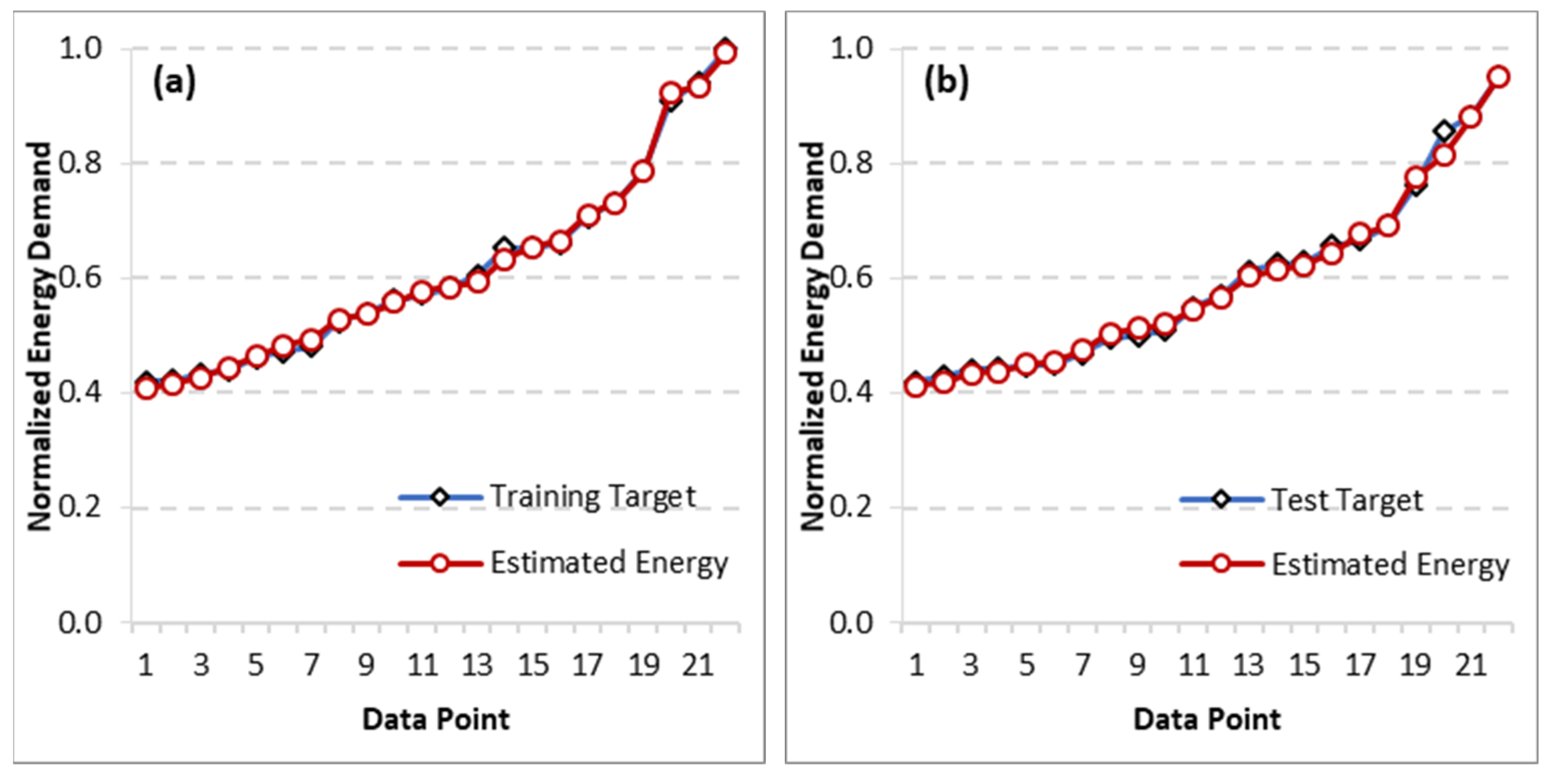
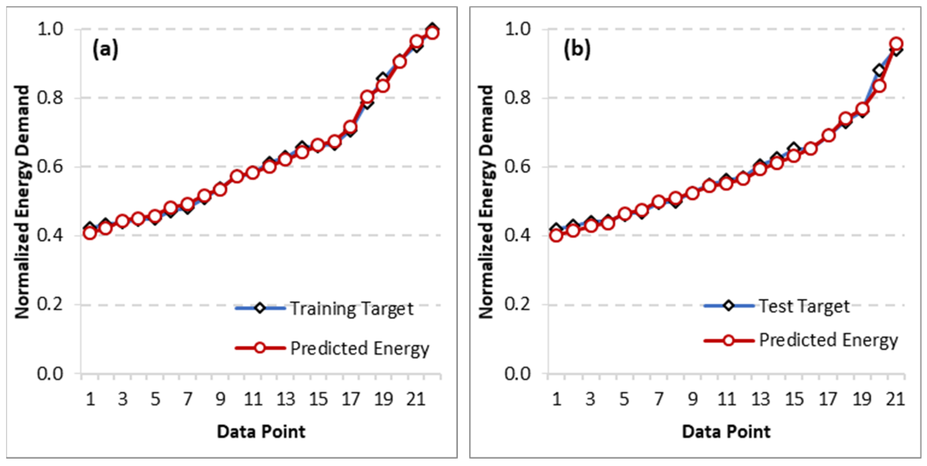
3.1. Estimation Results

The following models (E1–E20) were obtained for the estimation of energy use from the GE-DE algorithms:

$$\mathrm{E}1. {\left(\frac{E_i}{E_{max}}\right)}_t={\left.\left[0.7293{\left(\frac{{X2}_i}{{X2}_{max}}\right)}^{0.7374}\right]-\left[-0.2675{\left(\frac{{X1}_i}{{X1}_{max}}\right)}^{1.9471}\right]\right|}_t$$

(10)

$$\mathrm{E}2. {\left(\frac{E_i}{E_{max}}\right)}_t={\left.\left[0.2777{\left(\frac{{X1}_i}{{X1}_{max}}\right)}^{1.8850}\right]+\left[log\left|1.0481+\left(\frac{{X2}_i}{{X2}_{max}}\right)\right|\right]\right|}_t$$

(11)

$$\begin{gathered} \mathrm{E}3. {\left(\frac{E_i}{E_{max}}\right)}_t={\left.\left[log\left|1.1844+\left(\frac{{X3}_i}{{X3}_{max}}\right)\right|\right]\times \left[1.1844{\left(\frac{{X3}_i}{{X3}_{max}}\right)}^{0.9579}\right]-\left[0.9948\left(\frac{{X2}_i}{{X2}_{max}}\right)\right]-\left[0.9579+ \\ {\left(\frac{{X3}_i}{{X3}_{max}}\right)}^{1.1844}\right]-\left[ln\left|0.9579+\left(\frac{{X3}_i}{{X3}_{max}}\right)\right|\right]\times \left[e^{\left|0.9948-\left(\frac{{X2}_i}{{X2}_{max}}\right)\right|}\right]+\left[e^{\left|0.9948\left(\frac{{X2}_i}{{X2}_{max}}\right)\right|}\right]\right|}_t \end{gathered}$$

(12)

$$\mathrm{E}4. {\left(\frac{E_i}{E_{max}}\right)}_t={\left.\left[0.5929{\left(\frac{{X1}_i}{{X1}_{max}}\right)}^{-0.1710}\right]-\left[-0.5203\left(\frac{{X1}_i}{{X1}_{max}}\right)\right]+\left[0.8683-{\left(\frac{{X2}_i}{{X2}_{max}}\right)}^{-0.5203}\right]\right|}_t$$

(13)

$$\mathrm{E}5. {\left(\frac{E_i}{E_{max}}\right)}_t={\left.\left[\ln \left|\left(0.2257+\left(\frac{{X2}_i}{{X2}_{max}}\right)\right)\right|\right]\times \left[\exp \left|-0.01457+\left(\frac{{X3}_i}{{X3}_{max}}\right)\right|\right]+\left[-0.5331+{\left(\frac{{X1}_i}{{X1}_{max}}\right)}^{-0.0899}\right]\right|}_t$$

(14)

$$\mathrm{E}6. {\left(\frac{E_i}{E_{max}}\right)}_t={\left.\left[0.2777{\left(\frac{{X1}_i}{{X1}_{max}}\right)}^{1.8549}\right]+\left[ln\left|-1.0482-\left(\frac{{X2}_i}{{X2}_{max}}\right)\right|\right]\right|}_t$$

(15)

$$\mathrm{E}7. {\left(\frac{E_i}{E_{max}}\right)}_t={\left.\left[0.3621{\left(\frac{{X1}_i}{{X1}_{max}}\right)}^{0.9576}\right]+\left[0.6099{\left(\frac{{X2}_i}{{X2}_{max}}\right)}^{0.5557}\right]\right|}_t$$

(16)

$$\begin{array}{l}\mathrm{E}8. {\left(\frac{E_i}{E_{max}}\right)}_t=\left[-0.2806{\left(\frac{{X3}_i}{{X3}_{max}}\right)}^{0.4425}\right]\times \left[e^{\left|-1.2387+\left(\frac{{X3}_i}{{X3}_{max}}\right)\right|}\right]-\left[0.0457{\left(\frac{{X1}_i}{{X1}_{max}}\right)}^{0.0457}\right]+\left[e^{\left|-1.2387*\left(\frac{{X2}_i}{{X2}_{max}}\right)\right|}\right]-\\ {\left.\left[e^{\left|-0.2806+\left(\frac{{X2}_i}{{X2}_{max}}\right)\right|}\right]\right|}_t\end{array}$$

(17)

$$\begin{array}{l}\mathrm{E}9. {\left(\frac{E_i}{E_{max}}\right)}_t=\left[ln\left|-0.6785-\left(\frac{{X2}_i}{{X2}_{max}}\right)\right|\right]\times \left[-0.6785-\left(\frac{{X1}_i}{{X1}_{max}}\right)\right]\times \left[-0.1093-{\left(\frac{{X4}_i}{{X4}_{max}}\right)}^{1.3213}\right]\times \\ \left[-0.1093{\left(\frac{{X3}_i}{{X3}_{max}}\right)}^{1.3213}\right]-{\left.\left[-0.1093+{\left(\frac{{X2}_i}{{X2}_{max}}\right)}^{1.2032}\right]\right|}_t\end{array}$$

(18)

$$\begin{array}{l}\mathrm{E}10. {\left(\frac{E_i}{E_{max}}\right)}_t=\left[0.8728{\left(\frac{{X1}_i}{{X1}_{max}}\right)}^{0.8239}\right]\times \left[0.6716{\left(\frac{{X2}_i}{{X2}_{max}}\right)}^{0.8728}\right]+\left[0.6716{\left(\frac{{X1}_i}{{X1}_{max}}\right)}^{-0.2737}\right]\times \\ {\left.\left[ln\left|0.8239+\left(\frac{{X2}_i}{{X2}_{max}}\right)\right|\right]\right|}_t\end{array}$$

(19)

$$\mathrm{E}11. {\left(\frac{E_i}{E_{max}}\right)}_t={\left.\left[0.8409\left(\frac{{X2}_i}{{X2}_{max}}\right)\right]+\left[e^{\left|0.4634\left(\frac{{X1}_i}{{X1}_{max}}\right)\right|}\right]\times \left[0.7251-{\left(\frac{{X1}_i}{{X1}_{max}}\right)}^{0.1138}\right]\right|}_t$$

(20)

$$\mathrm{E}12. {\left(\frac{E_i}{E_{max}}\right)}_t={\left.\left[-0.7569+{\left(\frac{{X3}_i}{{X3}_{max}}\right)}^{-0.0612}\right]\times \left[e^{\left|0.3669\left(\frac{{X1}_i}{{X1}_{max}}\right)\right|}\right]+\left[ln\left|0.3669+\left(\frac{{X2}_i}{{X2}_{max}}\right)\right|\right]\right|}_t$$

(21)

$$\mathrm{E}13. {\left(\frac{E_i}{E_{max}}\right)}_t={\left.\left[-0.1933+\left(\frac{{X2}_i}{{X2}_{max}}\right)\right]\times \left[1.3763\left(\frac{{X1}_i}{{X1}_{max}}\right)\right]\times \left[0.2294\left(\frac{{X2}_i}{{X2}_{max}}\right)\right]+\left[ln\left|1.3763+\left(\frac{{X2}_i}{{X2}_{max}}\right)\right|\right]\right|}_t$$

(22)

$$\mathrm{E}14. {\left(\frac{E_i}{E_{max}}\right)}_t={\left.\left[ln\left|-0.01908-\left(\frac{{X1}_i}{{X1}_{max}}\right)\right|\right]\times \left[-0.2832{\left(\frac{{X1}_i}{{X1}_{max}}\right)}^{1.0606}\right]\times \left[-1.9291+\left(\frac{{X2}_i}{{X2}_{max}}\right)\right]\right|}_t$$

(23)

$$\begin{array}{l}\mathrm{E}15. {\left(\frac{E_i}{E_{max}}\right)}_t=\left[1.1203{\left(\frac{{X1}_i}{{X1}_{max}}\right)}^{-0.0660}\right]-\left[-0.2447\left(\frac{{X3}_i}{{X3}_{max}}\right)\right]\times \left[e^{\left|-0.4696\left(\frac{{X1}_i}{{X1}_{max}}\right)\right|}\right]-\\ {\left.\left[-0.4696{\left(\frac{{X2}_i}{{X2}_{max}}\right)}^{-0.4696}\right]\right|}_t\end{array}$$

(24)

$$\begin{array}{l}\mathrm{E}16. {\left(\frac{E_i}{E_{max}}\right)}_t=\left[0.3573{\left(\frac{{X1}_i}{{X1}_{max}}\right)}^{2.1556}\right]-\left[0.3573-\left(\frac{{X3}_i}{{X3}_{max}}\right)\right]+\left[0.3573+{\left(\frac{{X3}_i}{{X3}_{max}}\right)}^{0.8374}\right]+\\ {\left.\left[-0.3551+{\left(\frac{{X2}_i}{{X2}_{max}}\right)}^{0.3573}\right]\right|}_t\end{array}$$

(25)

$$\mathrm{E}17. {\left(\frac{E_i}{E_{max}}\right)}_t={\left.\left[0.2651{\left(\frac{{X1}_i}{{X1}_{max}}\right)}^{2.0093}\right]+\left[0.7321{\left(\frac{{X2}_i}{{X2}_{max}}\right)}^{0.7432}\right]\right|}_t$$

(26)

$$\mathrm{E}18. {\left(\frac{E_i}{E_{max}}\right)}_t={\left.\left[0.5062+{\left(\frac{{X1}_i}{{X1}_{max}}\right)}^{0.5681}\right]\times \left[-0.9627+\left(\frac{{X1}_i}{{X1}_{max}}\right)\right]+\left[ln\left|0.5681+\left(\frac{{X2}_i}{{X2}_{max}}\right)\right|\right]\right|}_t$$

(27)

$$\mathrm{E}19. {\left(\frac{E_i}{E_{max}}\right)}_t={\left.\left[1.6171-{\left(\frac{{X2}_i}{{X2}_{max}}\right)}^{-0.2474}\right]+\left[0.6058\left(\frac{{X2}_i}{{X2}_{max}}\right)\right]\times \left[0.6058\left(\frac{{X1}_i}{{X1}_{max}}\right)\right]\right|}_t$$

(28)

$$\begin{array}{l}\mathrm{E}20. {\left(\frac{E_i}{E_{max}}\right)}_t=\left[0.3809+{\left(\frac{{X2}_i}{{X2}_{max}}\right)}^{0.3809}\right]\times \left[e^{\left|0.3809\left(\frac{{X1}_i}{{X1}_{max}}\right)\right|}\right]-\left[0.0700{\left(\frac{{X3}_i}{{X3}_{max}}\right)}^{0.3809}\right]+\left[0.2604\left(\frac{{X2}_i}{{X2}_{max}}\right)\right]-\\ {\left.\left[0.07004+{\left(\frac{{X2}_i}{{X2}_{max}}\right)}^{0.38094}\right]\times \left[0.04804-{\left(\frac{{X3}_i}{{X3}_{max}}\right)}^{0.04804}\right]\right|}_t\end{array}$$

(29)

The number of terms (in parenthesis) in an equation is between two and seven, as represented within the brackets. Further, the number of times an input parameter appears in the 20 runs or models generated from the algorithm (Equations (10)–(29)) is depicted in Figure 4. X2 (population, total) appears as the maximum number of 30 times in the models, followed by X1 (GDP) with 25, X3 (number of exports) with 14, and, finally, the least of X4 (number of imports) with one. Thus, the most crucial parameter that affects energy use is population.

Table 4. Statistical errors obtained based on estimation accuracy of the training and test dataset.

	Training Dataset					Test Dataset
Model	RMSE	Av. Error	R2	Ab. Error	Rel. Error	RMSE	Av. Error	R2	Ab. Error	Rel. Error
E1	0.0108	0.0086	0.9959	0.1899	0.0161	0.0135	0.0107	0.9925	0.2361	0.0189
E2	0.0111	0.0090	0.9956	0.1988	0.0167	0.0138	0.0110	0.9922	0.2429	0.0194
E3	0.0085	0.0062	0.9974	0.1371	0.0103	0.0160	0.0104	0.9896	0.2294	0.0151
E4	0.0108	0.0090	0.9975	0.1981	0.0153	0.0143	0.0112	0.9950	0.2461	0.0193
E5	0.0112	0.0097	0.9958	0.2129	0.0160	0.0231	0.0135	0.9792	0.2971	0.0193
E6	0.0111	0.0090	0.9956	0.1988	0.0167	0.0138	0.0110	0.9922	0.2429	0.0194
E7	0.0154	0.0143	0.9917	0.3141	0.0240	0.0160	0.0139	0.9892	0.3058	0.0237
E8	0.0115	0.0092	0.9960	0.2019	0.0155	0.0190	0.0151	0.9875	0.3330	0.0256
E9	0.0121	0.0094	0.9948	0.2079	0.0151	0.0132	0.0102	0.9934	0.2233	0.0164
E10	0.0078	0.0060	0.9979	0.1328	0.0099	0.0103	0.0069	0.9958	0.1515	0.0108
E11	0.0081	0.0071	0.9977	0.1552	0.0117	0.0110	0.0074	0.9951	0.1632	0.0116
E12	0.0097	0.0076	0.9967	0.1666	0.0135	0.0170	0.0136	0.9879	0.3000	0.0251
E13	0.0115	0.0100	0.9953	0.2208	0.0171	0.0128	0.0109	0.9931	0.2395	0.0185
E14	0.0117	0.0098	0.9957	0.2159	0.0170	0.0137	0.0082	0.9930	0.1798	0.0141
E15	0.0127	0.0098	0.9943	0.2158	0.0165	0.0176	0.0110	0.9889	0.2412	0.0171
E16	0.0118	0.0098	0.9951	0.2167	0.0179	0.0143	0.0122	0.9916	0.2693	0.0208
E17	0.0108	0.0086	0.9959	0.1894	0.0161	0.0136	0.0106	0.9924	0.2341	0.0187
E18	0.0080	0.0061	0.9977	0.1349	0.0105	0.0109	0.0074	0.9954	0.1623	0.0118
E19	0.0141	0.0128	0.9929	0.2824	0.0226	0.0154	0.0133	0.9900	0.2922	0.0233
E20	0.0102	0.0079	0.9965	0.1739	0.0134	0.0139	0.0116	0.9918	0.2553	0.0204

provides the comparison of values of statistical errors for training as well as the test dataset.

From the table, it can be observed that the values of computed statistical errors are small, and this represents a high estimation accuracy. On the training dataset, the RMSE ranges from 0.0078 for Model E10 to 0.0154 for Model E7. However, other models, e.g., E18 with an RMSE of 0.0080 and Model E11 with an RMSE of 0.0081, also represent very accurate estimations. Analysing the form of Model E10 (Equation (19)), it is observed that the equation has four terms in total, with two terms each containing X1 and X2. Since X2 and X1 appear the highest number of times overall in the equations (as previously discussed in Figure 3), it is justified that the dependence of a model towards X1 and X2 represents better estimation accuracy.

Further, each of the other statistical errors has a value that indicates the accuracy of Model E10, whose errors are the lowest compared to the rest of the obtained models (average error 0.0060, R² 0.9979, absolute error 0.1328, and relative error 0.0099). On the testing dataset, the best-resulting equation for statistical errors is again Model E10, with RMSE of 0.0103, average error of 0.0069, R² of 0.9958, absolute error of 0.1515, and relative error of 0.0108). Like the training dataset, E18 and E11 also have comparable RMSE values of 0.0109 and 0.0110, respectively, compared to E10.

Figure 5a,b show the algorithm’s performance for estimation on the training and test datasets, respectively, representing the normalized energy data points. The deviation of estimated energy from the data points is visibly slight, with the estimated data points following the actual data very closely.

The energy use (in kgoe/capita) was computed back from the normalized value, and the evolution of energy use is represented (1971–2014) in Figure 6 as a box-and-whiskers chart to provide the variability from all 20 models (as Section 3.1 describes). Thus, for any year in the chart, the middle line represents the median energy-use value, the box’s ends represent the first and third quartiles, and the end of the whiskers represents the minimum and maximum values.

The error computation for the estimated energy use was performed for the 20 runs (or models) obtained from the experiment and is presented in

Table 5. Statistical errors obtained for the 20 estimation models and the average estimation for estimated energy use.

Model	RMSE	Average Error	R2	Absolute Error	Relative Error
E1	7.7848	0.2791	0.9943	6.1628	0.0175
E2	7.9891	−0.1134	0.9940	6.3903	0.0180
E3	8.1561	−1.0204	0.9938	5.3027	0.0127
E4	8.0769	−5.1273	0.9963	6.4256	0.0173
E5	11.5509	−1.7066	0.9876	7.3791	0.0176
E6	7.9894	−0.0920	0.9940	6.3912	0.0180
E7	9.9752	−0.5650	0.9906	8.9674	0.0239
E8	9.9787	−3.9315	0.9920	7.7387	0.0205
E9	8.0673	−1.0981	0.9941	6.2383	0.0157
E10	5.8183	−0.7111	0.9969	4.1126	0.0103
E11	6.1505	−0.5451	0.9965	4.6057	0.0116
E12	8.8273	−0.1168	0.9927	6.7507	0.0193
E13	7.7427	0.3319	0.9943	6.6594	0.0178
E14	8.1162	−1.7528	0.9942	5.7251	0.0156
E15	9.7573	−1.7161	0.9914	6.6119	0.0168
E16	8.3510	0.1795	0.9934	7.0310	0.0193
E17	7.8158	0.1059	0.9943	6.1266	0.0174
E18	6.0823	−0.9723	0.9966	4.2995	0.0111
E19	9.4171	0.2882	0.9916	8.3122	0.0229
E20	7.7695	0.2433	0.9944	6.2092	0.0169
Average	6.3749	−0.9020	0.9962	4.6263	0.0125

.

The average RMSE is 6.3749 kgoe/capita, representing a very accurate energy-use estimation. Among the models, the most negligible value of RMSE (=5.8183 kgoe/capita) was obtained for model E10, Model 6 has the least value of the average error of −0.0920 kgoe/capita, Model 10 again has the highest R² = 0.9969, and minimum values of absolute error of 4.1126 kgoe/capita and relative error of 0.0103 were found.

Following the calculation of statistical errors for estimated energy use, the procedure for calculating the GPI and, correspondingly, creating a ranking of the models was applied (as previously discussed in Section 2.6). The values of GPI and the ranking of the models are represented in

Table 6. GPI and ranks of the estimation models.

S. No.	Model	GPI	Rank
1	E1	−0.0307	10
2	E2	−0.1143	11
3	E3	0.6171	5
4	E4	1.0844	4
5	E5	−1.3052	18
6	E6	−0.1186	12
7	E7	−1.7070	20
8	E8	−0.4355	15
9	E9	0.2598	7
10	E10	1.7249	1
11	E11	1.3906	3
12	E12	−0.5750	17
13	E13	−0.1576	13
14	E14	0.5077	6
15	E15	−0.3665	14
16	E16	−0.5197	16
17	E17	0.0038	9
18	E18	1.5958	2
19	E19	−1.4532	19
20	E20	0.0220	8

.

The GPI values range from −1.7070 for Model 7 to 1.7249 for Model 10. Therefore, the best model for estimating energy use, again, is E10.

Figure 7 compares actual energy use, the estimated energy use from Model 10, and the average estimated value from all 20 models.

3.2. Prediction Results

We now look at the prediction of energy use, where the energy use for the next year is predicted using the input variables from the current year. The following models (P1–P20) were obtained to predict energy use.

$$\begin{gathered} {\left(\frac{E_i}{E_{max}}\right)}_{t+1}={\left.\left[0.6899{\left(\frac{{X1}_i}{{X1}_{max}}\right)}^{0.4354}\right]-\left[-1.3234{\left(\frac{{X2}_i}{{X2}_{max}}\right)}^{0.4563}\right]-\left[0.4563+\left(\frac{{X3}_i}{{X3}_{max}}\right)\right]\times \left[0.4354- \\ {\left(\frac{{X1}_i}{{X1}_{max}}\right)}^{0.4563}\right]\right|}_t \end{gathered}$$

(30)

$${\left(\frac{E_i}{E_{max}}\right)}_{t+1}={\left.\left[-0.3077+{\left(\frac{{X2}_i}{{X2}_{max}}\right)}^{-0.4626}\right]+\left[e^{\left|-1.0912\left(\frac{{X1}_i}{{X1}_{max}}\right)\right|}\right]\times \left[ln|-1.1111\left(\frac{{X2}_i}{{X2}_{max}}\right)|\right]\right|}_t$$

(31)

$$\begin{gathered} {\left(\frac{E_i}{E_{max}}\right)}_{t+1}={\left.\left[-0.4826{\left(\frac{{X3}_i}{{X3}_{max}}\right)}^{0.3828}\right]+\left[-1.1287\left(\frac{{X1}_i}{{X1}_{max}}\right)\right]\times \left[0.3828{\left(\frac{{X4}_i}{{X4}_{max}}\right)}^{0.3828}\right]-\left[-0.4826+\left(\frac{{X3}_i}{{X3}_{max}}\right)\right]+ \\ \left[ln\left|-0.5375-\left(\frac{{X2}_i}{{X2}_{max}}\right)\right|\right]\right|}_t \end{gathered}$$

(32)

$${\left(\frac{E_i}{E_{max}}\right)}_{t+1}={\left.\left[0.3527\left(\frac{{X3}_i}{{X3}_{max}}\right)\right]+\left[0.0543-{\left(\frac{{X1}_i}{{X1}_{max}}\right)}^{0.0543}\right]-\left[-1.5851{\left(\frac{{X2}_i}{{X2}_{max}}\right)}^{0.3527}\right]\right|}_t$$

(33)

$${\left(\frac{E_i}{E_{max}}\right)}_{t+1}={\left.\left[ln\left|-1.0370-\left(\frac{{X2}_i}{{X2}_{max}}\right)\right|\right]-\left[-0.2681\left(\frac{{X3}_i}{{X3}_{max}}\right)\right]\right|}_t$$

(34)

$${\left(\frac{E_i}{E_{max}}\right)}_{t+1}={\left.\left[0.3709{\left(\frac{{X3}_i}{{X3}_{max}}\right)}^{1.1855}\right]-\left[e^{\left|0.3709\left(\frac{{X1}_i}{{X1}_{max}}\right)\right|}\right]\times \left[0.2611+{\left(\frac{{X2}_i}{{X2}_{max}}\right)}^{0.5105}\right]\right|}_t$$

(35)

$${\left(\frac{E_i}{E_{max}}\right)}_{t+1}={\left.\left[0.1155-\left(\frac{{X4}_i}{{X4}_{max}}\right)\right]+\left[0.1155-{\left(\frac{{X2}_i}{{X2}_{max}}\right)}^{1.2967}\right]\times \left[-0.5011+\left(\frac{{X3}_i}{{X3}_{max}}\right)\right]\times \left[0.2459+\left(\frac{{X4}_i}{{X4}_{max}}\right)\right]\right|}_t$$

(36)

$${\left(\frac{E_i}{E_{max}}\right)}_{t+1}={\left.\left[ln\left|-1.0468-\left(\frac{{X2}_i}{{X2}_{max}}\right)\right|\right]+\left[0.2724{\left(\frac{{X3}_i}{{X3}_{max}}\right)}^{1.1910}\right]\right|}_t$$

(37)

$${\left(\frac{E_i}{E_{max}}\right)}_{t+1}={\left.\left[0.6389{\left(\frac{{X3}_i}{{X3}_{max}}\right)}^{-0.5956}\right]\times \left[0.6389\left(\frac{{X3}_i}{{X3}_{max}}\right)\right]\times \left[\mathit{ln}\left|0.6389+\left(\frac{{X1}_i}{{X1}_{max}}\right)\right|\right]+\left[0.7776{\left(\frac{{X2}_i}{{X2}_{max}}\right)}^{0.7508}\right]\right|}_t$$

(38)

$${\left(\frac{E_i}{E_{max}}\right)}_{t+1}={\left.\left[0.2663{\left(\frac{{X3}_i}{{X3}_{max}}\right)}^{1.223}\right]+\left[0.7231{\left(\frac{{X2}_i}{{X2}_{max}}\right)}^{0.7231}\right]\right|}_t$$

(39)

$${\left(\frac{E_i}{E_{max}}\right)}_{t+1}={\left.\left[e^{\left|-0.2516\left(\frac{{X3}_i}{{X3}_{max}}\right)\right|}\right]-\left[1.2991+{\left(\frac{{X2}_i}{{X2}_{max}}\right)}^{0.4492}\right]\right|}_t$$

(40)

$${\left(\frac{E_i}{E_{max}}\right)}_{t+1}={\left.\left[0.2573{\left(\frac{{X3}_i}{{X3}_{max}}\right)}^{1.2890}\right]-\left[-0.7331{\left(\frac{{X2}_i}{{X2}_{max}}\right)}^{0.7514}\right]\right|}_t$$

(41)

$${\left(\frac{E_i}{E_{max}}\right)}_{t+1}={\left.\left[0.7301{\left(\frac{{X2}_i}{{X2}_{max}}\right)}^{0.7438}\right]+\left[0.2595{\left(\frac{{X3}_i}{{X3}_{max}}\right)}^{1.2786}\right]\right|}_t$$

(42)

$${\left(\frac{E_i}{E_{max}}\right)}_{t+1}={\left.\left[-0.3796{\left(\frac{{X3}_i}{{X3}_{max}}\right)}^{1.0995}\right]\times \left[-0.9078+{\left(\frac{{X1}_i}{{X1}_{max}}\right)}^{-0.0861}\right]\times \left[ln\left|-0.9078-\left(\frac{{X2}_i}{{X2}_{max}}\right)\right|\right]\right|}_t$$

(43)

$$\begin{gathered} {\left(\frac{E_i}{E_{max}}\right)}_{t+1}={\left.\left[0.0937+{\left(\frac{{X1}_i}{{X1}_{max}}\right)}^{0.7299}\right]\times \left[ln\left|0.1566+\left(\frac{{X4}_i}{{X4}_{max}}\right)\right|\right]\times \left[0.0937+\left(\frac{{X2}_i}{{X2}_{max}}\right)\right]\times \left[0.7299+\left(\frac{{X1}_i}{{X1}_{max}}\right)\right]\times \\ \left[0.1599\left(\frac{{X3}_i}{{X3}_{max}}\right)\right]\right|}_t \end{gathered}$$

(44)

$$\begin{gathered} {\left(\frac{E_i}{E_{max}}\right)}_{t+1}={\left.\left[0.1645{\left(\frac{{X1}_i}{{X1}_{max}}\right)}^{1.0933}\right]-\left[e^{\left|0.1645-\left(\frac{{X1}_i}{{X1}_{max}}\right)\right|}\right]\times \left[0.0412\left(\frac{{X3}_i}{{X3}_{max}}\right)\right]-\left[0.1645{\left(\frac{{X4}_i}{{X4}_{max}}\right)}^{0.3397}\right]+ \\ \left[0.3397\left(\frac{{X3}_i}{{X3}_{max}}\right)\right]+\left[ln\left|1.0933+\left(\frac{{X2}_i}{{X2}_{max}}\right)\right|\right]\right|}_t \end{gathered}$$

(45)

$${\left(\frac{E_i}{E_{max}}\right)}_{t+1}={\left.\left[0.2724{\left(\frac{{X3}_i}{{X3}_{max}}\right)}^{1.1928}\right]+\left[ln\left|(1.0470+\left(\frac{{X2}_i}{{X2}_{max}}\right)\right|\right]\right|}_t$$

(46)

$${\left(\frac{E_i}{E_{max}}\right)}_{t+1}={\left.\left[0.7310{\left(\frac{{X2}_i}{{X2}_{max}}\right)}^{0.7438}\right]-\left[-0.2603{\left(\frac{{X3}_i}{{X3}_{max}}\right)}^{1.2887}\right]\right|}_t$$

(47)

$${\left(\frac{E_i}{E_{max}}\right)}_{t+1}={\left.\left[0.2667{\left(\frac{{X1}_i}{{X1}_{max}}\right)}^{1.5734}\right]+\left[ln\left|1.0393+\left(\frac{{X2}_i}{{X2}_{max}}\right)\right|\right]\right|}_t$$

(48)

$$\begin{gathered} {\left(\frac{E_i}{E_{max}}\right)}_{t+1}={\left.\left[0.8826{\left(\frac{{X3}_i}{{X3}_{max}}\right)}^{0.9528}\right]+\left[0.8826{\left(\frac{{X2}_i}{{X2}_{max}}\right)}^{-0.2309}\right]-\left[ln\left|-1.0503-\left(\frac{{X3}_i}{{X3}_{max}}\right)\right|\right]+ \\ \left[-1.0503+\left(\frac{{X2}_i}{{X2}_{max}}\right)\right]\right|}_t \end{gathered}$$

(49)

We analysed the structure of the models in terms of the number of terms that appear in the equation and the number of times an input variable appears in total in all the models. The number of terms varies from two to six in the prediction models, with most of the models consisting of only two terms. Further, as depicted in Figure 8, X2 and X3 appear an equal number of times (i.e., 22) in the model equations, followed by X1 13 times and X4 five times. Therefore, compared to the estimation results (Section 3.2), the input parameters of population (X2) and exports (X3) show a higher effect in the case of prediction models. This difference in the outcomes can be attributed to the fact that the data fed to the algorithm are organised differently, as discussed in the problem statements, i.e., the prediction problem requires the input data from the current year to be used to predict the energy use for the next year, which is the fundamental explanation of the “year-ahead” energy prediction, while in the case of estimation problem, the input and the target value both belong to the same year.

Statistical errors were calculated for the prediction models and are tabulated in

Table 7. Statistical errors obtained based on prediction accuracy of the training and test datasets.

	Training Dataset					Testing Dataset
Model	RMSE	Avg. Error	R2	Ab. Error	Rel. Error	RMSE	Avg. Error	R2	Ab. Error	Rel. Error
P1	0.0098	0.0090	0.9969	0.1984	0.0150	0.0159	0.0108	0.9890	0.2260	0.0172
P2	0.0159	0.0112	0.9920	0.2466	0.0169	0.0123	0.0077	0.9932	0.1613	0.0122
P3	0.0099	0.0082	0.9967	0.1801	0.0137	0.0188	0.0118	0.9849	0.2469	0.0194
P4	0.0096	0.0082	0.9970	0.1801	0.0132	0.0147	0.0101	0.9909	0.2115	0.0156
P5	0.0120	0.0093	0.9952	0.2055	0.0154	0.0151	0.0121	0.9906	0.2536	0.0208
P6	0.0104	0.0091	0.9964	0.2012	0.0156	0.0165	0.0119	0.9882	0.2509	0.0201
P7	0.0115	0.0097	0.9956	0.2139	0.0155	0.0145	0.0114	0.9917	0.2395	0.0187
P8	0.0109	0.0093	0.9961	0.2051	0.0157	0.0153	0.0117	0.9900	0.2448	0.0196
P9	0.0127	0.0101	0.9946	0.2212	0.0158	0.0122	0.0096	0.9936	0.2023	0.0168
P10	0.0108	0.0093	0.9962	0.2051	0.0156	0.0150	0.0113	0.9901	0.2374	0.0188
P11	0.0113	0.0096	0.9958	0.2114	0.0162	0.0156	0.0121	0.9896	0.2540	0.0206
P12	0.0106	0.0089	0.9962	0.1953	0.0148	0.0153	0.0112	0.9901	0.2362	0.0191
P13	0.0106	0.0090	0.9962	0.1990	0.0151	0.0154	0.0113	0.9901	0.2381	0.0191
P14	0.0097	0.0088	0.9969	0.1935	0.0145	0.0154	0.0099	0.9900	0.2084	0.0161
P15	0.0115	0.0089	0.9956	0.1949	0.0141	0.0146	0.0100	0.9914	0.2102	0.0164
P16	0.0120	0.0102	0.9952	0.2235	0.0163	0.0133	0.0104	0.9926	0.2184	0.0169
P17	0.0109	0.0093	0.9961	0.2051	0.0157	0.0153	0.0117	0.9899	0.2447	0.0196
P18	0.0106	0.0090	0.9962	0.1973	0.0150	0.0153	0.0113	0.9900	0.2368	0.0190
P19	0.0143	0.0109	0.9932	0.2404	0.0174	0.0134	0.0103	0.9924	0.2165	0.0184
P20	0.0100	0.0082	0.9966	0.1800	0.0129	0.0145	0.0098	0.9913	0.2060	0.0156

.

As observed from the table, the values of RMSE are minimal in the range of 0.0096 to 0.0159 on the training dataset, while on the test dataset, the values of RMSE are in the range of 0.0122 to 0.0188. The lowest value of RMSE is achieved for model P4 on the training dataset and model P9 for the testing dataset. The average error of 0.0082 and 0.0077 is achieved by Model P4 and P2 on training and test datasets, respectively. The coefficient of determination has the highest values of 0.9970 and 0.9936 for models P4 and P9, respectively, on the training and test datasets. Further, absolute errors have the lowest value of 0.1800 and 0.1613 on testing datasets, respectively, for P20 and P2. Finally, the relative errors are 0.0129 and 0.0122 for Models P20 and P2, respectively. Consequently, the error is similar in terms of training and test datasets and this represents a very good prediction.

The prediction of energy use (normalized) is depicted in Figure 9a,b for training and test datasets, respectively. From the figures, it is further justified that the predicted energy use agrees with the actual data.

The total amount of annual predicted energy use was computed back from the normalized predicted values, and further, the statistical errors were evaluated. These are presented in

Table 8. Statistical errors obtained for the 20 prediction models and the average prediction.

Model	RMSE	Average Error	R2	Absolute Error	Relative Error
P1	8.3746	−1.2916	0.9935	6.2829	0.0160
P2	9.0543	0.1174	0.9922	6.0381	0.0146
P3	9.4985	−1.9342	0.9917	6.3226	0.0165
P4	7.8402	−1.4635	0.9944	5.7976	0.0143
P5	8.6785	−1.3759	0.9932	6.7962	0.0180
P6	8.7244	−1.5289	0.9930	6.6930	0.0178
P7	8.3090	−2.2318	0.9939	6.7123	0.0170
P8	8.4253	−1.6442	0.9935	6.6605	0.0176
P9	7.9373	−1.1287	0.9941	6.2691	0.0163
P10	8.2998	−1.3320	0.9936	6.5515	0.0172
P11	8.6435	−1.6301	0.9931	6.8898	0.0184
P12	8.3512	−1.6938	0.9936	6.3867	0.0169
P13	8.3858	−1.8642	0.9936	6.4712	0.0171
P14	8.1465	−1.6484	0.9939	5.9488	0.0153
P15	8.3469	−1.8089	0.9937	5.9979	0.0152
P16	8.0485	−1.4057	0.9940	6.5411	0.0166
P17	8.4260	−1.6339	0.9935	6.6590	0.0176
P18	8.3498	−1.5544	0.9936	6.4264	0.0170
P19	8.8482	−1.4056	0.9927	6.7643	0.0179
P20	7.9201	−1.7356	0.9943	5.7149	0.0142
Average	7.8857	−1.5097	0.9943	6.0013	0.0156

.

The average RMSE value of 7.8857 kgoe/capita is achieved in the predictions, while Model P4 has the lowest RMSE of 7.8402 kgoe/capita. Model P2 has an average error of 0.1174 kgoe/capita, the least among all the models. The average error for average predicted energy use from all the models is −1.5097 kgoe/capita. The highest R² of 0.9944 was obtained for model P4, and the average predicted energy use has a very close value, obtained as 0.9943. The absolute error has the least value for Model P20 with 5.7149 kgoe/capita, and the average value is 6.0013 kgoe/capita. Lastly, the relative error is again the least for Model P20, with a value of 0.0142, against an average value of 0.0156 for average energy prediction. Therefore, different statistical errors approve of different models.

Figure 10 shows the prediction of year-ahead energy use from 1972 to 2014, along with the variabilities based on the output of the 20 models. Further, since the algorithm is trained to predict the energy use for a year ahead, the energy use in 2015 was also quantified (as highlighted), i.e., median of 628.44 kgoe/capita with minima and maxima of 621.33 kgoe/capita and 640.36 kgoe/capita, respectively, and the first and third quartiles of 627.25 kgoe/capita and 629.63 kgoe/capita, respectively. Therefore, the energy use for 2015 was less than the previous year, 2014, when the predicted median energy use was 630.21 kgoe/capita. For the same year, 2014, the actual energy use was 636.57 kgoe/capita.

Similarly, to the estimation results, we again computed the GPI and built the ranking of the prediction models. These values are depicted in

Table 9. GPI and rank of the prediction models.

S. No.	Model	GPI	Rank
1.	P1	0.1916	7
2.	P2	−0.7583	15
3.	P3	−1.0235	18
4.	P4	1.7364	2
5.	P5	−0.9730	17
6.	P6	−0.8855	16
7.	P7	0.1754	8
8.	P8	−0.3910	13
9.	P9	0.5594	5
10.	P10	−0.2261	12
11.	P11	−1.0328	19
12.	P12	0.1325	9
13	P13	0.0620	10
14.	P14	1.1044	3
15.	P15	0.9507	4
16.	P16	0.2854	6
17.	P17	−0.3954	14
18.	P18	0.0020	11
19.	P19	−1.1839	20
20.	P20	1.8836	1

.

The values obtained for GPI vary between −1.1839 and 1.8836, with the highest value for Model P20. Therefore, model P20 is ranked first in order of prediction accuracy. The actual energy use, predicted energy use from Model P20, and the average energy use predicted from the 20 models are displayed in Figure 11 for 1972 until 2014.

Using the analysis of the year-ahead prediction problem, we looked at the predictions for the years between 2015 and 2022. For this, the input data were obtained as the macroeconomic indicators from the website data of Macrotrends [31] due to the unavailability of recent data from the World Bank database. We analysed and extended the results on an independent dataset using the year-ahead prediction algorithm. Therefore, we were able to predict the energy use between 2015 and 2022, as shown in Figure 12.

Energy use decreased between 2015 and 2016, from a median of 654.91 kgoe/capita to 634.09 kgoe/capita. Then, in the following years, between 2017 and 2019, the energy use was 648.21 kgoe/capita, 678.76 kgoe/capita, and 699.08 kgoe/capita. For the year 2020, energy use was almost stagnant and had a median value of 700.31 kgoe/capita. However, 2021 showed a steep fall in energy use, and the predicted median value was 692.29 kgoe/capita. This decrease in energy use can be attributed to the slowdown of the economy due to the pandemic in the previous year and a decline in the values of macroeconomic indicators, consequently influencing energy use in 2021. Finally, 2022 showed a resurgence of energy use, with a median value of 770.29 kgoe/capita. To verify the results of the predictions from the algorithm, the actual data obtained from public websites are compared in the next section.

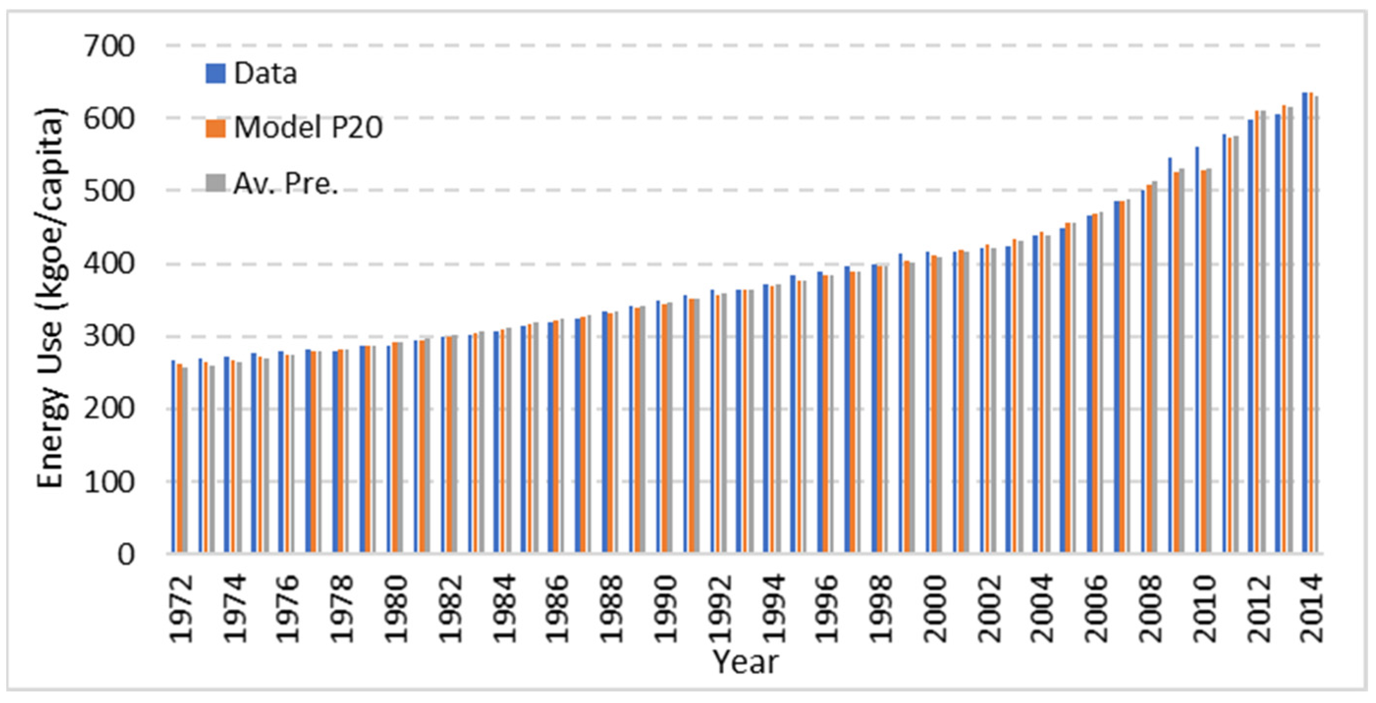
3.3. Verification of the Predictions Using Public Data

The comparison of predictions made from the algorithm was validated using the public data available for India [32] and referred to as energy use per person between 2015 and 2022. It is seen that the predicted energy use has a close association with the actual energy use, as depicted in Figure 13.

For the year 2022, the predicted energy use was found to be 780.02 kgoe/capita. Therefore, it was validated that the future predictions made based on the year-ahead prediction algorithm are significant, with a relative error of 2.63%.

4. Conclusions

The primary energy use has been modelled in terms of four socio-economic indicators, including GDP, population, and the values of exports and imports for India. The ensemble of Grammatical Evolution and Differential Evolution (GE-DE) was applied to the energy-use problems (estimation and prediction) on the historical data obtained from public websites from 1971 to 2014. Models were developed and compared with the help of statistical analysis comprising root mean square error, average error, coefficient of determination, absolute error, and relative error. Further, to establish the best of the models and create a ranking system, the Global Performance Index was applied. The models were deployed to estimate (for the estimation problem) and predict (for the year-ahead prediction problem) energy use. For any particular year, the energy use was defined by the median value, the first and third quartiles, and the minimum and maximum values. Based on the analysis, the following main conclusions were drawn:

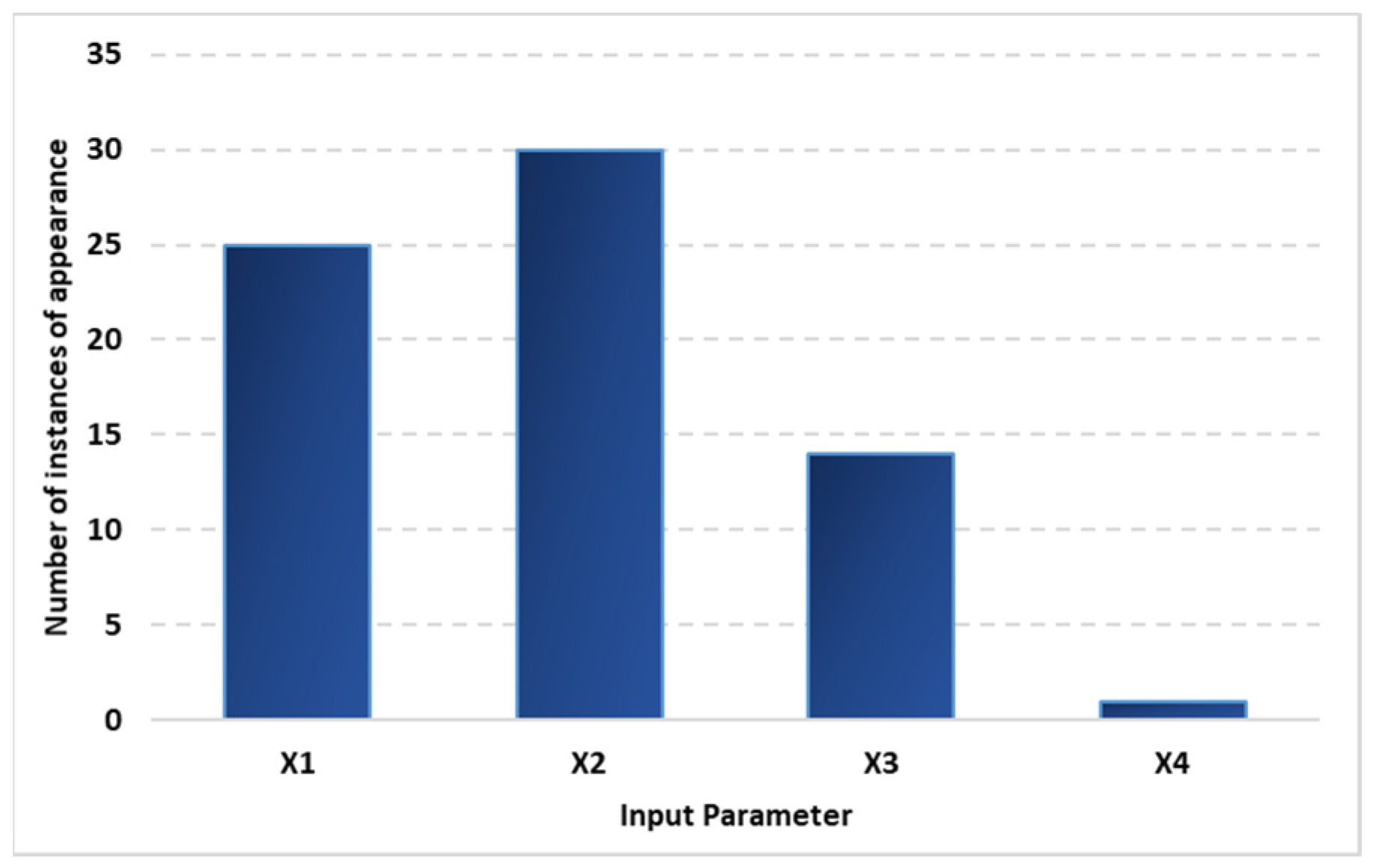
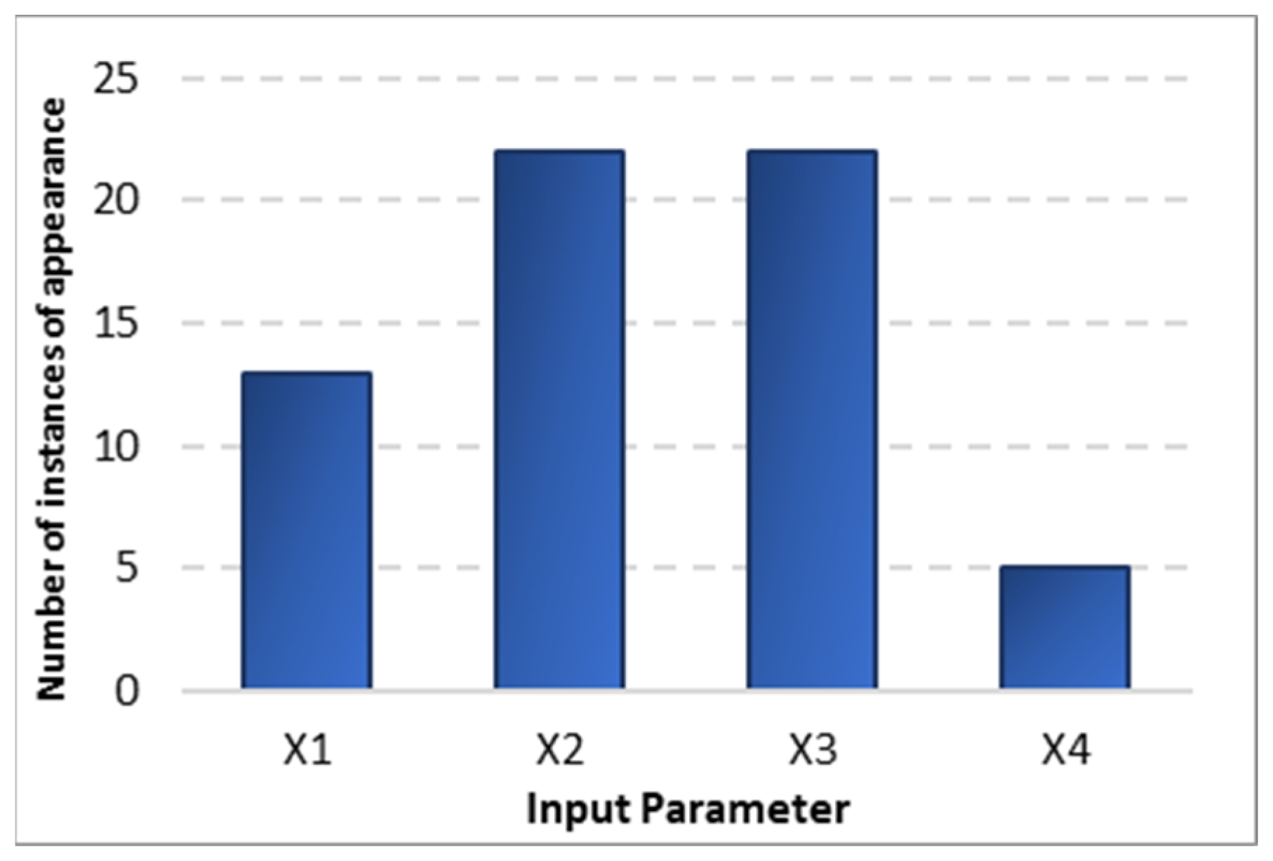
• The estimation of energy use based on the ensemble of GE-DE was found to have good accuracy, and the RMSE (based on average estimations) was quantified as 6.3749 kgoe/capita (1.25%). Based on the statistical analysis and the ranking established by GPI, Model E10 was the best model for the estimation with an RMSE and GPI of 5.8183 kgoe/capita and 1.7249, (meaning 1.03%). Population and GDP were found to have the highest number of instances of appearance in the estimation models and were, therefore, regarded as the influential parameters.
• The energy prediction problem, with a year-ahead prediction, was found to have a good agreement with the data, and the RMSE was obtained as 7.8857 kgoe/capita (1.56% error); model P20, with an RMSE of 7.9201 (or 1.42%) and a GPI of 1.8836, was found to be the most accurate. Population and the value of exports were found to be the most influential parameters for the case of prediction equations (based on the number of times they appeared).
• The predictions were further made for 2015–2022, and the results showed a slowdown in energy-use behaviour for 2020 and 2021. Further, a steady increase was found in energy use, with a median value of 770.29 kgoe/capita and an average value of 780.02 kgoe/capita.

Thus, it is established that the ensemble of GE-DE provides accurate estimation and prediction results and, therefore, can be applied to energy-use modelling as an optimization problem. Further work will be carried out to model the energy-use behaviour and project this energy use in the medium- to the long-term future under different growth scenarios.

It must, however, be considered that the models presented in the study have been developed and implemented as a case study for India. It is, therefore, recommended to verify the performance of the ensemble algorithms together with the country-specific data whenever predictions are made for any specific case. It should also be noted that the results of this study are based on annual data values; therefore, the derivatives of this study need to be extended to shorter time frames (monthly, weekly, or daily) with the appropriate data as available. Further, for future studies, it is recommended to consider a large number of datasets, in terms of the number of input parameters as well as the diversity of the regions, to generalize the results and to extend the study for wider cases.

References

1. Jiang, P.; Li, R.; Lu, H.; Zhang, X. Modeling of Electricity Demand Forecast for Power System. Neural Comput. Appl. 2020, 32, 6857–6875. [Google Scholar] [CrossRef]
2. Debnath, A.; Singh, S.V.; Singh, Y.P. Comparative Assessment of Energy Requirements for Different Types of Residential Buildings in India. Energy Build. 1995, 23, 141–146. [Google Scholar] [CrossRef]
3. Das, A.; Paul, S.K. Changes in Energy Requirements of the Residential Sector in India between 1993–94 and 2006–07. Energy Policy 2013, 53, 27–40. [Google Scholar] [CrossRef]
4. Dhawan, V.; Prasad, N. India: Transforming to a Net-Zero Emissions Energy System; The Energy and Resources Institute (TERI): Mithapur, India, 2020. [Google Scholar]
5. Parikh, K.S.; Karandikar, V.; Rana, A.; Dani, P. Projecting India’s Energy Requirements for Policy Formulation. Energy 2009, 34, 928–941. [Google Scholar] [CrossRef]
6. Chaturvedi, S.; Rajasekar, E.; Natarajan, S.; McCullen, N. A Comparative Assessment of SARIMA, LSTM RNN and Fb Prophet Models to Forecast Total and Peak Monthly Energy Demand for India. Energy Policy 2022, 168, 113097. [Google Scholar] [CrossRef]
7. Islam, M.A.; Che, H.S.; Hasanuzzaman, M.; Rahim, N.A. Chapter 5—Energy Demand Forecasting. In Energy for Sustainable Development; Hasanuzzaman, M.D., Rahim, N.A., Eds.; Academic Press: Cambridge, UK, 2020; pp. 105–123. ISBN 978-0-12-814645-3. [Google Scholar]
8. Löschel, A.; Managi, S. Recent Advances in Energy Demand Analysis—Insights for Industry and Households. Resour. Energy Econ. 2019, 56, 1–5. [Google Scholar] [CrossRef]
9. Huang, C.; Zhang, Z.; Li, N.; Liu, Y.; Chen, X.; Liu, F. Estimating Economic Impacts from Future Energy Demand Changes Due to Climate Change and Economic Development in China. J. Clean. Prod. 2021, 311, 127576. [Google Scholar] [CrossRef]
10. Wang, H.; Chen, Z.; Wang, W.; Wu, Z.; Wu, K.; Li, W. Improving Energy Demand Estimation Using an Adaptive Firefly Algorithm BT—Computational Intelligence and Intelligent Systems; Li, K., Li, W., Chen, Z., Liu, Y., Eds.; Springer: Singapore, 2018; pp. 171–181. [Google Scholar]
11. Jamil, B.; Serrano-Luján, L.; Colmenar, J.M. On the Prediction of One-Year Ahead Energy Demand in Turkey Using Metaheuristic Algorithms. Adv. Sci. Technol. Eng. Syst. J. 2022, 7, 79–91. [Google Scholar] [CrossRef]
12. Sajadi, S.M.; Asadzadeh, S.M.; Majazi Dalfard, V.; Nazari Asli, M.; Nazari-Shirkouhi, S. A New Adaptive Fuzzy Inference System for Electricity Consumption Forecasting with Hike in Prices. Neural Comput. Appl. 2013, 23, 2405–2416. [Google Scholar] [CrossRef]
13. Majazi Dalfard, V.; Nazari Asli, M.; Nazari-Shirkouhi, S.; Sajadi, S.M.; Asadzadeh, S.M. Incorporating the Effects of Hike in Energy Prices into Energy Consumption Forecasting: A Fuzzy Expert System. Neural Comput. Appl. 2013, 23, 153–169. [Google Scholar] [CrossRef]
14. Daş, G.S. Forecasting the Energy Demand of Turkey with a NN Based on an Improved Particle Swarm Optimization. Neural Comput. Appl. 2017, 28, 539–549. [Google Scholar] [CrossRef]
15. Salcedo-Sanz, S.; Muñoz-Bulnes, J.; Portilla-Figueras, J.A.; Del Ser, J. One-Year-Ahead Energy Demand Estimation from Macroeconomic Variables Using Computational Intelligence Algorithms. Energy Convers. Manag. 2015, 99, 62–71. [Google Scholar] [CrossRef]
16. Sánchez-Oro, J.; Duarte, A.; Salcedo-Sanz, S. Robust Total Energy Demand Estimation with a Hybrid Variable Neighborhood Search—Extreme Learning Machine Algorithm. Energy Convers. Manag. 2016, 123, 445–452. [Google Scholar] [CrossRef]
17. Duran Toksarı, M. Ant Colony Optimization Approach to Estimate Energy Demand of Turkey. Energy Policy 2007, 35, 3984–3990. [Google Scholar] [CrossRef]
18. Ünler, A. Improvement of Energy Demand Forecasts Using Swarm Intelligence: The Case of Turkey with Projections to 2025. Energy Policy 2008, 36, 1937–1944. [Google Scholar] [CrossRef]
19. Yu, S.; Wei, Y.-M.; Wang, K. A PSO–GA Optimal Model to Estimate Primary Energy Demand of China. Energy Policy 2012, 42, 329–340. [Google Scholar] [CrossRef]
20. Wang, Q.; Li, S.; Li, R. Forecasting Energy Demand in China and India: Using Single-Linear, Hybrid-Linear, and Non-Linear Time Series Forecast Techniques. Energy 2018, 161, 821–831. [Google Scholar] [CrossRef]
21. Özdemir, D.; Dörterler, S.; Aydın, D. A New Modified Artificial Bee Colony Algorithm for Energy Demand Forecasting Problem. Neural Comput. Appl. 2022, 7, 17455–17471. [Google Scholar] [CrossRef]
22. Incremona, A.; De Nicolao, G. Short-Term Forecasting of the Italian Load Demand during the Easter Week. Neural Comput. Appl. 2022, 34, 6257–6271. [Google Scholar] [CrossRef]
23. Torres, J.F.; Martínez-Álvarez, F.; Troncoso, A. A Deep LSTM Network for the Spanish Electricity Consumption Forecasting. Neural Comput. Appl. 2022, 34, 10533–10545. [Google Scholar] [CrossRef]
24. Li, R.; Chen, X.; Balezentis, T.; Streimikiene, D.; Niu, Z. Multi-Step Least Squares Support Vector Machine Modeling Approach for Forecasting Short-Term Electricity Demand with Application. Neural Comput. Appl. 2021, 33, 301–320. [Google Scholar] [CrossRef]
25. Stergiou, K.; Karakasidis, T.E. Application of Deep Learning and Chaos Theory for Load Forecasting in Greece. Neural Comput. Appl. 2021, 33, 16713–16731. [Google Scholar] [CrossRef]
26. Michell, K.; Kristjanpoller, W.; Minutolo, M.C. Electrical Consumption Forecasting: A Framework for High Frequency Data. Neural Comput. Appl. 2022, 34, 5577–5586. [Google Scholar] [CrossRef]
27. Mohammed, N.A.; Al-Bazi, A. An Adaptive Backpropagation Algorithm for Long-Term Electricity Load Forecasting. Neural Comput. Appl. 2022, 34, 477–491. [Google Scholar] [CrossRef] [PubMed]
28. IBRD IDA. The World Bank Data. Available online: https://databank.worldbank.org/home.aspx (accessed on 11 August 2022).
29. O’Neill, M.; Ryan, C. Grammatical Evolution. IEEE Trans. Evol. Comput. 2001, 5, 349–358. [Google Scholar] [CrossRef]
30. Despotovic, M.; Nedic, V.; Despotovic, D.; Cvetanovic, S. Review and Statistical Analysis of Different Global Solar Radiation Sunshine Models. Renew. Sustain. Energy Rev. 2015, 52, 1869–1880. [Google Scholar] [CrossRef]
31. MacroTrends Global Metrics. Available online: https://www.macrotrends.net/ (accessed on 10 October 2022).
32. Ritchie, H.; Roser, M.; Rosado, P. Energy. Available online: https://ourworldindata.org/energy (accessed on 15 October 2022).
Figure 1. Outline of the methodology followed under the present work.
Energies 17 01697 g001
Figure 2. Schema of ensemble algorithmic methods (GE-DE).
Energies 17 01697 g002
Figure 3. Recursive grammar-driven GE-DE ensemble.
Energies 17 01697 g003
Figure 4. Number of instances of appearance of different input parameters in the estimation models.
Energies 17 01697 g004
Figure 5. Comparison of estimated energy use vs. the target values (normalized) on (a) training dataset and (b) testing dataset.
Energies 17 01697 g005
Figure 6. Evolution of estimated energy use for 1971–2014, showing the variability of the 20 models obtained: median energy-use value, first and third quartiles, and minimum and maximum values.
Energies 17 01697 g006
Figure 7. Comparison of actual energy use with the estimated (Model E10) and the energy use estimated as an average from the twenty models.
Energies 17 01697 g007
Figure 8. Number of instances of appearance of input variables in the prediction models.
Energies 17 01697 g008
Figure 9. Comparison of year-ahead predicted energy use vs. the target values (normalized) on the (a) training dataset and (b) testing dataset.
Energies 17 01697 g009
Figure 10. Evolution of predicted year-ahead energy use for 1972–2014 and further for the predicted year 2015.
Energies 17 01697 g010
Figure 11. Comparison of actual energy use with the predicted (Model P20) and the average of twenty prediction models.
Energies 17 01697 g011
Figure 12. Predicted energy use for the period of 2015–2022.
Energies 17 01697 g012
Figure 13. Comparison of predicted values of energy use from the algorithms with the public data available from 2015 through 2022.
Energies 17 01697 g013