Article

A Dependability Neural Network Approach for Short-Term Production Estimation of a Wind Power Plant

by
Fabio Famoso
1,
Ludovica Maria Oliveri
2,
Sebastian Brusca
1 and
Ferdinando Chiacchio
2,*
1
Department of Engineering, University of Messina, 98166 Messina, Italy
2
Department of Electrical, Electronic and Computer Engineering, University of Catania, 95125 Catania, Italy
*
Author to whom correspondence should be addressed.
Energies 2024, 17(7), 1627; https://doi.org/10.3390/en17071627
Submission received: 8 March 2024 / Revised: 20 March 2024 / Accepted: 26 March 2024 / Published: 28 March 2024
(This article belongs to the Special Issue Volume Ⅱ: Advances in Wind and Solar Farm Forecasting)

Abstract

:
This paper presents a novel approach to estimating short-term production of wind farms, which are made up of numerous turbine generators. It harnesses the power of big data through a blend of data-driven and model-based methods. Specifically, it combines an Artificial Neural Network (ANN) for immediate future predictions of wind turbine power output with a stochastic model for dependability, using Hybrid Reliability Block Diagrams. A thorough state-of-the-art review has been conducted in order to demonstrate the applicability of an ANN for non-linear stochastic problems of energy or power forecast estimation. The study leverages an innovative cluster analysis to group wind turbines and reduce the computational effort of the ANN, with a dependability model that improves the accuracy of the data-driven output estimation. Therefore, the main novelty is the employment of a hybrid model that combines an ANN with a dependability stochastic model that accounts for the realistic operational scenarios of wind turbines, including their susceptibility to random shutdowns This approach marks a significant advancement in the field, introducing a methodology which can aid the design and the power production forecast. The research has been applied to a case study of a 24 MW wind farm located in the south of Italy, characterized by 28 turbines. The findings demonstrate that the integrated model significantly enhances short-term wind-energy production estimation, achieving a 480% improvement in accuracy over the solo-clustering approach.

1. Introduction

Climate change is prompting more frequent extreme weather events globally, driving Europe to actively pursue the 2030 Agenda to combat pollution and environmental degradation. Achieving the Intergovernmental Panel for Climate Change (IPCC) goal of limiting global warming to 1.5 °C, and reaching carbon neutrality by mid-century is essential, as per the Paris Agreement [1], ratified by 195 countries, including the EU. The European Commission’s European Green Deal [2] in December 2019 aims for climate neutrality by 2050. This includes enhancing the fit for 55 proposals to increase renewable energy and efficiency targets [3], with plans under “Electrify Europe” [4] for deploying 480 GW of wind and 420 GW of solar capacities. The “REPowerEU” strategy [3] seeks to frontload wind and solar development by 20%, adding 80 GW by 2030 for renewable hydrogen production. The role of production estimation in renewable energy, crucial for strategic planning and ensuring a stable power supply despite the variability of renewable sources, highlights the necessity for meticulous network planning.
In the last decade, the global wind energy sector has experienced remarkable growth, expanding by an average of over 30% annually, as reported by the Global Wind Energy Council (GWEC) [5]. Maintaining this growth trajectory could result in wind energy meeting nearly one-third of the world’s electricity needs by 2050. As discussed in [6], the wind energy industry stands out as the fastest-growing infrastructure worldwide, with promising prospects also because its generation costs have significantly declined over the past 15 years. This trend applies both to offshore and onshore [7] installations, nearing parity with traditional energy sources. Consequently, this phenomenon has encouraged the scientific community to better assess estimation methods for wind energy production [8]. Wind power generators are characterized by inherent variability in wind speed and direction, and this makes it challenging to assess wind power generation using conventional methods. Time horizon plays a crucial role in model accuracy, with estimation errors typically increasing as the time range extends [9], affecting also the maintenance plan of such complex machines. Estimation methods are categorized based on the time range for different aims. Short-term methods (1 to 96 h) are employed for power system planning, dispatch, and electricity trading. Medium-term methods (96 h to 1 week) are utilized for scheduling maintenance of energy storage systems. Long-term methods (weeks to months) are employed to evaluate wind farm overall energy production and investment payback [10,11,12]. Thus, engineering models are variegated. Physical models utilize global meteorological databases or atmospheric models, requiring extensive computational systems for accurate results [13,14]. Statistical methods analyze vast amounts of data without representing meteorological processes, yielding good results for mean monthly or higher temporal-scale wind speed estimation [15]. Learning approaches, or AI data-driven models, serve as a compromise, explaining physical phenomena without relying on a physical model. However, these methods face challenges in near-real-time performance due to increased computational load of data time series and observations [9]. In light of these outlined challenges, this study centers on a pivotal question: can data-driven methods based on an ANN maintain high accuracy with a reduced set of data, for the short-term estimation of wind farm energy production? This inquiry is crucial for developing real-time, efficient energy estimation methods that reconcile computational demands with the operational intricacies of wind power generation.
This study introduces a novel method for the short-term estimation of the energy produced by a wind farm. This methodology adopts the combination of a multilayer perceptron (MLP) artificial neural network (ANN) [10,16] and the dependability model of the wind turbines. This approach marks a significant advancement in the field, introducing a hybrid model that merges a data-driven AI technique with a model-based strategy, thereby contributing a novel solution to the existing body of research.
The paper is structured as follows: Section 2 offers a comprehensive overview of the current state of the art, setting the context for the paper’s contributions. Section 3 introduces the main components of the hybrid methodology, encompassing both the data-driven approach and the model-based theory of dependability and reliability. Section 4 delves into the case study, detailing the experimental campaign and presenting the achieved results. Finally, Section 5 concludes the paper with remarks and a discussion on limitations, and envisions avenues for future research.

2. State of the Art

Effective production estimation in renewable energy plays a pivotal role across various domains, significantly influencing planning, management, and integration within the broader energy landscape. Accurate predictions of energy output from renewable sources, such as solar and wind, are crucial for the strategic planning and operation of power grids. The variability inherent in renewable sources requires careful network planning to handle fluctuations and ensure a consistent power supply, avoiding overload and instability [17].
Moreover, production estimations are instrumental in seamlessly integrating renewable energies into the overall energy supply. As these sources often depend on weather conditions, precise estimation facilitates efficient balancing of production and consumption [18]. This integration is pivotal for optimizing the overall efficiency and reliability of the energy grid.
Operational efficiency is a key consideration for energy sector entities, including operators of renewable energy facilities. Accurate production estimations enable these organizations to plan operational activities effectively, including scheduled maintenance [19], production optimization, and human resource management [20]. The reduction in electricity costs is a significant benefit stemming from accurate production estimation. By minimizing the need for excess backup energy and optimizing resource utilization, production estimations contribute to the overall economic efficiency of the energy system [21]. In this way, companies can enhance overall efficiency and resource allocation [22] with strategic investments in energy infrastructure which, in turn, aids in the broader goal of transitioning towards sustainable and renewable energy sources.
In [23], Lee and Fields emphasize the historical tendency of the wind industry to overpredict the annual energy production of wind farms, leading to significant financial implications. To address this bias, over the past few decades, there has been widespread development and successful application of various methodologies in predicting wind energy. In general, these approaches can be classified into model-based and data-driven methods [24,25,26]. Model-based methods utilize physics models that incorporate wind forecasting data for predicting wind energy outcomes [27,28,29,30]. In a previous work, authors have proposed a hybrid model to combine the Jensen wake mathematical theory with a stochastic dependability model to improve the accuracy of energy production in a long-term period [31]. On the other hand, data-driven approaches eschew explicit physical models and exclusively rely on wind data to construct (black-box) models capturing the relationship between wind-forecasting data and the corresponding wind energy production [32,33,34,35,36]. In recent decades, numerous data-driven techniques have gained prominence in the field of wind energy prediction. Noteworthy examples include Artificial Neural Networks (ANNs) [37,38,39,40]; Support Vector Machines (SVMs) [27,38,41,42]; k-nearest neighbors (kNN) regression [39,43,44]; Support Vector Regression (SVR) [29,45]; and Gaussian Process Regression (GPR) [38,46]. Such methodologies have been successfully applied also to the field of predictive maintenance, where [47] shows that a dynamic dependability model can be used to produce additional dataset for training AI predictors and estimate the remaining useful life of general steel components.
Sanchez, in [48], introduces a statistical forecasting system for wind energy prediction based on the adaptive combination of alternative dynamic models. This flexibility is achieved through the utilization of alternative models based on different assumptions about the involved variables, the adaptive estimation of their parameters using diverse recursive techniques, and the implementation of an online adaptive time-varying forecast combination scheme, where both the number of predictors and their weights vary over time to derive the final prediction.
To quantify the possible sources of uncertainty that affect the predictions of wind energy production provided by an ensemble of ANN models, [49] proposes the Bootstrap (BS) technique for uncertainty quantification, relying on estimating Prediction Intervals (PIs) for a predefined confidence level.
The optimal model probably consists in a mixed approach, which is very often adopted by utilities to combine high accuracy for very short horizons together with longer forecasts of up to 48–72 h. In [50], Cassola et al. focus on a mixed approach based on the use of a Numerical Weather Prediction (NWP) model coupled to a statistical model based on the Kalman filtering technique. They underline the fact that by tuning the time-step and the forecast horizon of the filter, this methodology is capable of providing a significant improvement in estimation with respect to the wind-speed-model direct output, especially when used for very short-term estimation. Table 1 presents a categorization of papers included in the literature review based on the adopted methodological approach and model used. Approaches are differentiated into Data-Driven, Model-Based, and Hybrid categories, to provide an organized overview.
Meteorological station data serves as the foundation for several influential studies investigating the effects of renewable resource variability, such as those conducted by Cox [52] and Sinden [53]. Kubik et al. [54] discovered that employing a single wind shear coefficient throughout the entire year, a common practice in simulated wind generation models, yields a reliable estimate for annual energy production. However, they noted that errors related to specific hours could be significant. In this research work, meteorological data were employed as input variables to train the neural network, avoiding the introduction of any coefficients, and thus reducing the error in calculating the power generated by the wind farm.
In their study, Wang et al. [55] emphasized that considering the impact of multivariate historical meteorological factors, including wind speed, wind direction, and ambient temperature, on wind power output helps enhance forecasting performance. Consistent with this study, this paper considered both wind speed and direction.
As demonstrated by a rich literature [32,34,37,49], ANNs have already been applied for non-linear stochastic problems of energy, power or weather forecast estimation. In this study, the primary innovation of employing an ANN lies in its ability to significantly reduce computational efforts by simplifying the elements involved in processing, while still delivering accurate energy production estimates. These results are further improved by integrating a dependability stochastic model that accounts for the realistic operational scenarios of wind turbines, including their susceptibility to random shutdowns. The review in [56] present several papers regarding the use of machine learning for optimizing the maintenance planning of wind energy systems.
The literature review was conducted using Mendeley and Scopus, inputting the queries “wind AND turbin* AND model-based AND dependability AND analyses AND machine AND learning AND methods” and “wind AND turbin* AND power AND estimation AND dependability OR stochastic AND artificial AND neural AND network”. No articles discussing the approach presented in this work were found.
The literature reveals a gap in integrating machine learning methods with model-based dependability analyses of wind turbines. This paper aims to bridge this gap by proposing a hybrid data-driven methodology that incorporates dependability aspects for the short-term energy estimation of wind power plant production. Moreover, the methodology proposed simplifies the process of assessing wind farm productivity potential during the site selection phase. Specifically, engineers have the option to minimize the quantity of anemometers deployed in the design stage by strategically situating them at locations corresponding to the centroid turbines of identified clusters. This approach not only simplifies the initial engineering tasks, but also offers potential cost reductions in terms of equipment and labor needed for site assessment.

3. Methodology

This section outlines the methodology employed for short-term forecasting of power and energy output in wind power plants. As illustrated in Figure 1, the proposed model integrates two distinct algorithms: a data-driven module, structured into three stages, and a dependability module that employs stochastic modeling to assess the reliability and availability of wind turbine generators (WTGs).
The approach is designed for efficiency in data usage, relying on available wind speed and direction forecasts and focusing on data from select ‘centroid turbines’ rather than the entire array. This targeted data collection reduces the volume of necessary input data, enhancing computational efficiency. The integration of a dependability model further improves the accuracy of predictions, offering a comprehensive view of potential energy output while maintaining precision in estimations.
Therefore, the methodology presents the following advantages:
-
Reduced Computational Effort: by focusing on key turbines, the approach lessens the computational load, enabling faster, more efficient processing.
-
High Precision: the combination of the dependability model with the data-driven module guarantees high accuracy in forecasting energy production, even with fewer data inputs.
However, the methodology’s primary disadvantage lies in its strong dependence on wind forecasts. In other words, the success and accuracy of predictions rely heavily on the availability and precision of wind speed and direction forecasts, which may require significant infrastructure and investment in forecasting technologies. This issue is, somehow, reduced thanks to the utilization of centroid turbines, as discussed next.

3.1. Data-Driven Model

The Data-Driven Model used in this paper takes inspiration from the classic methodologies of machine learning and Artificial Intelligence. As it can be seen in Figure 1, a pre-processing analysis has to be performed before feeding the Artificial Neural Network, which represents the final layer of the Data-Driven Model. This latter is in charge of performing the actual short-term estimation of the wind farm. As far as it concerns the Data-Driven algorithm, the main novelty proposed in this paper is the adoption of an ad hoc Cluster Analysis, in the second step of this module. The Cluster Analysis is tailored to the wind farm because it makes use of Geographic Information System (GIS) information of the wind turbines, including the terrain orography of the power plant site; this allows for the simplification of the computation of the Neural Network.

3.1.1. Pre-Processing Analysis

The pre-processing analysis is a crucial step for the data-driven algorithm, as it involves gathering and cleaning the data necessary for creating clusters of wind turbines and training the neural network. This step entails collecting data from all turbines in the power plant farm, followed by data pre-processing and standardization of statistical values. Initially, the process begins with georeferencing the wind turbines using a GIS-based system to enable geographical clustering.
For each wind turbine, variables such as power output, wind speed, and wind direction are collected through time-series samples from available data sources (e.g., Supervisory Control and Data Acquisition SCADA, and the Distributed Control System DCS). During this phase, data pre-processing analysis, such as applying moving averages, may be utilized to correct missing or incorrect values.
Subsequently, statistical metrics including mean and standard deviation (σ) of power output, wind speed, and wind direction are computed for each turbine over a time interval. The time interval must be chosen, for the sake of convenience in data transformation, to be a multiple of the interval of the data sample time-step of the time-series (typically, SCADA systems in wind power plants offer ten-minute intervals).
Given the significant scale differences among these variables, a standardization step is critical for the next phase of the cluster analysis. This standardization facilitates the comparison of scores, regardless of their differing measurement scales. The primary criterion for this process makes use of the following transformation:
Z X = X m σ
where Z(X) is the standardized value, X is the variable that has to be standardized, m is the mean and σ is the standard deviation.

3.1.2. Cluster Analysis

The aim of cluster analysis is to group wind turbines into homogeneous clusters. Each wind turbine can be characterized by its GIS coordinates and the statistical data obtained during the pre-processing analysis, which involves six variables: the mean and standard deviation of the power output, wind speed, and wind direction. Thus, the wind turbines can be represented in a multi-dimensional space (defined by the 6 variables, plus the latitude, longitude and altitude retrieved by the GIS georeferencing), where each point in the 9-dimensional space represents a turbine. The center of the n-dimensional space, the centroid, is calculated using Euclidean distance. The turbine closest to the centroid is selected, representing the cluster most accurately.
The two-step cluster analysis is extensively applied in a variety of environmental research contexts [57,58]. This algorithm falls under the hierarchical clustering category and consists of two stages:
  • A pre-clustering that examines the data sample of each individual element (e.g., the wind turbine) to determine whether it can be integrated into an existing cluster or if it should serve as the centroid for a new cluster. This decision is based on a specific distance criterion. For the proposed model, the Euclidean distance was selected as the distance criterion, defined as follows:
    E d T 1 , T 2 =   i = 1 n T i 1 T i 2 2
    where T i k is a tuple T i k   = ( T 1 k , T 2 k , …, T n k ) characterized by n variables. In these cases, T i k represents the generic “k” wind turbine modeled by the 9 standardized variables (i   1 ; 9 ) .
  • The clustering validity analysis is the step of the algorithm that determines the dimension and the number of elements of each cluster. This algorithm can iteratively perform a grouping with different sizes of elements. In order to select the most appropriate number of clusters, the silhouette (S) coefficient is used:
    S i = b i a i max a i , b i
In this methodology, ai represents the mean distance between the ith data point and all other points within the same cluster, whereas bi denotes the smallest average distance from the ith to all points in any other cluster that does not include the ith point. If the value of S is greater than 0.5 the cluster can be considered as coherent (wind turbines are homogeneous with each other).
Therefore, in order to lower the computational effort, the smallest number of clusters that satisfy the coherence criteria is selected and a representative turbine for each cluster is selected. This selection is based on identifying the turbine with the smallest Euclidean distance from the centroid of its respective cluster.

3.1.3. Artificial Neural Network Estimation Step

In this study, a Multilayer Perceptron (MLP) neural network is employed to perform the short-term estimation of the wind power plant productivity. Multilayer Perceptron is particularly suited for addressing complex nonlinear problems like wind power estimation [32,33,37]. The network adopts a feedforward architecture and consists of three layers: an input layer, a hidden layer, and an output layer. With the exception of the input nodes, each node functions as a neuron that employs a nonlinear activation function. Specifically, the sigmoid function was chosen for its historical prevalence in neural network applications.
The neural network architecture employed in this study, an MLP, features an input layer designed with a number of neurons that corresponds to the total number of wind turbines in the farm. It uses a supervised learning method known as backpropagation for training purposes. In the training phase, this network is supplied with datasets containing wind speed and direction for each turbine, effectively modeling each turbine’s contribution to the farm’s overall power output. This process relies on supervised learning, necessitating prior knowledge of the wind farm’s actual power output for accurate model adjustment. During the subsequent testing phase, the network is challenged to predict the farm’s power output using only the input data on wind conditions. In the development of the MLP model, careful consideration was given to the dataset’s preparation and the network’s training and testing conditions to ensure optimal predictive performance. The dataset was divided into 70% for training and 30% for testing, a split that is widely recognized in machine learning practices for offering a balanced approach to model training and generalizability assessment. This ratio allows for comprehensive learning from a substantial portion of the data while retaining a significant subset for unbiased evaluation of the model’s predictive capability on unseen data. Further, a temporal data splitting strategy was employed, allocating 10 days for model training followed by 4 days for testing. Such a temporal split results in 1440 training samples and 576 testing samples, considering a sampling rate of 1 data point every 10 min, thereby ensuring that the model is well-adjusted to both the frequency and variability of wind farm data.
Additionally, to enhance the model’s efficiency and accuracy, we leveraged the Matlab® (Version R2022B) Deep Learning Toolbox, which offers a comprehensive suite of functions and tools designed to optimize neural networks. These methodological choices—spanning data splitting, temporal allocation for training and testing, and Matlab optimization—are designed to strike a delicate balance between learning complexity and prediction capability.
As demonstrated in the experimental section of the case study, the objective of the pre-processing and cluster analysis is to reduce the number of wind turbines (correspondingly, the input layer neurons) in the neural network, thereby alleviating the computational load of the methodology.

3.2. Model-Based Dependability

One of the main attributes of dependability is reliability, which measures the probability of a system working with no failures for the entire time of observation, known as mission time. The mathematical formulation of system reliability is shown in Equation (4):
R = e 0 t h τ d τ
where h(τ) is known as the instantaneous failure rate of the system. This function serves to quantify the probability of a failure occurring within a given time interval, given that no failure has occurred prior to time t [59].
Figure 2 shows the bathtub curve, a more general model for the instantaneous failure rate property h(τ) of a generic component, where it is possible to identify three main regions:
-
Early failures: where h(τ) decreases with time. This phase contributes to removing all the components which do not pass the trial stage, so that components are not placed on the market.
-
Random failures: where it is assumed that only random failures can occur. This is the phase that characterizes the useful life of a component, assuming that this failure rate is constant (this represents a general limitation of reliability models).
-
Deterioration: where h(τ) is increasing due to deterioration. This region corresponds to the phase where the component is old and should be replaced with a new component.
The three regions of the bathtub curve can be modelled by means of the Weibull density function, which depends on two parameters, the scale factor α and the shape parameter β:
h t = β α β t β 1
If β = 1, the h(t) is constant with λ = 1/α; otherwise, with β > 1 h(t) it is increasing and with β < 1 h(t) it is decreasing.
Figure 2. The bathtub model of the instantaneous failure rate (β is the shape parameter of a Weibull distribution).
Energies 17 01627 g002
The ‘random failures region’ refers to a phase in the system’s life known as its useful lifetime, during which the system primarily experiences random failures. These random failures are assumed to occur unpredictably and can be accurately described using an exponential distribution. This assumption allows the instantaneous failure rate to be considered constant over time, denoted as h(t) = λ [60]. This leads to a simplified equation for reliability which calculates the probability that the system will function without failure up to time t:
R t = e λ t
This simplified model is particularly useful when dealing with complex machinery composed of many parts. Engineers and risk management professionals often rely on it for its straightforwardness and practicality. The constant failure rate (λ) is determined based on manufacturer recommendations and the historical data of similar or equivalent components [58,61,62,63]. In the context of wind turbines, for instance, several studies focus on compiling the failure rates of various components to establish an average failure rate [64]. This approach allows for a more manageable analysis of the causes behind wind turbine failures, offering a way to aggregate component data and better understand overall system reliability.
Equation (7) shows the equation for the reliability when the Weibull probability function is used:
R t = e 1 α t β
Depending on the stochastic behavior, the failure of a component is sometimes modelled by means of the normal distribution, characterized by two parameters: μ is the mean time to failure and σ is the standard deviation. In this case, the integration of Equation (8) must be performed numerically:
R t = t 1 σ 2 π   e 1 2 τ μ σ 2 d τ
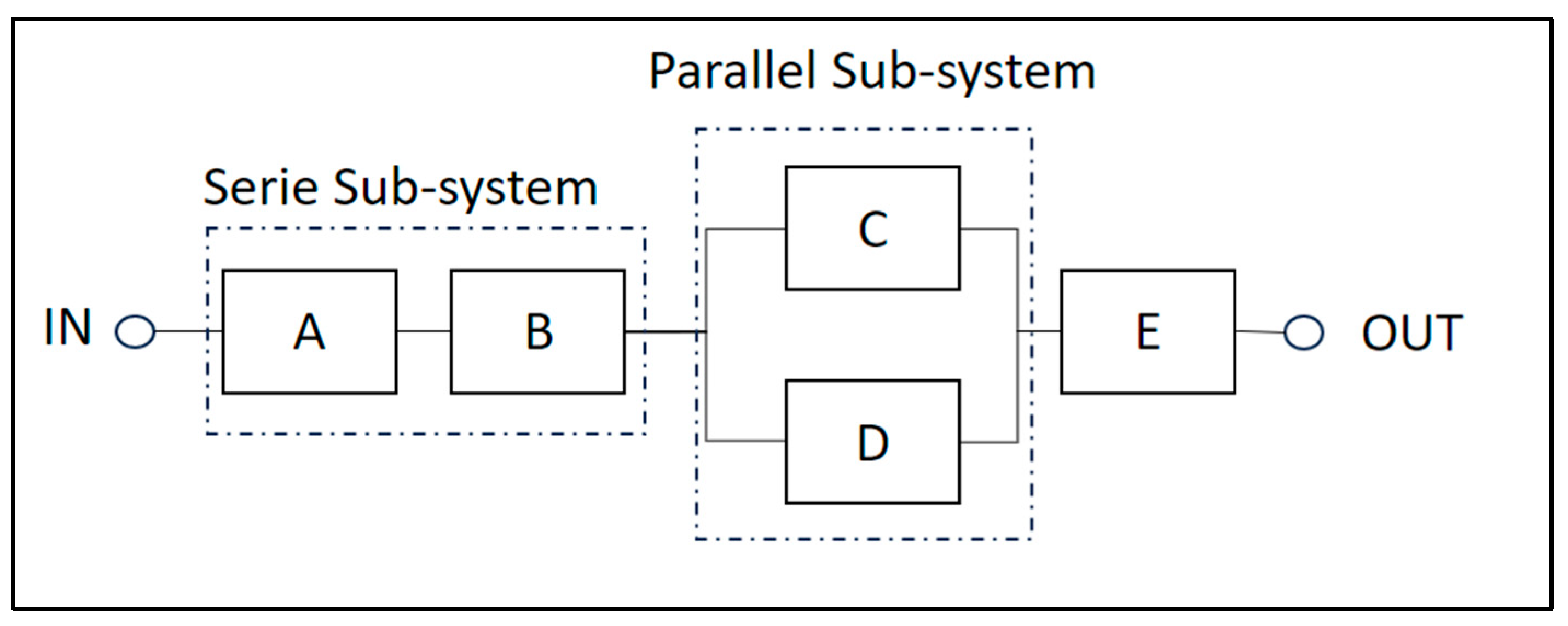
Since the mathematical dependability formulation of a complex system is not easy to formulate, high-level methodologies, such as Reliability Block Diagrams (RBD) are often used in the industrial field. This methodology helps in modeling and assessing the reliability of systems comprised of interconnected components, aiding in the identification of critical paths, potential failure points, and overall system vulnerabilities. In an RBD, system components are represented by blocks, each denoting a distinct element contributing to the overall functionality. Blocks can encompass a variety of components, ranging from simple elements to entire subsystems. Connections of blocks, reflecting different modes of component interaction, may be in series or parallel, forming the RBD paths. For the system/process to work there may exist a path from the node IN to the node OUT.
In the example of Figure 3, the RBD is made up of five components; A and B constitute a series subsystem, and C and D constitute a parallel subsystem. These two subsystems are in series with the component E.
The reliability of each block is generally modelled by means of a mathematical formulation (see Equations (5)–(8)) that depends on the component (or subsystem) failure characteristics. Finally, the reliability of the system/process can be computed by calculating the probability of all the paths of the RBD.
One of the main limitations of this methodology is the incapability of modeling environmental conditions and variable operational parameters. Clearly, in the field of renewable power plants [35], this represents an important drawback considering the randomness of primary resources (wind, sun, etc.) and their dependency with regard to the operations of these systems. To tackle this issue, this paper proposes the adoption of hybrid blocks that can vary their failure characteristics according to the operational conditions of the system.
In this paper, the modeling of the Hybrid Reliability Block Diagram (HBRD) has been realized by exploiting the Stochastic Hybrid Fault Tree Object Oriented (SHyFTOO) library [64], a Monte Carlo simulation engine that allowed for the modification of the failure/repair rate of wind turbines. In fact, as discussed in [65,66], the threshold value of 20 m/s defines a limit between two different failure probability density functions, for each component of the wind turbine. This concept will be further developed in the case study model of Section 4.

4. Case Study and Results

This section describes the case study and the results obtained with the methodology introduced in Section 3. In Section 4.1, the wind farm is described; in Section 4.2 and Section 4.3, the results of the power estimation with the sole data-driven algorithm are presented. Finally, Section 4.4 shows the results by coupling the data-driven model with the dependability model of a wind turbine, utilizing the Hybrid Reliability Block Diagram model. As discussed in Section 4.5, the hybrid model enhances the accuracy of the algorithm estimations.

4.1. Wind Farm

The wind farm object of this case study is located in the southern Italy. It presents a total out power (Pout) of 24 MW with 28 identical wind turbines. The wind farm is situated in a mountainous area, with varying altitudes for each turbine. Additional key details are provided in Table 2.
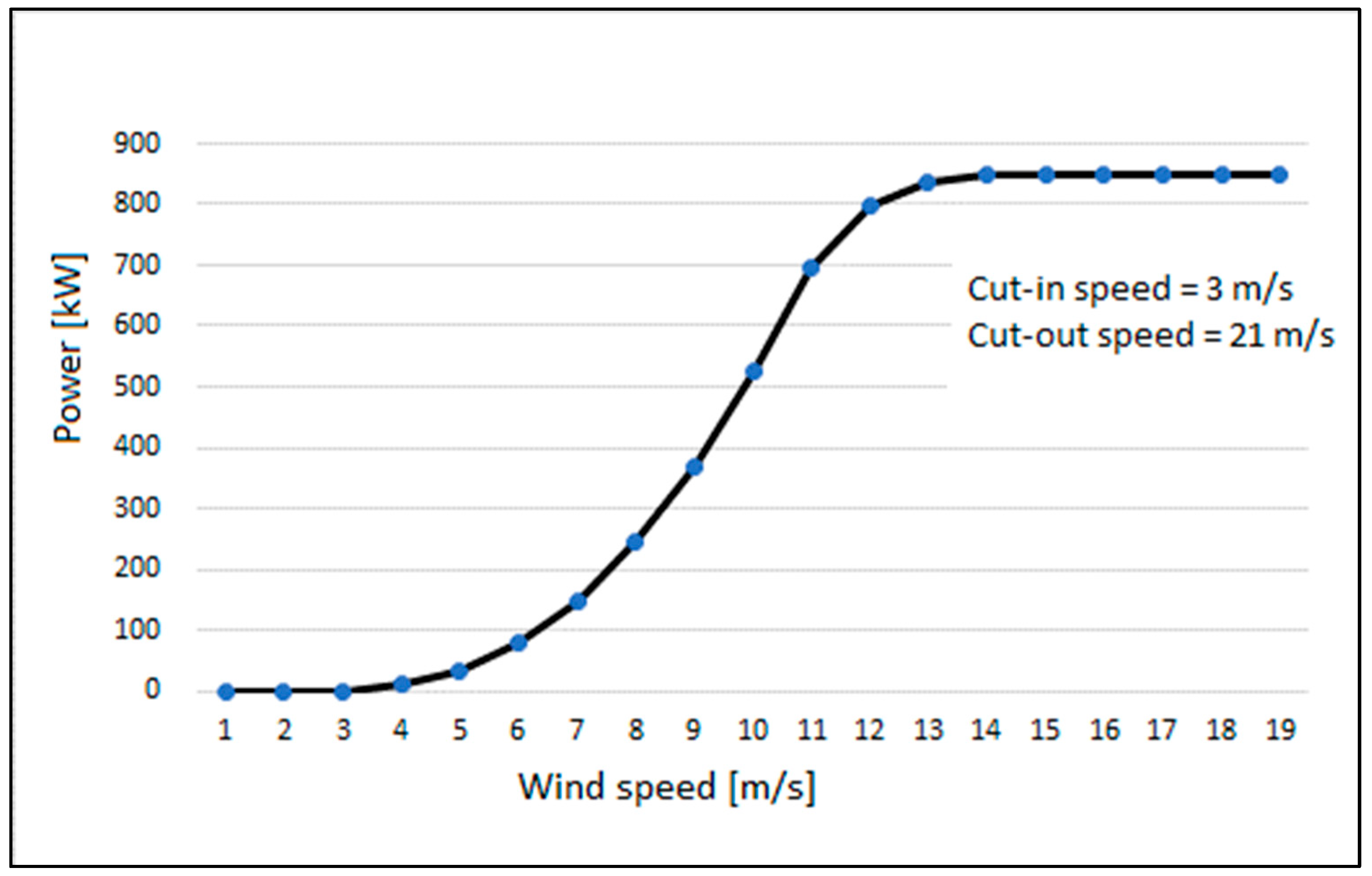
The turbine model presents a power curve with a very low cut-in speed, as reported in Figure 4. The choice of this turbine model is probably due to the low wind speed distribution of that geographical zone. Figure 5 illustrates the layout of the wind farm.
The dataset of the wind power plant is provided by a second-level SCADA with a sampling time-step of 10 min. The data presented a percentage of missing samples of around 1% that were cleaned with the pre-processing step of the algorithm.
Table 3 shows, as an example, the main values of the mean and the standard deviation for a subset of turbines (one per cluster). As discussed in Section 3.1.1., the mean and standard deviation of these variables (Pout, Wind speed and Wind Direction) are retrieved by the pre-processing analysis. This set of data is then used in the cluster analysis to group the wind turbines.
As far as the wind direction is concerned, Figure 6 presents the frequency distribution for the same wind turbines.

4.2. Cluster Analysis Results

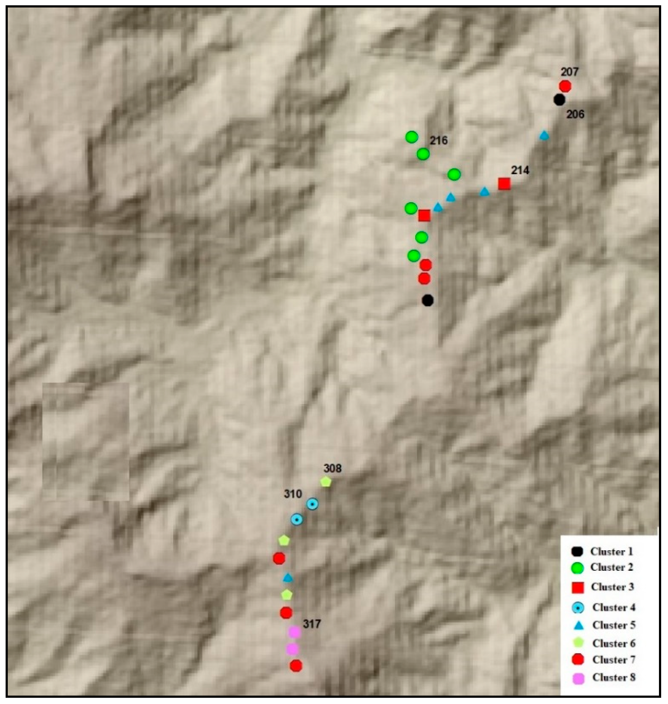
Table 4 presents the results of the cluster analysis, by having the algorithm testing from 2 up to 8 clusters. The wind farm site, due to the variability of all samplers (all variables presented a high standard deviation), showed a lower S coefficient, and only the case of 8 clusters fulfilled the criterion (S > 0.5). Figure 7 shows the clusters and Table 5 the centroid turbine of each cluster.

4.3. Neural Network Results

The network was trained with a dataset of the year 2017, splitting it with a pattern of 10 days of training and 4 days of testing, corresponding to 1440 samples of training and 576 for testing (a sample each 10 min).
The effectiveness of the data-driven model is assessed comparing the real output power of the wind farm against the output of the neural network under three different configurations:
-
All turbines: the neural network is fed with the wind direction and wind speed of all the turbines of the wind farm (28 neurons in the input layer of the neural network).
-
Random turbine: the neural network is fed with the wind direction and wind speed of a random turbine (1 neuron in the input layer of the neural network).
-
Cluster centroid: the neural network is fed with the wind direction and wind speed of the centroid turbines of the clusters (8 neurons, depending on the cluster analysis, in the input layer of the neural network)
Table 6 shows the normalized mean squared error (NMSE) retrieved for the testing dataset of 2017. The NMSE is computed using the following formula:
NMSE = 1 N i = 1 N P i P ^ i P i 2
where N is the number of samples of tests (one sample each ten minutes), P i is the real output of the wind farm of the ith sample, and P ^ i is the estimation of the network for the ith sample.
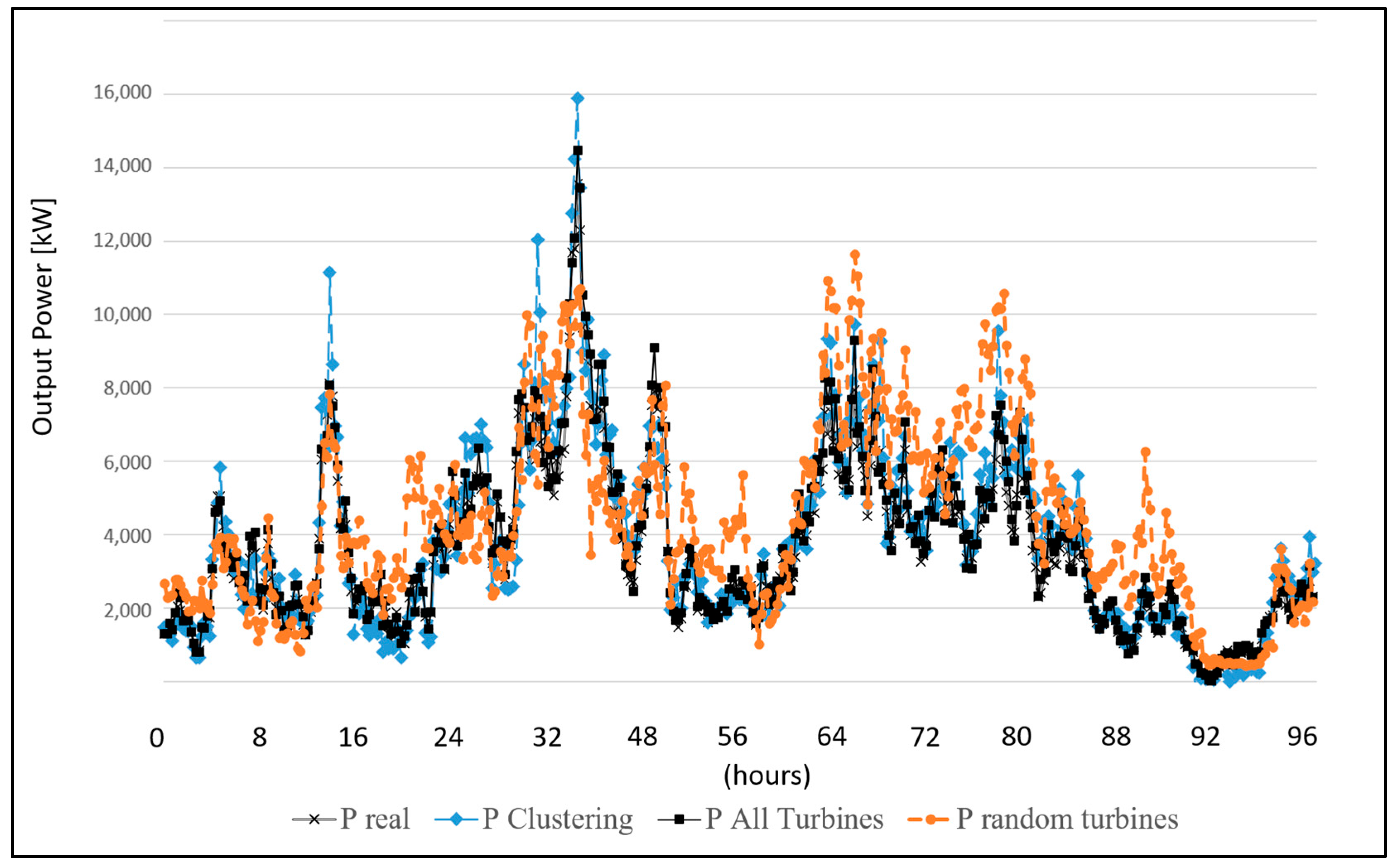
Figure 8 shows a comparison chart of these results considering a time-interval of a test of 96 h (from 10 to 14 of February 2017). From both the charts in Figure 8 and the results in Table 6, it is possible to notice that the “All Turbines” model is able to give good estimates, such that it is difficult to distinguish it from the P real trend. Nevertheless, the computing effort required to train and run the neural network is higher than the clustering model that uses only 8 input neurons against the 28 of the “All Turbines”. Finally, the random turbine model gives errors with 2 orders of magnitude higher than the “All Turbines” approach.

4.4. Hybrid Reliability Block-Diagram-Simulation Model of the Wind Turbine Generator

With the goal of improving accuracy, the data-driven model has been combined with the dependable model of failure of the wind turbine. The internal structure diagram of a wind turbine is very complex and, as discussed in [64,65], for the purpose of a dependability model they can be grouped in the subsystems shown in Table 7.
In this case study, the Hybrid Reliability Block Diagram (HBRD) used to model the wind turbine is shown in Figure 9. This approach fits with the claims of [64,65], which demonstrate that the wind speed affects the probability density function of the components of the Safety Subsystem and of the Brake Assembly. Table 7 shows the probability density functions of the subsystems used for this case study.
In the proposed model, we assume that the restoration brings back the component as good as new, with a mean time to restoration shown in Table 8.
For the HRBD proposed, the resolution is performed by implementing a Monte Carlo simulation that allows for the coding of the dynamic behavior of the reliability blocks and for integrating numerically Equations (5), (7) and (8). To this end, we require the adoption of a time-interval, Δ τ (the time-step of the simulation), which rules the discrete integration of the reliability equations. In this way it is possible to evaluate the generic working/failure state of each component by comparing the reliability at time τ with a random uniform sample value, ψ in [0, 1[. The time-step of the proposed simulation has been set to 10 min, which corresponds to the data sample of the time histories provided to train the data-driven algorithms.
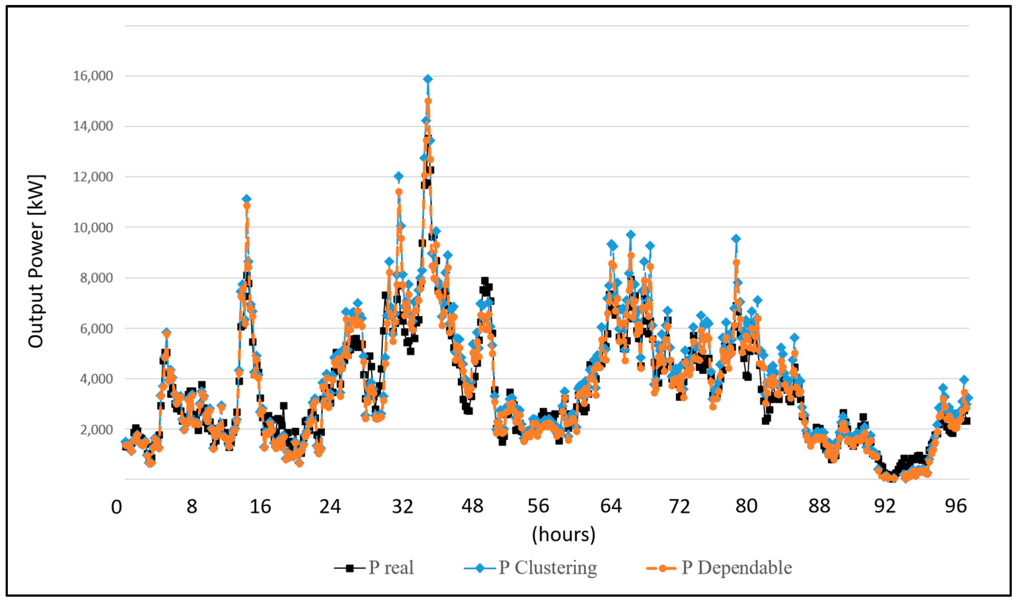
Figure 10 shows the reliability of a WTG, namely the probability that it never stops working during the mission time. In this case study, this information gives the indication that the generic WTG has roughly a probability of 78% of working continuously during the 96 h of observation. The dependability model takes as input the estimated power predicted by the data-driven model, PDD (Figure 8 and Figure 11). At each iteration of the Monte Carlo simulation it evaluates the PMC( Δ τ k ) for each Δ τ k , k = 0,…, 96 h (with a 10 min time-step), according to Equation (10):
P MC Δ τ k = 1 N i = 1 N P DD Δ τ k     WTG i   10
where N is the number of clusters and WTGi is the status of the ith centroid turbine that can be equal to 1 if the WTG is working, and 0 otherwise. To provide the status of each centroid turbine, the dependability algorithm solves the corresponding HRDB. In order to do that, each component C is evaluated by integrating the corresponding failure rate (see Equations (6)–(8)) and comparing it with a random uniform value, ρ ∈ in [0, 1[, sampled at each time-step, according to the logic of Equation (11):
Φ Δ τ k = OK ,   if   rand > R Δ τ k KO ,   if   rand R Δ τ k  
If the component C has failed, the dependability algorithm samples the next repair time using the inverse function of the repair distribution. More details can be found in [67].
The Monte Carlo simulation of the HRBD has been set to run 104 iterations, and Figure 11 shows the charts comparing the improvement in the dependable model with respect to the clustering (this figure also presents the prediction of the days from 10 to 14 February 2017). In Table 9, the comparison of the normalized mean squared error of the power output between the clustering and the dependable algorithms are shown.
It is possible to notice that the dependable model retrieves a more accurate evaluation compared to the Pcluster algorithm. This result is clearer if we consider the prediction of the energy produced as shown in Figure 12. This value can be obtained during the same 96 h of observation with the formula of Equation (12):
E PRED = i = 1 N P i
where N is the number of samples and Pi is the output power of the wind farm for the ith sample.
Table 10 displays the normalized mean squared error values for the estimated energy of the testing dataset, comparing two models: the dependable model and the model based solely on clustering. The results clearly demonstrate the advantage of incorporating dependability models into the energy estimation process for wind farms. By doing so, the methodology not only achieves higher accuracy in predicting energy production, but also offers insights into the operational efficiency and potential output of wind farms under varying conditions.

4.5. Results Discussion

The need to improve the accuracy of the solo data-driven clustering algorithm has motivated the idea of coupling it with a dependable model also, as proposed in previous research [31], where this solution was tested for long-term production estimation of a analytical wake model. These two approaches are thus not comparable in terms of results.
Compared with existing material [11,15,28,32,34,37,49], the proposed approach introduces several novel aspects that collectively advance the subject area. First, analyzing other similar research papers that adopt a data-driven model with an ANN, it is possible to highlight the fact that none of those make use of a dependable model of the wind turbine.
As far as the data-driven model based on ANN is concerned, the efficient use of data through centroid turbines offers a novel way of reducing computational demands by focusing on ‘centroid turbines’ for data collection and analysis. This strategy, underexplored in the literature [15,17,18,19,20], optimizes the forecasting process by minimizing the data required without compromising the accuracy of the output. It provides a practical solution to the challenges of data management in large wind farms, setting a new direction for future research in the area. In this way, the methodology presented addresses the common trade-off between computational load and prediction accuracy, tackled by different literature studies with other regression algorithms [11,15,29,38,40,45,51], maintaining high precision in forecasts while reducing computational effort. Beyond theoretical advancements, this study has practical implications for wind farm management, as it helps in simplifying the site assessment phase and it enhances real-time operational decision-making, suggesting ways to reduce costs and improve efficiency in wind energy production.
The experimental campaign of the wind farm case study reveals that the dependable model proposed significantly outperforms the solo-clustering model. Specifically, for the year 2017, the total NMSE for the dependable model (NMSE_dependable) is 0.00905, in contrast to 0.04344 for the clustering model (NMSE_clustering). This difference indicates a substantial improvement in accuracy, with the dependable model being approximately 4.8 times more accurate than the clustering model, which equates to a 480% increase in accuracy.

5. Conclusions

In this study, a novel methodology for the short-term estimation of wind farm output has been introduced. The proposed methodology integrates an artificial intelligence framework with a data-driven approach alongside a stochastic model assessing wind turbine generator reliability. At the heart of the approach is the use of a multilayer perceptron (MLP) neural network, which undergoes training and evaluation over dataset patterns spanning 10 days for training and 4 days for testing. The findings indicate that through clustering analysis, it is possible to significantly reduce the number of input neurons required in the neural network without compromising the accuracy of power output predictions. This reduction presents substantial benefits in two key areas. Firstly, it simplifies the process of assessing wind farm productivity potential during the site selection phase. Specifically, engineers may not need to deploy as many anemometers as initially anticipated, correlating directly with the reduced number of critical wind turbines (centroid turbines of clusters) identified through clustering. This not only streamlines the preliminary engineering work, but also can lead to cost savings in the equipment and labor required for site analysis. Secondly, for real-time operational scenarios, the proposed methodology offers the advantage of reduced computational demands. By needing to process information from fewer input neurons, the system can generate short-term productivity estimates more efficiently. This efficiency is particularly beneficial in scenarios where rapid decision-making is critical, enhancing operational responsiveness and potentially reducing the computational resources required for data processing and analysis. Together, these advantages demonstrate the utility of the proposed approach in both the planning and operational phases of wind farm management, offering a means to optimize both the initial site assessment and ongoing power output estimation with a focus on computational efficiency and practicality.
The impact of the clustering approach has been demonstrated in the first part of the experimental section. When the neural network is trained and used with the turbines identified by cluster analysis (8 turbines), the normalized mean squared error (NMSE) values increase in comparison to the full data set (28 turbines), yet they are still within a reasonable range. This increase implies a reduction in prediction accuracy, which is expected due to the decreased number of input variables. However, the relatively low NMSE (compared to the random turbine selection) suggests that the clustering method is effective in identifying representative turbines that still enable the neural network to make relatively accurate predictions, albeit with reduced computational effort.
The integration of a Hybrid Reliability Block Diagram (HRBD) model marks a significant advancement in refining the accuracy of the estimations, being able to incorporate the variability in operational conditions of wind turbines over time. The second part of the experimental section shows the benefit of such coupling. Results demonstrated that the reliability model furnishes a more precise evaluation of energy production, particularly over short-term periods, when compared to results obtained solely from the clustering algorithm. These outcomes strongly indicate that a synergistic approach, combining both clustering techniques and stochastic reliability models, can substantially improve the accuracy and dependability of predictions for wind power plant energy output.
While the methodology proposed in this study demonstrates a good capability for predicting the production of the wind farm through neural networks and clustering algorithms, it is important to acknowledge a pivotal limitation: the reliance on accurate and timely wind speed and direction forecasts. In fact, for the neural network to provide precise estimations, it requires wind forecasts for the upcoming interval of time for which the prediction is requested. This dependency underscores a crucial challenge; although acquiring short-term wind forecasts is a common practice within the wind power industry for operational planning, grid integration, and maintenance scheduling, the accuracy of these forecasts can vary, especially as the forecast period extends. This highlights a potential constraint in real-time operation and maintenance scenarios, where the quality of forecasts directly impacts the precision of power production estimates. Thus, while this approach offers a streamlined and efficient method for estimating wind power production, the accuracy of these estimations is fundamentally tied to the availability and precision of short-term wind forecasts.
In conclusion, this study presents a refined approach to estimating wind power production, demonstrating slight but significant improvements in precision by integrating a neural network with a dependability model. This enhancement is contingent upon a thorough understanding of wind turbine failure rates and fault behaviors, which are critical inputs for the dependability model. Accurately incorporating these factors is essential for realizing the full potential of the methodology in improving prediction accuracy.
Future research will focus on optimizing the dependability model by enhancing its adaptability to diverse operational conditions and maintenance schedules. Additionally, we aim to explore the integration of advanced weather forecasting techniques to further refine our predictions. These focused areas of study promise to elevate the efficiency and reliability of wind power forecasting, contributing to the broader goal of advancing renewable energy technologies.
By addressing these specific aspects, we not only aim to bolster the methodology’s robustness, but also to ensure its applicability in the dynamic landscape of wind energy production. The importance of production estimation in renewable energy cannot be overstated. Its multifaceted impact on planning, integration, operational efficiency, investment decisions, and cost reduction underscores its role as a cornerstone in the transition towards a stable, efficient, and economically viable renewable energy landscape.
Up until now, the proposed methodology has held promise for advancing the accuracy and reliability of short-term wind power predictions, contributing to the efficient integration of wind energy into the electricity grid.

Author Contributions

F.F.: conceptualization, methodology, investigation, software, writing—original draft, writing—review and editing; S.B.: resources, methodology, supervision; F.C.: methodology, investigation, software, writing—original draft, writing—review and editing; L.M.O.: data curation, visualization, writing—original draft, writing—review and editing. All authors have read and agreed to the published version of the manuscript.

Funding

This research received no external funding.

Data Availability Statement

The data presented in this study are available on request from the corresponding author. The data are not publicly available due to privacy.

Conflicts of Interest

The authors declare no conflicts of interest.

Abbreviations

AcronymDefinition
ANN Artificial Neural Network
IPCC Intergovernmental Panel for Climate Change
GWECGlobal Wind Energy Council
MLP Multilayer Perceptron
AIArtificial Intelligence
ANNsArtificial Neural Networks
SVMsSupport Vector Machines
SVRSupport Vector Regression
GPR Gaussian Process Regression
BS Bootstrap
PIs Prediction Intervals
NWP Numerical Weather Prediction
ARIMA Autoregressive Integrated Moving Average
NARX Non-Linear Autoregressive Network with exogenous inputs
VMDVariational Mode Decomposition
MRMRMaximum Relevance and Minimum Redundancy Algorithm
LSTMLong Short-Term Memory Neural Network
FA Firefly Algorithm
kNN K-Nearest Neighbor
GP Gaussian Process
VMDVariational Mode Decomposition
TCN Temporal Convolutional Network Model
SIA Seasonal Index Adjustment
ERNN Elman Recurrent Neural Network
FMOGMDRPs Flexibility-based Multi-Objective Generation Maintenance scheduling associated with Demand Response Programs
PSO Particle Swarm Optimization
GIS Geographic Information System
SCADASupervisory Control And Data Acquisition
DCSDistributed Control System
RBDs Reliability Block Diagrams
HBRD Hybrid Reliability Block Diagram
SHyFTOO Stochastic Hybrid Fault Tree Object Oriented
NMSE normalized mean squared error
PDFProbability density function

References

  1. Horowitz, C.A. Paris Agreement. Int. Leg. Mater. 2016, 55, 740–755. [Google Scholar] [CrossRef]
  2. EU Commission. Regulation (EU) 2021/1119 of the European Parliament and of the Council of 30 June 2021 Establishing the Framework for Achieving Climate Neutrality; The European Parliament and the Council of The European Union: Brussels, Belgium, 2021. [Google Scholar]
  3. European Commission. REPowerEU: Joint European Action for More Affordable, Secure and Sustainable Energy. Communication from the Commission to the European Parliament, the European Council, the Council, the European Economic and Social Committee and the Committee of the Regions. Strasbourg, 8 March 2022, COM (2022) 108 Final. 2022. Available online: https://eur-lex.europa.eu/legal-content/EN/TXT/?uri=celex:52022DC0108 (accessed on 11 December 2023).
  4. European Commission. Communication from the Commission to the European Parliament, the European Council, the European Economic and Social Committee and the Committee of the Regions. The European Green Deal. Brussels, 11 December 2019, COM (2019) 640 Final. Available online: https://eur-lex.europa.eu/legal-content/EN/TXT/?uri=COM%3A2019%3A640%3AFIN (accessed on 11 December 2023).
  5. GWEC–Global Wind Energy Council. GWEC–Global Wind Report 2023. Available online: https://gwec.net/globalwindreport2023/ (accessed on 19 March 2024).
  6. Cacciuttolo, C.; Cano, D.; Guardia, X.; Villicaña, E. Renewable Energy from Wind Farm Power Plants in Peru: Recent Advances, Challenges, and Future Perspectives. Sustainability 2024, 16, 1589. [Google Scholar] [CrossRef]
  7. Fan, Q.; Wang, X.; Yuan, J.; Liu, X.; Hu, H.; Lin, P. A Review of the Development of Key Technologies for Offshore Wind Power in China. J. Mar. Sci. Eng. 2022, 10, 929. [Google Scholar] [CrossRef]
  8. Yan, J.; Liu, Y.; Han, S.; Wang, Y.; Feng, S. Reviews on Uncertainty Analysis of Wind Power Forecasting. Renew. Sustain. Energy Rev. 2015, 52, 1322–1330. [Google Scholar] [CrossRef]
  9. Hodge, B.M.; Milligan, M. Wind Power Forecasting Error Distributions over Multiple Timescales. In Proceedings of the IEEE Power and Energy Society General Meeting, Detroit, MI, USA, 24–28 July 2011. [Google Scholar]
  10. Chang, G.W.; Lu, H.J.; Chang, Y.R.; Lee, Y.D. An Improved Neural Network-Based Approach for Short-Term Wind Speed and Power Forecast. Renew. Energy 2017, 105, 301–311. [Google Scholar] [CrossRef]
  11. Wang, J.; Qin, S.; Zhou, Q.; Jiang, H. Medium-Term Wind Speeds Forecasting Utilizing Hybrid Models for Three Different Sites in Xinjiang, China. Renew. Energy 2015, 76, 91–101. [Google Scholar] [CrossRef]
  12. Kirchner-Bossi, N.; García-Herrera, R.; Prieto, L.; Trigo, R.M. A Long-Term Perspective of Wind Power Output Variability. Int. J. Climatol. 2015, 35, 2635–2646. [Google Scholar] [CrossRef]
  13. Landberg, L. A mathematical look at a physical power prediction model. Wind Energy Int. J. Prog. Appl. Wind Power Convers. Technol. 1998, 1, 23–28. [Google Scholar] [CrossRef]
  14. Landberg, L.; Myllerup, L.; Rathmann, O.; Petersen, E.L.; Jørgensen, B.H.; Badger, J.; Mortensen, N.G. Wind Resource Estimation–An Overview. Wind Energy 2003, 6, 261–271. [Google Scholar] [CrossRef]
  15. Kavasseri, R.G.; Seetharaman, K. Day-Ahead Wind Speed Forecasting Using f-ARIMA Models. Renew. Energy 2009, 34, 1388–1393. [Google Scholar] [CrossRef]
  16. Carolin Mabel, M.; Fernandez, E. Analysis of Wind Power Generation and Prediction Using ANN: A Case Study. Renew. Energy 2008, 33, 986–992. [Google Scholar] [CrossRef]
  17. Giebel, G.; Brownsword, R.; Kariniotakis, G.; Denhard, M.; Draxl, C. The State of the Art in Short-Term Prediction of Wind Power, A Literature Overview; ANEMOS.plus. 2011. Available online: https://orbit.dtu.dk/en/publications/the-state-of-the-art-in-short-term-prediction-of-wind-power-a-lit (accessed on 7 March 2024).
  18. Hao, Y.; Wang, Q.; Ma, T.; Du, J.; Cao, J. Energy Allocation and Task Scheduling in Edge Devices Based on Forecast Solar Energy with Meteorological Information. J. Parallel Distrib. Comput. 2023, 177, 171–181. [Google Scholar] [CrossRef]
  19. Sharifi, V.; Abdollahi, A.; Rashidinejad, M. Flexibility-Based Generation Maintenance Scheduling in Presence of Uncertain Wind Power Plants Forecasted by Deep Learning Considering Demand Response Programs Portfolio. Int. J. Electr. Power Energy Syst. 2022, 141, 108225. [Google Scholar] [CrossRef]
  20. Ying, C.; Wang, W.; Yu, J.; Li, Q.; Yu, D.; Liu, J. Deep Learning for Renewable Energy Forecasting: A Taxonomy, and Systematic Literature Review. J. Clean. Prod. 2023, 384, 135414. [Google Scholar] [CrossRef]
  21. Notton, G.; Nivet, M.L.; Voyant, C.; Paoli, C.; Darras, C.; Motte, F.; Fouilloy, A. Intermittent and Stochastic Character of Renewable Energy Sources: Consequences, Cost of Intermittence and Benefit of Forecasting. Renew. Sustain. Energy Rev. 2018, 87, 96–105. [Google Scholar] [CrossRef]
  22. Way, R.; Ives, M.C.; Mealy, P.; Farmer, J.D. Empirically Grounded Technology Forecasts and the Energy Transition. Joule 2022, 6, 2057–2082. [Google Scholar] [CrossRef]
  23. Lee, J.C.Y.; Jason Fields, M. An Overview of Wind-Energy-Production Prediction Bias, Losses, and Uncertainties. Wind Energy Sci. 2021, 6, 311–365. [Google Scholar] [CrossRef]
  24. Costa, A.; Crespo, A.; Navarro, J.; Lizcano, G.; Madsen, H.; Feitosa, E. A Review on the Young History of the Wind Power Short-Term Prediction. Renew. Sustain. Energy Rev. 2008, 12, 1725–1744. [Google Scholar] [CrossRef]
  25. Ernst, B.; Reyer, F.; Vanzetta, J. Wind Power and Photovoltaic Prediction Tools for Balancing and Grid Operation. In Proceedings of the 2009 CIGRE/IEEE PES Joint Symposium: Integration of Wide-Scale Renewable Resources into the Power Delivery System, Calgary, AB, Canada, 29–31 July 2009. [Google Scholar]
  26. Soman, S.S.; Zareipour, H.; Malik, O.; Mandal, P. A Review of Wind Power and Wind Speed Forecasting Methods with Different Time Horizons. In Proceedings of the North American Power Symposium 2010, NAPS 2010, Arlington, TX, USA, 26–28 September 2010. [Google Scholar]
  27. Li, C.; Lin, S.; Xu, F.; Liu, D.; Liu, J. Short-Term Wind Power Prediction Based on Data Mining Technology and Improved Support Vector Machine Method: A Case Study in Northwest China. J. Clean. Prod. 2018, 205, 909–922. [Google Scholar] [CrossRef]
  28. Lange, M.; Focken, U. Physical Approach to Short-Term Wind Power Prediction; Springer: Berlin/Heidelberg, Germany, 2006. [Google Scholar]
  29. Najeebullah; Zameer, A.; Khan, A.; Javed, S.G. Machine Learning Based Short Term Wind Power Prediction Using a Hybrid Learning Model. Comput. Electr. Eng. 2015, 45, 122–133. [Google Scholar] [CrossRef]
  30. Li, H.; Jiang, Z.; Shi, Z.; Han, Y.; Yu, C.; Mi, X. Wind-Speed Prediction Model Based on Variational Mode Decomposition, Temporal Convolutional Network, and Sequential Triplet Loss. Sustain. Energy Technol. Assess. 2022, 52, 101980. [Google Scholar] [CrossRef]
  31. Famoso, F.; Brusca, S.; D’Urso, D.; Galvagno, A.; Chiacchio, F. A Novel Hybrid Model for the Estimation of Energy Conversion in a Wind Farm Combining Wake Effects and Stochastic Dependability. Appl. Energy 2020, 280, 115967. [Google Scholar] [CrossRef]
  32. Ioakimidis, C.S.; Genikomsakis, K.N.; Dallas, P.I.; Lopez, S. Short-Term Wind Speed Forecasting Model Based on ANN with Statistical Feature Parameters. In Proceedings of the IECON 2015–41st Annual Conference of the IEEE Industrial Electronics Society, Yokohama, Japan, 9–12 November 2015. [Google Scholar]
  33. Rahman, M.M.; Shakeri, M.; Tiong, S.K.; Khatun, F.; Amin, N.; Pasupuleti, J.; Hasan, M.K. Prospective Methodologies in Hybrid Renewable Energy Systems for Energy Prediction Using Artificial Neural Networks. Sustainability 2021, 13, 2393. [Google Scholar] [CrossRef]
  34. Tascikaraoglu, A.; Uzunoglu, M. A Review of Combined Approaches for Prediction of Short-Term Wind Speed and Power. Renew. Sustain. Energy Rev. 2014, 34, 243–254. [Google Scholar] [CrossRef]
  35. Thordarson, F.Ö.; Madsen, H.; Nielsen, H.A.; Pinson, P. Conditional Weighted Combination of Wind Power Forecasts. Wind Energy 2010, 13, 751–763. [Google Scholar] [CrossRef]
  36. Foley, A.M.; Leahy, P.G.; Marvuglia, A.; McKeogh, E.J. Current Methods and Advances in Forecasting of Wind Power Generation. Renew. Energy 2012, 37, 1–8. [Google Scholar] [CrossRef]
  37. Ramasamy, P.; Chandel, S.S.; Yadav, A.K. Wind Speed Prediction in the Mountainous Region of India Using an Artificial Neural Network Model. Renew. Energy 2015, 80, 338–347. [Google Scholar] [CrossRef]
  38. Sharifzadeh, M.; Sikinioti-Lock, A.; Shah, N. Machine-Learning Methods for Integrated Renewable Power Generation: A Comparative Study of Artificial Neural Networks, Support Vector Regression, and Gaussian Process Regression. Renew. Sustain. Energy Rev. 2019, 108, 513–538. [Google Scholar] [CrossRef]
  39. Jursa, R.; Rohrig, K. Short-Term Wind Power Forecasting Using Evolutionary Algorithms for the Automated Specification of Artificial Intelligence Models. Int. J. Forecast. 2008, 24, 694–709. [Google Scholar] [CrossRef]
  40. Di Piazza, A.; Di Piazza, M.C.; La Tona, G.; Luna, M. An Artificial Neural Network-Based Forecasting Model of Energy-Related Time Series for Electrical Grid Management. Math. Comput. Simul. 2021, 184, 294–305. [Google Scholar] [CrossRef]
  41. Qin, G.; Yan, Q.; Zhu, J.; Xu, C.; Kammen, D.M. Day-Ahead Wind Power Forecasting Based on Wind Load Data Using Hybrid Optimization Algorithm. Sustainability 2021, 13, 1164. [Google Scholar] [CrossRef]
  42. Li, L.L.; Zhao, X.; Tseng, M.L.; Tan, R.R. Short-Term Wind Power Forecasting Based on Support Vector Machine with Improved Dragonfly Algorithm. J. Clean. Prod. 2020, 242, 118447. [Google Scholar] [CrossRef]
  43. Yesilbudak, M.; Sagiroglu, S.; Colak, I. A Novel Implementation of KNN Classifier Based on Multi-Tupled Meteorological Input Data for Wind Power Prediction. Energy Convers. Manag. 2017, 135, 434–444. [Google Scholar] [CrossRef]
  44. Treiber, N.A.; Kramer, O. Evolutionary Feature Weighting for Wind Power Prediction with Nearest Neighbor Regression. In Proceedings of the 2015 IEEE Congress on Evolutionary Computation, CEC 2015-Proceedings, Sendai, Japan, 25–28 May 2015. [Google Scholar]
  45. Kramer, O.; Gieseke, F. Short-Term Wind Energy Forecasting Using Support Vector Regression. In Proceedings of the Soft Computing Models in Industrial and Environmental Applications, 6th International Conference SOCO 2011, Salamanca, Spain, 6–8 April 2011; Advances in Intelligent and Soft Computing. Springer: Berlin/Heidelberg, Germany, 2011; Volume 87. [Google Scholar]
  46. Chen, N.; Qian, Z.; Nabney, I.T.; Meng, X. Wind Power Forecasts Using Gaussian Processes and Numerical Weather Prediction. IEEE Trans. Power Syst. 2014, 29, 656–665. [Google Scholar] [CrossRef]
  47. D’Urso, D.; Chiacchio, F.; Cavalieri, S.; Gambadoro, S.; Khodayee, S.M. Predictive Maintenance of Standalone Steel Industrial Components Powered by a Dynamic Reliability Digital Twin Model with Artificial Intelligence. Reliab. Eng. Syst. Saf. 2024, 243, 109859. [Google Scholar] [CrossRef]
  48. Sánchez, I. Short-Term Prediction of Wind Energy Production. Int. J. Forecast. 2006, 22, 43–56. [Google Scholar] [CrossRef]
  49. Al-Dahidi, S.; Baraldi, P.; Zio, E.; Lorenzo, M. Bootstrapped Ensemble of Artificial Neural Networks Technique for Quantifying Uncertainty in Prediction of Wind Energy Production. Sustainability 2021, 13, 6417. [Google Scholar] [CrossRef]
  50. Cassola, F.; Burlando, M. Wind Speed and Wind Energy Forecast through Kalman Filtering of Numerical Weather Prediction Model Output. Appl. Energy 2012, 99, 154–166. [Google Scholar] [CrossRef]
  51. Wang, Y.; Wang, D.; Tang, Y. Clustered Hybrid Wind Power Prediction Model Based on ARMA, PSO-SVM, and Clustering Methods. IEEE Access 2020, 8, 17071–17079. [Google Scholar] [CrossRef]
  52. Cox, J. Impact of Intermittency: How Wind Variability Could Change the Shape of the British and Irish Electricity Markets; Poyry Energy (Oxford) Ltd.: Oxford, UK, 2009. [Google Scholar]
  53. Sinden, G. Characteristics of the UK Wind Resource: Long-Term Patterns and Relationship to Electricity Demand. Energy Policy 2007, 35, 112–127. [Google Scholar] [CrossRef]
  54. Kubik, M.L.; Coker, P.J.; Barlow, J.F.; Hunt, C. A Study into the Accuracy of Using Meteorological Wind Data to Estimate Turbine Generation Output. Renew. Energy 2013, 51, 153–158. [Google Scholar] [CrossRef]
  55. Wang, P.; Li, Y.; Zhang, G. Probabilistic Power Curve Estimation Based on Meteorological Factors and Density LSTM. Energy 2023, 269, 126768. [Google Scholar] [CrossRef]
  56. Berghout, T.; Benbouzid, M.; Amirat, Y. Interaction between Machine Learning and Maintenance Planning for Wind Energy Systems: A Theoretical Review and Analysis. In Proceedings of the 2023 IEEE 2nd Industrial Electronics Society Annual On-Line Conference (ONCON), Online Conference, 8–10 December 2023; IEEE: Piscataway, NJ, USA, 2023; pp. 1–6. [Google Scholar]
  57. Brusca, S.; Famoso, F.; Lanzafame, R.; Galvagno, A.; Mauro, S.; Messina, M. Wind Farm Power Forecasting: New Algorithms with Simplified Mathematical Structure. AIP Conf. Proc. 2019, 2191, 020028. [Google Scholar]
  58. Spinato, F.; Tavner, P.J.; Van Bussel, G.J.W.; Koutoulakos, E. Reliability of Wind Turbine Subassemblies. IET Renew. Power Gener. 2009, 3, 387–401. [Google Scholar] [CrossRef]
  59. Wang, S.; Tomovic, M.; Liu, H. Comprehensive Reliability Design of Aircraft Hydraulic System. In Commercial Aircraft Hydraulic Systems; Shanghai Jiao Tong University Press: Shanghai, China, 2016. [Google Scholar]
  60. Brusca, S.; Lanzafame, R.; Famoso, F.; Galvagno, A.; Messina, M.; Mauro, S.; Prestipino, M. On the Wind Turbine Wake Mathematical Modelling. Energy Procedia 2018, 148, 202–209. [Google Scholar] [CrossRef]
  61. Faulstich, S.; Hahn, B.; Tavner, P.J. Wind Turbine Downtime and Its Importance for Offshore Deployment. Wind Energy 2011, 14, 327–337. [Google Scholar] [CrossRef]
  62. Qiao, W.; Lu, D. A Survey on Wind Turbine Condition Monitoring and Fault Diagnosis—Part I: Components and Subsystems. IEEE Trans. Ind. Electron. 2015, 62, 6536–6545. [Google Scholar] [CrossRef]
  63. Pfaffel, S.; Faulstich, S.; Rohrig, K. Performance and Reliability of Wind Turbines: A Review. Energies 2017, 10, 1904. [Google Scholar] [CrossRef]
  64. Khodayee, S.M.; Oliveri, L.; Aizpurua, J.I.; D’Urso, D.; Chiacchio, F. Reliability Simulation of a Multi-State Wind Turbine Generator Using SHyFTOO. In Proceedings of the 21st International Conference on Modeling and Applied Simulation, MAS 2022, Rome, Italy, 19–21 September 2022. [Google Scholar]
  65. Su, C.; Fu, Y.Q. Reliability Assessment for Wind Turbines Considering the Influence of Wind Speed Using Bayesian Network. Eksploat. Niezawodn. 2014, 16, 1–8. [Google Scholar]
  66. Bilendo, F.; Meyer, A.; Badihi, H.; Lu, N.; Cambron, P.; Jiang, B. Applications and Modeling Techniques of Wind Turbine Power Curve for Wind Farms—A Review. Energies 2023, 16, 180. [Google Scholar] [CrossRef]
  67. Chiacchio, F.; Aizpurua, J.I.; Compagno, L.; D’Urso, D. SHyFTOO, an Object-Oriented Monte Carlo Simulation Library for the Modeling of Stochastic Hybrid Fault Tree Automaton. Expert Syst. Appl. 2020, 146, 113139. [Google Scholar] [CrossRef]
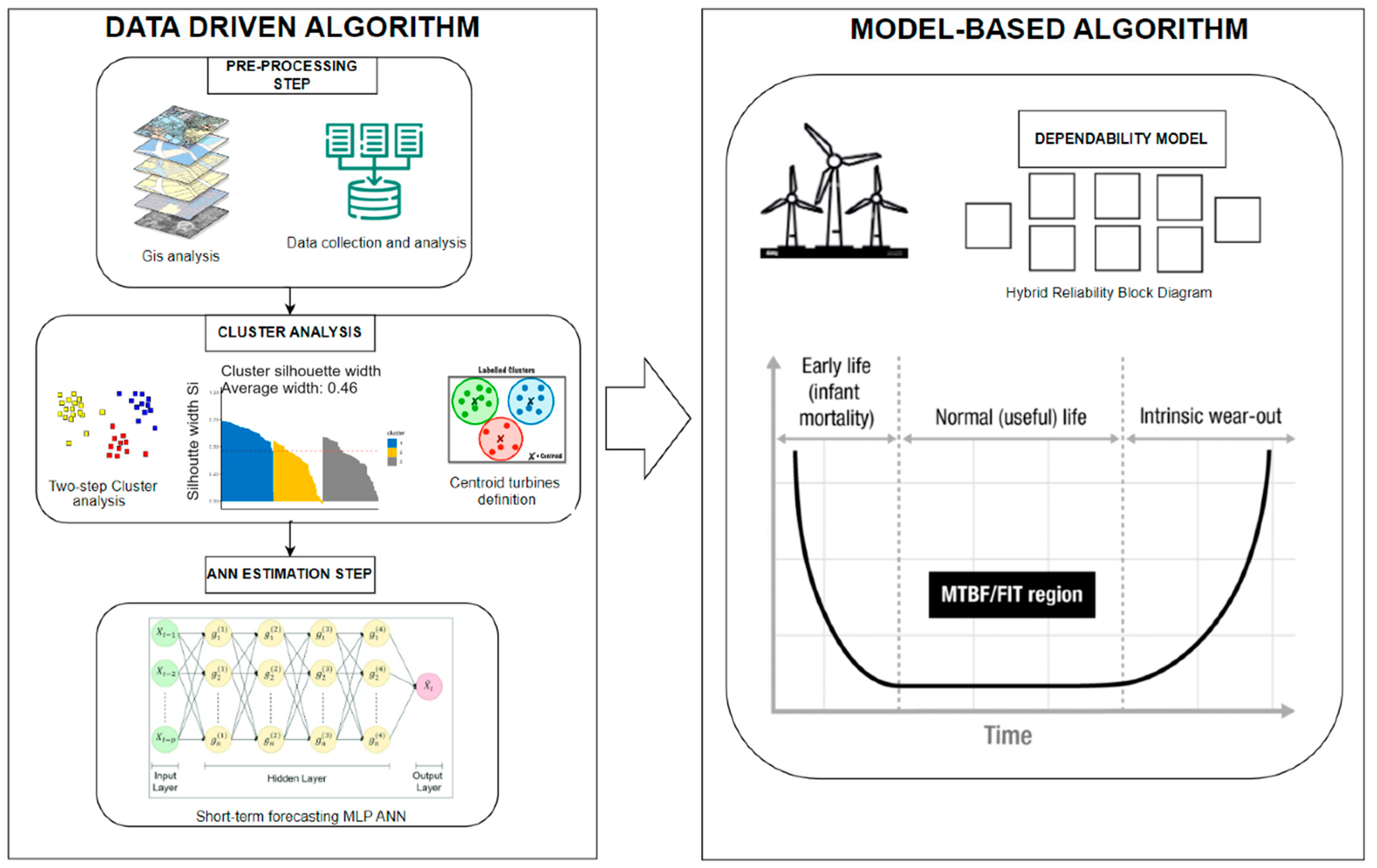
Figure 1. Steps of the hybrid algorithm for the short-term energy estimation.
Energies 17 01627 g001
Figure 3. Example of Reliability Block Diagram.
Energies 17 01627 g003
Figure 4. The power curve of the turbine model for an air density of 1.225 kg/m3 [57].
Energies 17 01627 g004
Figure 5. Locations of the 28 turbines of the wind farm.
Energies 17 01627 g005
Figure 6. The distribution of the wind directions for 8 turbines (1 per cluster) [57].
Energies 17 01627 g006
Figure 7. The geographical cluster distribution of the wind farm.
Energies 17 01627 g007
Figure 8. The real and estimated power (96 h, 10 to 14 of February 2017).
Energies 17 01627 g008
Figure 9. Hybrid Reliability Block Diagram of the wind turbine generator.
Energies 17 01627 g009
Figure 10. Reliability of the generic WTG in 96 h of continuous activity.
Energies 17 01627 g010
Figure 11. Comparison among real, clustering and dependable power predictions (96 h, 10 to 14 of February 2017).
Energies 17 01627 g011
Figure 12. The real, the cluster and the dependable prediction energy during the 96 h.
Energies 17 01627 g012
Table 1. Classification of Papers by Approach and Model used.
ApproachModel UsedReference
Number
Data-DrivenAutoregressive Integrated Moving Mean Models (ARIMA)[15]
Artificial neural networks (ANNs)[32,34,37,49]
Artificial neural networks (ANNs), Support Vector Regression (SVR), Gaussian Process Regression (GPR)[38]
Evolutionary Optimization Algorithms, Neural Networks, Nearest Neighbor Search[39]
Non-Linear Autoregressive Network with Exogenous Inputs (NARX) ANN[40]
Variational Mode Decomposition (VMD), Maximum Relevance and Minimum Redundancy Algorithm (MRMR), Long Short-Term Memory Neural Network (LSTM), Firefly Algorithm (FA)[41]
Support Vector Machines (SVMs)[42]
K-Nearest Neighbor Classifier (kNN)[43,44]
Support Vector Regression (SVR)[45]
Gaussian Process (GP), Numerical Weather Prediction Model (NWP) [46]
Statistical Forecasting System[48]
Kalman Filters[50]
Model-BasedAtmospheric Fluid Dynamics[13,28]
Variational Mode Decomposition (VMD), Temporal Convolutional Network Model (TCN) [30]
Jensen wake mathematical theory[31]
HybridSupport Vector Regression (SVR), Seasonal Index Adjustment (SIA) and Elman Recurrent Neural Network (ERNN)[11]
Non-dominated Sorting Genetic Algorithms[18]
Flexibility-based Multi-Objective Generation Maintenance scheduling associated with Demand Response Programs (FMOGMDRPs)[19]
Support Vector Machine (SVM) and Data Mining[27]
Machine-Learning based Short-Term Wind Power Prediction and Support Vector Regression[29]
Conditional Weighted Combination Method[35]
Dynamic Reliability Digital Twin[47]
AutoRegressive Moving Average (ARMA), Support Vector Machine (SVM), Particle Swarm Optimization (PSO)[51]
Table 2. Main characteristics of the wind farm.
FeatureSite
Position37°58′32″ N, 15°07′00″ E
N° Turbines28
Turbine quote732–1149 m
Turbine Height52–58 m
N° Blades3
Turbine Pout850 kW
Table 3. Main data of statistical variables (second week of February 2017) [57].
Turbine IDMean Pout [kW]Max Pout [kW]Dev.std Pout [kW]Mean Wind Speed [m/s]Max
Wind Speed [m/s]
Dev.std
Wind Speed [m/s]
206163.75850199.615.6723.713.27
21675.89828.73146.394.0716.212.38
214351.51843.11194.187.7121.453.48
309144.21848.55198.835.8520.353.53
213170.69849.81206.235.5727.763.30
308216.21849.99229.906.5125.173.59
207163.88848.45204.535.2133.813.47
317111.42849.41165.924.8517.862.54
Table 4. Silhouette results.
Cluster Silhouette Results
2345678
Coef. Silh.0.4230.4450.4670.4720.4850.4950.511
Table 5. The centroid turbines of the cluster analysis.
ClustersTurbine IDCentroid Turbine ID
Cluster 1206, 226206
Cluster 2216, 217, 220, 222, 223216
Cluster 3214, 221214
Cluster 4309, 310309
Cluster 5210, 213, 318, 219, 313213
Cluster 6308, 311, 314,308
Cluster 7207, 224, 225, 312, 315,318207
Cluster 8316, 317317
Table 6. Comparison of the Normalized Mean Squared Error of the power output.
MonthNMSE_All TurbinesNMSE_ClusteringNMSE_Random Turbine
January0.019450.696486.81375
February0.021260.658396.66039
March0.019350.659676.49241
April0.020750.767126.28689
May0.023030.661726.82694
June0.021710.755466.12375
July0.020950.685176.64920
August0.020170.760306.68725
September0.022130.750236.45569
October0.022650.716576.17180
November0.023210.774366.37107
December0.022230.722786.33632
Table 7. Probability density function (PDF) of the components of the Safety Subsystem and of the Brake Assembly.
Component
ID
DescriptionPDF
(0 < wspd ≤ 20)
PDF
(wspd > 20)
C1GeneratorWeibull (76,000; 1.2)Weibull (76,000; 1.2)
C2GearboxWeibull (123,000; 1.05)Weibull (123,000; 1.05)
C3BladeNormal (42,000; 663)Normal (42,000; 663)
C4Electrical SystemWeibull (35,000; 1.5)Weibull (35,000; 1.5)
C5Converter SystemExponential (1/45,000)Exponential (1/45,000)
H6Pitch AssemblyNormal (84,534; 506)Normal (14,089; 506)
H7Yaw AssemblyExponential (1/65,000)Exponential (1/8125)
H8Hydraulic AssemblyWeibull (66,000; 1.3)Weibull (33,000; 1.3)
H9Air BrakeExponential (1/100,000)Exponential (9/500,000)
H10Mechanical BrakeExponential (1/120,000)Exponential (1/30,000)
Table 8. Mean time to restoration with an exponential probability density function.
Component
ID
DescriptionPDF
(0 < wspd ≤ 20)
C1GeneratorExponential (1/120,000)
C2GearboxExponential (1/120,000)
C3BladeExponential (1/120,000)
C4Electrical SystemExponential (1/120,000)
C5Converter SystemExponential (1/45,000)
H6Pitch AssemblyExponential (1/120,000)
H7Yaw AssemblyExponential (1/120,000)
H8Hydraulic AssemblyExponential (1/120,000)
H9Air BrakeExponential (1/100,000)
H10Mechanical BrakeExponential (1/120,000)
Table 9. Comparison of NMSE of the power output between dependable and clustering approach.
MonthNMSE_DependableNMSE_Clustering
January0.530270.69648
February0.545530.65839
March0.516230.65967
April0.536060.76712
May0.512030.66172
June0.531970.75546
July0.534210.68517
August0.544460.76030
September0.531520.75023
October0.523610.71657
November0.538110.77436
December0.534720.72278
Table 10. Normalized Mean Squared Error of the energy produced.
MonthNMSE_DependableNMSE_Clustering
January0.000750.00344
February0.000780.00370
March0.000710.00366
April0.000740.00366
May0.000770.00367
June0.000770.00367
July0.000770.00366
August0.000710.00364
September0.000750.00362
October0.000740.00360
November0.000780.00357
December0.000780.00355
Disclaimer/Publisher’s Note: The statements, opinions and data contained in all publications are solely those of the individual author(s) and contributor(s) and not of MDPI and/or the editor(s). MDPI and/or the editor(s) disclaim responsibility for any injury to people or property resulting from any ideas, methods, instructions or products referred to in the content.