Spatiotemporal Correlation Analysis for Predicting Current Transformer Errors in Smart Grids

Abstract

The online calibration method for current transformers is an important research direction in the field of smart grids. This article constructs a transformer error prediction model based on spatiotemporal integration. This model draws inspiration from the structure of forgetting gates in gated loop units and combines it with a graph convolutional network (GCN) that is good at capturing the spatial relationships within the graph attention network to construct an adaptive GCN. The spatial module formed by this adaptive GCN is used to model the spatial relationships in the circuit network, and the attention mechanism and gated time convolutional network are combined to form a time module to learn the temporal relationships in the circuit network. The layer that combines the time and space modules is used, which consists of a gating mechanism for spatiotemporal fusion, and a transformer error prediction model based on a spatiotemporal correlation analysis is constructed. Finally, it is verified on a real power grid operation dataset, and compared with the existing prediction methods to analyze its performance.

1. Introduction

A current transformer is a special type of transformer that works by reducing a large current to a small current in a certain proportion, providing accurate and reliable signals for measuring and protecting equipment [1,2,3]. As a component of electric energy metering devices, many governments require current transformers to be subjected to periodic error testing as a part of electrical energy equipment maintenance. The interval between periodic testing should not exceed 10 years [4,5]. However, due to various reasons, such as difficulty in coordinating power outage times and a limited number of operation and maintenance personnel, most current transformers that have been in operation for more than 10 years have not undergone periodic error testing as required, posing a risk of exceeding permissible error limits [6,7,8,9]. In order to ensure the accuracy and reliability of current transformers during operation, multiple research institutions have conducted research on online monitoring technology for current transformer errors [10,11,12]. By collecting the output signal of the measuring winding of the operating current transformer and analyzing the sampling data through big data and other methods, the prediction of current transformer errors during operation can be made, ensuring that the operating current transformer errors are within the specified limits and ensuring the stable operation of the power grid. This helps to provide technical support to maintain the requirements for rapid control and monitoring of the power grid [13,14].

The current approaches only enable early monitoring during brief real-time checks of transformers, which fall short of ensuring the performance of transformers [15,16]. Therefore, the current methodologies are inadequate to meet the demands on the equipment to keep up with the evolution of smart grid systems [17,18]. The deficiencies that still exist in the evaluation and monitoring of transformers are as follows:

(1)

At present, studies primarily focus their attention on routine maintenance conducted offline and brief online tests, failing to achieve prolonged online surveillance and appraisal;

(2)

There is currently relatively little research on long-term online monitoring of transformer status and precise acquisition techniques for primary line voltage and current signals;

(3)

There is a lack of methods for how to precisely evaluate a transformer without a high-precision standard transformer operating state, which depends on the number of features for extracting and judging the operating characteristics;

(4)

The design and implementation of the sampling and testing methods are the challenges to ensuring the accuracy of the condition detection and assessment results.

Based on an assessment of the current error of transformers, we develop a transformer error prediction model that integrates the spatial and temporal factors. The aim is to predict the error trends of transformers for fault localization and early-warning purposes. Our method draws inspiration from the structure of forget gates in gated recurrent units, combining graph convolutional neural networks, which are good at capturing spatial relationships, with graph attention networks to construct an adaptive graph convolutional network. The spatial module composed of this adaptive graph convolutional network is used to model the spatial relationships in a power grid network. The attention mechanism and gated time convolutional network are combined to form a time module to learn the temporal relationships in a traffic road network. The spatiotemporal fusion layer composed of the gating mechanism is used to fuse the time module and spatial module, constructing a transformer error prediction model based on a spatiotemporal correlation analysis. Finally, the proposed model is validated on a real-world dataset of a power grid’s operation status, and compared with the existing prediction methods to analyze its performance, proving the effectiveness of the proposed method in terms of prediction accuracy. In Section 2, we review the gated recurrent units and graph convolutional neural networks. Then, we present the spatiotemporal combination-based transformer error prediction model for prediction in Section 3. In Section 4, a series of experiments are carried out to demonstrate the utility of the proposed algorithm. Finally, conclusions are drawn in Section 5.

2. Related Work

2.1. Gated Recurrent Unit

A gated recurrent unit (GRU) [19,20] is an optimization and improvement of the Long Short-Term Memory Network (LSTM), which retains the capability of the LSTM to handle nonlinear and time-series issues [21,22]. 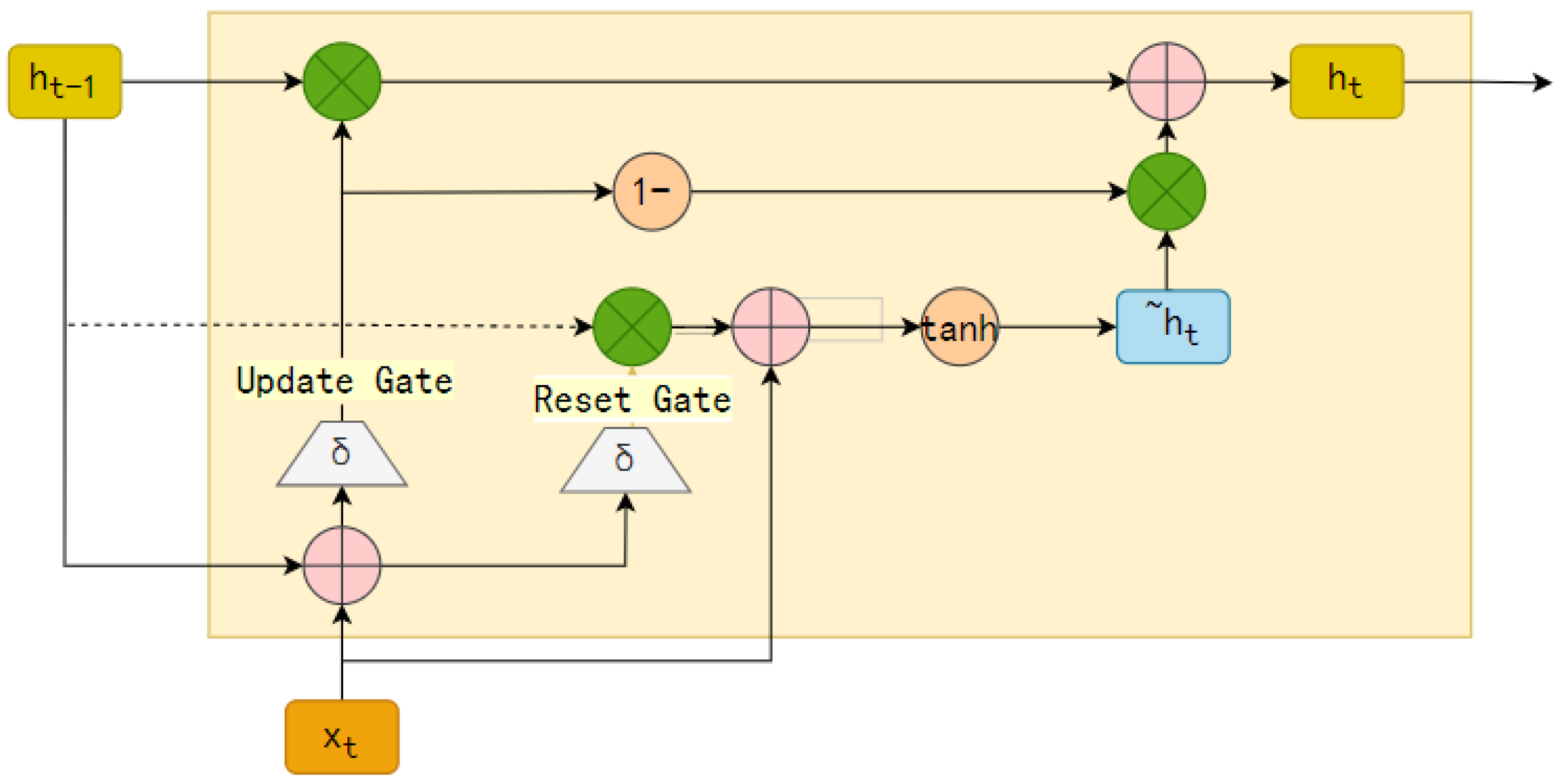A gated recurrent unit optimizes the structure and reduces the number of required parameters while maintaining the memory characteristics of the LSTM, thereby significantly accelerating the training process [23]. In a GRU, there is no distinction made between the internal and external states, and the issues of gradient vanishing and explosion are addressed by introducing a linear dependency between the current network state and the network state from the previous moment. The structure of a GRU network is shown in Figure 1.

In GRU networks, there are two main structures, the update gate and the forget gate. The number of candidate states $\widetilde{h_t}$ to be retained in the output state ${ h}_t$ at the current moment, and the number of historical states $h_{t-1}$ to be retained are controlled by the update gate. The update gate is calculated as follows:

$$z_t=\sigma \left(W_z{x}_t+U_z{h}_{t-1}+b_z\right).$$

(1)

$z_{t }$ is the output of the update gate. This output is then multiplied by the historical state $h_{t-1}$. The candidate state $\widetilde{h_t}$ is multiplied by the factor $1-{\mathrm{z}}_{\mathrm{t}}$. Thus, the final output at the current moment in the network is as follows:

$$h_t=z_t\odot h_{t-1}+(1-z_t)\odot \widetilde{h_t}.$$

(2)

In a GRU network, the candidate state at the current moment $\widetilde{h_t}$ depends on the network state from the previous moment $h_{t-1 }$. This is controlled by the reset gate. The figure illustrates that the network state of the previous moment $h_{t-1}$ is initially multiplied by the output of the reset gate, and then this result is used as a parameter with which to calculate the candidate state of the current moment. The formula for the reset door is as follows:

$$r_t=\sigma (W_r{x}_t+U_r{h}_{t-1}+b_r).$$

(3)

$r_t$ is the output of the reset gate. $r_t$ determines the degree of dependence of the candidate state $\widetilde{h_t}$ on the state of the previous moment $h_{t-1}$. The formula for the candidate state $\widetilde{h_t}$ is as follows:

$$\widetilde{h_t}=tanh(W_c{x}_t+U_c({r_t\odot h}_{t-1})+b_c).$$

(4)

And when the value of $z_t$ is 0 and the value of $r_t$ is 1, the two gates of the GRU network do not function, and the GRU network at this point degenerates into a simple recurrent neural network.

2.2. The Graph Convolutional Network (GCN)

In recent years, deep learning has received widespread attention for its application to tasks related to graph-structured data. The emergence of the graph neural network (GNN) [24,25,26] has led to significant breakthroughs in fields such as social networks, natural language processing, computer vision, and even the life sciences. GNNs can view practical problems as connection and message propagation problems between nodes in a graph, and model the dependencies between the nodes so that they can handle graph-structured data well.

CNNs have achieved significant accomplishments in various fields, such as image recognition and natural language processing [27,28], but they are primarily effective at processing regular Euclidean data, like grids and sequences. They are not adept at handling non-Euclidean data with graph-structure characteristics, such as data within social media networks, chemical composition structure data, biological protein data, and knowledge graph data. For this reason, scholars successfully applied CNNs to graph-structured non-Euclidean data, after their unremitting efforts, by proposing GCNs.

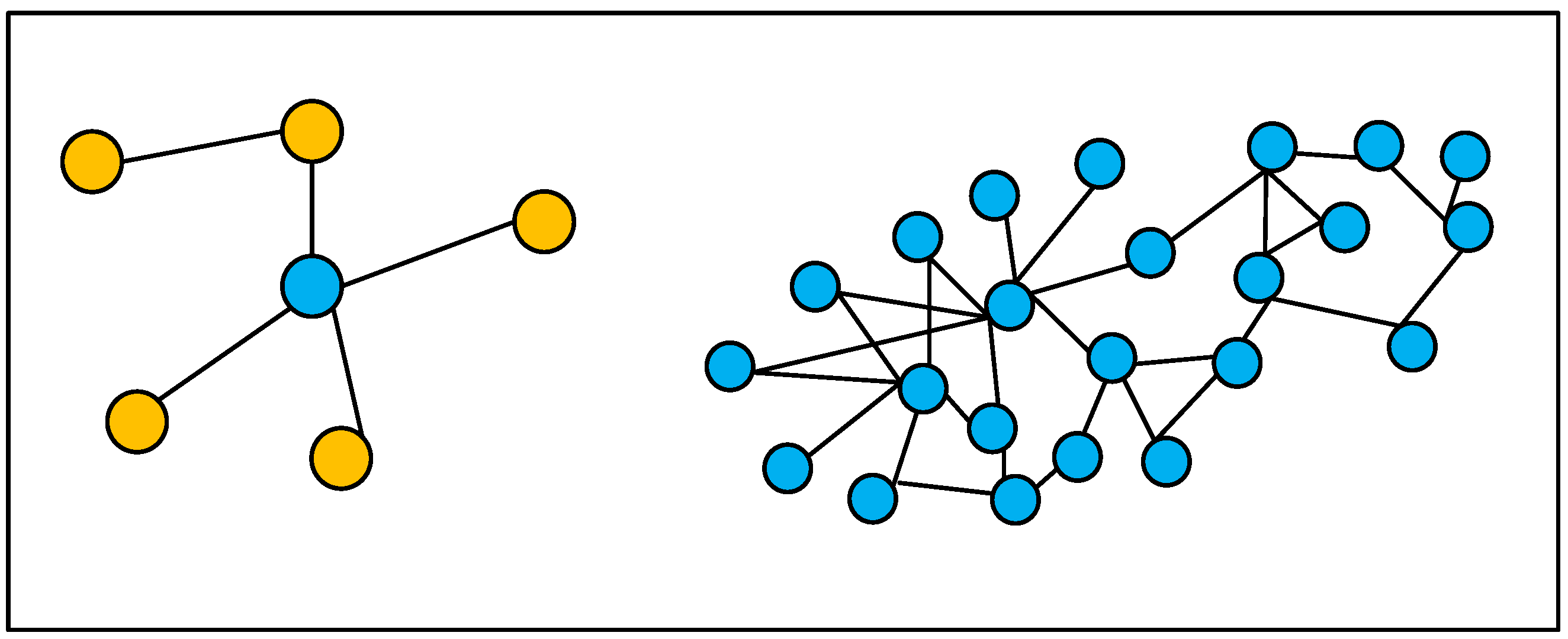
As is well-known, CNNs can access the deep features of data by feature extraction, while a GCN is a natural extension of a CNN’s graph structure. The difference between the two lies in the different objects of research. A CNN uses n × n two-dimensional matrices as a convolution kernel, and Euclidean data with a regular spatial structure are the data type it targets [29,30]. It can be represented by either a one-dimensional or two-dimensional matrix representation. However, for example, brain signals, three-dimensional nodes, communication networks, and the analytical structure of interpersonal networks, such as the abstract formation of graph-structured data, etc.—i.e., data that do not have a specific size and shape—CNNs do not process these well. So it is necessary to use a GCN to deal with these types of data. Of course, a regular structure that can be represented by a two-dimensional matrix belongs to a special form of graph structure, so the data that can be processed by a CNN can theoretically be processed by a GCN, but the data with an irregular topological structure that are commonly processed by a GCN cannot be processed by a CNN. Figure 2 shows two sample graph structures with irregular spatial structures.

A CNN is excellent at extracting the spatial features of graphs, as it uses localized perceptual regions, shared weights, and downsampling over the spatial domain, with stable invariant properties with respect to displacement, scaling, and warping. Graph structures do not have a translation invariant property with respect to pictures, and the number of domain nodes in a graph structure is not exactly the same for each node, as the number of domain nodes is not exactly the same, so the features cannot be extracted with the same size of convolution kernel as in traditional CNNs. Therefore, this type of convolution is not applicable to graph structures.

A GCN is a generalized form of a CNN, and the interactions between each layer of the network share parameters. The way the parameters of the GCN are shared is by using the graph convolution operator in the training process. For this, one needs to randomly designate a node as the starting point, according to the depth-first search and breadth-first search of the graph, etc. Then it iterates over every node in the graph to obtain the features of every node in the graph. During this process, it can not only obtain the self features, but also the features of the domain nodes, and when the network is deeper, the scope of the model learning will be larger, and the information acquired will be deeper. During the initial convolution operation, each node in the graph contains only part of the features of its neighboring nodes, and with an increasing number of convolution layers, the nodes will continuously learn the features of all the surrounding domain nodes. Therefore, in a deep network model, the more features that are encapsulated, the larger the sensory field is, and more advanced features can be obtained.

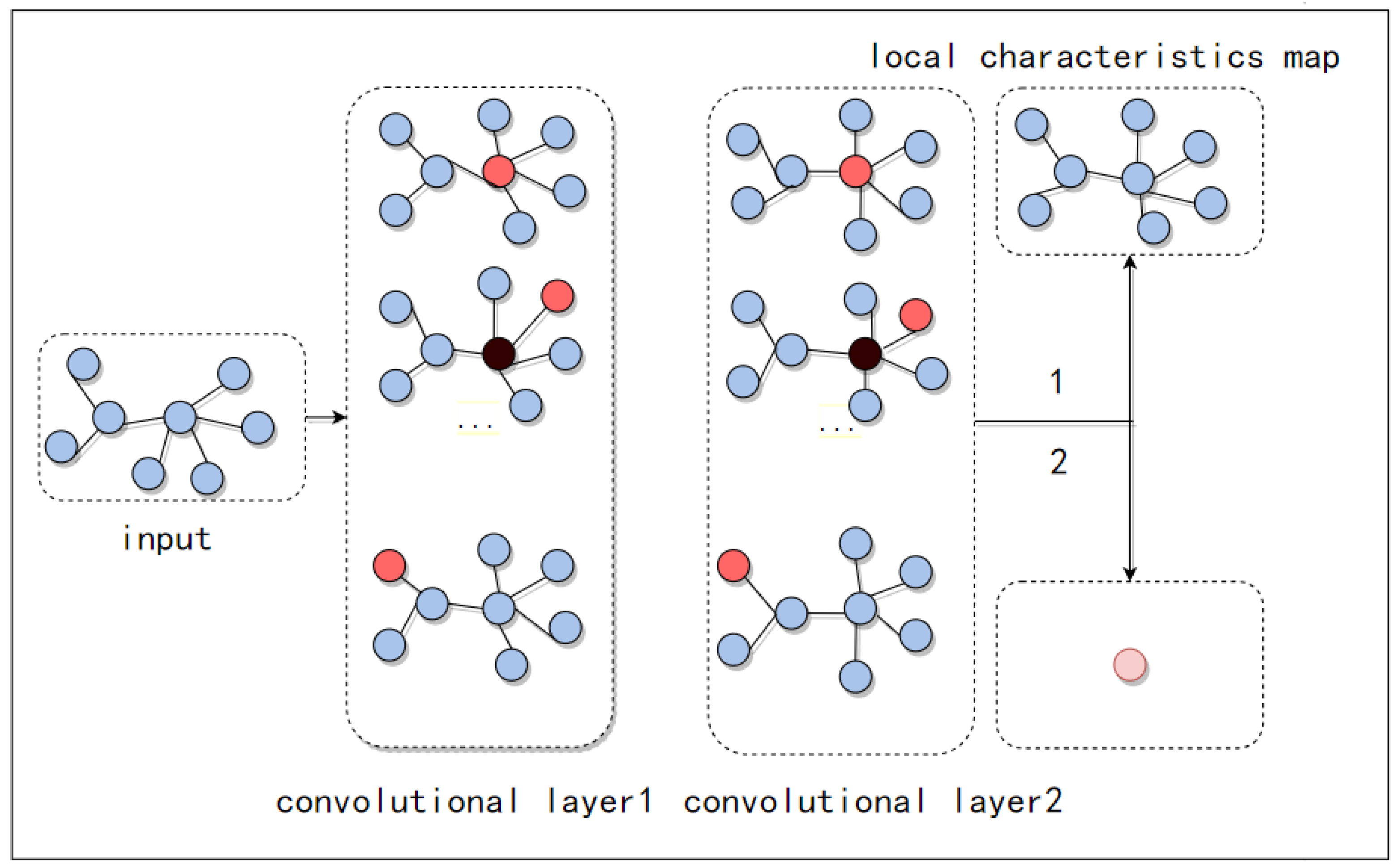
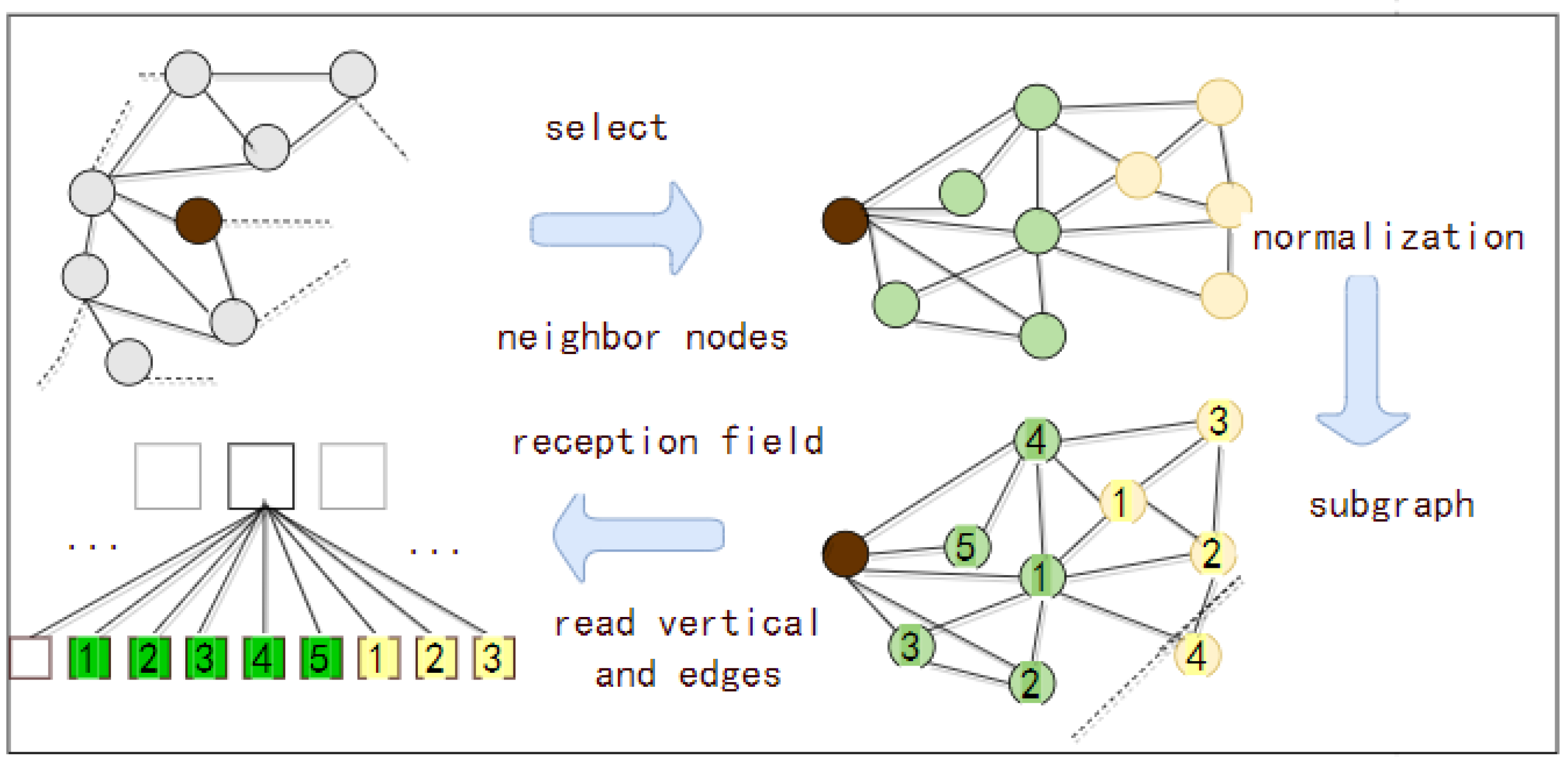
The main framework of a GCN is shown in Figure 3. From the figure, it can be seen that the input layer of the GCN is a graph with an irregular topology, and the graph data will be passed to the convolutional layer after processing. For each convolutional layer, the graph convolution operator performs a convolutional computation on each node in turn; there are a number of layers in each convolutional layer, and after convolution, the global or local features are acquired according to the task. After the process of convolution, the local features can be obtained by mapping the features of each node onto the corresponding position through the local output function. After the process of convolution, the output graph is linearly transformed so that the features of each node in the graph are fused to obtain the global features. In addition, since the input data of the GCN are irregular spatial structure data, the model can be applied to data with any topological structure to improve the generalization ability of the model.

The essence of a GCN is to extract the structural features of the graph; the key is how to define the local receptive field. There are two main ways:

(a)

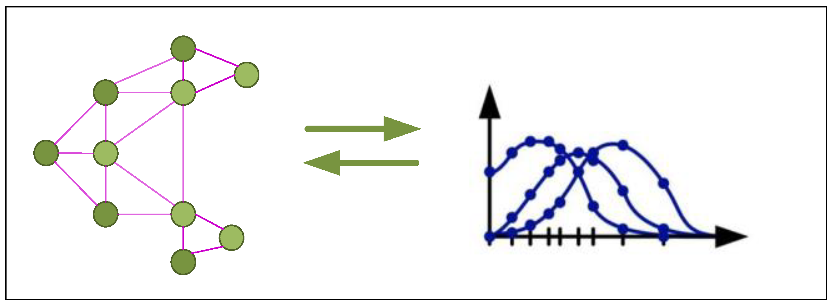
The spectral approach: A spectral domain-based GCN represents the successful adaptation of CNNs to the graph structures by utilizing graph signal processing theory, with the Fourier transform as the link. It operates from a spectral domain perspective and employs Laplacian matrices to manage non-Euclidean structured data like graphs (see Figure 4).

• (b) The spatial approach: A spatial domain-based GCN differs from a spectral domain GCN in its signal processing theory. It is designed from the perspective of the nodes within the graph, defining an aggregation function to integrate the attributes of neighboring nodes, and employing a message-passing mechanism that allows for the surrounding node features to be used effectively and precisely to update the representation of the central node’s characteristics. The procedure is given in Figure 5.

3. Methodology

The overall architecture of the spatiotemporal combination-based transformer error prediction model is shown in Figure 6, which is named the Gated–Temporal Graph Convolution Network (Gated-TGCN). The spatiotemporal combination network prediction model consists of a temporal module, a spatial module, and a spatiotemporal fusion module. The main role of the spatial module is to capture the spatial dependence and the main role of the temporal module is to capture the temporal dependence.

The temporal component is the integration of the multi-head attention mechanism module and the gated recurrent temporal convolutional network module. Between the two modules, an Add and Norm section are introduced, where ‘Add’ represents the residual connection and ‘Norm’ stands for layer normalization. These are employed to mitigate the issue of gradient vanishing in deep models, and to lessen the degradation observed in deep networks. The multi-head self-awareness mechanism is good at capturing the random dependence of time series and correlation within the data or features, so the multi-head self-awareness is used to observe different information in different historical periods. Then, the residuals are connected between two sub-layers, and then a layer normalization is performed. Also, to consider the local and long-term time dependence, the observed information from the multi-head attention mechanism is fed into the gated TCN for time-series modeling. The gated loop unit simplifies the structure and reduces the number of parameters while retaining the memory unit function of the LSTM, thereby significantly improving the training speed.

The spatial module is mainly composed of the adaptive graph convolution network, which contains the graph convolution network module (GCN Module) and the graph attention network module (GAT Module). The Gated Fusion Network is composed of three parts. The inputs for the model are used as inputs for the GCN Module and GAT Module after positional embedding. The essence of a GCN is to extract the structural features of a graph. After convolution, local output functions are used to map the features of each node onto their corresponding positions, thus obtaining the local features. After convolution, a linear transformation on the output graph is performed, so that the features of each node in the graph can be fused to obtain the global features. In this way, more advanced features can be obtained.

Within the whole structure, the gated fusion mechanism is used in two places. Firstly, the gated fusion mechanism is used to fuse the GCN module and GAT module to form the GNN module, which is used to jointly process the non-Euclidean data. Then, the gated fusion mechanism is used to fuse the temporal module and the spatial module, which is used to learn the correlation between space–time and time.

To facilitate the model’s description in this section, a separate problem definition is given for the spatiotemporal combination-based transformer error prediction model. The transformer error prediction model utilizes online monitoring data for the power grid to predict the mutual transformer error. To facilitate the explanation of the spatial distribution characteristics of the sensors in the power grid, the power grid is defined in this section as a graph structure G(V, E, A), where V denotes the set of nodes, i.e., within the target power grid, the sensors form a set; set E represents the edges, which describes the connectivity between the sensors in the road network; and set A is the adjacency matrix, used to indicate the relationship of the connections within the set of edges. There is the following definition:

$$A_{i,j}=\left\{\begin{array}{c}1, <v_i,v_j>\in E\left(G\right)\\ 0, <v_i,v_j>\notin E\left(G\right)\end{array}\right..$$

(5)

where $A_{i,j}$ is the corresponding element of the i-th row and j-th column in the adjacency matrix, and $<v_i,v_j>$ represents the node pair composed of node i and node j.

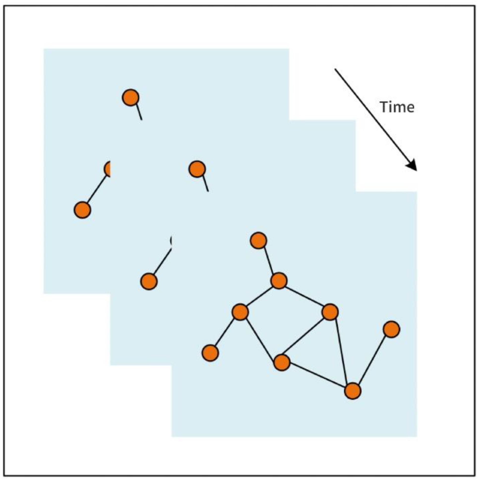
The grid operation state at a particular moment corresponds to a set of graph data; then, the graph data for multiple moments form the spatiotemporal graph data within a continuous observation length, as shown in Figure 7.

For the transformer error prediction task, let us denote the target power grid as a graph structure, denoted as G(V, E, A). Given the spatiotemporal graph data consisting of N sensor nodes with an observation time window length of T, the goal of the prediction task is to use this input data to forecast the intertransformer error values for all the nodes within the grid at H moments in the future.

3.1. The Adaptive Graph Convolutional Network

For the construction of the adaptive graph convolutional networks, two main types of graph neural networks are used–a GCN and GAT. A GCN is a type of spectral-based graph neural network, while a GAT is a type of spatial-based graph neural network. Though both perform well on the problem of handling non-Euclidean data, they have their own advantages in different situations due to different mechanisms. The idea behind the GCN is to use adjacency matrices with weights to generate Laplacian matrices, and then multiply the input matrices by the Laplacian matrices and the parameter matrices that can be learned, respectively. The GAT, on the other hand, uses the adjacency matrix without weights and uses the attention mechanism to automatically generate the weights between the relevant nodes using the trained data. In such a case, the validity of the weight values of the adjacency matrix is very important for the GCN. However, the same adjacency matrix can generate different weights using different computational methods. In addition, since the nodes of the circuit network are generally chosen to set up sensors on roads, they are not exactly de facto road network intersections, and the characteristics of roads with different shapes and curvatures are not the same. All these reasons lead to a difference in the final calculation of the abstract weights from the actual situation. However, on the other hand, there are many reference values for this weight matrix, which can reflect some of the actual characteristics of the circuit network topology to a certain extent. Therefore, it was decided to design a fusion mechanism to fuse the GCN module and the GAT module to jointly capture the spatial dependencies, and the reference used here is the structure of the update gate in the GRU.

In a GRU network, the role of the update gate is to determine how much of the current moment’s output state $h_t$ is preserved by the historical state $h_{t-1}$, and how much is retained by the candidate state $\widetilde{h_t}$. The output of the update gate is multiplied by the historical state $h_{t-1}$ and the candidate state $\widetilde{h_t}$, respectively, where the factor for the candidate state $\widetilde{h_t}$ is $1-z_t$. 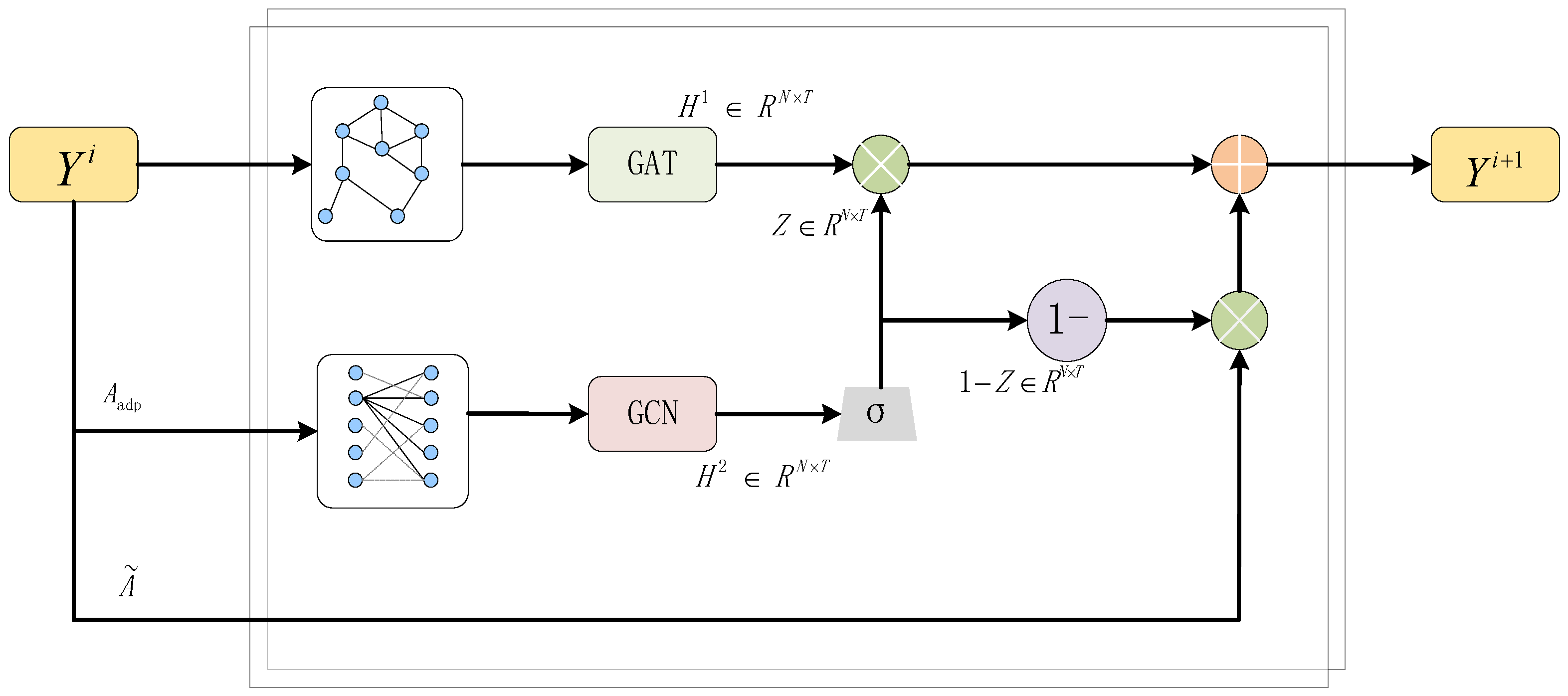Therefore, in the adaptive GCN, the structure of the update gate is borrowed from the GRU, so that each node in each layer of the GNN can be selectively updated and forgotten, as shown in Figure 8. First, the input data matrix Y is entered into the GCN and GAT networks, respectively. The outputs of the GCN network are also passed through the activation function in order to incorporate nonlinearities and improve the overall expressiveness of the model. The variable z is used to control the proportion of weights for gated fusion. The values of each corresponding position of the weight matrix of the two sides of the dot product are summed up to give 1. The gated value z indicates how much information was updated in the next layer, 1 − z indicates how much information was forgotten in the next layer, and the results of the previous layer are used. The result of the graph convolution is then computed using the adaptive adjacency matrix to obtain the gating value z.

The gating value z is obtained from the input matrix of the initial graph neural network module by linear computation, which is followed by the activation function to incorporate nonlinearities and improve the overall expressiveness of the model. Where the input matrix $Y^i\in R^{N\times T}$ is the output matrix of the previous layer of the GNN, when i = 0, $Y^0$ is the input matrix for X. $Y^i\in R^{N\times T}$ is the output matrix of the current layer of the GNN. This enables the selective updating and forgetting of the multilayer GNN, and each node can obtain a more adequate and reasonable high-dimensional feature.

$$Y^{i+1}=z\odot H^1+\left(1-z\right)\odot Y^i,$$

(6)

$$z=\sigma \left(H^2\right).$$

(7)

3.2. The Spatiotemporal Integration Layer

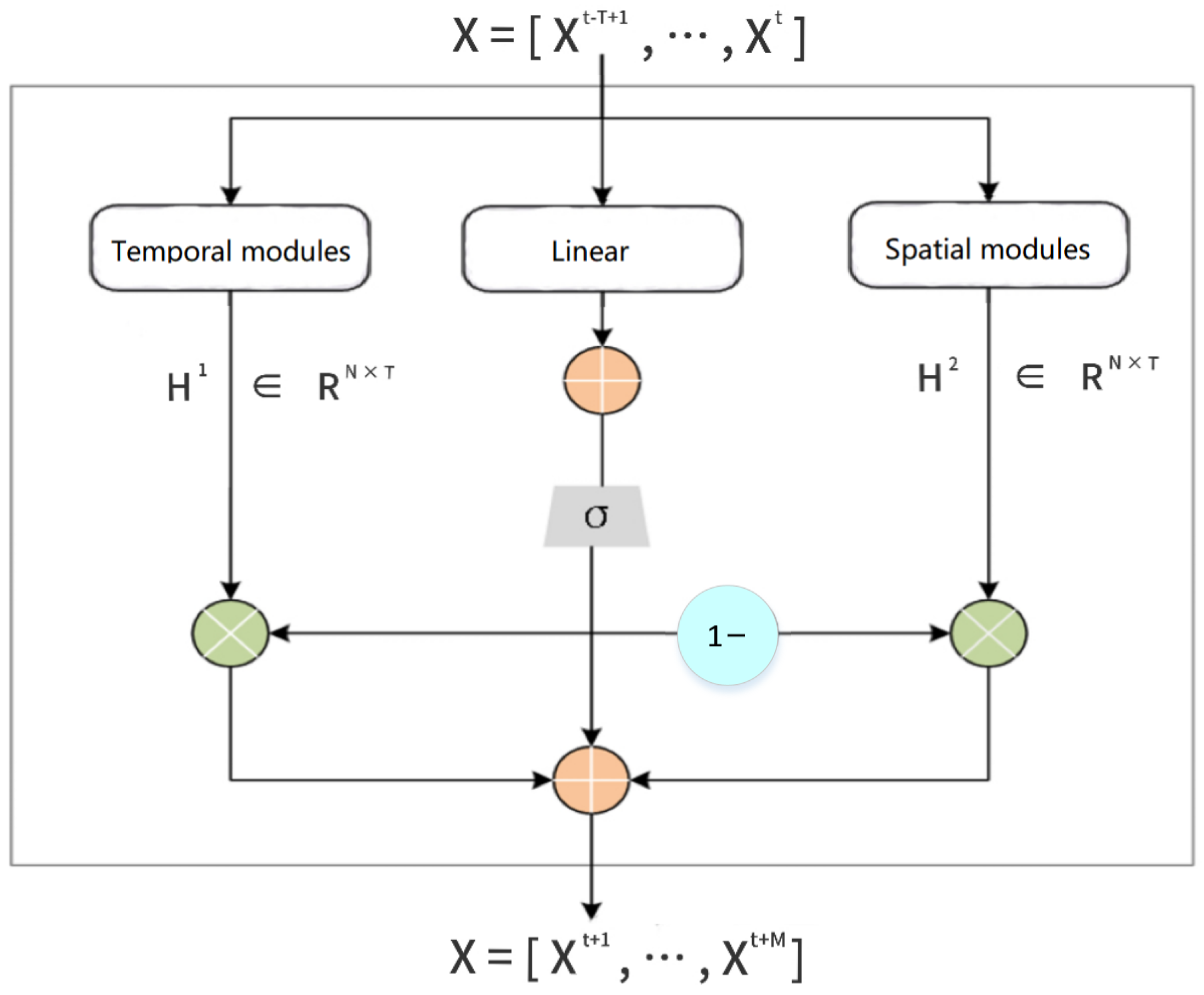
For the transformer operation data, considering the interaction of the temporal and spatial features, the direct passage of the data through the temporal and spatial modules does not always achieve the desired results. Therefore, using the gating fusion mechanism similar to the previous combination of two GNNs to combine the temporal and spatial modules allows the model to learn the temporal and spatial correlations in the data, as shown in Figure 9.

For the fusion of the spatiotemporal modules, the two weight matrices are multiplied by the outputs of the temporal and spatial modules, respectively. The fusion calculation for this step is shown by (8). z is used to control the fusion of the weight ratio. The two sides of the dot product of the weight matrix give a value of 1. The value of z is calculated using the initial input matrix X, the linear calculation, and also through the activation function, as shown by (9):

$$Y=z\odot H^1+\left(1-z\right)\odot H^2,$$

(8)

$$z=\sigma (XW+b)$$

(9)

where $H^1$ and $H^2$ denote the outputs processed by the temporal and spatial modules, respectively.

4. Experiments

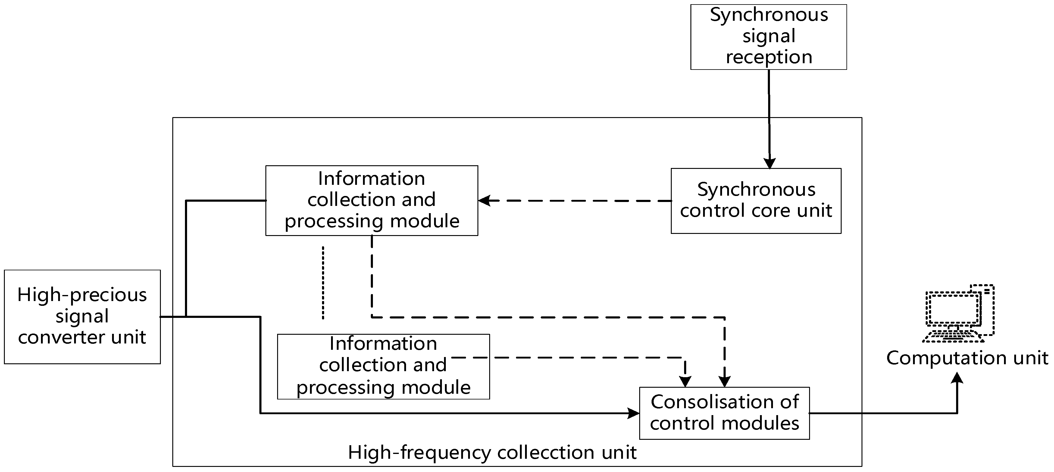
We conducted experiments using 10 days of simulated transformer monitoring data from multiple electric fields; the principle of operation of the device for monitoring the current transformer is shown in Figure 10.

There are 15 test points from which to extract the “amplitude” and the “frequency”—“main transformer group I phase A”, “main transformer group I phase B”, “main transformer group I phase C”, “main transformer group II phase A”, “main transformer group II phase B”, “main transformer group II phase C”, “main transformer group III phase A”, “main transformer group III phase B”, “main transformer group III phase C”, “line 5449 phase A”, “line 5449 phase B”, “line 5449 phase C”, “5450 line A phase “, “5450 line B-phase”, and “5450 line C-phase”— so that there are a total of 16 feature dimensions. Then, combined with the 15 labeling data, there are 356,800 records in total. Next, the processed data were processed to divide them into the training and testing sets according to a ratio of 8:2. The experimental settings were as follows:

(1)

The activation function. This research used the sigmoid function and tanh function as the activation functions.

(2)

The learning rate. The learning rate affects the update of the parameters. If the learning rate is too high, it can lead to explosive and oscillating loss values. If it is too small, it can cause overfitting and slow convergence speeds. Therefore, this research used the trial and error method to determine the best prediction effect. We found that the optimum was achieved when the learning rate was 0.001.

(3)

The batch processing. Based on the traffic data scale of 17,280 × 524 used in this research, we chose batch_size = 32 based on previous experience.

(4)

Model training iterations. Based on manual experience, in this research we set the number of model epochs to 300 to avoid overfitting.

To thoroughly evaluate the performance of our model, we conducted comparative experiments between the proposed Gated-TGCN model and the Spatiotemporal Graph Convolutional Networks (STGCN).

From the experimental results in

Table 1. Experiments comparing Gated-TGCN and STGCN model predictions.

Network Models	MAPE, %	MSE	MAE	RMSE	R2
STGCN	12.35	4800.31	13.38	62.81	0.936
Gated-TGCN	11.46	3909.58	12.54	58.93	0.953

, it can be observed that with respect to the MAPE metric (the mean absolute percentage error), the proposed Gated-TGCN model is better by 7.2% compared to the STGCN network model. Concerning the mean squared error (MSE) metric, the smaller the value is, the higher the accuracy of the prediction model. The observed results indicate that compared to the STGCN network model, the Gated-TGCN network model achieved an absolute reduction of 890.7, which is 18.6%. Concerning the mean absolute error (MAE), the Gated-TGCN model achieved an absolute decrease of 0.84, which is 6.3%.

An absolute reduction of 3.88 was achieved for the root mean square error (RMSE) metric, which is 6.2%. For the coefficient of determination (R²) metric, the closer the value is to 1, the better the predictive performance of the model and fitting are. From the analysis above, it is evident that the Gated-TGCN model achieved an absolute gain of 0.017 in prediction accuracy compared to the STGCN, which is 1.7%. Taking into account the indicators mentioned, it can be concluded that the proposed Gated-TGCN model surpasses the STGCN model for all parameters of predictive capability.

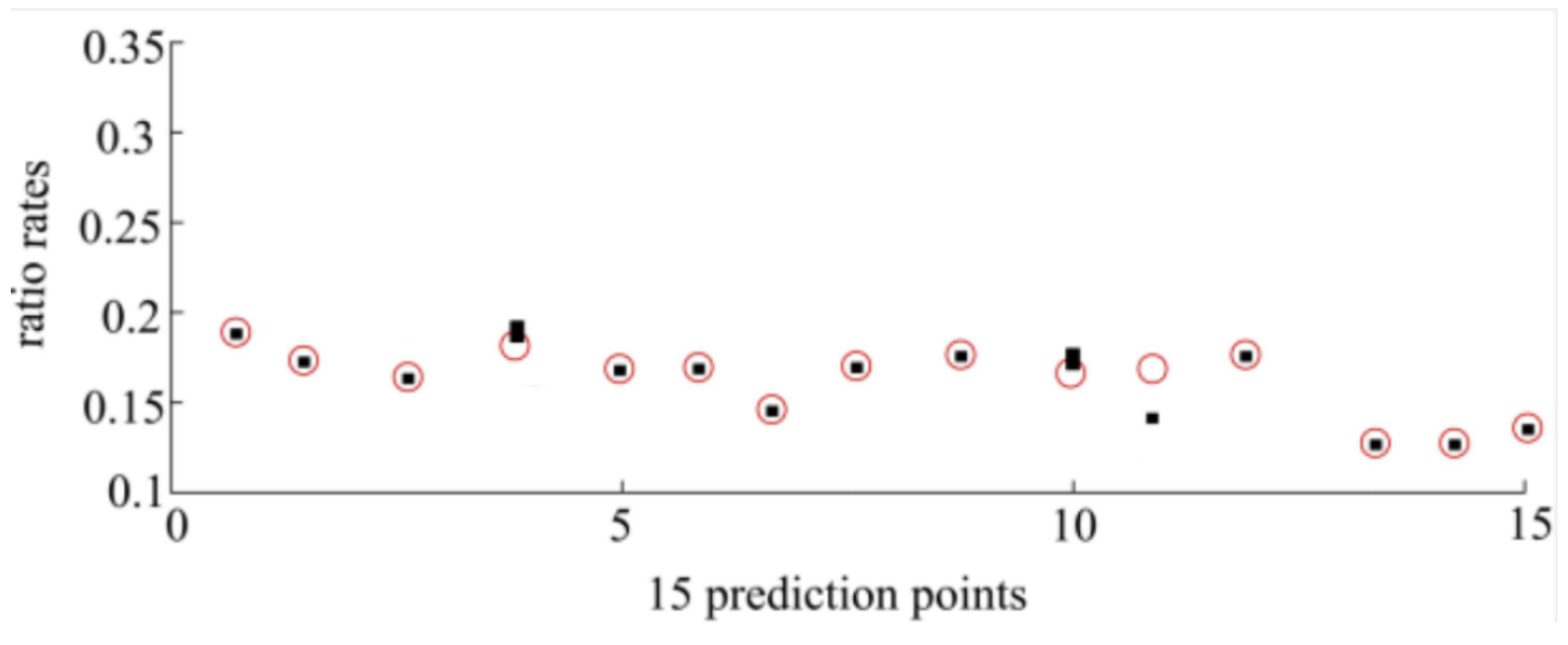
Next, this research used the STGCN model to analyze the fitting errors of the 15 label data using the parallel serial hybrid algorithm. Figure 11 shows the predicted results of the 15 label data.

The red circles in the figure indicate the 15 actual ratio rates, and the black squares indicate the predicted values. It can be seen that most of the predicted values and actual values match at the 15 points, and only some deviations exist in individual points #10 (“Phase A of Line 5449”) and #11 (“Phase B of Line 5449”).

Table 2. Complete errors at each point.

Point Number	Point	Average Absolute Error of Points
1	Main Transformer Group I Phase A	2.783$\times {10}^{-4}$
2	Main Transformer Group I Phase B	2.495$\times {10}^{-5}$
3	Main Transformer Group I Phase C	1.173$\times {10}^{-4}$
4	Main Transformer Group II Phase A	8.253$\times {10}^{-6}$
5	Main Transformer Group II Phase B	5.182$\times {10}^{-6}$
6	Main Transformer Group II Phase C	4.224$\times {10}^{-5}$
7	Main Transformer Group III Phase A	9.788$\times {10}^{-6}$
8	Main Transformer Group III Phase B	7.127$\times {10}^{-5}$
9	Main Transformer Group III Phase C	2.049$\times {10}^{-6}$
10	“Line 5449, phase A”	5.687$\times {10}^{-2}$
11	“Line 5449, phase B”	1.312$\times {10}^{-3}$
12	“Line 5449, phase C”	8.025$\times {10}^{-5}$
13	“Line 5450, phase A”	1.739$\times {10}^{-5}$
14	“Line 5450, phase B”	2.968$\times {10}^{-4}$
15	“Line 5450, phase C”	4.721$\times {10}^{-5}$

presents the complete error for each point. The experimental results indicate that all the prediction errors are minor.

5. Conclusions

Based on the spatiotemporal characteristics of the data, we constructed a time module with an attention mechanism and a gated TCN for time-series processing. We used gating to fuse the GCN and GAT to form an adaptive graph convolutional network, and the spatial module composed of this adaptive GCN for spatial feature processing. The spatiotemporal fusion layer was used to fuse the temporal and spatial modules. A prediction model based on spatiotemporal integration was constructed. We compared the proposed model to the existing one using five metrics as follows: MAPE, MSE, MAE, RMSE, and the coefficient of determination R². For all the metrics, the proposed model achieved considerable gains. The MAPE was improved by 7.2%, the MSE was improved by 18.6%, the MAE was improved by 6.3%, the RMSE was improved by 6.2%, and R² was improved by 1.7%. So we can conclude that the proposed method is better that the existing one.

In the model constructed in this article, the parameters were determined by manual experience and had a high degree of randomness. Therefore, at a later stage, some intelligent optimization algorithms could be combined to optimize these parameters and construct a more excellent spatiotemporal data prediction method.

References

- Velásquez, R.M.A.; Lara, J.V.M. Current transformer failure caused by electric field associated to circuit breaker and pollution in 500 kV substations. Eng. Fail. Anal. 2018, 92, 163–181. [Google Scholar] [CrossRef]
- Dazahra, M.N.; Elmariami, F.; Belfqih, A.; Boukherouaa, J.; Cherkaoui, N.; Lekbich, A. Modernization and Optimization of Traditional Substations for Integration in Smart Grid. In Proceedings of the 2017 International Renewable and Sustainable Energy Conference (IRSEC), Tangier, Morocco, 4–7 December 2017; pp. 1–4. [Google Scholar]
- Topolskiy, D.V.; Yumagulov, N.I.; Galiyev, A.L. Development of Technical Solutions for Digital Substations Using Ddigital Instrument Combined Current and Voltage Transformers. In Proceedings of the 2018 International Conference on Industrial Engineering, Applications and Manufacturing (ICIEAM), Moscow, Russia, 15–18 May 2018; pp. 1–5. [Google Scholar]
- Topolsky, D.V.; Topolskaya, I.G.; Topolsky, N.D. Intelligent instrument transformer for control systems of digital substations. In Proceedings of the 2018 Ural Symposium on Biomedical Engineering, Radioelectronics and Information Technology (USBEREIT), Yekaterinburg, Russia, 7–8 May 2018; pp. 174–178. [Google Scholar]
- Zhang, Z.; Li, H.; Tang, D.; Hu, C.; Jiao, Y. Monitoring the metering performance of an electronic voltage transformer on-line based on cyber-physics correlation analysis. Meas. Sci. Technol. 2017, 28, 105015. [Google Scholar] [CrossRef]
- Lei, T.; Faifer, M.; Ottoboni, R.; Toscani, S. On-line fault detection technique for voltage transformers. Measurement 2017, 108, 193–200. [Google Scholar] [CrossRef]
- Medeiros, R.P.; Costa, F.B. A wavelet-based transformer differential protection with differential current transformer saturation and cross-country fault detection. IEEE Trans. Power Deliv. 2017, 33, 789–799. [Google Scholar] [CrossRef]
- Ronanki, D.; Williamson, S.S. Evolution of power converter topologies and technical considerations of power electronic transformer-based rolling stock architectures. IEEE Trans. Transp. Electrif. 2017, 4, 211–219. [Google Scholar] [CrossRef]
- Van Der Westhuizen, J.; Lasenby, J. The unreasonable effectiveness of the forget gate. arXiv 2018, arXiv:1804.04849. [Google Scholar]
- Sutskever, I.; Vinyals, O.; Le, Q.V. Sequence to sequence learning with neural networks. Adv. Neural Inf. Process. Syst. 2014, 27, 3104–3112. [Google Scholar]
- Cho, K.; Van Merriënboer, B.; Bahdanau, D.; Bengio, Y. On the properties of neural machine translation: Encoder-decoder approaches. arXiv 2014, arXiv:1409.1259. [Google Scholar]
- Xu, J.; Zuo, W.; Liang, S.; Wang, Y. Causal relation extraction based on graph attention networks. J. Comput. Res. Dev. 2020, 57, 159–174. [Google Scholar]
- Sun, L.; Qin, H.; Przystupa, K.; Cui, Y.; Kochan, O.; Skowron, M.; Su, J. A Hybrid Feature Selection Framework Using Improved Sine Cosine Algorithm with Metaheuristic Techniques. Energies 2022, 15, 3485. [Google Scholar] [CrossRef]
- Su, J.; Beshley, M.; Przystupa, K.; Kochan, O.; Rusyn, B.; Stanisławski, R.; Yaremko, O.; Majka, M.; Beshley, H.; Demydov, I.; et al. 5G multi-tier radio access network planning based on Voronoi diagram. Measurement 2022, 192, 110814. [Google Scholar] [CrossRef]
- Ali, M.N.; Amer, M.; Elsisi, M. Reliable IoT paradigm with ensemble machine learning for faults diagnosis of power transformers considering adversarial attacks. IEEE Trans. Instrum. Meas. 2023, 72, 3525413. [Google Scholar] [CrossRef]
- Tran, M.Q.; Amer, M.; Abdelaziz, A.Y.; Dai, H.J.; Liu, M.K.; Elsisi, M. Robust fault recognition and correction scheme for induction motors using an effective IoT with deep learning approach. Measurement 2023, 207, 112398. [Google Scholar] [CrossRef]
- Przystupa, K. Selected Methods for Improving Power Reliability. Prz. Elektrotech. 2018, 94, 270–273. [Google Scholar] [CrossRef]
- Sun, L.; Qin, H.; Przystupa, K.; Majka, M.; Kochan, O. Individualized Short-Term Electric Load Forecasting Using Data-Driven Meta-Heuristic Method Based on LSTM Network. Sensors 2022, 22, 7900. [Google Scholar] [CrossRef]
- Niu, Z.; Zhong, G.; Yue, G.; Wang, L.N.; Yu, H.; Ling, X.; Dong, J. Recurrent attention unit: A new gated recurrent unit for long-term memory of important parts in sequential data. Neurocomputing 2023, 517, 1–9. [Google Scholar] [CrossRef]
- Xu, X.; Hu, S.; Shao, H.; Shi, P.; Li, R.; Li, D. A spatio-temporal forecasting model using optimally weighted graph convolutional network and gated recurrent unit for wind speed of different sites distributed in an offshore wind farm. Energy 2023, 284, 128565. [Google Scholar] [CrossRef]
- Pradhan, A.; Yajnik, A. Parts-of-speech tagging of Nepali texts with Bidirectional LSTM, Conditional Random Fields and HMM. Multimed. Tools Appl. 2023, 83, 9893–9909. [Google Scholar] [CrossRef]
- Wang, K.; Hua, Y.; Huang, L.; Guo, X.; Liu, X.; Ma, Z.; Ma, R.; Jiang, X. A novel GA-LSTM-based prediction method of ship energy usage based on the characteristics analysis of operational data. Energy 2023, 282, 128910. [Google Scholar] [CrossRef]
- Bilgili, M.; Pinar, E. Gross electricity consumption forecasting using LSTM and SARIMA approaches: A case study of Türkiye. Energy 2023, 284, 128575. [Google Scholar] [CrossRef]
- Gao, M.; Yu, J.; Yang, Z.; Zhao, J. A Physics-Guided Graph Convolution Neural Network for Optimal Power Flow. IEEE Trans. Power Syst. 2023, 39, 380–390. [Google Scholar] [CrossRef]
- Vincent, E.; Korki, M.; Seyedmahmoudian, M.; Stojcevski, A.; Mekhilef, S. Detection of false data injection attacks in cyber–physical systems using graph convolutional network. Electr. Power Syst. Res. 2023, 217, 109118. [Google Scholar] [CrossRef]
- Yan, Y.; Han, Y.; Qi, D.; Lin, J.; Yang, Z.; Jin, L. Multi-label image recognition for electric power equipment inspection based on multi-scale dynamic graph convolution network. Energy Rep. 2023, 9, 1928–1937. [Google Scholar] [CrossRef]
- Yan, L.; Fu, J.; Wang, C.; Ye, Z.; Chen, H.; Ling, H. Enhanced network optimized generative adversarial network for image enhancement. Multimed. Tools Appl. 2021, 80, 14363–14381. [Google Scholar] [CrossRef]
- Yan, L.; Lu, H.; Wang, C.; Ye, Z.; Chen, H.; Ling, H. Deep linear discriminant analysis hashing for image retrieval. Multimed. Tools Appl. 2019, 78, 15101–15119. [Google Scholar] [CrossRef]
- Yan, L.; Zheng, K.; Xia, J.; Li, K.; Ling, H. LMix: Regularization strategy for convolutional neural networks. Signal Image Video Process. 2023, 17, 1245–1253. [Google Scholar] [CrossRef]
- Yan, L.; Sheng, M.; Wang, C.; Gao, R.; Yu, H. Hybrid neural networks based facial expression recognition for smart city. Multimed. Tools Appl. 2022, 81, 319–342. [Google Scholar] [CrossRef]