Artificial Intelligence for Energy Theft Detection in Distribution Networks

Abstract

The digitization of distribution power systems has revolutionized the way data are collected and analyzed. In this paper, the critical task of harnessing this information to identify irregularities and anomalies in electricity consumption is tackled. The focus is on detecting non-technical losses (NTLs) and energy theft within distribution networks. A comprehensive overview of the methodologies employed to uncover NTLs and energy theft is presented, leveraging measurements of electricity consumption. The most common scenarios and prevalent cases of anomalies and theft among consumers are identified. Additionally, statistical indicators tailored to specific anomalies are proposed. In this research paper, the practical implementation of numerous artificial intelligence (AI) algorithms, including the artificial neural network (ANN), ANFIS, autoencoder neural network, and K-mean clustering, is highlighted. These algorithms play a central role in our research, and our primary objective is to showcase their effectiveness in identifying NTLs. Real-world data sourced directly from distribution networks are utilized. Additionally, we carefully assess how well statistical methods work and compare them to AI techniques by testing them with real data. The artificial neural network (ANN) accurately identifies various consumer types, exhibiting a frequency error of 7.62%. In contrast, the K-means algorithm shows a slightly higher frequency error of 9.26%, while the adaptive neuro-fuzzy inference system (ANFIS) fails to detect the initial anomaly type, resulting in a frequency error of 11.11%. Our research suggests that AI can make finding irregularities in electricity consumption even more effective. This approach, especially when using data from smart meters, can help us discover problems and safeguard distribution networks.

1. Introduction

Detecting energy theft and NTLs in distribution power networks is essential for financial stability, equitable cost sharing, sustainability, reliability, compliance, and data-driven optimization. It represents a pivotal step towards building a robust, efficient, and fair energy distribution system. By detecting and addressing these losses, the reliability and quality of electricity supply can be improved, enhancing customer satisfaction. Minimizing NTLs contributes to the conservation of resources and aligns with environmental conservation goals. Detecting NTLs is crucial for two key reasons. Firstly, it helps cut down on financial losses. Secondly, it enhances the reliability and security of distribution networks. The digitization of low-voltage networks and the deployment of smart meters have opened up opportunities for the implementation of various techniques for this purpose. The size of electrical distribution network datasets has been growing exponentially due to the widespread adoption of smart metering projects worldwide [1]. Big data, AI, and various optimization methods have become the main tools for the decision making process, operation, and control of smart grids. Therefore, AI for NTL detection has the potential to become part of the standard toolbox for distribution grid controllers.

Reviews [2,3,4,5,6] have explored the diverse range of measurements applicable to distribution system operators (DSOs) and smart grids for the detection of non-technical and commercial losses, as well as the theft of electricity. Reference [7] introduces an intelligent energy meter that provides a comprehensive solution for maintaining power quality, billing, and controlling power theft. Another paper [8] focuses on preventing power theft in distribution systems using smart hardware devices. A further paper [9] utilizes state-of-the-art gradient boosting classifiers to detect energy theft in distribution power systems. In contrast, [10] presents a data analytic approach involving the injection of false data. Furthermore, [11] proposes an IoT solution for electricity theft prevention. For electricity theft detection, two methodologies are discussed in [12,13]: the stacked sparse denoising autoencoder; and the support vector machine. The authors of [14] employ a variety of data sources to identify manipulated electricity meters using a metric inspired by entropy. Another paper [15] introduces a pattern-based and context-aware approach for detecting electricity theft. A further paper [16] uses an ANN for specific energy theft detection in IEEE 13-node distribution systems with a small number of consumers. The ANFIS methodology is originally presented in [17] using the inputs of mean, median, load factor, and other indicators calculated from consumer electricity consumption. The authors did not use characteristic load diagram indicators, but only mathematical indicators. In another paper [18], autoencoder neural networks are showcased for extracting abstract behavioral traits from electricity data, thereby establishing an initial alert system for identifying electricity theft behavior. Moreover, K-means clustering is utilized to assess users within abnormal distribution regions. Furthermore, the authors of [19] explore the potential correlation between alterations in electricity consumption by individual users and the corresponding shift in line loss rates within their station area through a correlation analysis. The authors of [20] described 120 features of a set of energy consumption data, which included statistics, ratios, and distributions. In these papers, the authors have not compared different machine learning (ML) techniques with statistical parameters or serial sets of numerical consumption inputs. The ML algorithms should not be tied to a specific test network but should provide a general concept and be applicable to the consumption data of any distribution network.

ML enables computers to learn and improve their performance without being explicitly programmed to do that. In the distribution power system, there exists a vast number of consumers and measurements that require processing and analyses to derive meaningful conclusions. Machine learning is well suited for this task as it leverages a combination of statistics, optimization, linear algebra, graph theory, and functional analyses to enable such capabilities. That is why this paper examines the possibility of applying ML algorithms. ML techniques can be divided into supervised and unsupervised learning. Inputs for ML algorithms can include time series data of consumption or other indicators derived from these measurements. In supervised machine learning, it is essential to have corresponding output data for each set of input data. This implies that within the measurement database, it must be documented whether a particular consumer is honest or not. Unsupervised machine learning, unlike supervised methods, does not rely on specific output data. Instead, it can group consumers based on similar energy consumption patterns and also highlight the presence of energy theft and anomalies when they occur. This paper presents five methodologies for anomaly detection, one of which is based on key statistical indicators. The classical methodology does not provide such successful results, and it has been replaced by the following: the ANN, ANFIS, autoencoder neural network, and K-mean clustering. These four ML algorithms were chosen because they offer clear functionality and intuitively indicate how inputs, statistical parameters or just energy consumption samples, can be used for anomaly detection and energy theft purposes.

The main contributions of this paper are as follows:

• The ANN, ANFIS, autoencoder neural network, and K-mean clustering are applied for power theft detection in a low-voltage power distribution network with 91 consumers using 15 min annual measurements;
• Five different realistic scenarios of possible anomalies are established and presented analytically with statistical indicators;
• The results of four proposed ML algorithms are compared, using energy meter measurements, as well as statistical indicators as inputs;
• The ML algorithms have high success rates for power theft detection, and the classification of the anomaly type was achieved;
• Our well-presented application algorithm can be easily replicated in other databases and distribution power systems.

The initial section of this paper introduces the statistical methodology used for NTL detection. The subsequent sections delve into the application of supervised machine learning techniques, such as the ANN, ANFIS, and autoencoders. The sixth section demonstrates the implementation of the K-mean algorithm as part of unsupervised ML. In the final section, we present the results, comparing all the mentioned methodologies and shedding light on their respective advantages and disadvantages when applied to NTL detection.

2. Statistical Indicators and Methodology

Statistical indicators and simple if/then rules can be used to detect NTLs [21]. The approach presented depends on load diagrams which appear in different formats, such as daily, weekly, monthly, and yearly diagrams. These diagrams are primarily shaped by the daily load diagram, which is influenced by factors such as the characteristics of the consumer area, the arrangement of individual consumers within distinct consumer groups, seasonal fluctuations (e.g., summer or winter), and other relevant considerations [1]. The daily load diagram comprises three core indicators: the maximum daily load (P_max [kW]), minimum daily load (P_min [kW]), and total daily consumed energy (W [kWh]). Other characteristic indicators are defined from the basic indicators as follows:

$$P_{mean}=\frac{W}{24}$$

(1)

$$m=\frac{W}{24P_{max}}$$

(2)

$$T=\frac{W}{P_{max}}$$

(3)

$$n=\frac{P_{min}}{P_{max}}$$

(4)

where P_mean—the daily mean load, m—the daily load factor, T—the time of maximum power utilization, and n—the ratio of the daily minimum to the maximum. The statistical indicators for anomaly detection are derived from preceding metrics, with their corresponding formulas detailed in

Table 1. Statistical indicators for anomaly detection.

Indicator	Description Code
Coefficient of variation	$a_1=\frac{P_{max}}{P_{min}}$
Ratio between peak and valley load	$a_2=\frac{P_{min}}{P_{max}}$
Ratio between peak and average load	$a_3=\frac{P_{max}}{P_{mean}}$
Valley coefficient	$a_4={\mathrm{m}\mathrm{a}\mathrm{x}(P}_{i+1}-P_i)$
Load variance	$a_5={\mathrm{s}\mathrm{u}\mathrm{m}(\mathsf{\Delta }P}_i)$
Time of maximum power utilization	$\mathrm{T}=\frac{sum\left(\mathrm{P}\right)}{P_{max}}$

. These statistical indicators are presented and explained in [20,21]. The coefficient of variation is a statistical measure that represents the ratio of the standard deviation to the mean of a dataset. It measures the relative variability of a dataset, allowing for a comparison of the variability between datasets with different units or scales. The ratio between the peak and valley load is a measure that quantifies the difference between the maximum, peak, and minimum loads within a given period. The ratio between the peak and average load measures the relationship between the maximum load and the mean load over a specific period. The valley coefficient is a metric used to quantify the depth or magnitude of the lowest load points within a load profile. The load variance measures the dispersion or spread of load values around the mean load within a dataset. The time of maximum power utilization refers to the point in time when the electricity consumption reaches its peak within a given period.

The most straightforward approach to detect NTLs (non-technical losses) entails comparing characteristic indicators extracted from load diagrams for typical anomalies. By analyzing load diagrams from both customers with and without incidences of electricity theft, it becomes possible to determine the threshold values for these indicators.

In instances in which data from customers involved in theft are lacking, it becomes necessary to develop separate diagrams highlighting specific anomalies. The prevalent types of electrical energy theft observed in distribution system operators (DSOs) can be categorized as follows [21]:

• Multiplying all samples by the same randomly chosen value (lower than one);
• “On/off” attack in which the consumption is reported as zero during some intervals;
• Multiplying the consumption by a random value that varies over time;
• The combination of the second and the third type;
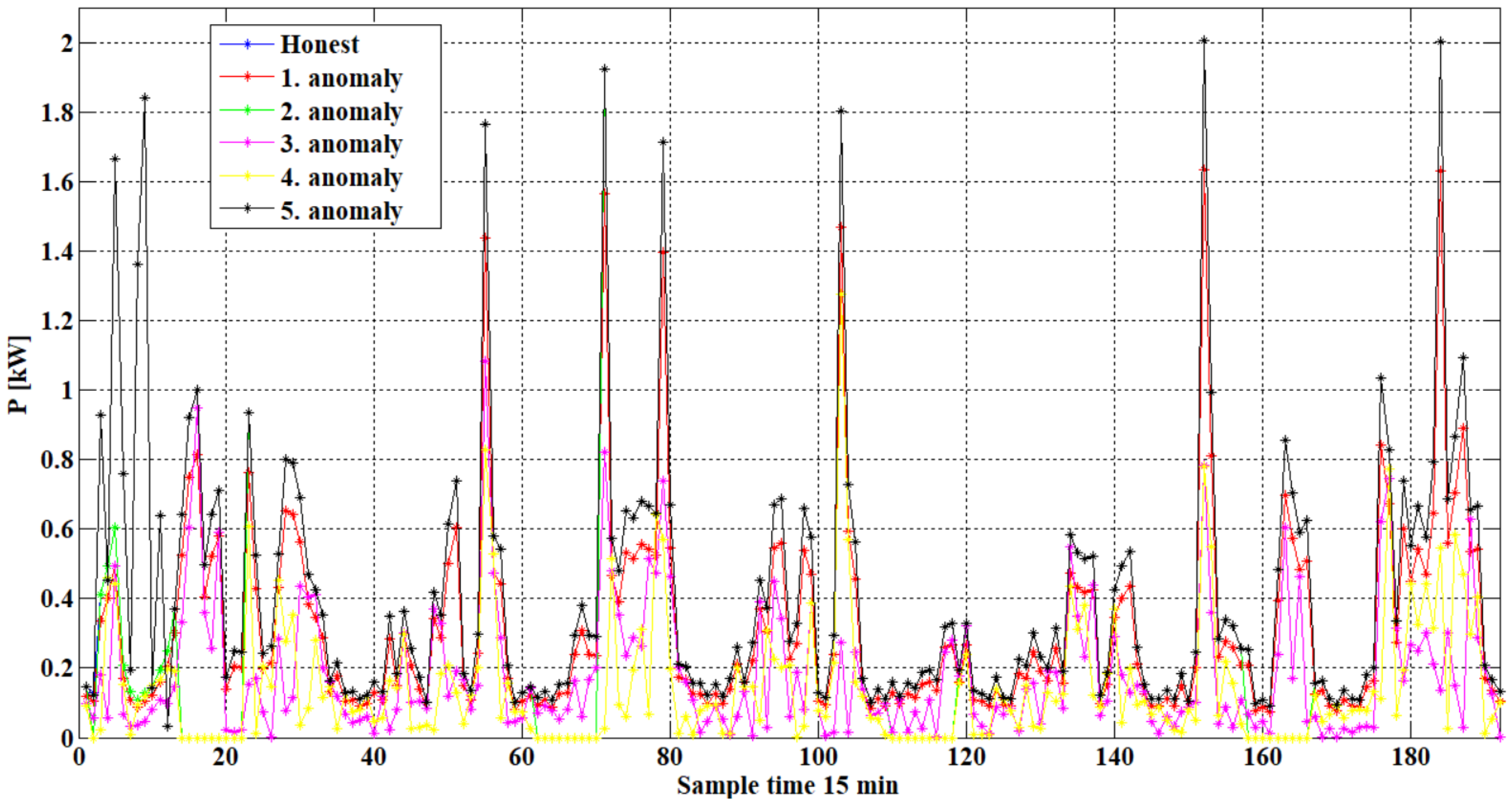
• Multiplying only the peak loads by the same randomly selected value (lower than one).

A computer simulation is utilized to generate all five anomalies using a dataset of real 15 min consumption measurements collected over the course of one week from a household. The obtained annual diagrams for a two-day period are presented in Figure 1. The same process is conducted for 91 households from the same DSO distribution area. For all the created diagrams, the statistical indicators are calculated, and their mean values are presented in

Table 2. Mean vales for statistical indicators for anomaly detection.

Indicators	Honest	1. anom.	2. anom.	3. anom.	4. anom.	5. anom.
a1	43.21	4.37 × 1015	8.12 × 1015	4.31 × 1015	6.06 × 1015	4.61 × 1015
a2	0.0365	0.0356	0	0	0	0.0353
a3	9.17	9.27	11.13	13.37	15.40	9.47
a4	1.46	1.21	1.43	1.20	1.15	1.46
a5	85.78	70.36	75.11	67.56	60.66	85.67
T	105.23	103.67	87.95	70.20	60.44	104.48

. The second column numbers indicate the limit values for the statistical indicators. These values can be used for if/then rules to detect anomalies in that distribution area.

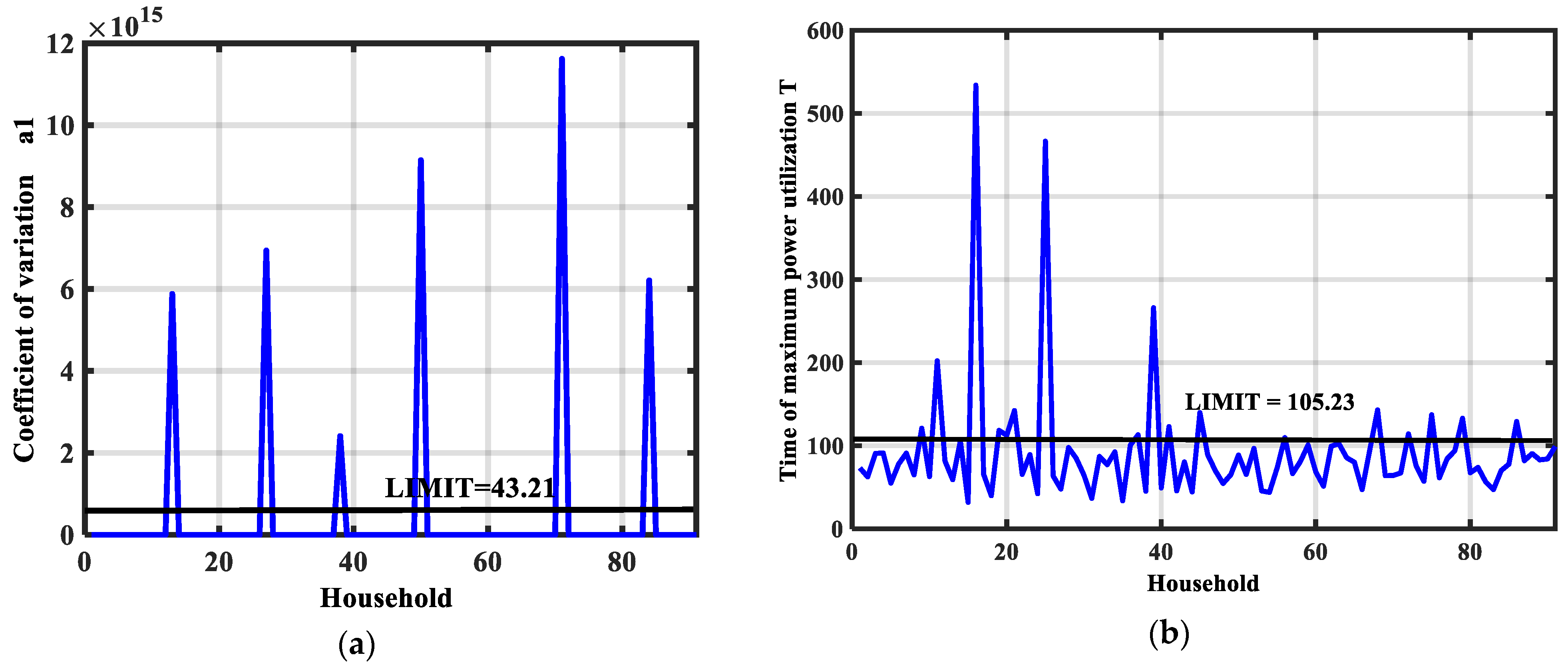
Based on the created data, it can be concluded that the conditions that indicate anomalies in the observed distribution network are as follows: a₁ > 43.21, a₂ < 0.0365, a₃ > 9.17, a₄ < 1.46, a₅ < 85.78, and T < 105.2327. The following diagrams show the values of indicator a₁ and T for all 91 observed households.

As observed in Figure 2a, some consumers clearly exhibit signs of anomalies and electricity theft. However, in Figure 2b, the indications are less distinct, with a significant number of consumers categorized as having NTLs. This becomes particularly concerning when dealing with a larger consumer base. In such cases, the need arises for machine learning methods capable of comparing all consumers and their respective indicators to automatically flag instances of NTLs. The coefficient of variation does not capture specific patterns within the load profile and may not differentiate between different types of anomalies. The ratios between the peak and some other load might oversimplify complex load variations, be sensitive to outliers, or overlook gradual changes or subtle anomalies in the load profile. The valley coefficient might miss gradual deviations from normal patterns. The load variance might not capture temporal correlations or specific load patterns. Indicator T does not consider other aspects of the load profile and may not capture changes in usage intensity. The example shows that there is no clear definition of individual parameters, and it is necessary to combine all of them in order to detect NTLs. In this sense, AI techniques enable the observation of all statistical indicators and the learning of the patterns that exist among them.

3. Artificial Neural Networks

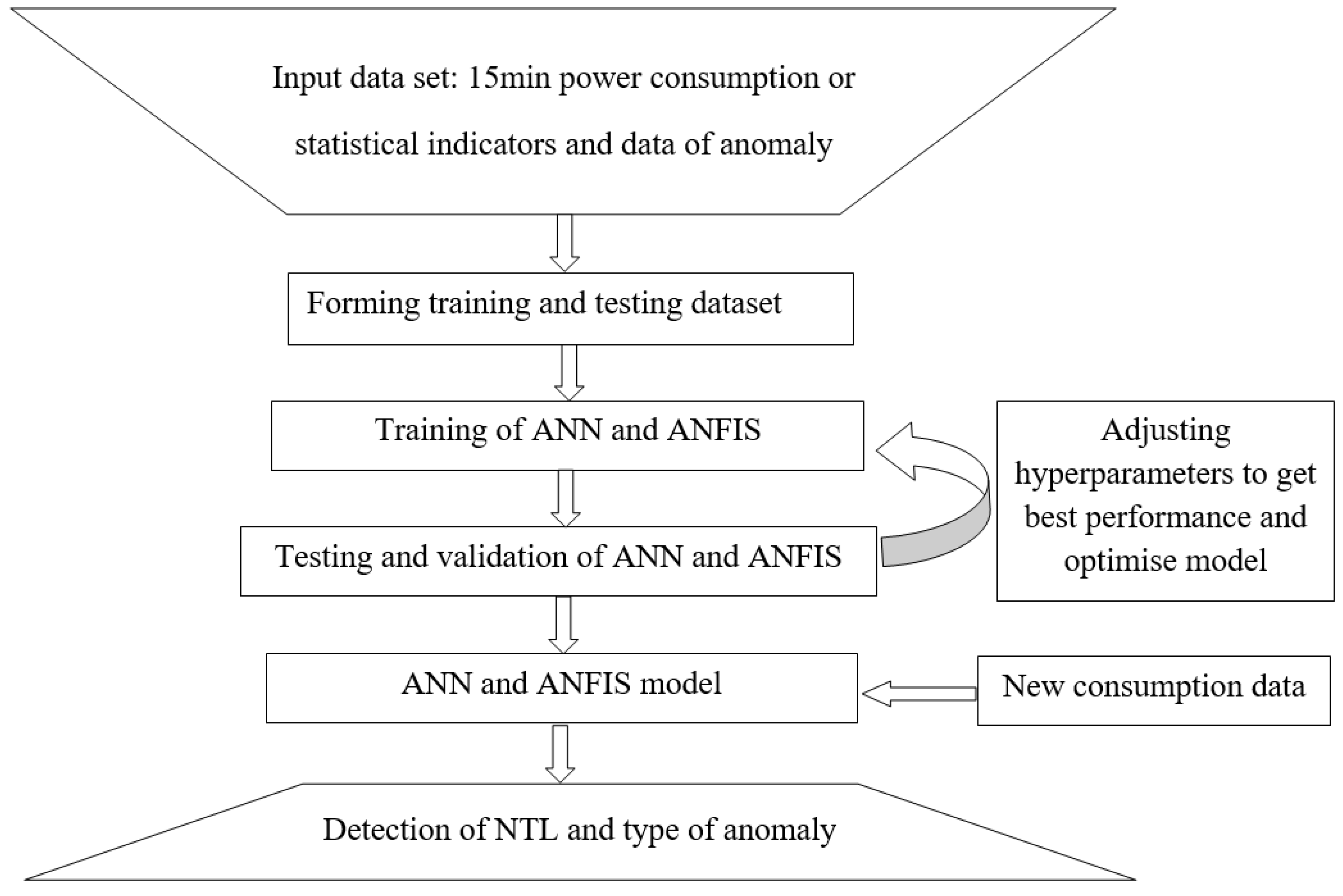
Artificial neural networks, ANNs, as a part of supervised ML, are information processing systems that show the features of learning and generalization based on the data they are trained on. These networks consist of many densely connected processor elements, so-called neurons, which are organized according to some regular architectures. The ANN is used for the problem of supervised learning, in which there is a database with inputs x and exact output values y. The database is structured to include a time series of 91 consumption records without anomalies every 15 min for one year, denoted by an output value of 0. Additionally, it contains simulations of five distinct anomalies, each assigned a unique output value ranging from 1 to 5. The inputs (x) are time series of consumption with and without anomalies. The outputs (y) are indicators from 0 to 5. The concept is to train an artificial neural network (ANN) capable of detecting anomalies, specifically NTLs, and providing insights into the likely type of anomaly involved. At the beginning, the database is randomly divided into 20, 60, and 20% for testing, training, and validation, respectively. The test data are not used until the end of the ANN’s design. The validation data are used to learn the best hyperparameters of the optimized ANN model. The hyperparameter learning process, known as cross-validation, involves training the ANN with various combinations of hyperparameters on the training data, while assessing its performance on the validation data. The training the ANN is accomplished through the backpropagation algorithm. The frequency of error serves as a performance metric to evaluate the model’s prediction accuracy. The ideal ANN configuration consists of three layers with the following number of neurons: 60, 30, and 10. More layers lead to overfitting and increase the error.

The sigmoid function is used, as it is the most frequently used activation function. The ANN application algorithm is shown in Figure 3.

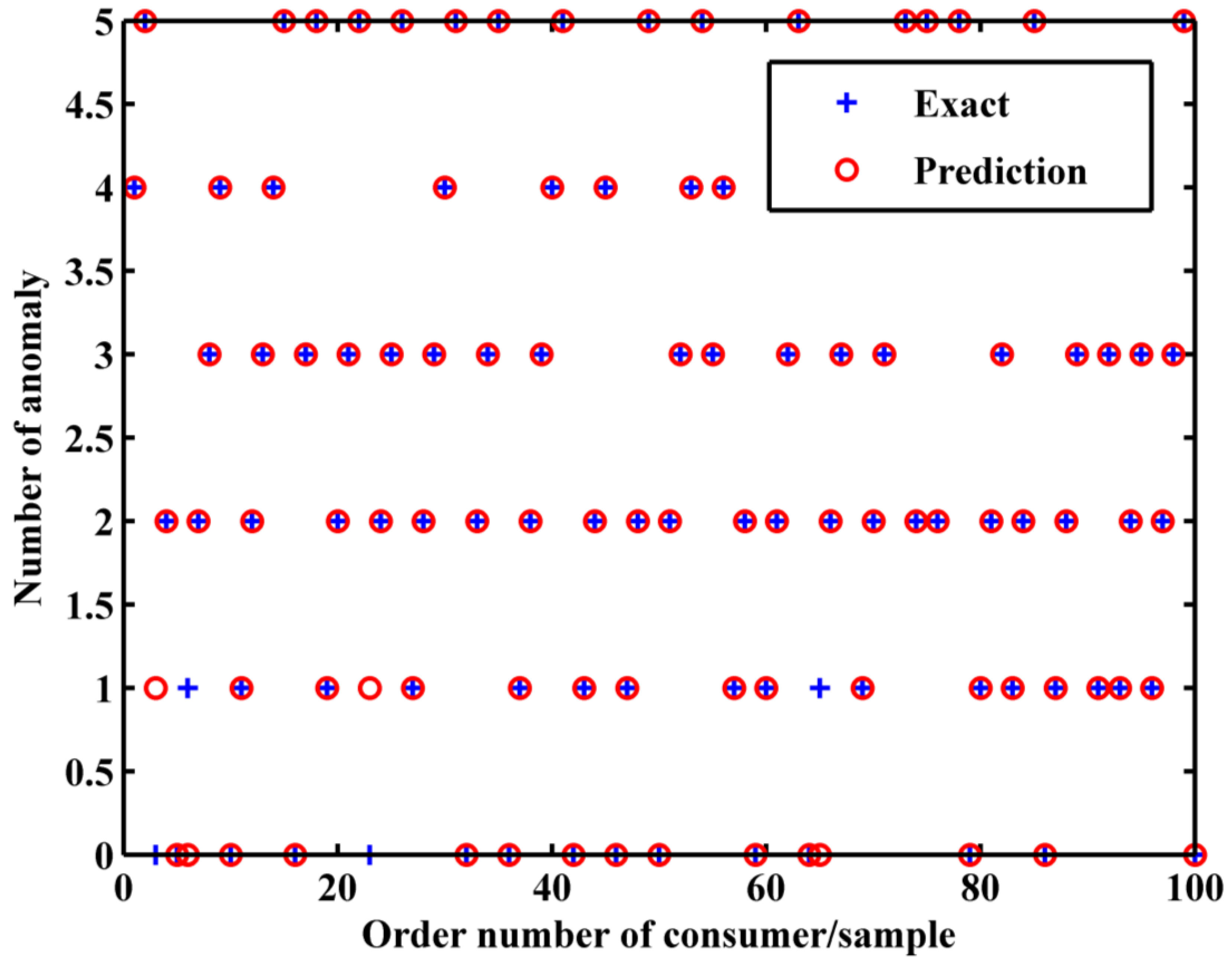
The proposed ANN initially provided the best performance with the smallest frequency error of 10.23%; however, it demanded a significant training time exceeding 600 s. The frequency error, commonly used as a performance evaluation metric for machine learning (ML) algorithms, pertains to the discrepancy in outputs. It is defined as the percentage of mismatches in the detection of anomaly types across the entire dataset. Consequently, an alternative approach was employed. 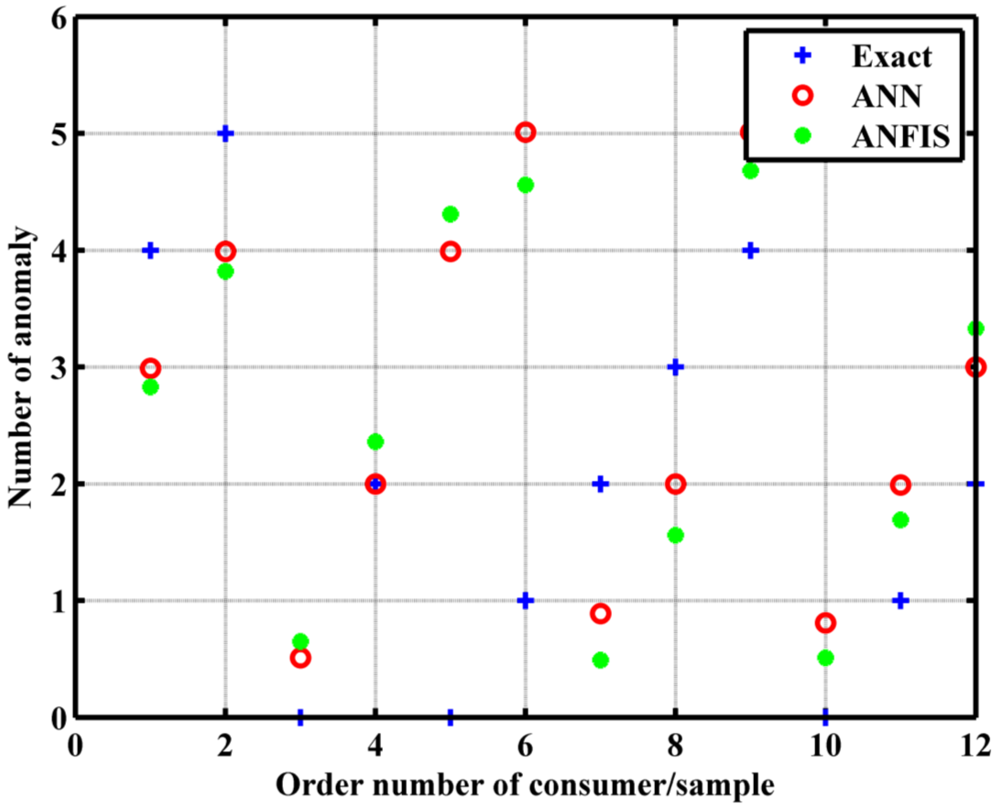In this new design, instead of using the time series of consumption as inputs, statistical indicators derived from the time series, labeled as a₁, a₂, a₃, a₄, a₅, and T, were used. The output, in this case, still predicts the type of anomaly. As expected, this adjustment in input data led to substantially reduced training times less than 10 s. The optimal ANN structure for this configuration includes five layers with the following number of neurons: 60, 30, 10, 10, and 10. The minimum error achieved with this setup is 7.62%. For a visual representation of the testing results under this modified approach, please refer to Figure 4.

Each statistical parameter provides valuable information about the characteristics of the load profile, which can aid in distinguishing between normal load patterns and NTLs. The coefficient of variation (a₁) measures the relative variability of the load profile, providing insight into the consistency or randomness of the load distribution. The ratio between the peak and valley load (a₂) highlights the contrast between the highest and lowest load values, which can be indicative of abnormal usage patterns. The ratio between the peak and average load (a₃) indicates the proportion of the peak load relative to the average load, which can help detect unusual spikes in consumption. The valley coefficient (a₄) quantifies the depth of valleys in the load profile, aiding in identifying periods of low consumption. The load variance (a₅) provides insights into the overall variability of consumption. The time of maximum power utilization (T) identifies the time at which the peak load occurs, which can be crucial for understanding usage patterns. All the coefficients have some limitations in capturing specific patterns within the load profile, but when all six statistical coefficients are used, then the probability that any anomaly will not be noticed decreases. When integrated into AI algorithms, such as the ANN, ANFIS, and K-means clustering, these statistical indicators enhance the algorithms’ ability to detect NTLs by providing them with relevant features that encapsulate different aspects of the load profile. For example, the ANN and ANFIS can learn complex relationships between these statistical parameters and the occurrence of NTLs, while K-means clustering can use these features to cluster load profiles and identify outliers associated with NTLs. However, it is essential to acknowledge that the effectiveness of these statistical indicators depends on various factors such as data quality, feature selection, and the specific characteristics of the NTL being detected.

4. ANFIS

Both ANNs and fuzzy logic systems are capable of regulating nonlinear, dynamic systems that lack a suitable mathematical model. The drawback of the ANN lies in its limited interpretability, particularly in terms of understanding how it tackles management problems. In other words, it lacks transparency in its decision-making process. The ANN does not possess the capacity to generate structural knowledge, such as rules, nor can it leverage pre-existing knowledge to expedite the training process. In contrast, fuzzy expert systems provide transparency in their inferences by employing a set of explicit linguistic rules, typically in the form of “if/then” statements. However, they lack the presence of suitable learning algorithms to adapt and refine their performance based on data from a database.

On the other hand, ANNs do not explicitly define input–output relations through rules but instead encode these relations in their internal parameters, which are learned from the data during training. The integration of ANNs and FL has yielded one of the most successful neuro-fuzzy models known as the ANFIS (adaptive network based fuzzy inference system). The ANFIS leverages both ANNs and FL to create a versatile and widely used hybrid model. It functions as an adaptive network that embodies the principles of fuzzy inference, offering the best of both worlds. A key advantage of the ANFIS is its adaptability, particularly in deriving membership functions from consumption data that characterize the system’s behavior with respect to input–output variables. Unlike traditional fuzzy systems in which manual fuzzification and adjustments of membership functions are required, the ANFIS automatically forms membership functions based on the consumption database. Detailed mathematical formulations of the ANFIS are provided in [17,22]. By utilizing this structure and algorithm, the ANFIS ensures that membership function parameters are not arbitrarily chosen but rather determined from input–output data. These parameters evolve through a learning process facilitated by the gradient vector. The gradient vector gauges how well the fuzzy inference model fits the input–output data for a given parameter set. Optimization methods are then applied to adjust the parameters and minimize the error rate, typically measured as the sum of the squared differences between the actual and desired outputs. The ANFIS employs a hybrid algorithm that combines the backpropagation gradient descent method with the least squares method to facilitate learning. The backpropagation algorithm fine-tunes the parameters of the premise membership functions, while the least squares method adjusts the coefficients of the linear combination in the conclusion. This iterative adjustment process enables the ANFIS to continually refine its model based on training input–output sets, ensuring optimal performance and adaptability in various applications.

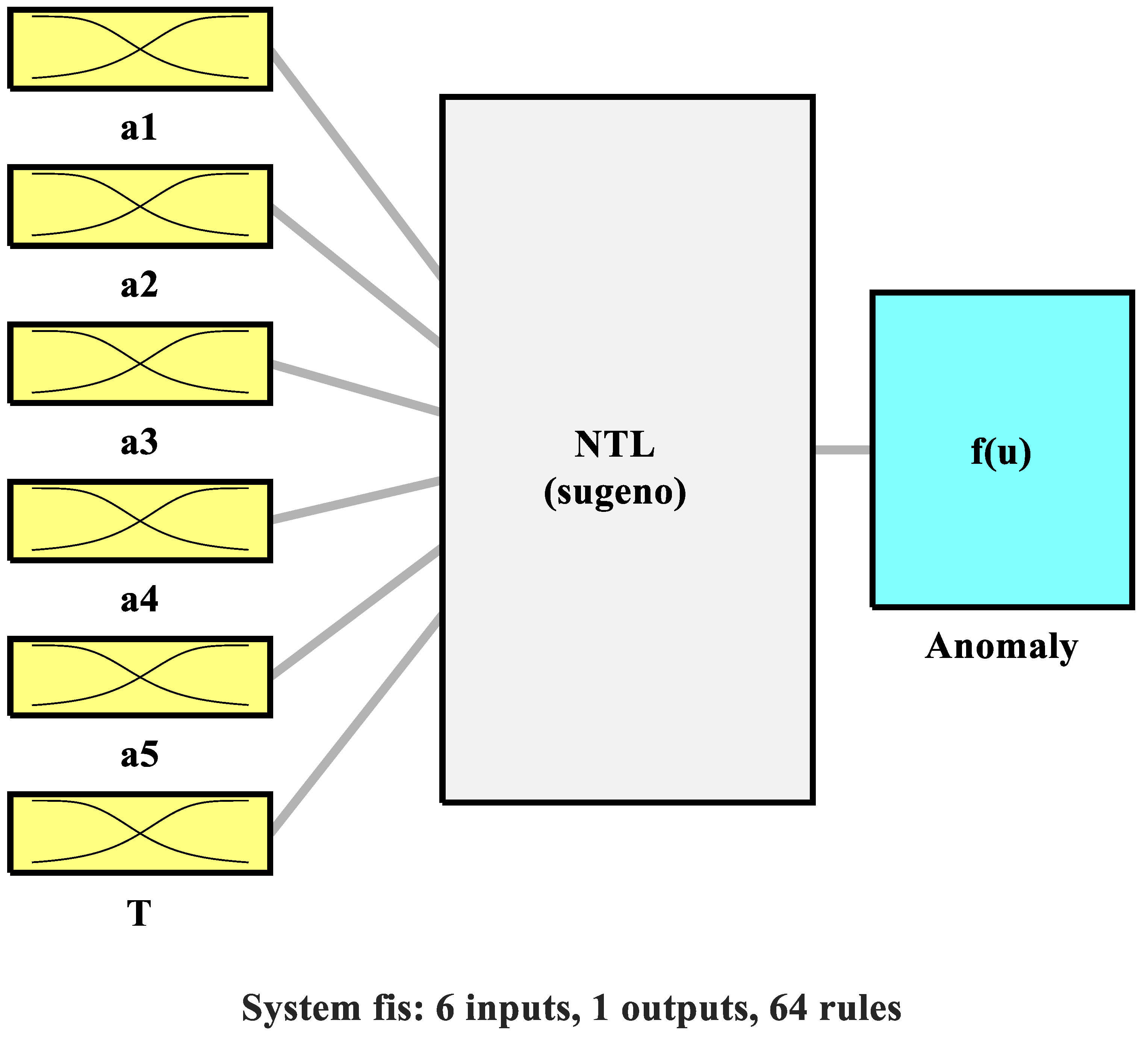
The inputs of the ANFIS are the statistical indicators, while the output is the anomaly number. Therefore, the utilization of the constructed ANFIS will yield a numerical indication, along with the type of anomaly, if an NTL is detected, and will be zero if an NTL is not present. The algorithm of creating the ANFIS is shown in Figure 3. The created ANFIS model is presented in Figure 5. The comparison between the ANFIS and ANN is presented in

Table 3. Mean values of statistical indicators for anomaly detection.

Anomaly	3	4	0	2	4	5	1	2	5	1	2	3
ANN	2.99	3.99	0.51	2.00	3.99	5.01	0.89	2.00	5.01	0.81	1.99	3.00
	3	4	1	2	4	5	1	2	5	1	2	3
ANFIS	2.83	3.82	0.65	2.36	4.31	4.56	0.49	1.56	4.68	0.51	1.69	3.33
	3	4	1	2	4	5	0	2	5	1	2	3

and Figure 6. The minimum ANFIS error reached is 11.11%. Table 3 illustrates that the ANN provides more accurate numerical values for identifying anomaly types, with fewer errors compared to the ANFIS. Specifically, when rounding the numerical values in the table, the ANN makes a mistake in only one instance, whereas the ANFIS errors in two cases within the test set presented in the table. Both the table and Figure 6 collectively suggest that the ANN delivers a superior performance in this context. The ANFIS could improve its performance by obtaining a bigger database and having better data preprocessing. Also, the fuzzy rule base can be reviewed and refined in the ANFIS model to incorporate domain knowledge or insights from experts in electricity consumption patterns.

5. Autoencoder

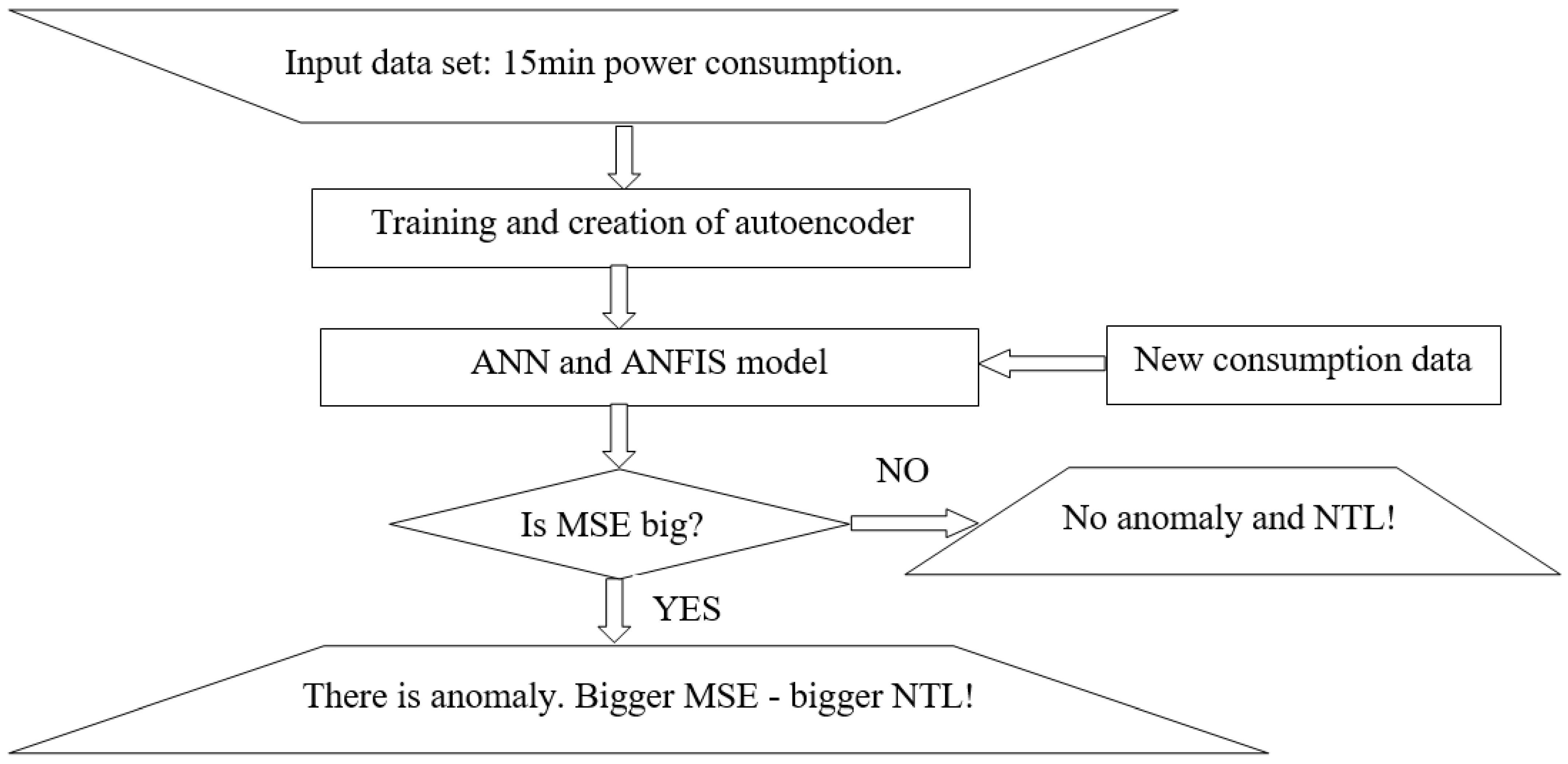
Autoencoder neural networks represent a specific subspecies of ANNs [23,24]. An autoencoder is an unsupervised neural network that, by utilizing an unlabeled dataset, learns an effective method to compress and encode input data. After that, it is trained with the aim of reconstructing an identical data set. An autoencoder consists of two basic elements: an encoder and decoder. The encoder is the part in which the model learns how to compress and reduce the dimensions of the input data, presenting them as encoded information. The decoder is the part in which the model learns how to reconstruct the data from the compressed record as close as possible to the original input data. The part containing the compressed data is often called a “bottleneck” in the literature. After the reconstruction of the input, the reconstruction error is calculated. Various mathematical functions can be used as a tool to estimate error. Similar to the training and validation of ANNs, the calculation of mean square deviations, commonly known as the mean squared error (MSE), is frequently employed. The system’s performance has a direct impact on the faithfulness of the reproduced data. When this error is minimized to a very low percentage, the reproduced output closely resembles the data used during the network’s training phase, approaching a near-identical replication. However, if a larger error is observed for the learned autoencoder during the subsequent processing of a new data set, this data may indicate disturbances in the input data set; that is, they may indicate that there has been a significant change in one of the input parameters. This principle is used to detect anomalies in energy consumption. So, the autoencoder is trained on the data from honest consumers and then the new data are given as the input. If the input data contains an NTL, the MSE tends to be larger than usual, especially when the NTL itself is substantial. A higher MSE indicates a more pronounced anomaly in energy consumption, reflecting an increased deviation from the expected or normal patterns. The input data are the time series of energy consumption. The training time is 77 sec. Ideally, it would be advantageous to have a dataset consisting of honest energy consumers to train the autoencoder. Subsequently, you can input a new time series of measurements into the trained autoencoder and use the mean squared error (MSE) as an indicator. If the MSE is significantly higher than expected, it can serve as an alert for the presence of anomalies in the data, helping to identify potential irregularities in energy consumption. This approach can effectively flag deviations from normal patterns and contribute to anomaly detection. The algorithm is shown in Figure 7, and the results are presented in

Table 4. MSE of autoencoder for different types of anomalies.

Anomaly	No	1	2	3	4	5
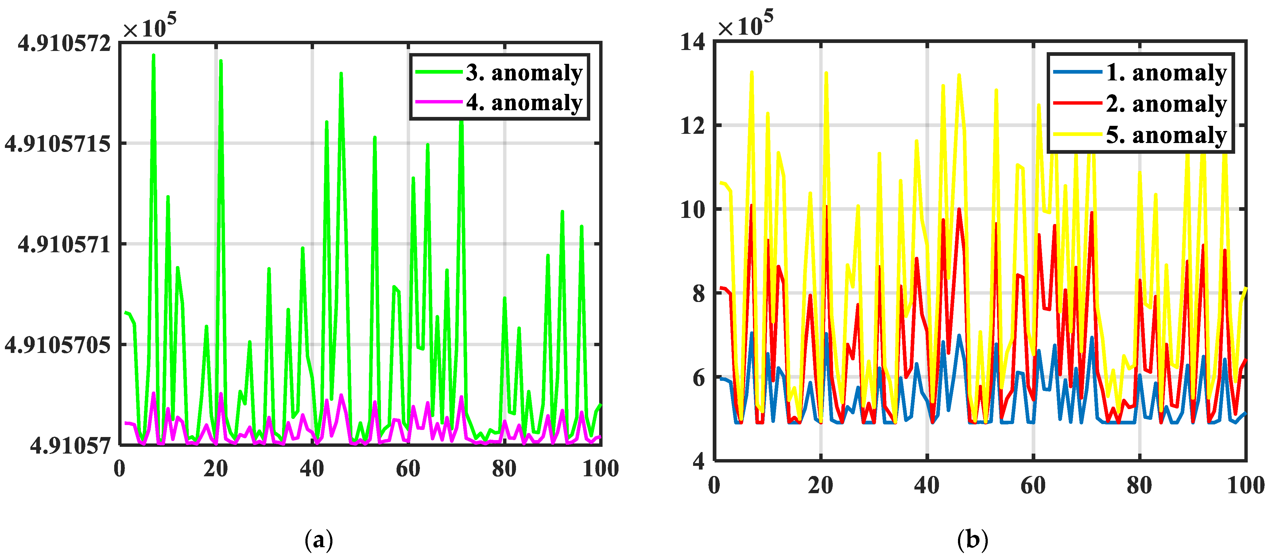
MSE	5.64	4.82 × 104	3.82 × 105	6.92 × 105	9.59 × 105	5.22 × 103

. The autoencoder successfully detects all types of anomalies with significantly higher MSE values. Anomaly type 1 indicates random electricity theft. The MSE is less in the fifth type of anomaly because it only reduces the peak loads. So, the biggest NTLs and MSE values are in anomaly type 4, followed by 3 and 2.

The frequency error is recorded as 0% since the autoencoder consistently identifies anomalies in each case. The mean squared error (MSE) values presented in Table 4 and depicted in Figure 8 affirm the successful detection of NTLs and electricity theft. Additionally, Figure 8 illustrates that there is no clear rule governing how the MSE is directly linked to the type of anomaly. As a result, the application of the autoencoder cannot precisely determine the type of anomaly, but it effectively indicates the magnitude of NTLs and the extent of energy theft.

6. K-Mean

One of the unsupervised ML algorithms that is often used for clustering is the K-mean algorithm. The K-mean algorithm is an optimization technique aimed at categorizing entities into distinct groups [19,25,26]. Each entity is meticulously assigned to a particular cluster, driven by a pursuit of precision. This entails achieving two pivotal cluster attributes: intra-cluster homogeneity and heterogeneity. Homogeneity indicates that the data points exhibit a remarkable degree of resemblance in the same cluster. Heterogeneity indicates disparities among the data points across different clusters and helps in demarcating the boundaries between them. The K-means algorithm provides a valuable perspective for gaining a deeper understanding of the characteristics within each cluster. At the heart of the K-means algorithm lies an iterative process that partitions entities into clusters based on similarity. This cyclic process involves the integration of freshly introduced entities with pre-existing groups. The existing clusters evolve through expansion, absorbing new entities.

In the execution of a cluster analysis, a fundamental aspect is the quantification of the similarity between two entities. This quantification relies on the traits they possess, which are condensed into a measure known as the Euclidean distance, calculated using the following formula:

$$d_E\left(x,y\right)=\Vert x-y\Vert =\sqrt{{{\displaystyle \sum _{i=1}^n\left(x_i-y_i\right)}}^2}=d_E\left(y,x\right)$$

(5)

where x = (x1, …, xn) and y = (y1, …, yn) are attribute values of two objects of length n. In this implementation, x and y are the values of the six above-mentioned statistical indicators. To achieve the optimal performance, cluster algorithms necessitate data normalization to mitigate the disproportionate influence of attributes with larger ranges on the outcomes. As suggested in [27], one of the proposed normalization solutions is min–max normalization, which is defined as follows:

$$x^{*}=\frac{x-\min \left(x\right)}{range\left(x\right)}=\frac{x-\min \left(x\right)}{\max \left(x\right)-\min \left(x\right)}$$

(6)

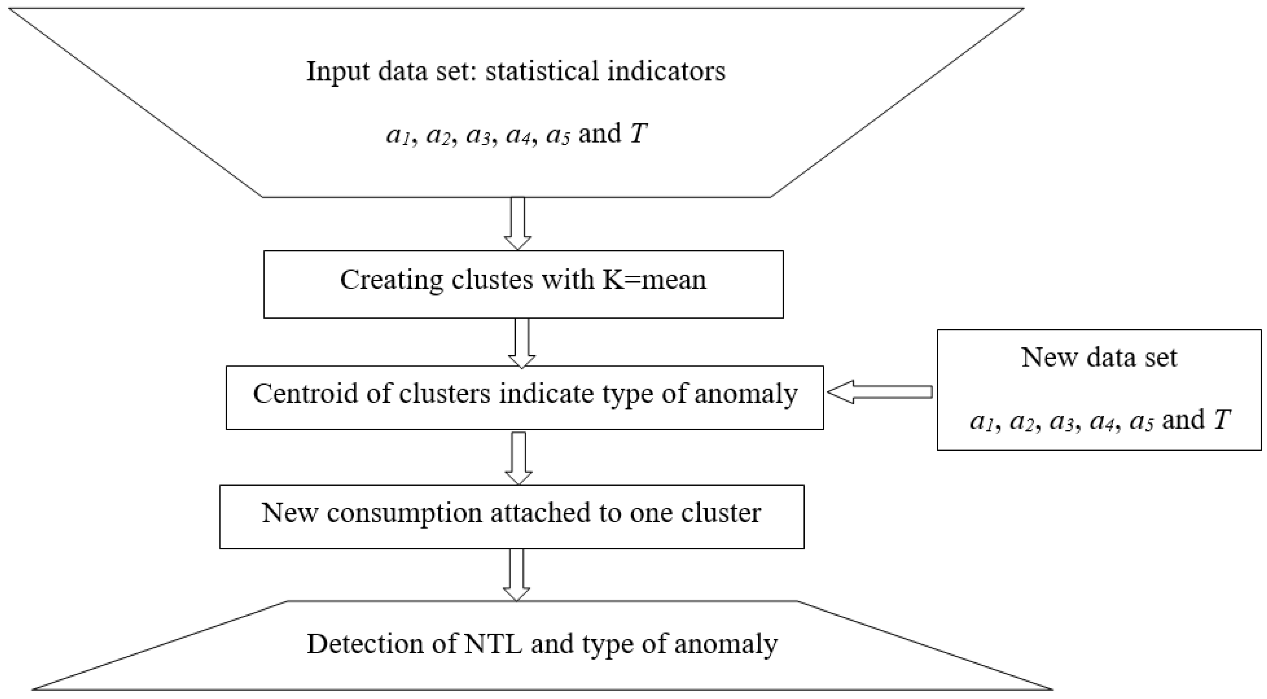
The idea is to use this algorithm on a database of created statistical indicators for different cases of honest consumers and five types of anomalies. The K-mean based on the values of the statistical indicators should divide the consumers into six different clusters in coordination with theft types. The proposed algorithm is depicted in Figure 9. In this context, the new consumption data, which generate a fresh set of statistical indicators, will serve as the new input and be incorporated into one of the existing clusters. Consequently, the methodology will flag NTLs if the new data do not align with the characteristics of the first cluster. The cluster number will provide an indication of the anomaly type, with each cluster center corresponding to a specific anomaly type. This approach leverages clustering to categorize and identify different types of anomalies based on the similarity of statistical indicators.

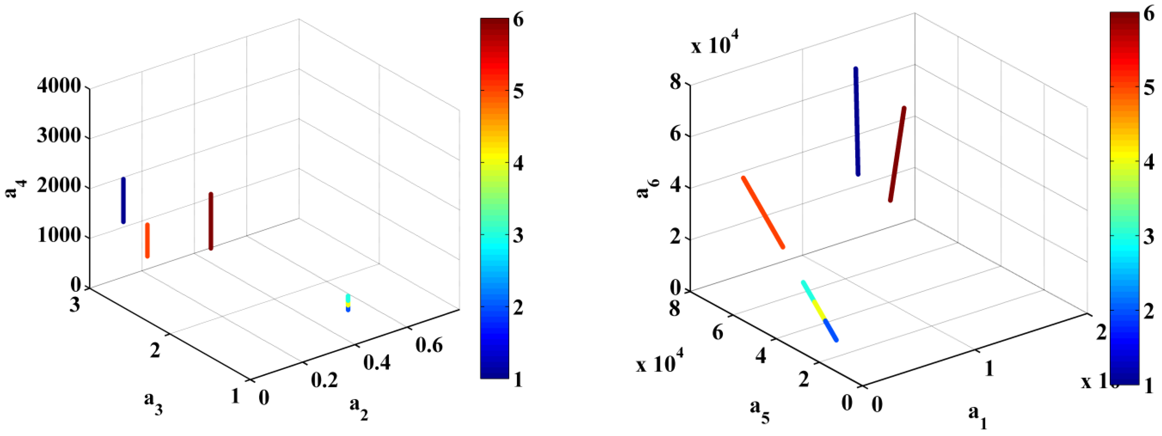
Figure 10 illustrates the clusters within a subspace delineated by three indicators. While this three-dimensional depiction provides a visual understanding, it is crucial to acknowledge that the clusters are delineated within a multidimensional realm. Within this space, each statistical indicator corresponds to one dimension. The points cannot be clearly seen in Figure 10 because they are very close to each other. Upon evaluating the algorithm’s effectiveness through simulations involving the various types of theft, it was observed that the algorithm tends to group honest users together with the fifth anomaly, which corresponds to the sixth group among the clusters. This outcome aligns with our expectations, as the fifth anomaly exhibits the least deviation from the behavior of honest consumers compared to the other anomalies. With a test dataset comprising 6000 samples, the algorithm missed 556 instances, resulting in an error frequency of approximately 9.26%. This finding underscores the algorithm’s ability to identify and differentiate anomalies, even in cases in which they closely resemble honest consumer behavior. With an increased volume of data and consumers, along with a higher occurrence of anomalies and a greater number of typically honest consumers of electrical energy, the K-means algorithm ought to analyze a larger number of clusters.

7. Results and Comparison

A comparison of the five presented methodologies, using an example involving six consumers, is presented in

Table 5. Inputs for testing of methodologies.

Indicators	Honest	1. anom.	2. anom.	3. anom.	4. anom.	5. anom.
a1	53.41	4.37 × 1015	9.12 × 1015	6.41 × 1015	7.56 × 1015	5.61 × 1015
a2	0.0423	0.0356	0	0	0	0.4833
a3	8.47	9.27	22.31	13.66	14.30	9.77
a4	1.51	1.21	1.63	1.20	1.15	1.46
a5	95.66	70.36	76.14	77.66	61.46	85.67
T	109.16	103.67	87.95	70.20	60.44	104.48
Statistical	yes	yes	no	yes	yes	no
ANN	0.33/0	0.86/1	2/2	2.88/3	3.99/4	5.02/5
ANFIS	0.41/0	0.39/0	1.69/2	2.49/3	4.33/4	4.51/5
Autoencoder	5.64	4.82 × 104	3.82 × 105	6.92 × 105	9.59 × 105	5.22 × 103
K-mean	0	2	3	4	5	0

For ANN and ANFIS, the first values show model output and the second values indicate anomalies.

. The inputs consist of measurements from these six different consumers, each of which represent honest consumers, without NTLs, as well as five specific types of energy theft anomalies. All the machine learning methodologies are implemented using the Python programming language, while all the illustrations and images are generated using MATLAB 2023b software. As explained in this paper, only the autoencoder uses the direct time series of energy consumption measurements, while the other methodologies use the statistical indicators as inputs, as they have shown a better performance with them. The output of the autoencoder is the MSE, which indicates the dishonest consumers without error but cannot detect the anomaly type. So, the autoencoder successfully detect all anomalies but cannot detect the type of anomaly. For this example and test scenario, the statistical methodology fails to detect the second and the fifth anomaly, as it does not meet the conditions outlined in the second section of the paper. On the other hand, the ANN successfully identifies all consumer types with a frequency error of 7.62%. The ANFIS misses the first type of anomaly, resulting in a frequency error of 11.11%. The K-means algorithm, however, groups the honest consumers with the fifth anomaly, leading to a frequency error of 9.26%. Both the K-means algorithm and the ANN exhibit similar error rates and are equally effective in detecting NTLs and identifying the type of anomaly. The unsupervised methodology prevails because it does not require knowledge on which consumers are honest and which are not.

Table 6. The comparison of ML algorithms.

ML Algorithm	Frequency Error [%]	Detection of Theft	Detection of Anomaly Type
ANN	7.62	Yes	Yes
ANFIS	11.11	Yes	Yes
Autoencoder	0	Yes	No
K-mean	9.26	Yes	Yes

presents a comparison of the ML algorithms. The disadvantage of all the algorithms, except for the autoencoder, is that they do not utilize direct energy consumption measurements. The other algorithms yield better results when utilizing statistical indicators as inputs, but they require additional processing time for these indicators. However, the autoencoder is limited in its ability to detect the type of dishonest consumer. Among the algorithms, the statistical methodology exhibits the highest frequency error, while the ANFIS fails to detect the first type of anomaly. Both the K-means algorithm and ANN demonstrate superior results in detecting dishonest consumers and their types. One limitation of applying such methodologies is the necessity of an adequate database within the distribution power system. Additionally, the statistical method requires the understanding and reasoning of an energy engineer. For other machine learning methods, mathematical reasoning is essential, yet the described application algorithm allows for straightforward implementation across various programming languages. The robustness of AI algorithms against variations in electricity consumption data characteristics, such as seasonality or changes in consumer behavior, largely depends on the representation of training data and the selection of statistical indicators. If the training dataset adequately captures the diversity of electricity consumption patterns across different seasons and consumer behaviors, the algorithms are likely to exhibit a greater robustness. Including data from various time periods and demographic regions can enhance this aspect. In this paper, we analyze data from 91 consumers with a 15 min interval over one year. However, different resolutions of data and a larger number of consumers will necessitate longer training times but yield more robust AI models.

The selection of statistical indicators plays a crucial role in the performance of AI algorithms because they can effectively capture the nuances of electricity consumption data across seasons and changing consumer behaviors. In this way, AI algorithms will be better equipped to generalize unseen variations. Techniques such as dropout (in neural networks) or rule pruning (in the ANFIS) can help mitigate overfitting and improve the generalization performance. Regularization techniques encourage the model to learn more robust and generalizable representations from the data, making them less sensitive to variations.

K-means clustering might be sensitive to outliers or noisy data. Preprocessing steps such as data scaling or outlier removal can enhance its robustness against such variations. Periodically retraining AI algorithms with updated data can help them adapt to evolving consumption patterns and consumer behaviors, ensuring that the models remain relevant and effective over time, even with the changing characteristics of electricity consumption data.

Combining predictions from multiple AI models trained on different subsets of data or using different algorithms can enhance their robustness. Ensemble methods can help mitigate the weaknesses of individual models and provide more reliable predictions across diverse scenarios.

The larger volume of the distribution power system and its complexity increase the size of the database and the number of consumers that need to be analyzed. The scalability of the proposed AI techniques is crucial for their practical applicability in handling larger datasets. The ANN can be scaled relatively well to handle larger datasets because advancements in hardware, such as parallel processing and distributed training frameworks, have enabled the efficient training of larger neural networks. ANFIS models generally have a simpler structure compared to ANNs, making them more lightweight and potentially easier to scale. Autoencoders are adept at learning compact representations of data, which can be beneficial for handling large datasets by reducing their dimensionality without a significant loss of information. The K-means algorithm is known for its computational complexity, which is linear with the number of data points, making it suitable for large-scale applications.

The K-means algorithm can be parallelized efficiently but is sensitive and may struggle with high-dimensional data or datasets with irregular cluster shapes. Despite their scalability advantages, the presented AI models may encounter challenges with very large and high-dimensional datasets due to limitations in memory, processing resources, and power.

Ultimately, the choice of methodology should align with the database that the distribution system operator (DSO) possesses and the desired format of the results. Each algorithm has its own application and suitability, contingent on one’s specific requirements and objectives.

8. Conclusions

Our comparative analysis of five distinct methodologies for anomaly detection and non-technical loss (NTL) identification reveals a nuanced picture of their strengths and limitations. The main advantage of this paper is its detailed explanation of the application of these methodologies and their limitations in real applications.

While the autoencoder excels in pinpointing dishonest consumers without error, it lacks the ability to specify the type of anomaly. In contrast, the ANN emerges as a robust choice, successfully detecting all consumer types with the smallest frequency error. The ANFIS demonstrates a solid performance but falls short in capturing the first type of anomaly. The K-means algorithm is effective in detecting NTLs, occasionally misclassifying honest consumers with the fifth anomaly. The artificial neural network (ANN) accurately identifies all consumer types with a frequency error of 7.62%, while the K-means algorithm exhibits a slightly higher error rate of 9.26%. However, the ANFIS system fails to detect the initial anomaly type and demonstrates a frequency error of 11.11%. The preference for unsupervised methodologies like K-means and ANN arises from their independence from prior knowledge of consumer honesty. Ultimately, the suitability of these methodologies hinges on the specifics of the DSO’s database and their desired result format, underscoring the need for a tailored approach to anomaly detection in electrical distribution networks.

Our future work will be focused on creating software applications for DSOs and trying to use other AI techniques for the same purpose. In the implementation of AI techniques, existing DSO network management frameworks may require modifications to software platforms, data transmission, and workflow processes. In the future, DSOs need to ensure integration and compatibility with existing systems and protocols. Using software, DSOs can plan on-site inspections to catch dishonest customers.