Comparative Analysis of Ground-Based Solar Irradiance Measurements and Copernicus Satellite Observations

Abstract

Solar irradiance data provided by the Copernicus program are crucial for several scientific, environmental, and energy management applications, but their validation by means of ground-based measurements may be necessary, especially if daily and hourly data resolutions are required. The validation process not only ensures that reliable information is available for solar energy resource planning, power plant performance assessment, and grid integration, but also contributes to the improvement of the Copernicus system itself. Ground-based stations offer site-specific data, allowing for comprehensive assessments of the system’s performance. This work presents a comparative statistical analysis of solar irradiance data provided by the Copernicus system and ground-based measurements on a seasonal basis at three specific Italian reference sites, showing a maximum average relative error of less than 7% for hourly horizontal global irradiance in the irradiance range defined by the IEC 61724-2.

1. Introduction

The validation of solar irradiance data provided by the Copernicus program [1,2] by means of ground-based solar radiation measurements plays a crucial role in ensuring the accuracy and reliability of the solar radiation data used for several scientific, environmental, and energy resource management applications. Moreover, data validation by means of ground-based measurements allows for a comprehensive assessment of the Copernicus system’s performance. Ground-based stations provide localized and site-specific data, capturing the unique characteristics of different regions and climatic conditions. The comparison between Copernicus satellite data and ground-based measurements can allow for an investigation of the parameters affecting the discrepancies in the data and, therefore, can provide relevant information for the development of a potential model. Furthermore, ground-based measurements can be used to validate the algorithms and models employed by the Copernicus system [3]. Algorithms process satellite observations to estimate solar radiation parameters, considering atmospheric conditions, cloud cover, and other variables. By comparing the Copernicus data with ground measurements, the accuracy and reliability of these algorithms can be evaluated, enabling refinement and optimization to achieve a better performance in solar radiation estimation. By integrating ground-based measurements, which have a long history of reliable data collection, with satellite-derived data, a more comprehensive and robust understanding of solar radiation patterns and related variations can be achieved [4,5,6,7,8,9,10].

The IEC 61724-1 international standard for Photovoltaic system performance [11] enables the use of satellite data for global and direct solar irradiance estimations, claiming monthly and yearly uncertainties ranging from less than 1% up to 5%. However, for specific applications, i.e., plant capacity evaluation and anomaly detection, hourly resolutions according to the IEC 61724-2 Standard could be used [12].

In this work, we perform a benchmarking of Copernicus satellite solar irradiance and ground-based solar irradiance data for hourly and daily data with respect to ground-based measurements acquired at Italian sites, considering the solar irradiance limits as defined by the IEC 61724-2 [12].

In Section 2, we will review the investigations and validation models proposed in the scientific literature for satellite solar irradiance systems. Section 3 will define the benchmarking scenarios, including a description of the ground instrumentations, the derived datasets, the adopted methodology, and the results obtained for this paper. The discussion and conclusions are covered in the last two paragraphs, Section 4 and Section 5, respectively.

2. Related Works

Several authors have been validating satellite data with ground-based instrumentation, using simple statistical comparisons and/or developing ad hoc models. In [13], the authors performed a validation study of Direct Normal Irradiance (DNI) provided by the HelioMont algorithm that computes the irradiance with data from the Meteosat Second Generation Enhanced Visible and Infrared Imager (SEVIRI) instrument. The validation procedure involved two European sites, characterized by different environmental conditions: the Plataforma Solar de Almería (PSA) in Southern Spain and the Swiss Baseline Surface Radiation Network (BSRN) of Payerne. The cloud effect was taken into account by means of a cloud modification factor index, CMF, that, similarly to other cloud indexes, normalizes cloud coverage to clear sky conditions. The results show that the quality of the Aerosol Optical Depth (AOD) input data plays an important role, affecting the uncertainty in the DNI estimation. Specifically, using HelioMont original AOD data, mean biases from to 115 W/m² to 145 W/m² were obtained while using Copernicus Atmosphere Monitoring Service (CAMS) AOD; mean biases values ranging from 15 W/m² to 25 W/m² can be observed [14].

In Ref. [15], the scholars performed a validation study of six satellite-derived irradiance products (CAMS-RAD, NSRDB, SARAH-2, SARAH-E, CERES-SYN1deg, and Solcast) and two reanalysis irradiance products (ERA5 and MERRA-2) for hourly GHI. The accuracy of these products was verified against complete records from 57 BSRN stations over a 27-year period (1992–2018). They performed a visual inspection to provide qualitative results and, for quantitative verification, the bias-variance decomposition of Mean Square Error (MSE) was used. The conclusions showed better performances for the two reanalysis irradiance products, ERA5 and MERRA-2. In [16], the authors compared Global Horizontal Irradiance (GHI) and DNI for ground-based observations obtained in Petrolina (northeast Brazil) with the estimates from 11 commonly used solar databases: CAMS, CERES, ERA5, INPE, MERRA-2, Meteonorm, NASA-POWER, NSRDB, SARAH, SWERA-BR, and SWERA-US, considering both hourly and monthly means. For hourly GHI values, RMS differences are observed, ranging from the most accurate (CAMS, 17.3%) to the least accurate (MERRA-2, 38.9%) results. The latter database also exhibits a larger bias (18.7%) compared to CAMS (4%). Larger RMS differences are found for hourly DNI, ranging from 37% (CAMS) to 63.4% (ERA5). All databases display biases above 12%, except for CERES (−1%). Concerning long-term mean-monthly GHI results, biases of less than 1% were obtained with CAMS, CERES, and NASA-POWER, while MERRA-2 tends to overestimate (13%). Larger biases are observed for mean monthly DNI, ranging from CAMS (3%) to Meteonorm (−18.4%). Overall, CAMS stands out as the most consistent solar database for long-term irradiance time series in Petrolina. In [17], a hybrid deep learning approach is proposed for the estimation of hourly GHI irradiance using geostationary satellite observations. This hybrid approach combines a Convolutional Neural Network (CNN) to extract spatial patterns from satellite imagery and a Multi-Layer Perceptron (MLP) to connect these abstract patterns with additional time and location information, ultimately predicting the hourly global solar radiation. The key advantage of this approach lies in its ability to effectively capture the ever-changing cloud morphology and model complex nonlinear relationships. The deep network is trained using ground-measured radiation data from 90 Chinese radiation stations in the year 2008, along with radiative transfer model simulations at the top of Mount Everest. The trained network is validated at five independent stations in 2008, achieving an overall R² coefficient of 0.82. Comparative experiments confirm that combining spatial patterns with point-specific information leads to more accurate estimations of hourly global solar radiation. This approach can achieve a minimum RMSE of 84.18 W/m², an MBE of −0.12 W/m², and an R² of 0.90. In [18], an optimized Artificial Neural Network (ANN) model was developed to estimate daily GHI using Meteosat satellite images. Differently from other models, information from the infrared channels of Meteosat 9 was used in this case. Each channel provides different information concerning cloud detection, water vapor, and wind, as further detailed in Appendix B. Specifically, the eleven Meteosat-9 channels with 3 km nadir spatial resolution (approximately 4.5 Km in the analyzed site in Andalusia, Spain), were used as ANN inputs. The model was validated from January 2008 to December 2008. Data collected from 83 monitoring stations deployed throughout the region were used, with 65 stations for model training and 18 independent stations for the testing. The results show an RMSE of between 4% and 9% for daily GHI estimation (RMSE = 6.74% at independent stations). In [19], a Deep Neural Network (DNN) was employed to estimate daily GHI for 34 monitoring stations in Turkey. Different input data were used for DNN: astronomical factors, extraterrestrial radiation and climate variables, sunshine duration, cloud cover, and training and testing datasets generated between 2001 and 2007. The results show an R² of 0.98, an MSE of 0.78 MJm⁻² day⁻¹, and an MAE of 0.61 MJm⁻² day⁻¹, suggesting that the employed method can be used as a more general solution. In [20], a satellite-based model was used to estimate the monthly average of daily GHI in Cambodia. The model used long-term ground-based meteorological data and satellite data from June 1995 to December 2008, taking into account the reflection of clouds, absorption and scattering of solar radiation due to aerosols, ozone, water vapor, and gases. The model also estimated earth-atmospheric reflectivity and ground albedo using satellite data. Validation showed good agreement with the ground data, with a root mean square difference limited to 6.3%. Several studies related to the statistical comparison between ground solar irradiance and satellite models were proposed in the last few years. In [21,22], the authors performed a comparison between ground-based monthly GHI and DNI with the satellite-based model SUNY. Ground-based stations are located at the University of Engineering and Technology of Peshawar (Pakistan). Results obtained using satellite data from 2000 to 2014 and ground measurements in 2017 indicated a maximum difference of 42.90% between ground- and satellite-based GHI in December, with a minimum of −3.83% in March. Ground-based GHI was overestimated in February, March, and April, while satellite values exceeded ground measurements in other months. Similarly, a maximum 55.86% difference in DNI was observed in November, with a minimum of −3.34% in March. Satellite-based DNI was underestimated in February, March, and April, and overestimated in other months compared to ground measurements. Correlation analysis revealed R² values of 0.8852 for GHI and 0.4139 for DNI. In [23], the authors proposed a model for estimating monthly GHI, combining the Angstrom–Prescott model and Garcia model, and compared the GHI model’s estimations with ground measurements and satellite data. Ground-based data from three sources in the northwestern region of Nigeria (Sokoto, Kaduna, Kano) and meteorological data from Nigerian Meteorological Agency and NASA were used. The proposed model showed higher accuracy, with RMSE values of 0.376 for Sokoto, 0.463 for Kaduna, and 0.449 for Kano, and higher R² values (0.922, 0.938, and 0.961 for Sokoto, Kano, and Kaduna, respectively). The proposed model showed a better fit with ground measurements than satellite-derived data. In [24], reanalysis data, satellite data, radiation maps generated by statistical methods, and ground measurements were compared for daily GHI observations. The GHI from the reanalysis dataset provided by the ECMWF and the second-generation Meteosat-derived dataset provided by the LSA-SAF were evaluated. These were compared with radiation maps generated by statistical methods and with ground measurements from the National University of Salta (Salta, Argentina). The comparison results showed that the best fit with the ground measurements was obtained using LSA-SAF data (MBE of 8.73 W/m², RMSE of 79.17 W/m², rMBE of 4.2%, and rRMSE of 20%). Another comparison, of Italian sites [25], evaluated GHI estimates from Meteosat Second Generation and another from the one-day forecast of the Regional Atmospheric Modeling System (RAMS) mesoscale model. The ground-based measurements spanned twelve different climatic areas in Italy and one yearlong dataset. The results indicate a dependence on sky conditions, with RMSE increasing from clear to cloudy conditions. Alpine stations exhibit a higher RMSE due to the observed inadequacies in representing cloud coverage. RAMS tends to over-forecast GHI, as shown by the MBE, while MSG-GHI shows no specific behavior. Yearly statistics for RAMS-GHI RMSE range from 152 W/m² (31%) for Cozzo Spadaro (a maritime station) to 287 W/m² (82%) for Aosta (Alpine site). For MSG-GHI, the minimum RMSE is 71 Wm⁻² (14%) for Cozzo Spadaro and the maximum is 181 W/m² (51%) for Aosta. Daily integrated GHI evaluation exhibits a lower RMSE compared to the hourly GHI for both RAMS-GHI and MSG-GHI. The application of model output statistics (MOS) as a post-processing technique improves the RAMS-GHI forecast. A study performed in Greece [26] evaluated solar radiation component estimates from the Meteorological Radiation Model (MRM), satellite-based datasets (CAMS, PVGIS-CMSAF-SARAH), and reanalysis (PVGIS-ERA5) compared to ground measurements at Methoni station. MRM exhibited satisfactory simulations for global solar irradiation at 15 min intervals (R² = 0.97, RMSE = 11.5%, MBE = −2.5%), but larger biases for diffuse radiation, with R² = 0.57 and RMSE = 45%. CAMS estimates showed RMSE values of 19.5%, 38%, and 28% for global, diffuse, and direct radiations at 15 min intervals, respectively, increasing with increasing time intervals. In spite of the fact that PVGIS is not conceived for instantaneous measurement evaluations, the authors conclude that PVGIS databases perform well for global irradiance (R² = 0.82–0.92) but show higher uncertainties for diffuse (R² = 0.39–0.49) and direct (R² = 0.75–0.87) radiation under instantaneous measurements. Clear sky conditions lead to significant improvements in all components, while uncertainties increase in overcast or partly cloudy conditions due to cloud detection limitations. In [27] the authors analyze and compare daily and yearly solar irradiation data from the CM SAF satellite database [28] and 301 stations in the Spanish SIAR network. The analysis estimates effective irradiation on fixed, two-axis tracking, and north–south horizontal axis tilted planes using data from both sources. Additionally, a new map of yearly irradiance values for horizontal and inclined planes is generated using geostatistical techniques (kriging with external drift (KED)). The results show a Mean Absolute Difference (MAD) between CM SAF and SIAR of about 4% for horizontal plane irradiance and between 5% and 6% for irradiance incident on the tilted planes. For the comparison between KED and SIAR, and KED and CM SAF, the MAD is about 3% for horizontal plane irradiance and between 3% and 4% for the irradiance incident on inclined planes. Finally, it is worth recalling that a comprehensive review of solar irradiance evaluations from satellite data can be found in [29].

3. Materials and Methods

In this work, data validation was performed using a comparative approach between ground-based solar radiation data and those provided by the Copernicus system. The methodology used here takes advantage of solar irradiance data collected from three Italian ground-based reference monitoring stations, located, respectively, in the Italian National Agency for New Technologies, Energy and Sustainable Economic Development (ENEA) Research Center of Portici (Napoli), in the ENEA Research Center of Casaccia (Roma) and in the Research Energy System (RSE) center of Piacenza. The solar radiation data used for comparison were obtained by the Copernicus system. The reference stations used in this work were selected to cover representative areas and different climatic conditions. The ground-based solar radiation sensors were calibrated according to international standards to ensure the accuracy and reliability of measurements.

Table 1. Solar irradiance instrumentation deployed in the three analyzed sites and the corresponding measured parameters. The reference stations are all equipped with Class A instrumentations whose precision, range, etc., are defined according to the ISO9060:2018 standard [30]. For instance, as far as pyranometers and pyrheliometers are concerned (the most relevant ground instruments for this experimental work), daily uncertainties of less than 3% and 2%, respectively, are warranted.

Site	Instrument	Measured Parameter	Specifications
ENEA Portici	Solar Tracker EKO mod. STR-22 with Shadow Ball MB 12	Two-Axis Sun Tracker	Pointing accuracy 0 to 87° < 0.01° Angle resolution 0.009°
	Pyrheliometer HUKSEFLUX DR01-10	Direct Irradiance	ISO9060:2018 Class A
	High Precision Pyranometer EKO mod. MS-802F	Global Horizontal Irradiance	ISO9060:2018 Class A
	High Precision Pyranometer EKO mod. MS-802F	Diffuse Irradiance	ISO9060:2018 Class A
	High Precision Pyranometer EKO mod. MS-802F	Global Normal Irradiance	ISO9060:2018 Class A
	High Precision Pyranometer EKO mod. MS-802F	Global Irradiance 30° South	ISO9060:2018 Class A
ENEA Casaccia	Sun Tracker Eko model STR-21	Two-Axis Sun Tracker	Pointing accuracy 0 to 87° < 0.01° Angle Resolution 0.009°
	Pyranometer Eko model MS-802	Global Horizontal Irradiance	ISO9060:2018 Class A
	Pyrheliometer Eko model MS-54	Direct Irradiance	ISO9060:2018 First Class
RSE Piacenza	Eppley PSP-type Pyranometer	Global Normal Irradiance	ISO9060:2018 Class A
	Eplab NIP Pyrheliometer	Direct Normal Irradiance	ISO9060:2018 First Class
	Kipp and Zonen Pyranometer CMP series	Global Horizontal Irradiance	ISO9060:2018 Class B
	Spectrafy SolarSM-D2	Direct Normal Spectral Irradiance	ISO9060:2018 Class A

shows the ground instrumentations for the three analyzed sites and the measured parameters. Data were taken at a 1 min rate and then the hourly and daily averages were calculated.

Ground-based instruments provide measurements of DNI, GHI, and diffuse radiation, together with weather data (temperature, relative humidity, atmospheric pressure, rain, wind speed, wind direction, albedo, and solar elevation angle values). The ground instrumentation dataset, for each site, was synchronized with the corresponding Copernicus dataset, and then the hourly and daily averages evaluated in this paper were computed.

Solar irradiance satellite data were downloaded by the CAMS service, which provides time series of global, direct and diffuse irradiations on a horizontal surface, as well as DNI for the actual weather conditions and clear-sky conditions. The geographical coverage was the field-of-view of the Meteosat satellite, that is, Europe, Africa, Atlantic Ocean, and the Middle East (from −66° to 66° in both latitudes and longitudes). The timeframe coverage ranged from the 1st February 2004 up to the day before the data downloading. Data were available with a time step ranging from 1 min to 1 month [14]. Specifically, after entering the geographical coordinates for a selected location, the system returns its global, beam, and diffuse irradiations integrated over a selected time step (Meteosat Second Generation satellite coverage) and a selected period (see

Table 2. Parameters as provided by the CAMS Radiation Service v4.5 all-sky irradiation (obtained from satellite data) [14].

Parameter	Reference/Measurement Unit
Observation period	ISO 8601 [31]
TOA (irradiation on horizontal plane at the top of atmosphere)	Wh/m2
Clear sky GHI (clear sky global irradiation on horizontal plane at ground level)	Wh/m2
Clear sky BHI (clear sky beam irradiation on horizontal plane at ground level)	Wh/m2
Clear sky DHI (clear sky diffuse irradiation on horizontal plane at ground level)	Wh/m2
Clear sky BNI (clear sky beam irradiation on mobile plane following the sun at normal incidence)	Wh/m2
GHI (global irradiation on horizontal plane at ground level)	Wh/m2
BHI (beam irradiation on horizontal plane at ground level)	Wh/m2
DHI (diffuse irradiation on horizontal plane at ground level)	Wh/m2
BNI (beam irradiation on mobile plane following the sun at normal incidence)	Wh/m2
Reliability (proportion of reliable data in the summarization)	(0–1) Rel = 0 (unreliable data); Rel = 1 (reliable data)

). For one-minute resolution data, it is also possible to include detailed information on atmosphere air quality [14].

Whenever used, the extraterrestrial radiation data used for the computation of the Clearness Index Kt, defined as the ratio of the horizontal global irradiance to the corresponding irradiance available outside of the atmosphere (i.e., the extraterrestrial irradiance multiplied by the sinus of the sun height), were downloaded from the NREL’s Solpos Calculator system [32].

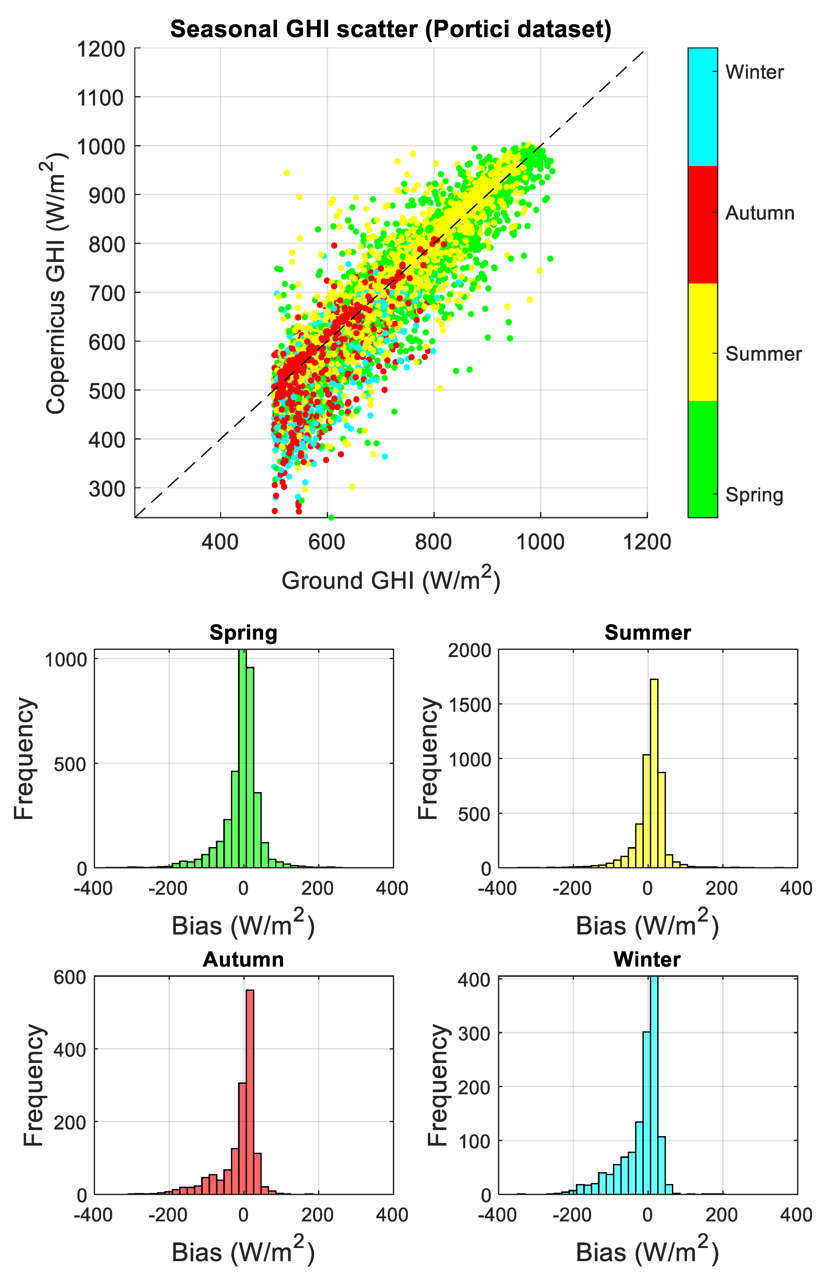
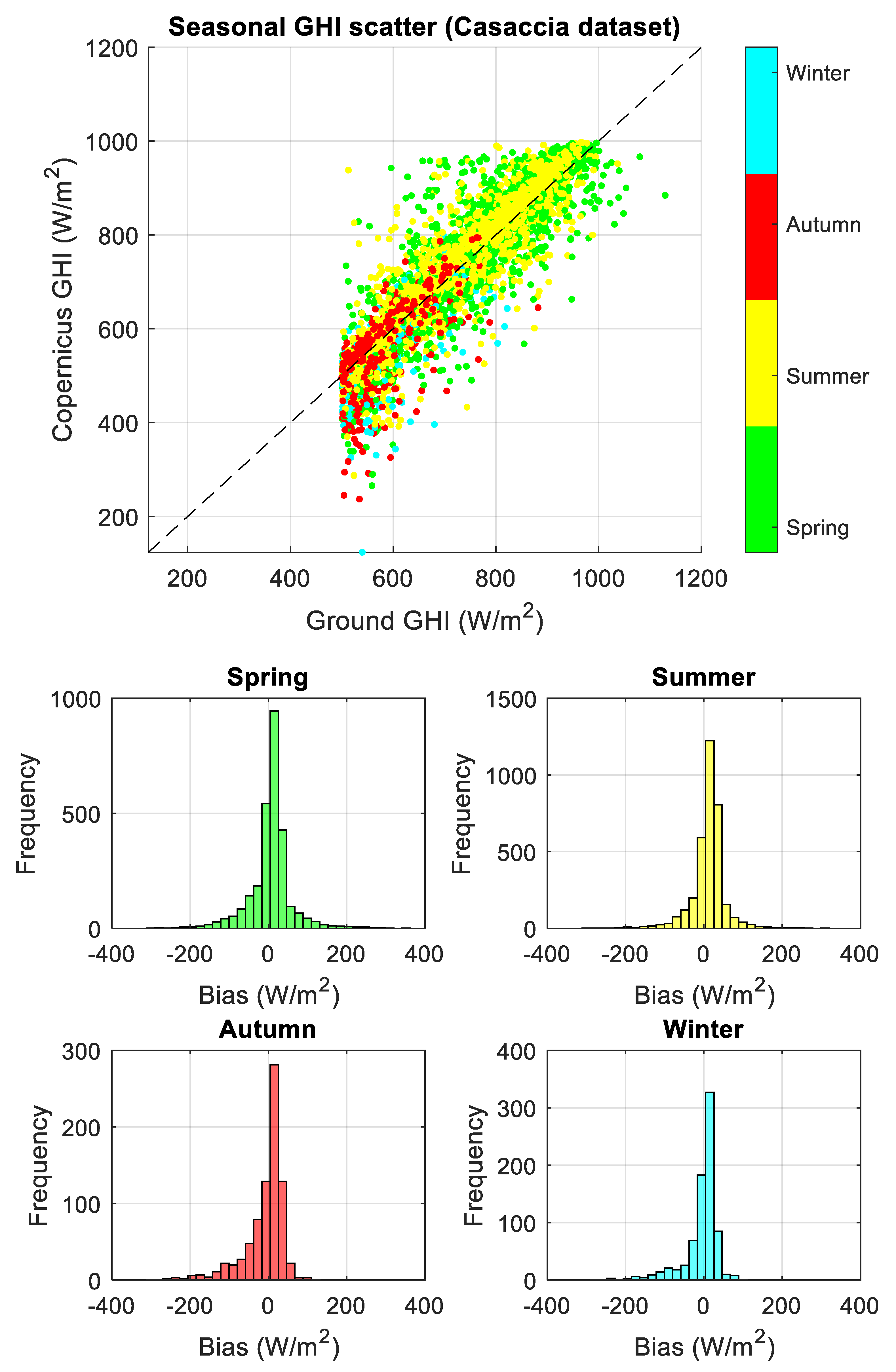
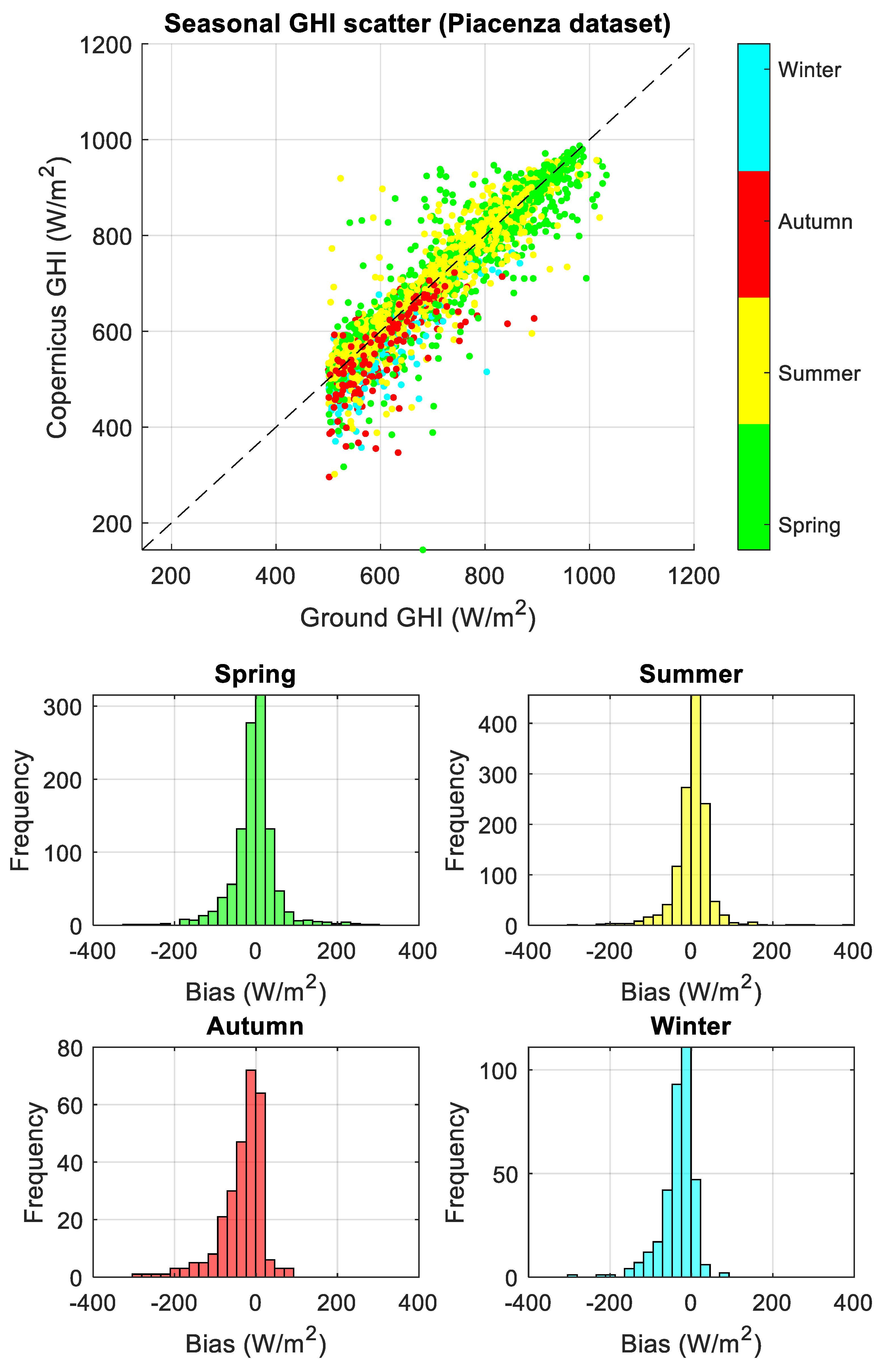
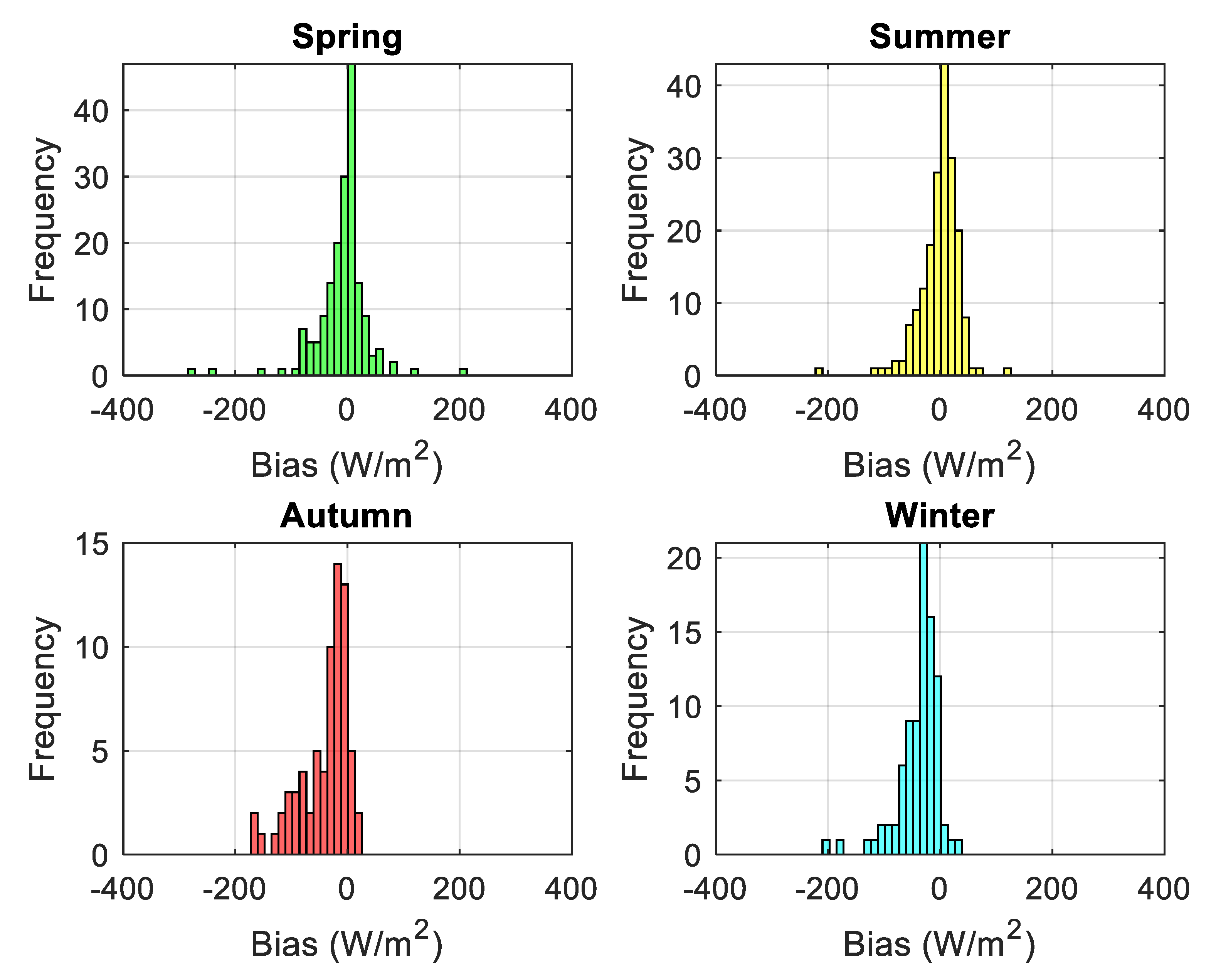
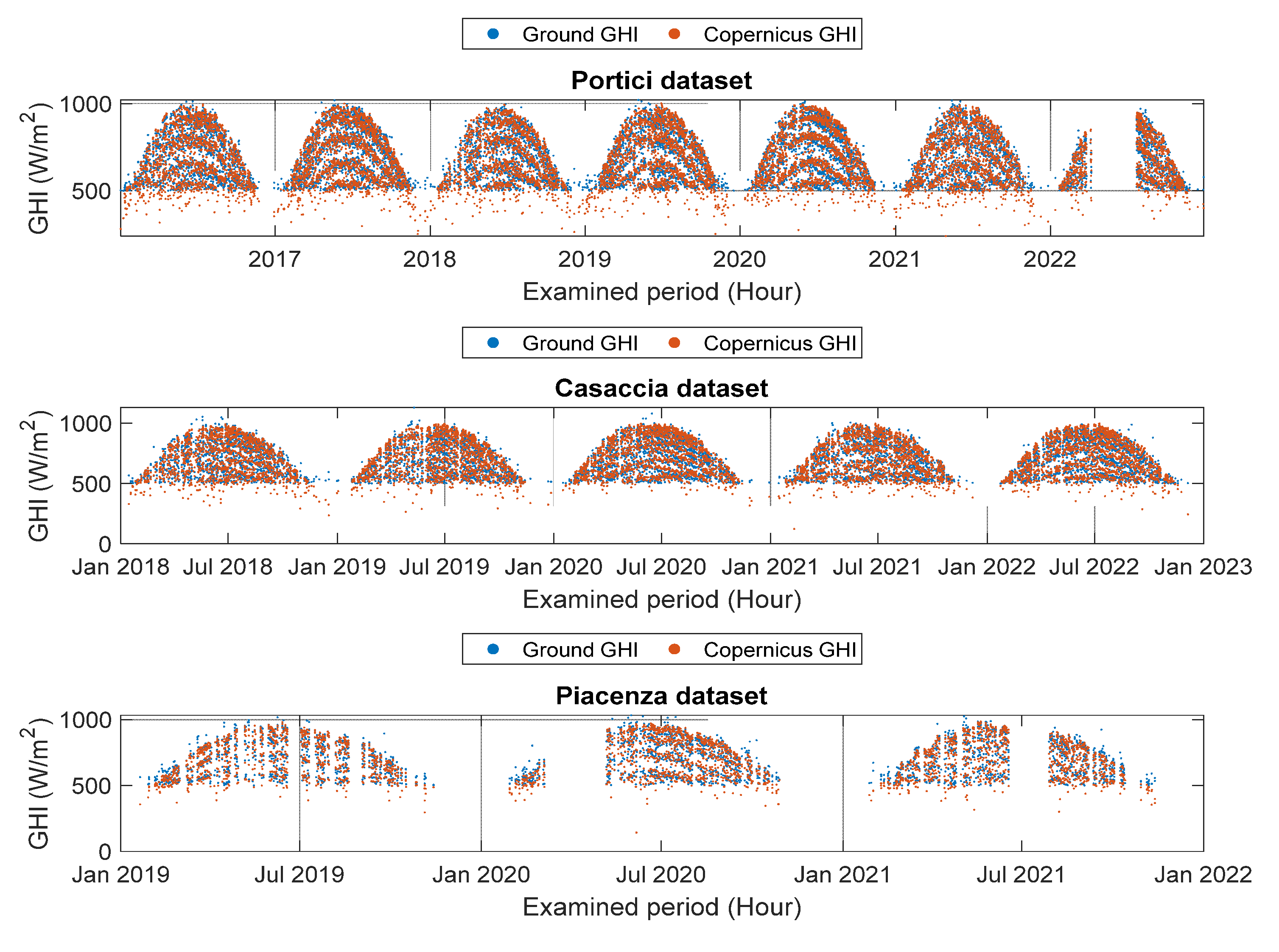
3.1. Comparative Analysis of Hourly Averaged Data

In this paper, satellite vs. ground data were only compared in terms of radiation values in the range from 500 W/m² to 1200 W/m², following the specifications defined in IEC TS 61724-2 [12]. The three filtered datasets were processed as described above, and a statistical comparison was performed on a seasonal basis and is reported in

Table 3. Mean Relative Error and R² metrics computed for seasonal GHI_cop and GHI_ground for the three hourly averaged datasets.

	Season	Num. Samples	MRE	R2
Portici dataset	Spring	3717	4.42%	0.89
	Summer	4761	3.97%	0.91
	Autumn	1438	5.75%	0.65
	Winter	1320	6.23%	0.64
Casaccia dataset	Spring	2783	5.04%	0.86
	Summer	3444	4.42%	0.89
	Autumn	801	6.05%	0.61
	Winter	790	4.75%	0.69
Piacenza dataset	Spring	1101	5.02%	0.84
	Summer	1269	4.14%	0.88
	Autumn	274	6.85%	0.46
	Winter	344	6.24%	0.61

which provides an hourly comparison. Although several different metrics (Appendix A—

Table A1. Performance indicators computed using hourly and daily averaged data (x is the Copernicus GHI vector and y is the ground-based GHI vector.

Comparison Metrics	Short Name	Mathematical Formulas	Characteristics
Absolute Error	AE	$\left|x_i-y_i\right|$	Absolute values of the difference between Copernicus GHI and ground GHI
Mean Bias Error	MBE	$\frac{1}{n}{\displaystyle {\displaystyle \sum }_{i=1}^n}\left(x_i-y_i\right)$	Estimation of the magnitude of differences between Copernicus GHI values and ground-based GHI, averaged over the whole sampling period.
Mean Absolute Error	MAE	$\frac{1}{n}{\displaystyle {\displaystyle \sum }_{i=1}^n}\left|x_i-y_i\right|$	Indicates the average of the magnitude of absolute errors; it does not indicate the direction of the error, but only its magnitude and its sensitive to outliers.
Mean Relative Error	MRE	$\frac{1}{n}{\displaystyle {\displaystyle \sum }_{i=1}^n}\frac{\left|x_i-y_i\right|}{\left|x_i\right|}$	Indicates the average of the magnitude of relative errors; it expresses the average percentage difference between Copernicus GHI values and ground-based GHI.
Root Mean Square Error	RMSE	$\sqrt{\frac{1}{n}{\displaystyle {\displaystyle \sum }_{i=1}^n}{\left(x_i-y_i\right)}^2}$	Indicates the magnitude of the error and retains the variable’s unit; it is sensitive to outliers and extreme values.
Correlation Coefficient	R	$\frac{{{\displaystyle \sum }}_{i=1}^{n }\left(x_i-\overline{x}\right)\left(y_i-\overline{y}\right)}{\sqrt{{{\displaystyle \sum }}_{i=1}^{n }{\left(x_i-\overline{x}\right)}^2{\left(y_i-\overline{y}\right)}^2}}$	Measures the strength and the direction of the linear relationship between two variables and receives a value between −1 and 1; it is independent of the difference in the variance (var) of x and y. Thus, if r = 1 and var(x) < var(y), then a variance correction may be required.
Coefficient of Determination	R2	$1-\left(\frac{{{\displaystyle \sum }}_{i=1}^n{\left(x_i-y_i\right)}^2}{{{\displaystyle \sum }}_{i=1}^n{\left(x_i-\overline{x}\right)}^2}\right)$	Measures the proportion of variance in the dependent variable that can be explained by variations in the independent variable through a regression model. It takes values between 0 and 1, indicating a poor and strong ability of the model to explain variation, respectively. R2 = 1 suggests that the model explains all the variation, while R2 = 0 indicates that the model explains none.

) were finally computed, for the sake of simplicity, Table 3 only reports MRE estimations. To provide a graphical overview of overestimation and underestimation scenarios, the seasonal scatter plots of Copernicus, GHI_cop versus ground, and GHI_ground were derived for the three analyzed datasets, together with seasonal bias error distributions (Appendix A—Figure A1, Figure A2 and Figure A3) and are reported in Figure 1.

Figure A1, Figure A2 and Figure A3 (Appendix A) show that Copernicus data values mainly underestimate ground-based irradiance in the winter and autumn, while the opposite behavior is observed in the spring and summer.

In Table 3, the hourly mean relative error and R² metrics, computed on a seasonal basis, are reported for the three hourly averaged datasets.

After evaluating the absolute error as reported in Abbreviations Section, an acceptance threshold was defined for each season according to Equation (1):

$$threshold=2\times std\left(absolute\_error\right),$$

(1)

The computed thresholds values for each season are reported in

Table 4. Threshold values for the absolute error evaluation. The reported values were computed for each season for the three hourly averaged datasets.

Thresold Values per Season (W/m2)
Site	Spring	Summer	Autumn	Winter
Portici	77.74	64.97	85.07	89.34
Casaccia	85.47	67.67	82.35	77.60
Piacenza	88.76	67.68	95.55	73.27

.

Table 5. Number of occurrences in which the absolute error values exceed threshold values with respect to the total number of events for each season and for the three hourly averaged datasets.

Number of Events Where the Hourly Absolute Errors Exceed the Computed Threshold Value per Season
Site	Spring	Summer	Autumn	Winter
Portici	359/3717 = 10%	366/4761 = 8%	158/1438 = 11%	160/1320 = 12%
Casaccia	291/2783 = 10%	314/3444 = 9%	82/801 = 10%	68/790 = 9%
Piacenza	97/1101 = 9%	98/1269 = 7%	27/274 = 10%	42/344 = 12%

reports the number of occurrences in which the absolute error exceeds the threshold values with respect to the total number of samples for each season and for the three hourly averaged datasets.

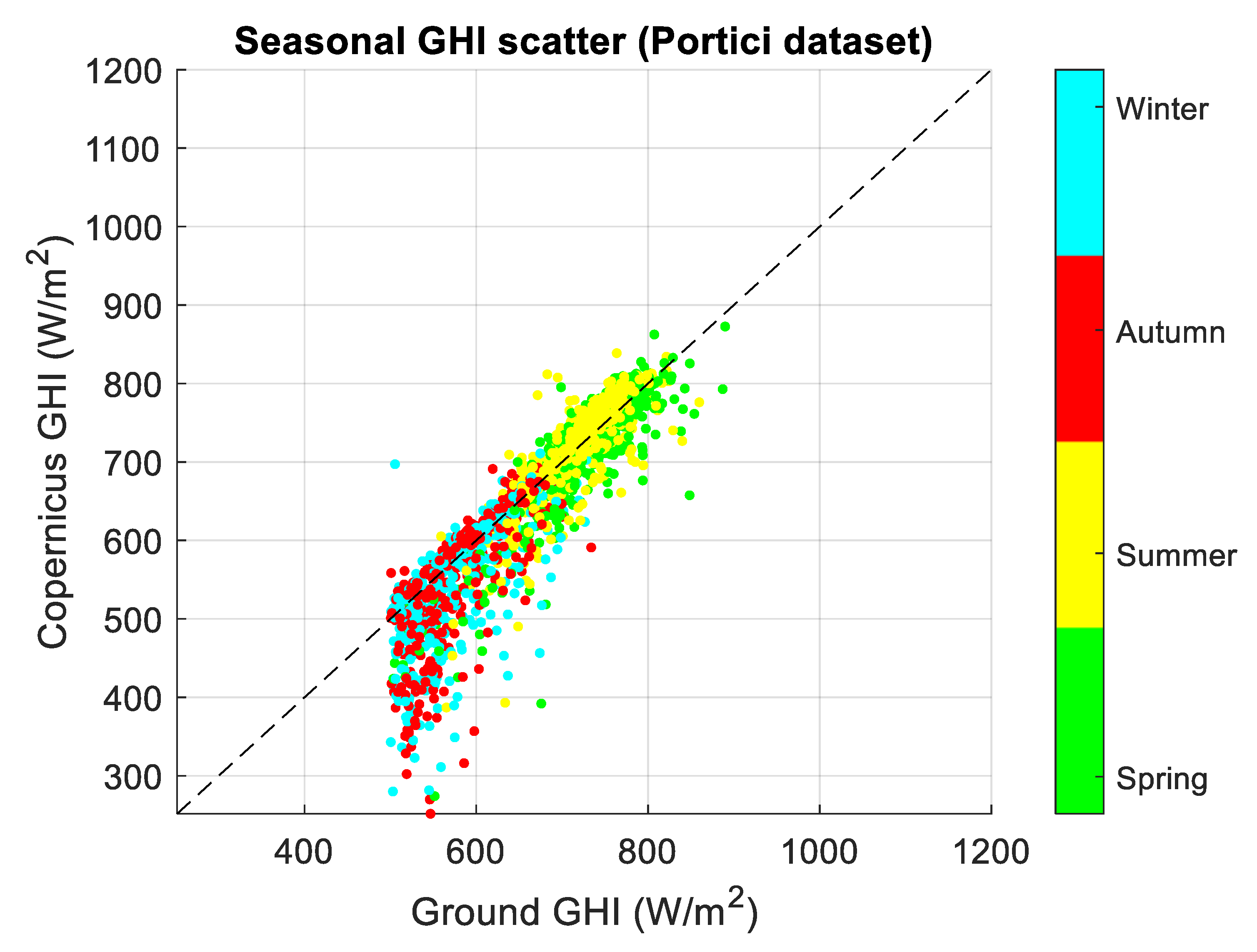
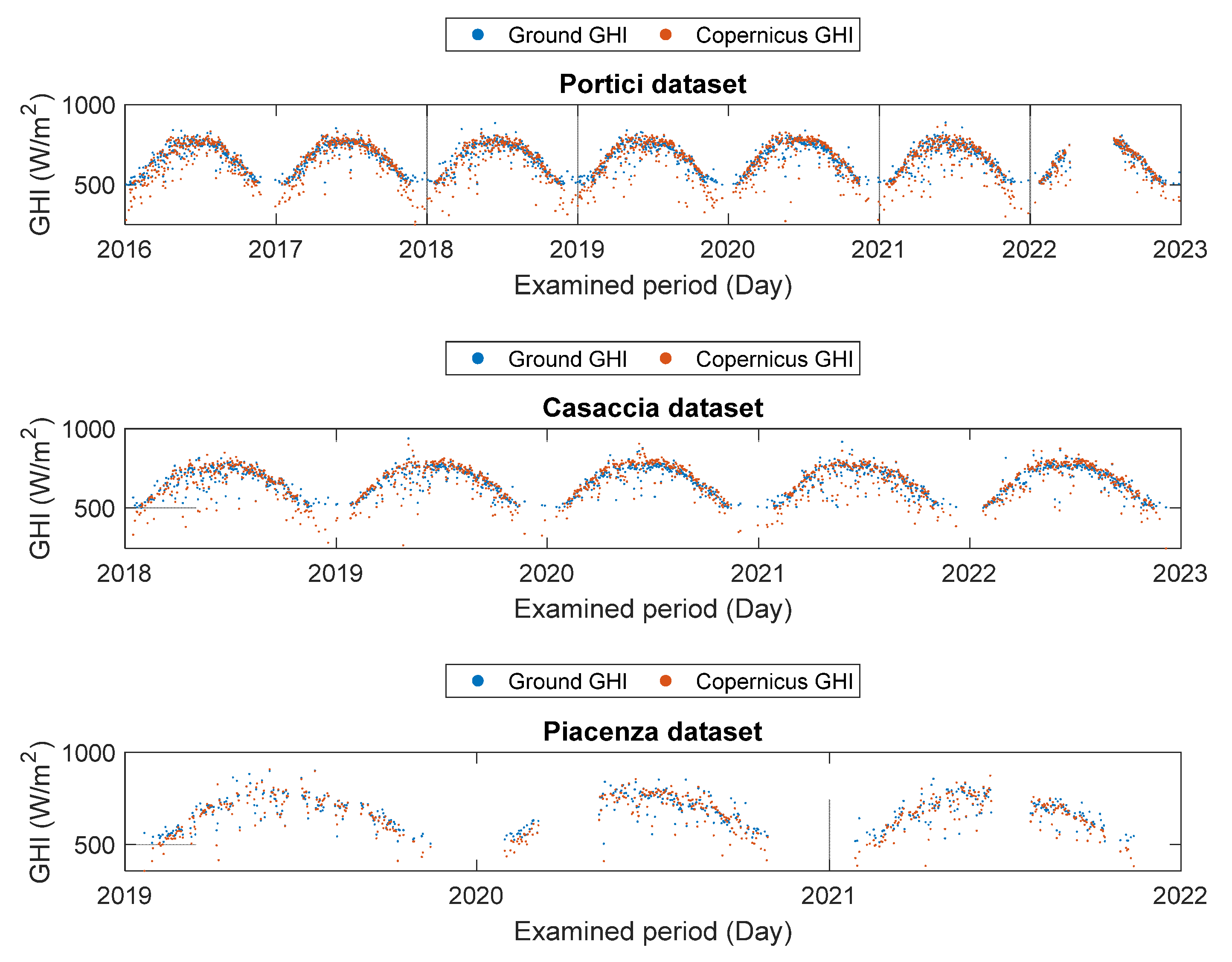
3.2. Comparative Analysis of Daily Averaged Data

Similar analyses were performed of the daily averaged dataset. In Figure 2, daily averaged GHI behaviors are shown.

Figure A4, Figure A5 and Figure A6 in Appendix A show the scatterplot of GHI_cop vs. GHI_ground on a seasonal basis for the three daily averaged datasets.

In

Table 6. Mean relative error and R² metrics computed for seasonal GHI_cop and GHI_ground for the three daily averaged datasets.

	Season	Num. Samples	MRE	R2
Portici dataset	Spring	520	3.87%	0.74
	Summer	603	3.39%	0.70
	Autumn	370	7.50%	0.48
	Winter	353	8.37%	0.43
Casaccia dataset	Spring	412	3.97%	0.73
	Summer	451	3.31%	0.76
	Autumn	222	7.18%	0.42
	Winter	202	5.82%	0.48
Piacenza dataset	Spring	176	4.07%	0.61
	Summer	186	3.44%	0.73
	Autumn	71	7.11%	0.40
	Winter	87	6.90%	0.49

, the mean relative error and R² metrics, computed on seasonal basis, are reported for the three daily averaged datasets.

Similarly to the hourly averaged dataset, daily averaged threshold values were computed for each season and are reported in

Table 7. Threshold values for the absolute error evaluation. The reported values were computed for each season for the three daily averaged datasets.

Thresold Values per Season (W/m2)
Site	Spring	Summer	Autumn	Winter
Portici	61.32	48.27	99.70	103.49
Casaccia	60.88	37.32	94.62	86.24
Piacenza	77.87	50.88	83.69	72.24

. Finally, in

Table 8. Number of occurrences in which the absolute error values exceed the threshold values with respect to the total number of events, for each season and for the three daily averaged datasets.

Number of Events Where the Daily Absolute Errors Exceed the Computed Threshold Value per Season
Site	Spring	Summer	Autumn	Winter
Portici	50/520 = 10%	55/603 = 9%	50/370 = 13%	58/353 = 16%
Casaccia	40/412 = 10%	74/451 = 16%	24/222 = 11%	25/202 = 12%
Piacenza	14/176 = 8%	18/186 = 10%	12/71 = 17%	10/87 = 11%

, we show the seasonal occurrences of absolute errors exceeding the computed thresholds.

4. Discussion

The data in Table 3 show that, in all three cases, MRE values vary from 4% to 7%, with the highest MRE values occurring during autumn and winter. Correspondingly, for daily averaged data (Table 6), MRE values range from 4% to 8%, and even in this case higher MRE values occur during autumn and winter. In order to identify the factors affecting this seasonally different behavior, it may be more useful to evaluate the Mean Bias Error, which is less sensitive to possible outliers than the MRE. Analyzing MBE (

Table A2. Performance metrics computed for seasonal GHI_cop and GHI_ground for the three hourly averaged datasets. (MBE, MAE, and RMSE are expressed in W/m²).

	Season	Num Samples	MBE	MAE	RMSE	R
Portici dataset	Spring	3717	−6.01	31.18	49.84	0.94
	Summer	4761	6.20	27.39	42.49	0.95
	Autumn	1438	−12.38	33.52	54.15	0.82
	Winter	1320	−19.16	36.78	57.85	0.82
Casaccia dataset	Spring	2783	6.32	35.72	55.69	0.93
	Summer	3444	12.34	31.10	45.95	0.95
	Autumn	801	−9.26	35.14	54.11	0.79
	Winter	790	−5.86	28.17	47.93	0.83
Piacenza dataset	Spring	1101	−4.71	35.54	56.84	0.92
	Summer	1269	2.86	28.37	44.15	0.94
	Autumn	274	−33.10	41.53	63.23	0.75
	Winter	344	−32.78	37.01	52.04	0.86

and

Table A3. Performance metrics computed for seasonal GHI_cop and GHI_ground for the three daily averaged datasets.

	Season	Num Samples	MBE	MAE	RMSE	R
Portici dataset	Spring	520	−13.00	27.08	40.88	0.88
	Summer	603	2.40	24.05	34.06	0.83
	Autumn	370	−28.49	42.23	65.28	0.75
	Winter	353	−36.42	47.60	70.25	0.72
Casaccia dataset	Spring	412	0.14	27.62	41.07	0.86
	Summer	451	8.98	23.44	29.95	0.89
	Autumn	222	−22.92	40.56	62.23	0.68
	Winter	202	−19.89	33.44	54.48	0.72
Piacenza dataset	Spring	176	−9.16	28.98	48.45	0.79
	Summer	186	−1.62	23.84	34.82	0.85
	Autumn	71	−39.87	42.22	59.23	0.74
	Winter	87	−38.05	39.48	53.37	0.82

, Appendix A), GHI_cop always underestimates GHI_ground in autumn and winter, for all three examined sites.

There are several possible reasons why the satellite solar irradiance data obtained from the Copernicus system overestimate ground-based measurements:

• Spatial resolution: Copernicus satellite data may show a coarser spatial resolution compared to ground-based measurements from monitoring stations. This can result in the averaging of solar radiation values over larger areas, leading to an overestimation compared to point measurements on the ground.
• Calibration errors: calibration errors can occur in both satellite data and ground-based measurements. However, if the satellite data are not properly calibrated or if there are discrepancies in calibration compared to the ground-based sensors, it can lead to an overestimation of solar radiation values.
• Atmospheric effects: satellite data can be affected by atmospheric effects such as the absorption or scattering of solar radiation during its passage through the atmosphere. These atmospheric effects may not be adequately accounted for by the satellite data and they could result in an overestimation of solar radiation values compared to ground-based measurements.
• Soiling effects on the ground instrumentation surface [33].
• Effect of different viewing geometries such as sun-glint or parallax effects.

The issues reported above may, however, exhibit different effects on daily and hourly timeframes. For instance, the effect of the different viewing geometries becomes particularly relevant when examining the hourly data [34,35,36,37]. The satellite’s spatial averaging throughout the day may lead to a reduction in precision during specific hours. On the other hand, daily data accumulate this spatial overestimation, impacting the overall daily total. A similar effect on daily and hourly overestimations can result from calibration errors. Throughout the day, variations in atmospheric conditions can lead to discrepancies in the calibration of hourly data. Meanwhile, if calibration errors persist over the entire day, their cumulative effect becomes more pronounced in the daily data. The influence of atmospheric effects is somewhat similar. Hourly data, being more sensitive to changing weather conditions, can exhibit fluctuations in solar radiation values due to atmospheric phenomena. In contrast, daily data reflect the cumulative impact of these atmospheric effects over the course of the day. Finally, considering the soiling effect on ground instrumentation surfaces, the variations in soiling throughout the day can have a distinct impact on the hourly data, depending on factors like weather conditions. Daily data, however, capture the overall influence of soiling during the entire 24 h period. In summary, the distinction between hourly and daily data lies in their sensitivity to temporal changes. Hourly data provide insights into the dynamic fluctuations occurring throughout the day, while daily data encapsulate the comprehensive impact over a full 24 h cycle. Each temporal scale contributes to the overall understanding of how the Copernicus system’s solar irradiance data may exhibit overestimation when compared to precise ground-based measurements.

As we have shown, in some cases, Copernicus satellite irradiance data may also underestimate ground-based measurements. This can occur in the following scenarios:

• Atmospheric conditions: Satellite measurements are affected by atmospheric conditions such as cloud cover, aerosols, and atmospheric scattering. These factors can affect the accuracy of satellite-derived solar radiation data, potentially resulting in an underestimation compared to ground-based measurements that are not affected by the same atmospheric conditions.
• Instrument calibration: Errors in instrument calibration can occur in both satellite sensors and ground-based measurement instruments. If the satellite sensors are not properly calibrated, or if there are discrepancies in calibration compared to the ground-based instruments, this can lead to an underestimation of solar radiation values in the satellite data.
• Surface reflectance: Satellite measurements rely on the reflection of solar radiation from the Earth’s surface. Short-term variations in surface reflectance properties, such as differences in surface materials or vegetation cover, can affect the accuracy of satellite-derived solar radiation data and result in underestimation compared to ground-based measurements.

The assessment of potential underestimation in Copernicus satellite irradiance data with respect to ground-based measurements requires careful consideration of some factors, particularly when examining both hourly and daily datasets.

Concerning atmospheric conditions, the hourly analysis denotes the presence of fluctuations in underestimation that can be related to variations in atmospheric elements throughout the day. On a daily scale, the cumulative effect of these atmospheric conditions over the 24 h period manifests as a general underestimation trend. Regarding the instrument calibration, the hourly examination highlights the impact of calibration errors on underestimation, as these errors introduce variations influenced by dynamic atmospheric conditions and instrument performance changes throughout the day. For daily data, a more comprehensive perspective emerges. Persistent calibration issues uniformly contribute to the total daily underestimation, with each hourly interval playing a role in shaping the aggregate result. Surface reflectance introduces fluctuations in the underestimations of the hourly averaged data as a result of changes in the surface properties during specific hours. In the daily context, the cumulative influence of surface reflectance variations over the course of the day contributes to a comprehensive daily underestimation. In summary, the analysis of underestimation in Copernicus satellite irradiance data involves distinct contributions from each factor [38] when considering hourly and daily datasets.

The above analysis shows that underestimates or overestimates are, therefore, possible for a variety of reasons during the whole course of a year, without showing any particular specificity that could be correlated to a seasonal trend, as is instead shown at both hourly and daily levels in Table 3 and Table 6, respectively. It is, therefore, quite natural to assume that those trends could be correlated with other factors, such as the height of the sun, which varies over the course of the year in exactly the same way as the observed hourly and daily variabilities. In other words, it is possible to hypothesize that more errors are recorded in the seasons in which the sun is lower on the horizon, even if this hypothesis requires further investigation.

5. Conclusions

The analysis was performed on three ground reference solar irradiance measurement stations, located at different Italian sites, comparing both their hourly and daily measurements with Copernicus-system-derived solar irradiance values, mainly to evaluate their relative differences in terms of MRE.

The comparative analysis has shown that, at least in the solar radiation limits as defined by the IEC 61724-2 Standard [12], a maximum MRE of <7% for hourly averaged GHI and a maximum MRE of <9% for daily averaged GHI are reported, confirming that Copernicus data for solar irradiance are reliable enough to be used at the hourly and daily levels, at least with the uncertainties reported here.

Interestingly enough, MRE values at hourly and daily levels exhibited a clear seasonal dependence, such that lower MRE values (and higher R² values) are observed to occur during spring and summer for both hourly and daily averaged data. Specifically, in spring and summer, the MRE ranges from 3.97% to 5.04% for the three hourly datasets and R² ranges from 0.84 to 0.91. In daily datasets, performances are even better, as we obtained an MRE ranging from 3.31% to 4.07% and an R² ranging from 0.61 to 0.76. Correspondingly, in autumn and winter, we obtained an MRE varying from 4.75% to 6.85% and R² values ranging from 0.46 to 0.69 for hourly datasets. For daily datasets, MRE ranges from 5.82% to 8.37% and R² ranges from 0.40 and 0.49.

To identify the possible conditions affecting these seasonally different performances, we evaluated the mean bias error. Analyzing the bias error, it could be observed that, in autumn and winter, GHI_cop always underestimates GHI_ground, in both hourly and daily datasets. As a matter of fact, several conditions exist, as listed in the Discussion paragraph, that could result in such a behavior, although none of them seems to be more likely to occur on a seasonal basis. The different atmospheric and environmental conditions typical of these seasons may affect these results. During spring and summer, for example, the reduced presence of clouds could reduce the absorption and scattering of solar radiation, improving the accuracy of satellite estimates and contributing to lower MREs. During autumn and winter, the increased presence of rains could increase the difficulties in accurately measuring solar radiation, contributing to worse performance indicators. Such conditions are, however, poorly correlated with seasonal variance, as discussed above. We therefore suggest that the observed effect can be more substantially correlated with the elevation of the sun, resulting in less noisy measurements being obtained for higher elevation angles. In any case, the obtained results suggest the feasibility of using Copernicus GHI as an alternative to ground data, as well as its use as an alternative to hourly and daily averaged data.

References

1. Copernicus. Available online: https://www.copernicus.eu/en (accessed on 8 January 2024).
2. Atmosphere Monitoring Service. Available online: https://atmosphere.copernicus.eu/ (accessed on 5 January 2024).
3. EQA Reports of Global Services. Available online: https://atmosphere.copernicus.eu/eqa-reports-global-services (accessed on 18 December 2023).
4. Rusen, S.E.; Aycan, K. Quality control of diffuse solar radiation component with satellite-based estimation methods. Renew. Energy 2020, 145, 1772–1779. [Google Scholar]
5. Polo, J.; Wilbert, S.; Ruiz-Arias, J.A.; Meyer, R.; Gueymard, C.; Šúri, M.; Pomares, L.M.; Mieslinger, T.; Blanc, P.; Grant, I.; et al. Integration of Ground Measurements with Model-Derived Data; A Report of IEA SHC Task 46 Solar Resource Assessment and Forecasting, Solar Heating and Cooling Programme, International Energy Agency, (October), 2015; pp. 1–34.
6. Verbois, H.; Saint-Drenan, Y.-M.; Becquet, V.; Gschwind, B.; Blanc, P. Retrieval of surface solar irradiance from satellite using machine learning: Pitfalls and perspectives, EGUsphere 2023, preprint. [CrossRef]
7. Fernández-Peruchena, C.M.; Polo, J.; Martín, L.; Mazorra, L. Site-Adaptation of Modeled Solar Radiation Data: The SiteAdapt Procedure. Remote Sens. 2020, 12, 2127. [Google Scholar] [CrossRef]
8. Romano, F.; Cimini, D.; Cersosimo, A.; Di Paola, F.; Gallucci, D.; Gentile, S.; Geraldi, E.; Larosa, S.; Nilo, S.T.; Ricciardelli, E.; et al. Improvement in Surface Solar Irradiance Estimation Using HRV/MSG Data. Remote Sens. 2018, 10, 1288. [Google Scholar] [CrossRef]
9. Hakuba, M.Z.; Folini, D.; Sanchez-Lorenzo, A.; Wild, M. Spatial representativeness of ground-based solar radiation measurements. J. Geophys. Res. Atmos. 2013, 118, 8585–8597. [Google Scholar]
10. Tong, L.; He, T.; Ma, Y.; Zhang, X. Evaluation and intercomparison of multiple satellite-derived and reanalysis downward shortwave radiation products in China. Int. J. Digit. Earth 2023, 16, 1853–1884. [Google Scholar]
11. IEC Webstore: Photovoltaic System Performance—Part 1: Monitoring. Available online: https://webstore.iec.ch/publication/65561 (accessed on 9 December 2021).
12. IEC Webstore: Photovoltaic System Performance—Part 2: Capacity Evaluation Method. Available online: https://webstore.iec.ch/publication/25982 (accessed on 16 October 2021).
13. Vuilleumier, L.; Meyer, A.; Stöckli, R.; Wilbert, S.; Zarzalejo, L.F. Accuracy of satellite-derived solar direct irradiance in Southern Spain and Switzerland. Int. J. Remote Sens. 2020, 41, 8808–8838. [Google Scholar]
14. CAMS Radiation Service. Available online: https://www.soda-pro.com/web-services/radiation/cams-radiation-service (accessed on 14 January 2024).
15. Yang, D.; Bright, J.M. Worldwide validation of 8 satellite-derived and reanalysis solar radiation products: A preliminary evaluation and overall metrics for hourly data over 27 years. Sol. Energy 2020, 210, 3–19. [Google Scholar]
16. Salazar, G.; Gueymard, C.; Galdino, J.B.; de Castro Vilela, O.; Fraidenraich, N. Solar irradiance time series derived from high-quality measurements, satellite-based models, and reanalyses at a near-equatorial site in Brazil. Renew. Sustain. Energy Rev. 2020, 117, 109478. [Google Scholar]
17. Jiang, H.; Lu, N.; Qin, J.; Tang, W.; Yao, L. A deep learning algorithm to estimate hourly global solar radiation from geostationary satellite data. Renew. Sustain. Energy Rev. 2019, 114, 109327. [Google Scholar]
18. Linares-Rodriguez, A.; Ruiz-Arias, J.A.; Pozo-Vazquez, D.; Tovar-Pescador, J. An artificial neural network ensemble model for estimating global solar radiation from Meteosat satellite images. Energy 2013, 61, 636–645. [Google Scholar]
19. Kaba, K.; Sarıgül, M.; Avcı, M.; Kandırmaz, H.M. Estimation of daily global solar radiation using deep learning model. Energy 2018, 162, 126–135. [Google Scholar]
20. Janjai, S.; Pankaew, P.; Laksanaboonsong, J.; Kitichantaropas, P. Estimation of solar radiation over Cambodia from long-term satellite data. Renew. Energy 2011, 36, 1214–1220. [Google Scholar]
21. Ayaz, A.; Irfan, M.A.A.; Noman, M. Comparison of Satellite and Ground based Solar Data for Peshawar Pakistan. Int. J. Eng. Work. 2019, 6, 288–291. [Google Scholar]
22. Ayaz, A.; Ahmad, F.; Irfan, M.A.A.; Rehman, Z.; Rajski, K.; Danielewicz, J. Comparison of Ground-Based Global Horizontal Irradiance and Direct Normal Irradiance with Satellite-Based SUNY Model. Energies 2022, 15, 2528. [Google Scholar]
23. Olomiyesan, B.M.; Oyedum, O.D. Comparative study of ground measured, satellite-derived, and estimated global solar radiation data in Nigeria. J. Sol. Energy 2016, 2016, 1–7. [Google Scholar]
24. Camargo, L.R.; Dorner, W. Comparison of satellite imagery-based data, reanalysis data and statistical methods for mapping global solar radiation in the Lerma Valley (Salta, Argentina). Renew. Energy 2016, 99, 57–68. [Google Scholar] [CrossRef]
25. Federico, S.; Torcasio, R.C.; Sanò, P.; Casella, D.; Campanelli, M.; Meirink, J.F.; Wang, P.; Vergari, S.; Diémoz, H.; Dietrich, S. Comparison of hourly surface downwelling solar radiation estimated from MSG–SEVIRI and forecast by the RAMS model with pyranometers over Italy. Atmos. Meas. Tech. 2017, 10, 2337–2352. [Google Scholar] [CrossRef]
26. Psiloglou, B.E.; Kambezidis, H.D.; Kaskaoutis, D.G.; Karagiannis, D.; Polo, J.M. Comparison between MRM simulations, CAMS and PVGIS databases with measured solar radiation components at the Methoni station, Greece. Renew. Energy 2020, 146, 1372–1391. [Google Scholar]
27. Antonanzas-Torres, F.; Cañizares, F.; Perpiñán, O. Comparative assessment of global irradiation from a satellite estimate model (CM SAF) and on-ground measurements (SIAR): A Spanish case study. Renew. Sustain. Energy Rev. 2013, 21, 248–261. [Google Scholar]
28. CMSAF. Available online: https://www.cmsaf.eu/EN/Home/home_node.html (accessed on 12 December 2023).
29. Huang, G.; Li, Z.; Li, X.; Liang, S.; Yang, K.; Wang, D.; Zhang, Y. Estimating surface solar irradiance from satellites: Past, present, and future perspectives. Remote Sens. Environ. 2019, 233, 111371. [Google Scholar]
30. ISO 9060:2018; Solar Energy—Specification and Classification of Instruments for Measuring Hemispherical Solar and Direct Solar Radiation. International Organization for Standardization: Geneva, Switzerland, 2018. Available online: https://standards.iteh.ai/catalog/standards/sist/1ec73ab8-4e64-4e2e-91e4-7f9a0a2f3b43/iso-9060-2018 (accessed on 18 March 2024).
31. ISO 8601; Date and Time Format. International Organization for Standardization: Geneva, Switzerland, 2022. Available online: https://www.iso.org/iso-8601-date-and-time-format.html (accessed on 18 March 2024).
32. SOLPOS Calculator. Available online: https://midcdmz.nrel.gov/solpos/solpos.html (accessed on 4 October 2023).
33. Esposito, E.; Leanza, G.; Di Francia, G. Soiling Detection Investigation in Solar Irradiance Sensors Systems. In Sensors and Microsystems; Di Francia, G., Di Natale, C., Eds.; AISEM 2022; Lecture Notes in Electrical Engineering; Springer: Cham, Switzerland, 2023; Volume 999. [Google Scholar]
34. Lu, X. Estimation of the Instantaneous Downward Surface Shortwave Radiation Using MODIS Data in Lhasa for All-Sky Conditions (2016); International Development, Community and Environment (IDCE): Worcester, MA, USA, 2016; Available online: https://commons.clarku.edu/idce_masters_papers/99 (accessed on 17 December 2023).
35. Wang, T.; Shi, J.; Husi, L.; Zhao, T.; Ji, D.; Xiong, C.; Gao, B. Effect of Solar-Cloud-Satellite Geometry on Land Surface Shortwave Radiation Derived from Remotely Sensed Data. Remote Sens. 2017, 9, 690. [Google Scholar]
36. Müller, R.; Pfeifroth, U. Remote sensing of solar surface radiation—A reflection of concepts, applications and input data based on experience with the effective cloud albedo. Atmos. Meas. Tech. 2022, 15, 1537–1561. [Google Scholar] [CrossRef]
37. User Guide to the CAMS Radiation Service (CRS). 2021. Available online: https://atmosphere.copernicus.eu/sites/default/files/2022-01/CAMS2_73_2021SC1_D3.2.1_2021_UserGuide_v1.pdf (accessed on 17 December 2023).
38. User’s Guide to the CAMS Radiation Service (CRS). 2018. Available online: https://atmosphere.copernicus.eu/sites/default/files/2019-01/CAMS72_2015SC3_D72.1.3.1_2018_UserGuide_v1_201812.pdf (accessed on 24 September 2019).
39. National Solar Radiation Database. Available online: https://nsrdb.nrel.gov/ (accessed on 15 December 2023).
40. CERES Project. Available online: https://ceres.larc.nasa.gov/ (accessed on 31 December 2023).
41. SOLCAST. Available online: https://solcast.com/ (accessed on 27 December 2023).
42. INPE. Available online: https://satelite.cptec.inpe.br/radiacao/ (accessed on 27 December 2023).
43. Meteonorm. Available online: https://meteonorm.com/ (accessed on 17 January 2024).
44. NASA—The POWER Project. Available online: https://power.larc.nasa.gov/ (accessed on 12 January 2024).
45. SWERA. Available online: https://s3.amazonaws.com/openei-public/swera.zip (accessed on 31 October 2022).
46. ECMWF. Available online: https://www.ecmwf.int (accessed on 16 March 2024).
47. LSASAF. Available online: https://landsaf.ipma.pt/en/ (accessed on 14 March 2024).
Figure 1. Hourly averaged GHI behavior during the examined period for the three analyzed datasets. Red dots represent Copernicus GHI; blue dots represent Ground GHI. It is worth noting that some periods of missing data exist in each dataset.
Energies 17 01579 g001
Figure 2. Daily averaged GHI behavior during the examined period for the three analyzed datasets. Red points represent Copernicus GHI; blue points represent Ground GHI.
Energies 17 01579 g002