Article

Attractive Ellipsoid Technique for a Decentralized Passivity-Based Voltage Tracker for Islanded DC Microgrids

by
Alexander S. Poznyak
1,
Hisham M. Soliman
2,
Hussain Alazki
3,
Ehab H. E. Bayoumi
4 and
Michele De Santis
5,*
1
Departamento de Control Automatico, A.P. 14-740, CINVESTAV, Mexico D.F. 07000, Mexico
2
Department of Electrical Power Engineering, Faculty of Engineering, Cairo University, Cairo 12613, Egypt
3
Faculty of Engineering, Autonomous University Carmen, Cd. del Carmen 24180, Mexico
4
Department of Mechanical Engineering, Faculty of Engineering, The British University in Egypt, El Sherouk City 11837, Egypt
5
Department of Engineering, University of Campania “Luigi Vanvitelli”, 81031 Aversa, Italy
*
Author to whom correspondence should be addressed.
Energies 2024, 17(7), 1529; https://doi.org/10.3390/en17071529
Submission received: 15 January 2024 / Revised: 22 February 2024 / Accepted: 19 March 2024 / Published: 22 March 2024
(This article belongs to the Section A1: Smart Grids and Microgrids)

Abstract

:
A new passivity-based voltage tracker for islanded Direct Current (DC) microgrids is presented in this paper. The proposed design develops a new sufficient condition for passivity-based state feedback with proportional and integral control using the attracting ellipsoid method. In this paper, we consider the time behavior of the extended vector, which completely describes the principle properties of the closed-loop system such as the boundedness of the trajectories within some ellipsoid and the dependence of its “size” on the feedback gains. The next step, which we are realizing in this paper, is the minimization of the attractive ellipsoid by selecting the “best” admissible feedback parameters. Here, it is important to note that the applied feedback is of PD-type (proportional differential) on the system state and I-type (integral) on the output. This is a new construction of the suggested feedback which gives several advantages for a designer. The suggested control is decentralized and uses only the local states; it is cost-effective and avoids the time delays in the communication networks which are needed if centralized control is used. The suggested control is carried out in the bilinear matrix inequality (BMI) framework. Extensive simulation is performed on a test system composed of renewable energy sources, under plug and play (PnP) operations, and uncertainties in distribution lines and loads. The performance of the proposed decentralized voltage controller is compared with that of a voltage tracker present in the literature. The comparison shows the improvements introduced by the proposed control ensure the stability of the dc bus voltage and a quick response under different scenarios of operating conditions.

1. Introduction

Electricity has evolved into more than just a source of energy; it has become an integral part of our daily life. However, a large amount of people do not have access to electricity in today’s world. Being so far from the main electrical grid system or the high cost of connecting the grid line to rural places are the main barriers to providing such such large amounts of people with electricity. As a result, the solution to this challenge is to combine conventional and nonconventional electricity generation (renewable sources).
The widespread adoption of renewable energy sources (solar and wind) and other alternative types of energy supply have led to a high level of distributed generation (DG) in power networks [1,2]. DG has an impact on the electrical network, causing voltage changes and power imbalances [3], posing additional control challenges. The electrical network is separated into smaller sections known as microgrids (MGs) in order to study these concerns. An MG is an interconnection of generators, loads, and storage systems, with defined electrical boundaries, that can work together as a single controllable unit, in an isolated or utility grid-connected manner, to reliably supply power [1,2,3,4].
DC microgrids (DC-MG) are a promising way to combine electric vehicles, batteries, and solar power [1,2,3,5]. When compared to more traditional AC microgrids, they offer inherent advantages in terms of efficiency and controllability. Conversely to AC electrical networks, a DC-MG does not require reactive power or frequency regulation [6]. It also requires fewer stages of conversion and fewer wires, lowering the grid’s overall cost. In a DC-MG, loads, storage devices, and renewable energy sources are all connected to a DC bus.
There are three types of control hierarchies in general: primary, secondary, and tertiary. The primary control stabilizes the system’s operation, while the secondary control guarantees that the system meets the reference voltage, and the droop or non-droop control approach is used [5]. The economic and/or environmental aspects are considered by the tertiary control [7]. Local information is typically used in primary control, whereas communication between converters is used in secondary and tertiary control.
There are many control schemes for each level in a hierarchical control strategy. For primary control, the DC bus signaling [8], droop control [9], and fuzzy control [10,11] are commonly used. Distributed, decentralized, and centralized control are used for secondary control. For tertiary control, the genetic algorithm (GA) [12], particle swarm algorithm [13], consensus algorithm, etc., are utilized [14,15,16,17,18,19]. Each of these control methods has its own set of advantages and disadvantages. Thus, it is difficult for any control designer to pick one without risking the system’s ultimate aims.
Based on the type of controller, and communication link, MG control systems may be categorized into three categories: (i) centralized control systems, (ii) decentralized control systems, and (iii) distributed control systems.
(i)
Centralized control.
In centralized control, communication lines connect each MG to a central controller. The central controller collects information from converters located at various locations, uses it to make the control signal, and then send commands to the converters. It provides impressive control in MGs. The requirement for massive communication networks, as well as a single-point failure, are the key disadvantages of centralized control.
(ii)
Decentralized control.
The distributed generators are controlled by autonomous local controllers via independent local variables in a decentralized controller and there is no communication medium in the control. Despite its limitations owing to the lack of a communication link, this control approach is regarded as the most reliable. In addition, decentralized control has the plug and play capability [20]. The Droop Control [21] is a widely established decentralized control method that provides essentially fair voltage and current regulation. A passivity-based control is proposed in [22] for the voltage stabilization of a DC-MG. It considers the dynamic RLC lines and nonlinear loads.
(iii)
Distributed control.
This control approach combines the benefits of a centralized and a decentralized controller. The controller of each distributed generator communicates with its neighbors via a communication medium with limited bandwidth. The implementation of a centralized control strategy becomes more difficult as the number of DG units grows. The distributed controller proves to be a stronger competitor in such a situation. A further benefit of such a controller is that it keeps the system running even if the communication link fails, making it resilient to a single-point failure. The main shortcomings are bus voltage variation, complex analytic behavior, and power tracking errors.

1.1. Paper Contribution

The MG dynamics is nonlinear. Thus, the passivity-based control is utilized as it is an effective method for nonlinear systems. The reader is referred to [23,24] for details on passivity-based control.
If the designer requires a faster response than given by the state feedback with integral control [5,25,26], by the ellipsoidal approach, a proportional element is added. The resulting state feedback with PI control could not be designed by the ellipsoidal approach in [5,26]; however, the present passivity-based method succeeds in this regard.
Although there has been a lot of research efforts into applying passivity control to electric machines and power converters, there has been little research into DC-MGs [27,28,29,30,31].
In comparison to prior approaches, this study presents a decentralized passivity-based control for the primary control of DC-MGs, which has the following advantages:
  • A new design is developed for a decentralized state feedback with PI control.
  • Decentralized control is achieved by breaking down the DC global MG system into subsystems. The impact of other subsystems on a single subsystem is considered a disturbance that should be rejected. This is achieved by minimizing the size of the attracting ellipsoid.
  • A new sufficient stability condition is derived in terms of bilinear matrix inequality.
  • Different testing plug and play operations, line parameter uncertainties, and load variations show the effectiveness of the proposed design.
To the best of authors’ knowledge, the proposed passivity design of the decentralized PI is developed for the first time.
Section 2 presents modeling of the test DC-MG and problem formulation; the problem’s solution is given in Section 3 and Section 4. Section 5 deals with the simulation’s validation. Section 6 contains the conclusions. Finally, an appendix is given in the last section, Appendix A.

1.2. Notations and Facts

The notation X 0 ( X > 0 ) indicates that the real symmetric matrix X is positive semi-definite (respectively, positive definite) throughout this work. I is the identity matrix, with the appropriate dimension. The transposition of the matrix N is denoted by the symbol N T . If not specifically specified, it is presumed that matrices have compatible dimensions. The notation ( . ) is the Euclidean matrix norm of (.). In symmetric block matrices, a term that is induced by symmetry is denoted by an asterisk (∗).
Fact 1: 
This fact can be used to eliminate the time-varying uncertainty Δ (t)
M Δ t N + < ϵ M M T + ϵ 1 N T N
Fact 2 (Schur complements) : 
Given a matrix M composed of:
M = M 1 M 3 M 2
where M 1 = M 1 T , M 2 = M 2 T > 0 , then M > 0 if and only if
M 1 M 3 M 2 1 M 3 T > 0 .
Fact 2 is used to convert the last nonlinear matrix equation to a linear one.

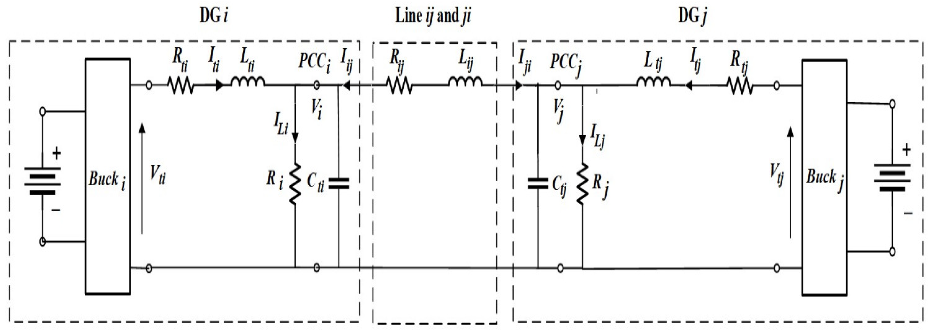
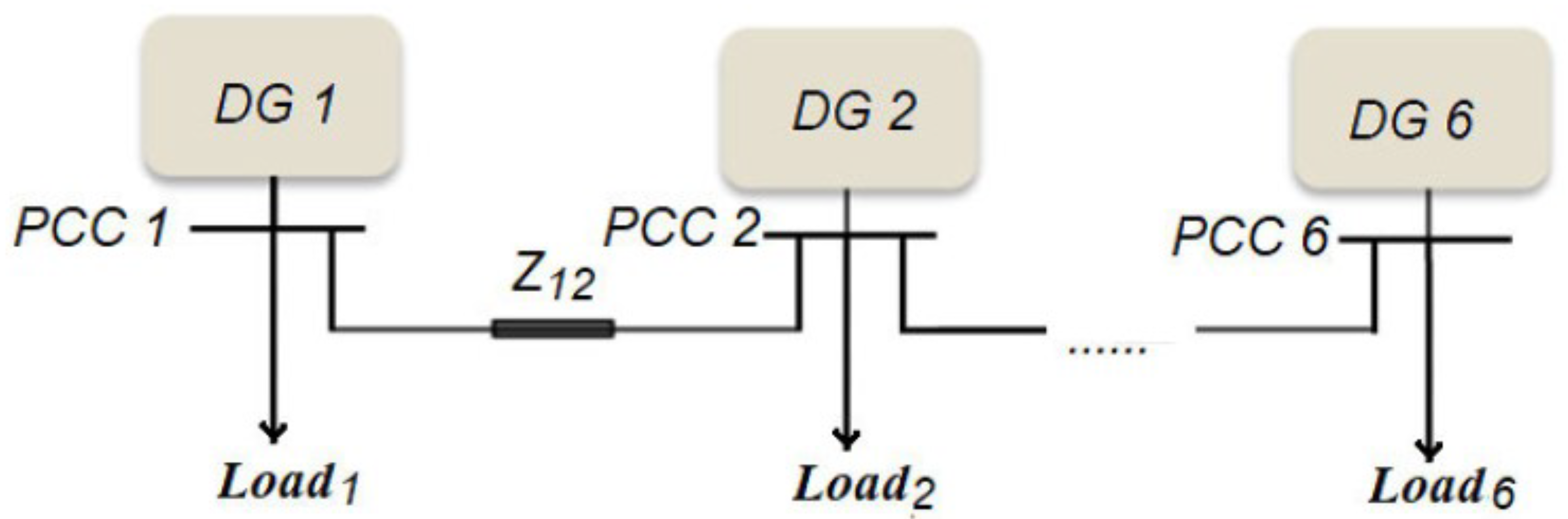
2. System Modeling and Problem Formulation

The concept of two parallel DGs is extended to MGs with N DGs. As shown in Figure 1, the linkages between two DGs i and j are represented by a DC line with an impedance of R i j and L i j [20,32].
The DC voltage sources in Figure 1 can be considered photovoltaic (PV) sources; each DG has its dc-dc converter. PV voltage sources will fluctuate since solar radiation is irregular in nature. For the sake of this study, it is expected that the PV generator incorporates a storage mechanism in order to maintain a constant output voltage.
The following state space equations for DG # i can be used to describe the islanded DC-MG for N DGs in Figure 1:
d V i d t = 1 C t i I t i 1 C t i I L i + 1 C t i I i j
d I t i d t = 1 L t i V i R t i L t i I t i + 1 L t i V t i
Line i j : d I i j d t = R i j L i j I i j + 1 L i j V j 1 L i j V i
Given that L i j is very small, d I i j d t = 0 , therefore:
I i j = V j V i R i j
d I t i d t = 1 L t i V i R t i L t i I t i + 1 L t i V t i
d V i d t = 1 C t i I t i 1 C t i I L i + 1 C t i R i j V j 1 C t i R i j V i
The following state space equations can be used to describe the islanded DC-MG with N DGs in Figure 1:
x ˙ i = ( A i i + Δ A i i ) x i + B i u i + D i x , y i = C i , z i = H i x i
where x i = V i I t i T , u i = V t i , y i = z i = V i are the vectors of states, input, output for feedback, and output to be optimized, respectively. Additionally, x = x 1 x N , with the matrices A i j , B i , H i
A i i = 1 C i j 1 R i j 1 R i C t i 1 C t i 1 L t i R t i L t i
Δ A i i = Δ R i R i 2 C t i 0 0 0 , A i j = 1 R i j C t i 0 0 0
The external disturbance is
D i = A i 1 O i i A i j A i N
j = 1 N , j i
B i = 0 1 L t i , C i = H i = 1 0
Since most distribution systems are radial, the DC-MG study system is selected with a radial structure, Figure 2. As shown in Figure 2, the study islanded DC-MG is made up of 6 DGs. However, the proposed control can be applied to any other number of DGs.
The system data are given in Table 1 and Table 2. Note that the above modeling is given in many references. We added small modifications.
The proposed control technique should satisfy the following requirements:
  • The closed-loop system asymptotically follows all reference voltage signals, providing the desired transient and steady-state performance in compliance with IEEE standards [33].
  • The controller ensures the overall MG system’s asymptotic stability.
  • In MGs, the PnP functionality of DGs is allowed.
  • The controller is resilient to changes in MG topology and load variations.
  • The voltage controller is decentralized, with a local controller for each DG and no communication link.
  • Decentralization provides several advantages in terms of reliability and cost-effectiveness.
Consider a linear time-invariant controllable system
x ˙ = A x + B u , y = C x
The output must follow the input in the control system architecture. The control problem is known as a regulator problem when the input is constant. A tracking problem occurs when the input is time-varying. In this section, a decentralized controller for the scheme in (16) is created. The composite scheme in (16) can be broken down into N-subsystems. In (16), decompose the matrix A = { A i j , i , j = 1 , . . N } into two parts: diagonal, A d , and off-diagonal, D.
x ˙ = A d x + B u + D w , y = C x
where
A d = A 11 0 0 0 . . 0 0 0 A N N , B = B 1 0 0 0 . . 0 0 0 B N , D = D 1 . . D N = 0 . . A 1 N . . . . . . A N 1 . . 0 and C = C 1 0 0 0 . . 0 0 0 C N
In (17), the impact of the remainder of the system on a particular subsystem is regarded as an external disturbance, D w , which the proposed controller has to reject. The external bounded disturbance w is considered to be the vector x.
There is no integrator in the MG model (16) (so it is a type 0 plant). As a result, given a step input, there is going to be a steady-state error. The output voltage must track the reference voltage with no errors. An integrator should be placed in the feedforward channel between the error comparator and the plant. To speed up the system response, a proportional part is added in parallel with an integral part.
For each DG unit, a decentralized dynamic voltage tracker with the following structure is required:
u = K x + K I ξ + K P e , ξ ˙ = r C x , e = r C x
where
K = K 1 0 0 0 . . 0 0 0 K N , K I = K 1 , I 0 0 0 . . 0 0 0 K N , I , K P = K 1 , P 0 0 0 . . 0 0 0 K N , P
Note that the structure of the proposed voltage tracker is a state feedback with P I .
Models:
x ˙ i = A i i x i + B i u i + D i w i R n y i = C i x i R m , i = 1 , . . . , N u i R k , w i R r n = 2 , m = 1 , k = 1 , r = 12 , N = 6
Extended system model:
x = x 1 , . . . , x N , w = w 1 , . . . , w N
x ˙ = A x + B u + D w R n × N y = C x R m × N , w R n × N u R k × N

3. Passivity-Based Control Using the Attracting Ellipsoid Method

3.1. Solution Methodology

In this paper:
  • we consider the time behavior of the extended vector x ¯ = x ˚ , e ˚ , x ˚ : = x x 0 , e ˚ : = e e 0 which completely describes the principle properties of the closed-loop system such as boundedness of the trajectories x ¯ within some ellipsoid and the dependence of its ”size” on the feedback gains;
  • the next step, which we are realizing, is the minimization of the attractive ellipsoid by selecting the “best” admissible feedback parameters.
Consider a linear stationary system given by the following equations
x ˙ t = A x x t + B w w t x 0 = x 0 is fixed z t = C z x x t + D z w w t
where x t R n is the state of the system at time t, z t R m is its output, and w t R k is an external input.

3.2. Dissipativity Property

Lemma 1. 
The extended version of η-dissipativity property.
If for the system (24) and some nonnegative matrix P 1 = P 1 > 0 the following Linear Matrix Inequality (LMI) takes place
P 1 A x + A x P 1 P 1 B w C z x B w P 1 C z x 2 η I n × n D z w + D z w 0
then for all t t 0 0 and all x 0 , the following property holds
η t = t 0 t w τ w τ d τ t = t 0 t w τ z τ d τ + 1 2 x t 0 P 1 x t 0 x t P 1 x t
Proof. 
See Appendix A. □
Remark 1. 
In the partial case when x t 0 = 0 , we obtain
η t = t 0 t w τ w τ d τ t = t 0 t w τ z τ d τ 1 2 x t P 1 x t t = t 0 t w τ z τ d τ
which for η = 0 leads to the passivity property
0 t = t 0 t w τ z τ d τ

4. Main Result

Given an LMI Model
x ˙ = A x + B u + D w 0 R n y = C x R m , w 0 R r
Conversion to zero initial conditions:
Introduce the new variable
x ˚ : = x x 0
Then, (29) can be represented as
d d t x ˚ = A x ˚ + A x 0 + B u + D w 0 R n
and select
u = u c o m p + u ˚ , u c o m p : = K c o m p x 0 , K c o m p = B + A
where B + : is the pseudo-inverse of B, which leads to
d d t x ˚ = A x ˚ + A B K c o m p x 0 + B u ˚ + D w 0 R n
If the pair A , B is controllable, then there exists K c o m p = B + A such that
I B B + A = 0
and we obtain the following dynamics
d d t x ˚ = A x ˚ + B u ˚ + D w 0 , x ˚ = 0
Introduce also a new vector e ˚
e ˚ : = e e 0 , e 0 = r 0 C x 0 , e ˚ 0 = 0
an auxiliary variable
ξ ˚ t : = τ = 0 t e ˚ τ d τ
control
u ˚ = K x ˚ + K p e ˚ + K i ξ ˚ R k
and assumptions (if necessary)
A 1 : w 0 1 , w 0 R d A 2 : r ˙ r ˙ + <
In this paper, the time behavior of the extended vector x ¯ = x ˚ , e ˚ was considered, which completely describes the principle properties of the closed-loop system such as the boundedness of the trajectories x ¯ within some ellipsoid and the dependence of its “size” on the feedback gains; the next step, which was realized, is the minimization of the attractive ellipsoid by selecting the “best” admissible feedback parameters.

4.1. Closed-Loop System

The original system after compensation with zero initial conditions is as follows:
d d t x ˚ = A x ˚ + B u ˚ + D w 0 , x ˚ = 0 u ˚ = K x ˚ + K p e ˚ + K i ξ ˚ R k e ˚ : = e r 0 C x 0 = y C x e r 0 C x 0 , e ˚ 0 = 0

Extended Vector x ¯

For the extended vector
x ¯ = x ˚ e ˚ 0 R n + m , x ¯ 0 = 0
we have
d d t x ¯ = A x ˚ + B K x ˚ + K p e ˚ + K i ξ ˚ + D w 0 r ˙ C d d t x ˚ = A x ˚ + B K x ˚ + K p e ˚ + K i ξ ˚ + D w 0 r ˙ C A x ˚ + B K x ˚ + K p e ˚ + K i ξ ˚ + D w 0 = A + B K B K p C A + B K C B K p x ¯ + B K i 0 n × m C B K i I m × m ξ ˚ r ˙ + D C D w 0 A + B K B K p C A + B K C B K p A x ¯ x ¯ + B K i D 0 n × m C B K i C D I m × m B w ξ ˚ w 0 r ˙ w
Thus, finally, we have
d d t x ¯ = A x ¯ x ¯ + B w w

4.2. Ellipsoidal Approach

Consider the ellipsoid,
E = x ¯ P x ¯ < 1 , P > 0 ,
with the center in the origin and a configuration matrix P. Then, the trajectory x ¯ ( t ) will be attracted to the ellipsoid, and will not leave it, by choosing a Lyapunov function V > 0, and will require V ˙ < 0 as follows.
V = x ¯ P x ¯ , P = P x 0 0 P e R n + m × n + m
V ˙ = 2 x ¯ P d d t x ¯ = 2 x ¯ P x 0 0 P e A + B K B K p C A + B K C B K p x ¯ + B K i 0 n × m C B K i I m × m ξ ˚ r ˙ + D C D w 0 = x ¯ P x A + B K + A + B K P x P x B K p P e C ( A + B K ) P e C ( A + B K ) + P x B K p P e C B K p P e C B K p W x ¯ x ¯ + x ¯ P x B K i P x D 0 n × m P e C B K i P e C D P e C x ¯ , w ξ ˚ w 0 r ˙ w
or
V ˙ = x ¯ W x ¯ x ¯ + x ¯ C x ¯ , w w = x ¯ W x ¯ x ¯ C x ¯ , w x ¯ w
Defining
z = C x ¯ , w C z x ¯ x ¯ + D z w w = C z x ¯ x ¯ + D z w w C z x ¯ = P x B K i P x D 0 n × m P e C B K i P e C D P e = P x B K i P e C B K i P x D P e C D 0 m × n P e
we may represent (47) as
V ˙ = x ¯ W x ¯ x ¯ w z D z w w
Adding and subtracting the terms α x ¯ P x x ¯ with α > 0 , we obtain
V ˙ = x ¯ W ¯ x ¯ x ¯ α V + w D z w + D z w 2 w w z
where
W ¯ x ¯ = P x A + B K + A + B K P x + α P x P x B K p P e C ( A + B K ) P e C ( A + B K ) + P x B K p P e C B K p P e C B K p + + α P e
Integration of (49) within the interval t 0 , t and the application of (27) gives
V x ¯ t V x ¯ t 0 = x ¯ W ¯ x ¯ x ¯ α V + w D z w + D z w 2 w w z x ¯ W ¯ x ¯ x ¯ α V + w D z w + D z w 2 η I n + 2 m × n + 2 m w
Taking t 0 = t Δ t , 0 Δ t 0 and dividing by Δ t , in view of (43), we derive
V ˙ x ¯ W ¯ x ¯ x ¯ α V + w D z w + D z w 2 η I d + 2 m × d + 2 m w
Represent the matrix D z w as
D z w = D z w 1 , 1 0 m × d 0 m × m 0 d × m D z w 2 , 2 0 d × m 0 m × m 0 m × d D z w 3 , 3
Then, calculate
D z w + D z w 2 η I d + 2 m × d + 2 m
and
w D z w + D z w 2 η I d + 2 m × d + 2 m w = ξ ˚ 1 2 D z w 1 , 1 + D z w 1 , 1 η I m × m ξ ˚ + w 0 1 2 D z w 2 , 2 + D z w 2 , 2 η I d × d w 0 + r ˙ 1 2 D z w 3 , 3 + D z w 3 , 3 η I m × m r ˙
Taking
D z w 1 , 1 = η I m × m , D z w 2 , 2 = 1 + ε η I d × d ,
D z w 3 , 3 = 1 + ε η I m × m , ε > 0
we obtain
w D z w + D z w 2 η I d + 2 m × d + 2 m w =
ε w 0 2 + r ˙ 2 ε 1 + r ˙ + 2
which under the condition
W ¯ x ¯ 0
permits us to represent (52) as
V ˙ x ¯ t α V x ¯ t + ε 1 + r ˙ + 2
and, hence,
lim sup t V x ¯ t α 1 ε 1 + r ˙ + 2
or, equivalently,
lim sup t x ¯ t α ε 1 + r ˙ + 2 P x ¯ t 1
Remark 2. 
In this statement, we deal with the corresponding linear model where the feedback control contains PI terms with respect to the current state and the feedback with the output error. This is a new consideration in the frame of the Attractive Ellipsoid method (AEM). To work with the effect of this new term we apply the passivity ideas. In particular, the term w T z in (49) should be negative to then apply the AEM. Our proposition finally leads to (51) and (59).
We can formulate the main result as follows:
If the Linear Stationary System (LSS)
x ˙ = A x + B u + D w 0 R n y = C x R m , w 0 R r I B B + A = 0
controlled by
u = u c o m p + u ˚ , u c o m p : = B + A x 0 u ˚ = K x ˚ + K p e ˚ + K i ξ ˚ R k R k e = r y = r C x R m e ˚ : = e r 0 C x 0 , ξ ˚ t = τ = 0 t e ˚ τ d τ
there exist the nonnegative matrices P x , P e , P 1 , and positive constants α , ε such that the following matrix inequalities hold
W ¯ x ¯ = P x A + B K + A + B K P x + α P x P x B K p P e C ( A + B K ) P e C ( A + B K ) + P x B K p P e C B K p P e C B K p + α P e 0
and
P 1 A x + A x P 1 P 1 B w C z x ¯ B w P 1 C z x ¯ ε I m × m 0 m × d 0 m × m 0 d × m ε I d × d 0 d × m 0 m × m 0 m × d ε I m × m 0
where
A x : = A + B K B K p C A + B K C B K p , B w = B K i D 0 n × m C B K i C D I m × m , C z x ¯ = P x B K i P x D 0 n × m P e C B K i P e C D P e = P x B K i P e C B K i P x D P e C D 0 m × n P e
and then, for the extended vector
x ¯ = x ˚ e ˚ R n + m
we may guarantee that
lim sup t x ¯ t α ε 1 + r ˙ + 2 P x ¯ t 1
Remark 3. 
Notice that the relations (66) and (67) with respect to the unknown matrices (P,A,K, K P , and scalars ϵ, α) are BMI.

4.3. Nonlinear Optimization Problem

Under the applied conditions, the attractive ellipsoid is defined by the matrix
P a t t r = α ε 1 + r ˙ + 2 P
The optimization procedure, described above, (using MATLAB packages TOMLAB/PENBMI), leads to:
α = 1.34 10 05 , ε = 0.8100
K = 0.4786 0.3961 0 0 0 0 0 0 0.3789 0.1585 0 0 0 0 0 0 0.1384 0.4751 0 0 0 0 0 0 0 0 0 0 0 0 0 0 0 0 0 0 0 0 0 0 0 0 0 0 0 0 0 0 0 0 0 0 0 0 0.2449 0.3496 0 0 0 0 0 0 0.4204 0.3983 0 0 0 0 0 0 0.4255 0.3749
K p = 1.4355 0 0 0 0 0 0 1.6407 0 0 0 0 0 0 2.8725 0 0 0 0 0 0 2.8947 0 0 0 0 0 0 1.9728 0 0 0 0 0 0 2.9118
K i = 2.4441 0 0 0 0 0 0 2.7174 0 0 0 0 0 0 1.8810 0 0 0 0 0 0 2.7402 0 0 0 0 0 0 1.8972 0 0 0 0 0 0 2.7225
The unique numerical problem to successfully realize the suggested method is related to the resolution of the obtained BMI equations (which is carried out by the direct usage of the standard MATLAB packages TOMLAB/PENBMI). However, it is important to notice that this calculation is performed outside of the control process; that is, before the application of the obtained feedback. That is why, in fact, this problem does not provoke any collocational problems during the realization of the suggested approach.

5. Simulation Validation

Matlab/SimPower (version R2021b, BUE, Cairo, Egypt) Systems Toolbox was used to simulate the system shown in Figure 2. In accordance with IEEE standards [33], asymptotic stability, transient performance, and steady-state operation have all been accomplished. Tests are conducted to see if the proposed controllers can be used with uncertainty of lines and loads, as well as against plug and play capability; it is important to highlight that in these simulations, the variations by the DGs are evaluated by varying the local load of the DGs and the line parameters. The proposed control is compared to the Invariant-Set Design controller technique in [25] to examine its capabilities. The authors of [25] stipulate an ellipsoidal outline of decentralized state feedback with integral control for DC-MGs [26]. Notably, unlike the invariant-set design in [25,34], the present method is entirely different, and is based on a dissipative control approach.

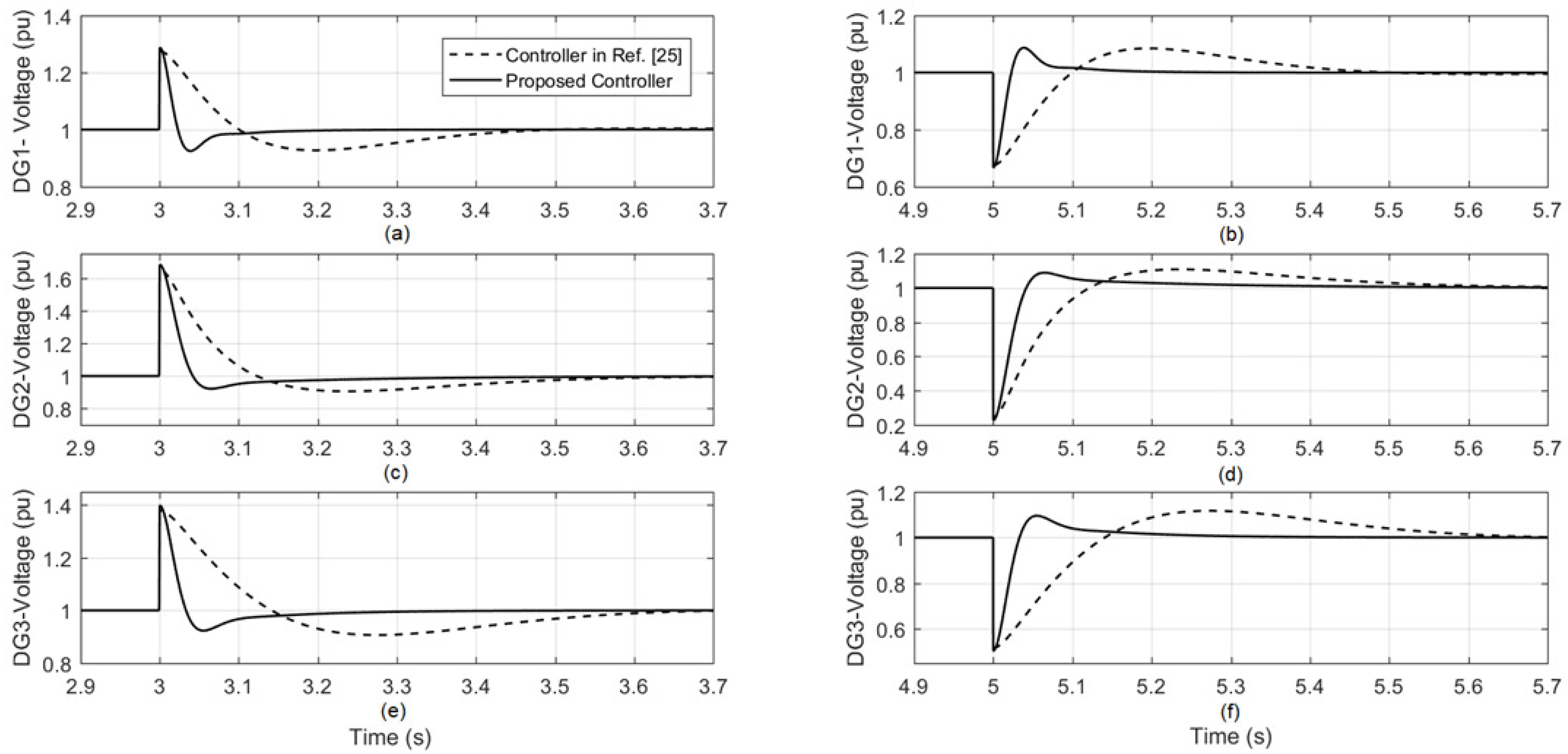
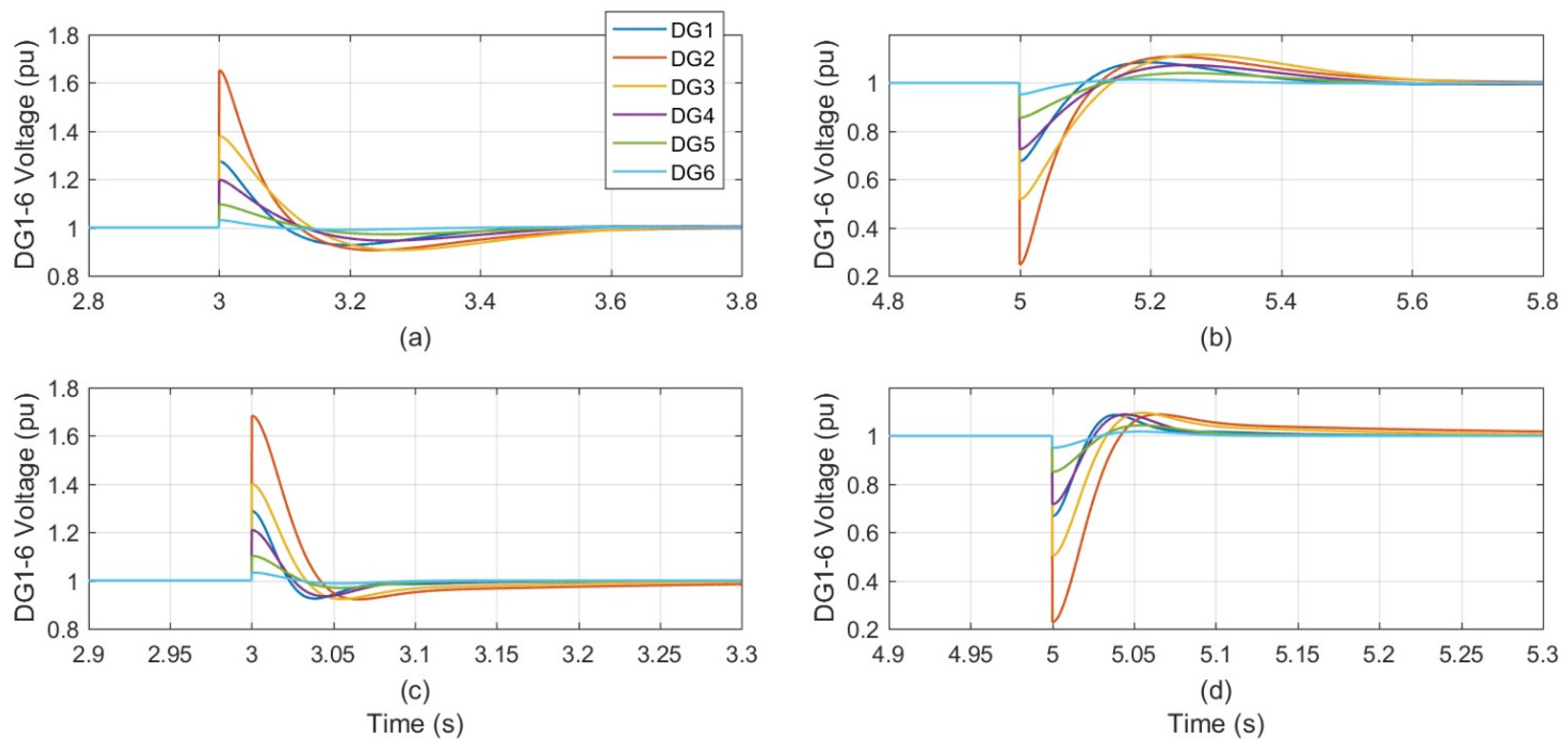
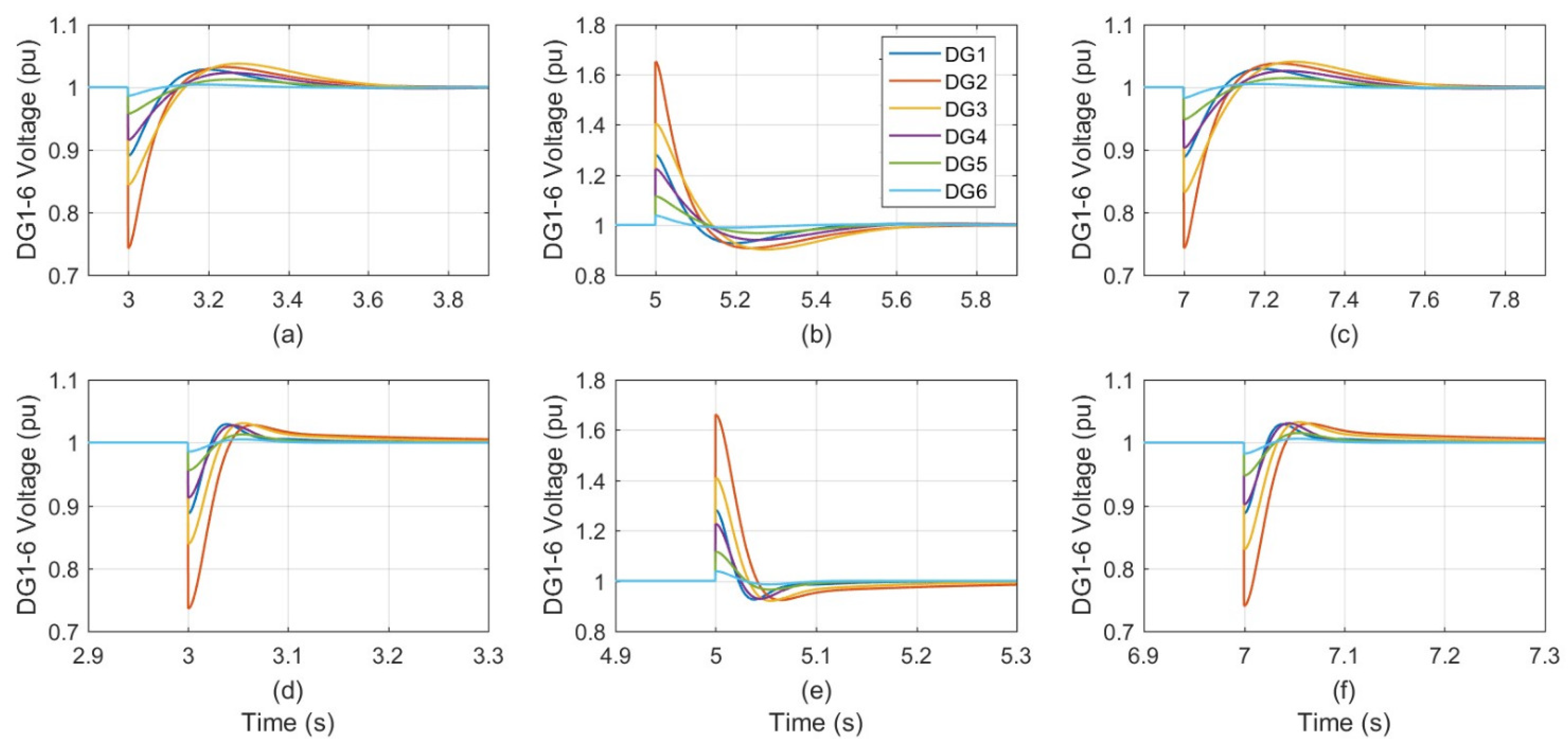
5.1. Case (1): Plug and Play (PnP) Potentials of DGs

Using a PnP functionality assessment configuration, the dynamic response of the proposed tracker is examined. This can be accomplished by plugging and unplugging a single DG from the MG system. Assume that DG “i” is isolated from the six-DG microgrid depicted in Figure 2. This equates to setting the x i vector to zero, or the A i j matrix set to equal zero. The possibilities for disconnecting any 6 DGs are summarized in Table 3.
DG2 is chosen for simulation from Table 3. At t = 3 s, DG2 is unplugged from the MG system and reconnects at t = 5 s. The three plots, on the left in Figure 3 and Figure 4, show the six DGs’ Point of Common Coupling (PCC) voltages during DG2 disconnection, and the three plots, on the right in Figure 3 and Figure 4, show the six DGs’ voltages at PCC when DG2 is restored back to the MG system. In both figures, the suggested controller for each DG is compared to the invariant-set controller utilized in [25], with a solid line for the proposed controller and dashed line for the invariant-set controller in [25].
The DG2 disconnection is highlighted by the significant overvoltage (over 1.6 p.u.) at PCC2 compared to other surrounding PCC overvoltages (always below 1.4 p.u.). Dually, the reconnection of DG2 is highlighted by the sudden voltage drop (below 0.3 p.u.) at PCC2, which is much deeper when compared to other surrounding PCC voltage drops (always above 0.5 p.u.). It is interesting to note that between the two DGs closer to DG2 with respect to other DGs, those are DG1 and DG3, the one that is more affected by overvoltage and undervoltage changes is DG3; this is due to the higher value of the line impedance of Z 23 with respect to Z 12 .
The results show that DG2’s PnP operation has no negative impact on the MG system’s stability. In addition, the six DGs in the MG system are strongly stable against the PnP configuration of DG2 without the need for further tracker retuning. The proposed tracker is over three times faster than the invariant-set controller used in [25].

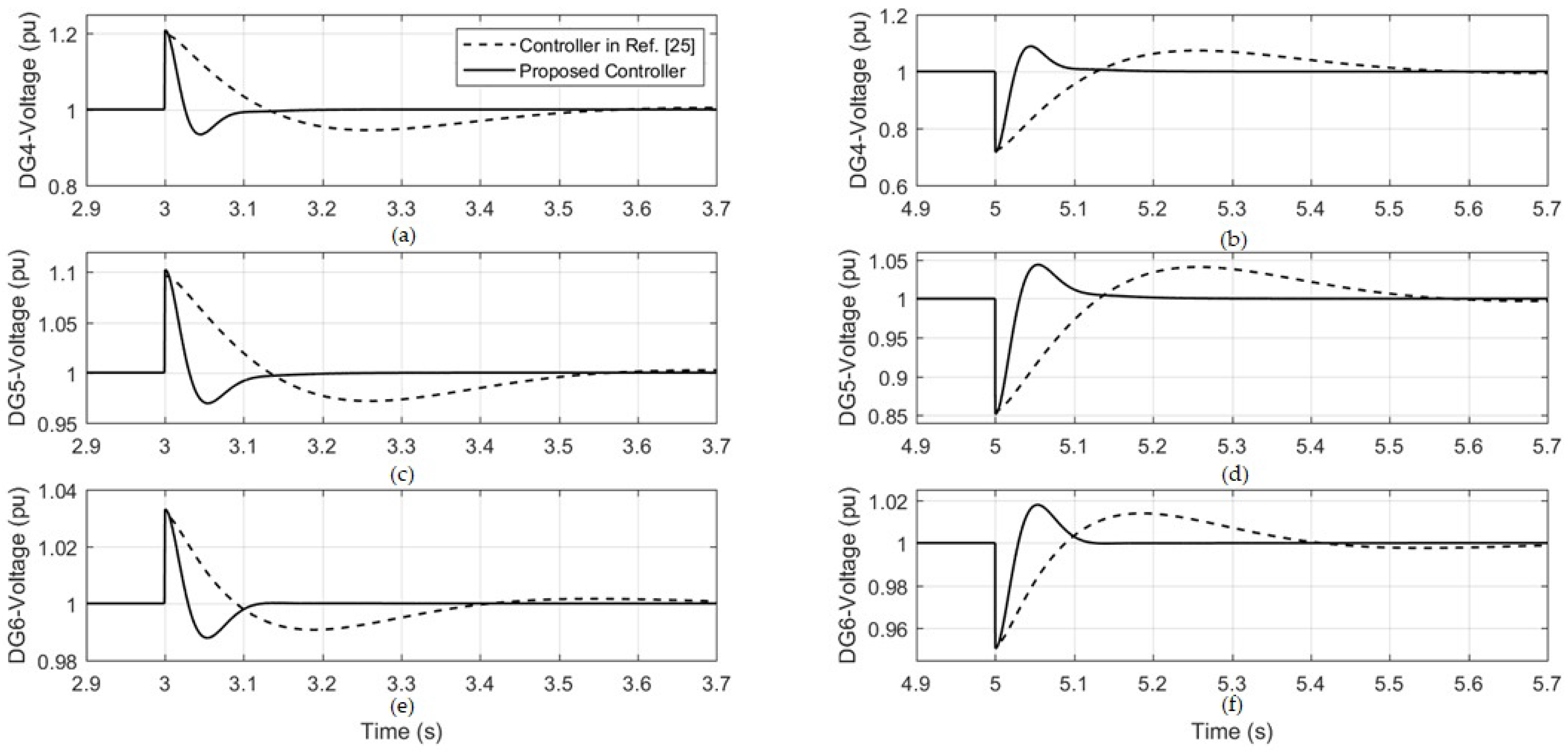
5.2. Case (2): Change in Distribution Line (DL) Parameter

In the DC-MG system, the DC-MG distribution line (DL) connecting the DGs has two parameters, R i j and L i j . Table 2 lists the DL parameters for each DG in Figure 2. When analyzing the robustness of a tracker in a DC-MG system, only changes in the resistive component in DL is considered a disturbance that must be rejected. The proposed controller is evaluated for ± 10 % in the parameter variation (say at R 34 ) as shown in Table 4.
Figure 5 and Figure 6 illustrate the DGs’ voltages when R 34 of DL is changed by ± 10 % . In comparison to the invariant-set controller employed in [25], the suggested trackers can handle this uncertainty precisely, and quickly, as demonstrated in Figure 5 and Figure 6; a dashed line is used for the invariant-set controller in [25] and a solid line for the proposed controller.

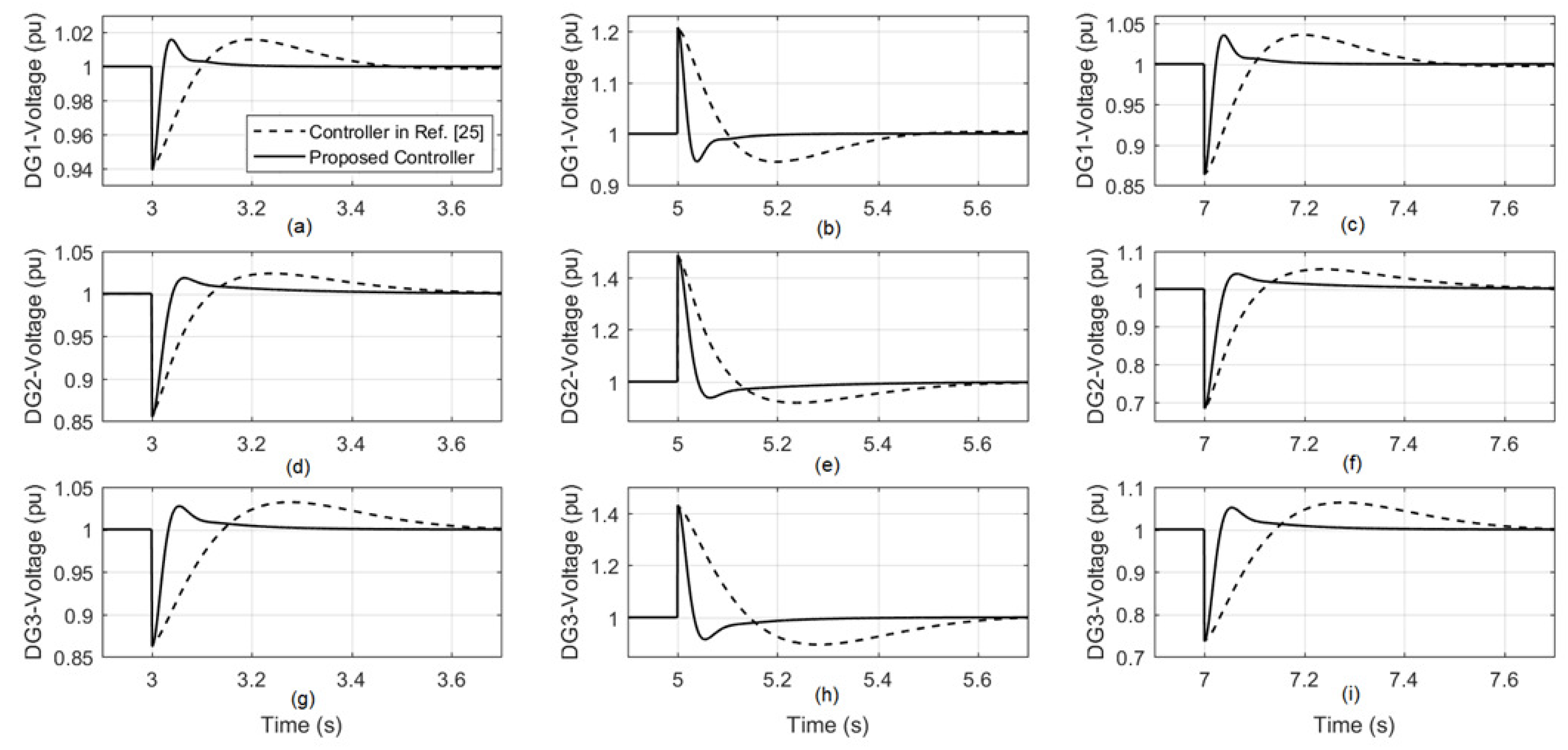
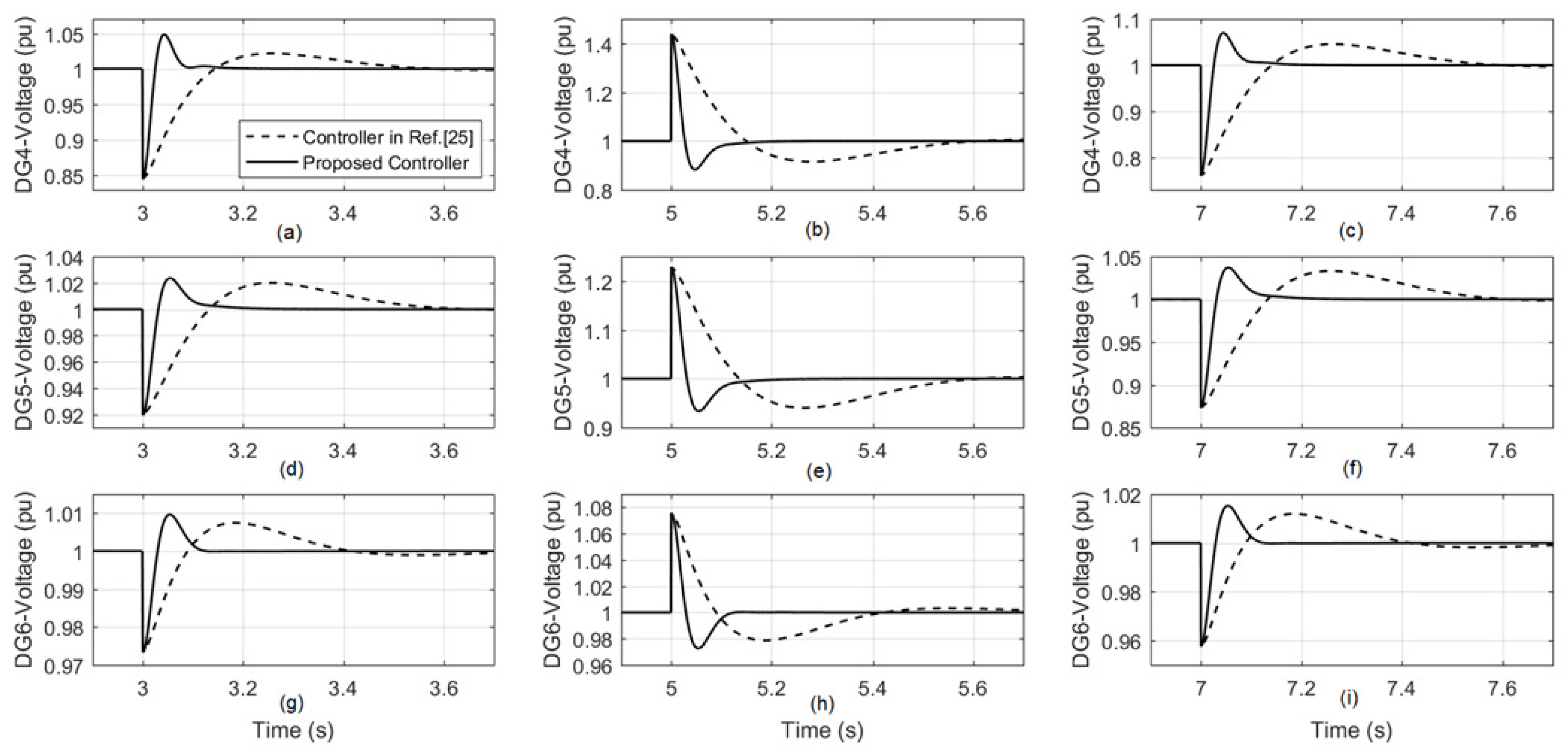
5.3. Case (3): Change in Load
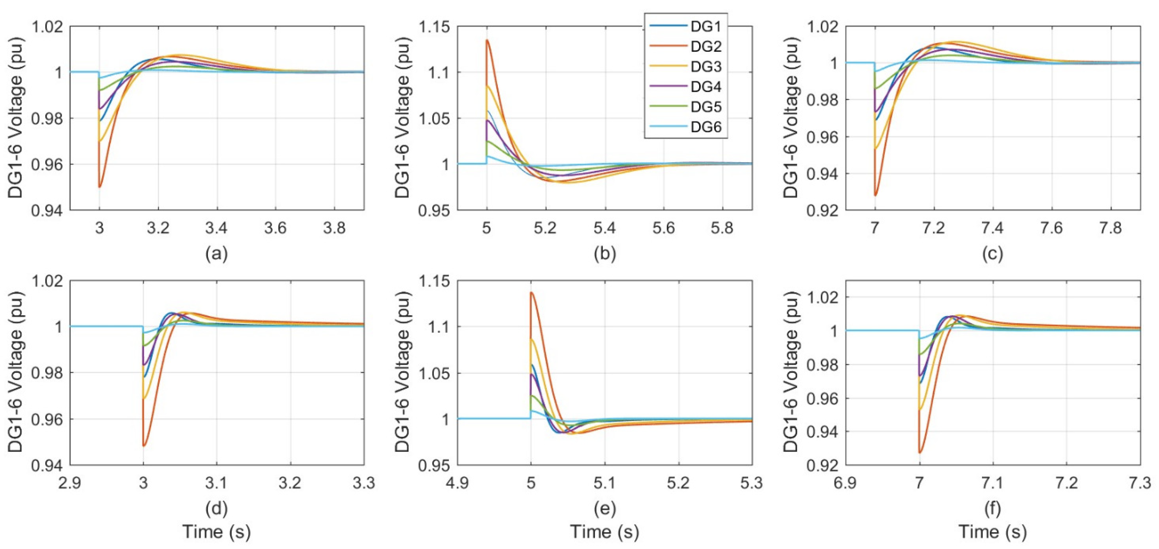
The proposed controllers are premeditated to abandon any load perturbation less than 10 % . Table 5 demonstrates how its practicability is evaluated under more extreme conditions ( 40 % on–off load variations beyond the design scope).
In this scenario, the suggested tracker’s swiftness will be evaluated by applying load fluctuations for one of the DGs contained inside the MG in the following manner: Table 1 illustrates the local load characteristics for each of the six DGs.

5.4. Scenario (1): A ± 10 % Change in DG2 Load

Table 5 displays the dynamic voltage responses of the six DGs under a 10 % load variation (Figure 7). Figure 7 depicts the six DGs’ load power during the same variations; the colors of the curves are blue for DG1, orange for DG2, yellow for DG3, violet for DG4, green for DG5, and cyan for DG6.
Figure 7 depicts the voltage response of the MG system when the R 2 load of DG2 is increased to 100 % . The response with the controller in [25] is shown in Figure 7a–c, with the proposed tracker in Figure 7d–f. The voltage response of the six DGs is given, respectively, for the control of [25], and the proposed one in Figure 7a,d when R 2 changes from 100 % to 90 % , Figure 7b,e when R 2 changes from 90 % to 110 % , and Figure 7c,f when R 2 changes from 110 % to 100 % .

5.5. Scenario (2): A ± 40 % Change in DG2 Load

According to Table 5, the SIX DGs’ dynamic voltage responses during the ± 40 % load change are shown. Figure 8a–c displays the six DGs’ voltage, while R 2 at DG2 varies from 100 % to 60 % , from 60 % to 140 % , and from 140 % to 100 % , respectively, when the controller in [25] is used. The six DGs’ voltages are then shown in Figure 8d–f when R 2 , at DG2, changes from 100 % to 60 % , from 60 % to 140 % , and from 140 % to 100 % , respectively, when the proposed tracker is employed. The colors of the curves are blue for DG1, orange for DG2, yellow for DG3, violet for DG4, green for DG5, and cyan for DG6.

5.6. Scenario (3): DG2 Load Connecting and Disconnecting (ON/OFF)

In practice, the DG local load is engaged and disengaged, for illustration, when the batteries of electric vehicles are being charged and discharged. Accept that the load resistance is equal to or close to infinity to represent a detached local load of one DG. At t = 3 s, the load resistance R 2 at DG2 of the MG is detached (turned off), and at t = 5 s, it is reconnected (turned on) to its starting value ( 100 % ). When controllers of [25] are used, Figure 9a,b shows the response under the connecting and disconnecting (on/off) load of DG2. Figure 9a depicts the six DGs’ PCC voltage after the DG2 load is attached, whereas Figure 9b depicts the six DGs’ PCC voltage after the DG2 load is disconnected ( 100 % ) to the MG. The colors of the curves are blue for DG1, orange for DG2, yellow for DG3, violet for DG4, green for DG5, and cyan for DG6. Figure 9c,d depicts the loading and unloading (on/off) of DG2 when the suggested trackers are utilized. The results in Figure 5, Figure 6, Figure 7, Figure 8 and Figure 9 demonstrate the resilience and swiftness of the response compared to those utilized in [25] against load changes. It is worth noting that load and DL alterations in a location other than those listed above produce comparable results.
Note that the proposed state feedback PI is much better than the state feedback I ellipsoidal design [25]. The latter outperforms many methods given in [25], see Table 6 (the percentage of the steady-state error is equal to zero for all the reported cases for both the proposed controller and the one in [25]).
As shown in Table 6, the percentage of overvoltages is more pronounced in case 5.1 with respect to all other cases, for the first scenario, when DG2 is unplugged from the MG. This overvoltage occurs because the entire DG2 is removed from the system, and the overshoot is particularly visible at PCC2, where DG2 is detached. The overvoltage values are close to 67% for both controllers in the proposed controller and the one in [25], whereas Table 6 shows that the rising and settling times are much shorter for the proposed controller.
The persistence of an overvoltage or undervoltage condition for a period exceeding hundreds of milliseconds can lead to the activation of the protection systems present in power lines. Therefore, having a control system that, following a change in the line parameters or the distributed generators or the loads connected to the PCC, has a very rapid response, both in terms of rising time and settling time, constitutes a very important aspect to guarantee good coordination with the protection systems and therefore allows the good functioning of the MG.
Notably, the voltage at PCC3 was particularly overshot by the removal of DG2. For the proposed controller, the overvoltage of DG3 was limited to within 40%, whereas for the controller in [25], the overvoltage reached almost 90%. This trend proves that the proposed controller, besides being faster, also shows a higher stability transient behavior.
The overvoltage is also very pronounced when the resistance R 34 of the distribution line between DG3 and DG4 is increased from 90% to 110% (case 5.2, second scenario), which limits the overshoot of the voltage slightly over 40%, similar to the response of the controller in [25]. This behavior shows that the voltage of the MG is very sensitive to changes in the line distribution parameters. In this scenario, the rising time of the proposed controller was five times faster than that of the controller in [25], and the settling time was twice as fast.
The load changes in both cases 5.4 and 5.5 do not show remarkable overvoltages. In Scenario 5.6, when the load is completely linked back after having been detached, the overvoltage is quite remarkable, reaching a value of approximately 11% for the proposed controller and 12% for the controller in [25], and the rising and settling times are always shorter for the proposed controller.

6. Conclusions

This paper proposed a passivity-based voltage tracker for a DC-MG. The suggested design develops a new sufficient condition in terms of a bilinear matrix inequality (entirely different from the existing ones [5,22,25]). The decentralized control is achieved by rejecting the external disturbance on each subsystem by minimizing the size of the attracting ellipsoid. The proposed control is fully decentralized and allows the removal and addition of DGs in a PnP operation. It is also robust against uncertainties in lines and loads. Asymptotic stability and good damping properties were deduced in simulation results for DC voltage control and improvements compared to a controller already present in the literature were presented; the proposed tracker was shown to be over three times faster than the invariant-set controller used in the literature. The limitation of the proposed design is the need to solve bilinear matrix equations which need software that is not free to download, whereas the proposed control can be applied to some nonlinear systems modeled by quasi-Lipschitz approximation.
Future research studies will consider more complex load models, e.g., electric vehicles, and multi-objectives like current and power sharing. In more detail, future works can extend the use of the proposed method to coordinate actions among multiple DGs to compensate for power quality issues, particularly if the microgrid was connected to the main distribution network since most industrial plants supply nonlinear loads. Moreover, the proposed method can be well suited to solving the design of optimization problem of islanded microgrid systems using solar photovoltaics, micro-hydropower, and wind turbines, battery storage, and electric vehicles.

Author Contributions

Conceptualization, A.S.P., H.M.S., H.A. and E.H.E.B.; methodology, A.S.P., H.M.S., H.A., E.H.E.B. and M.D.S.; software, A.S.P., H.M.S., H.A. and E.H.E.B.; validation, A.S.P., H.M.S., H.A., E.H.E.B. and M.D.S.; formal analysis, A.S.P., H.M.S., H.A., E.H.E.B. and M.D.S.; investigation, A.S.P., H.M.S., H.A., E.H.E.B. and M.D.S.; resources, E.H.E.B. and M.D.S.; data curation, A.S.P., H.M.S., H.A., E.H.E.B. and M.D.S.; writing—original draft preparation, A.S.P., H.M.S., H.A., E.H.E.B. and M.D.S.; writing—review and editing, A.S.P., H.M.S., H.A., E.H.E.B. and M.D.S.; visualization, A.S.P., H.M.S., H.A., E.H.E.B. and M.D.S.; supervision, A.S.P., H.M.S., H.A., E.H.E.B. and M.D.S. All authors have read and agreed to the published version of the manuscript.

Funding

This research received no external funding.

Data Availability Statement

Data is contained within the article.

Conflicts of Interest

The authors declare no conflicts of interest.

Appendix A

Appendix A.1. Proof Lemma 1 (the Extended Version of η-Dissipativity Property)

Suppose ∀ t t 0 0 , the next inequality holds
d d t V 1 x t 2 w t z t + 2 η w t w t 0 V 1 x = x P 1 x , P 1 = P 1 > 0
Defining β t : = 2 w t z t + 2 η w t w t , it can be represented as
d d t V 1 x t β t
the solution of which is
V x t V x t 0 2 t = t 0 t w τ z τ d τ + 2 η t = t 0 t w τ w τ d τ 0
implying (26). To finish the proof it is sufficient to note that property (A1) is fulfilled if the LMI (25) is valid.

References

  1. Fan, L. Control and Dynamics in Power Systems and Microgrids; Taylor & Francis Group: Boca Raton, FL, USA, 2017. [Google Scholar]
  2. Bevrani, H.; Francois, B.T.I. Microgrid Dynamics and Control; John Wiley & Sons, Inc.: New York, NY, USA, 2017. [Google Scholar]
  3. De Souza, A.C.Z.; Castilla, M. Microgrids Design and Implementation; Springer Nature Switzerland, AG: Cham, Switzerland, 2019. [Google Scholar]
  4. Sallam, A.; Malik, O. Electric Distribution Systems; John Wiley & Sons: New York, NY, USA, 2019. [Google Scholar]
  5. Bayoumi, E.; Soliman, M.; Soliman, H.M. Disturbance-rejection voltage control of an isolated microgrid by invariant sets. IET Renew. Power Gener. 2020, 14, 2331–2339. [Google Scholar] [CrossRef]
  6. Mehdi, M.; Saad, M.; Jamali, S.Z.; Kim, C.H. Output-feedback based robust controller for uncertain DC islanded microgrid. Trans. Inst. Meas. Control. 2020, 42, 1239–1251. [Google Scholar] [CrossRef]
  7. Mahmoud, M.S. Microgrid: Advanced Control Methods and Renewable Energy System Integration; Elsevier: Amsterdam, The Netherlands, 2016. [Google Scholar]
  8. Li, X.; Liu, B.; Zhuo, F.; Ning, G. A novel control strategy based on DC bus signaling for DC micro-grid with photovoltaic and battery energy storage. In Proceedings of the In 2016 China International Conference on Electricity Distribution (CICED), Xi’an, China, 10–13 August 2016; IEEE: Toulouse, France, 2016; pp. 1–5. [Google Scholar]
  9. Kumar, R.; Pathak, M.K. Distributed droop control of dc microgrid for improved voltage regulation and current sharing. IET Renew. Power Gener. 2020, 14, 2499–2506. [Google Scholar] [CrossRef]
  10. Bharathi, G.; Kantharao, P.; Srinivasarao, R. Fuzzy logic control (FLC)-based coordination control of DC microgrid with energy storage system and hybrid distributed generation. Int. J. Ambient. Energy 2021, 43, 4255–4271. [Google Scholar] [CrossRef]
  11. Ochoa, D.; Martinez, S.; Arévalo, P. A Novel Fuzzy-Logic-Based Control Strategy for Power Smoothing in High-Wind Penetrated Power Systems and Its Validation in a Microgrid Lab. Electronics 2023, 12, 1721. [Google Scholar] [CrossRef]
  12. Kramer, O. Genetic algorithms. In Genetic Algorithm Essentials; Springer: Cham, Switzerland, 2017. [Google Scholar]
  13. Kler, D.; Kumar, V.; Rana, K.P. Optimal integral minus proportional derivative controller design by evolutionary algorithm for thermal-renewable energy-hybrid power systems. IET Renew. Power Gener. 2019, 13, 2000–2012. [Google Scholar] [CrossRef]
  14. Che, L.; Shahidehpour, M. DC microgrids: Economic operation and enhancement of resilience by hierarchical control. IEEE Trans. Smart Grid 2014, 5, 2517–2526. [Google Scholar]
  15. Wang, P.; Xiao, J.; Setyawan, L.; Jin, C.; Hoong, C.F. Hierarchical control of active hybrid energy storage system (HESS) in DC microgrids. In Proceedings of the In 9th IEEE Conference on Industrial Electronics and Applications, Hangzhou, China, 9–11 June 2014; IEEE: Toulouse, France, 2014; pp. 569–574. [Google Scholar]
  16. Tavakoli, S.D.; Khajesalehi, J.; Hamzeh, M.; Sheshyekani, K. Decentralised voltage balancing in bipolar dc microgrids equipped with trans-z-source interlinking converter. IET Renew. Power Gener. 2016, 10, 703–712. [Google Scholar] [CrossRef]
  17. Olivares, D.E.; Mehrizi-Sani, A.; Etemadi, A.H.; Cañizares, C.A.; Iravani, R.; Kazerani, M.; Hatziargyriou, N. Trends in microgrid control. IEEE Trans. Smart Grid 2014, 5, 1905–1919. [Google Scholar] [CrossRef]
  18. Islam, S.; Agarwal, S.; Shyam, A.B.; Ingle, A.; Thomas, S.; Anand, S.; Sahoo, S.R. Ideal current-based distributed control to compensate line impedance in DC microgrid. IET Power Electron. 2018, 11, 1178–1186. [Google Scholar] [CrossRef]
  19. Bidram, A.; Nasirian, V.; Davoudi, A.; Lewis, F.L. Cooperative Synchronization in Distributed Microgrid Control; Springer International Publishing: Cham, Switzerland, 2017. [Google Scholar]
  20. Tucci, M.; Riverso, S.; Vasquez, J.C.; Guerrero, J.M.; Ferrari-Trecate, G. Decentralized scalable approach to voltage control of DC islanded microgrids. IEEE Trans. Control. Syst. Technol. 2016, 24, 1965–1979. [Google Scholar] [CrossRef]
  21. Firdaus, A.; Mishra, S. Auxiliary signal-assisted droop-based secondary frequency control of inverter-based PV microgrids for improvement in power sharing and system stability. IET Renew. Power Gener. 2019, 13, 2328–2337. [Google Scholar] [CrossRef]
  22. Nahata, P.; Soloperto, R.; Tucci, M.; Martinelli, A.; Ferrari-Trecate, G. A passivity-based approach to voltage stabilization in DC microgrids with ZIP loads. Automatica 2020, 113, 108770. [Google Scholar] [CrossRef]
  23. Hernández-Guzmán, V.M.; Silva-Ortigoza, R.; Orrante-Sakanassi, J.A. Energy-Based Control of Electromechanical Systems A Novel Passivity-Based Approach; Springer: Cham, Switzerland, 2021. [Google Scholar]
  24. Ortega, R.; Romero, J.G.; Borja, P.; Donaire, A. PID Passivity-Based Control of Nonlinear Systems with Applications; John Wiley: New York, NY, USA, 2021. [Google Scholar]
  25. Soliman, H.M.; Bayoumi, E.H.; El-Sheikhi, F.A.; Ibrahim, A.M. Ellipsoidal-Set Design of the Decentralized Plug and Play Control for Direct Current Microgrids. IEEE Access 2021, 9, 96898–96911. [Google Scholar] [CrossRef]
  26. Poznyak, A.; Polyakov, A.; Azhmyakov, V. Attractive Ellipsoids in Robust Control; Birkhauser: Boston, MA, USA, 2014. [Google Scholar]
  27. Cucuzzella, M.; Cucuzzella, K.; Kosaraju, K.; Kosaraju, M.; Scherpen, M.A. Distributed Passivity-Based Control of DC Microgrids. In Proceedings of the American Control Conference (ACC), Philadelphia, PA, USA, 10–12 July 2019. [Google Scholar]
  28. Malan, A.; Jané-Soniera, P.; Strehle, F.; Hohmann, S. Passivity-based power sharing and voltage regulation in DC microgrids with un-actuated buses. Syst. Control. 2023, 2301, 13533. [Google Scholar]
  29. Khalil, H.K. Nonlinear Systems; Pearson: San Antonio, TX, USA, 2014. [Google Scholar]
  30. Loranca-Coutiño, J.; Mayo-Maldonado, J.C.; Escobar, G.; Maupong, T.M.; Valdez-Resendiz, J.E.; Rosas-Caro, J.C. Data-Driven Passivity-Based Control Design for Modular DC Microgrids. IEEE Trans. Ind. Electron. 2022, 69, 2545–2556. [Google Scholar] [CrossRef]
  31. Magaldi, G.; Serra, F.M. andde Angelo, C.; Montoya, O.; Giral-Ramírez, D. Voltage Regulation of an Isolated DC Microgrid with a Constant Power Load: A Passivity-based Control Design. Electronics 2021, 10, 2085. [Google Scholar] [CrossRef]
  32. Sadabadi, M.S.; Shafiee, Q.; Karimi, A. Plug-and-play robust voltage control of DC microgrids. IEEE Trans. Smart Grid 2017, 9, 6886–6896. [Google Scholar] [CrossRef]
  33. IEEE Standards Association. IEEE Std 1159-IEEE Recommended Practice for Monitoring Electric Power Quality; IEEE: Toulouse, France, 2009. [Google Scholar]
  34. Awad, H.; Bayoumi, E.; Soliman, H.; De Santis, M. Robust Tracker of Hybrid Microgrids by the Invariant-Ellipsoid Set. Electronics 2021, 10, 1794. [Google Scholar] [CrossRef]
Figure 1. Two DGs form a DC microgrid.
Energies 17 01529 g001
Figure 2. A 6 DG islanded DC microgrid.
Energies 17 01529 g002
Figure 3. Voltage behavior of an MG system with PnP capabilities: dashed curve for controller in [25], solid curve for the proposed controller. Voltage dynamic behaviors of DG1-3 when DG2 is unplugged (three plots on the left, (a,c,e)). DG1-3 voltage dynamic responses when DG2 is linked back (three plots on the right, (b,d,f)).
Energies 17 01529 g003
Figure 4. Voltage performance of the MG system with PnP functionality: dashed curve for controller in [25], solid curve for the proposed controller. When DG2 is disconnected, DG4-6 voltage dynamic responses (three plots on the left, (a,c,e)). DG4-6 voltage dynamic responses when DG2 is linked back (three plots on the right, (b,d,f)).
Energies 17 01529 g004
Figure 5. The voltage performance of the proposed MG system due to the change in R 34 of the DL: dashed curve for controller in [25], solid curve for the proposed controller. Starting from the top down, DG1 (ac), DG2 (df), and DG3 (gi) voltages during R 34 change from 100% to 90%, from 90% to 110%, and from 110% to 100%, with respect to the three plots moving from left to right, respectively.
Energies 17 01529 g005
Figure 6. The voltage performance of the proposed MG system due to the change in R 34 of the distribution line: dashed curve for controller in [25], solid curve for the proposed controller. Starting from the top down, DG4 (ac), DG5 (df), and DG6 (gi) voltages during R 34 change from 100% to 90%, from 90% to 110%, and from 110% to 100%, with respect to the three plots moving from left to right, respectively.
Energies 17 01529 g006
Figure 7. This shows the 6 DG voltages when R 2 at DG2 varies from 100 % to 90 % , from 90 % to 110 % , and from 110 % to 100 % , respectively, when the invariant-set controller in [25] and the proposed controller are used. The response with the controller in [25] is shown in (ac), with the proposed tracker in (df); the code of colors is DG1, DG2, DG3, DG4, DG5, and DG6.
Energies 17 01529 g007
Figure 8. The recommended MG arrangement voltage responses when the R2 load parameter of DG2 is changed by ± 40 % ; (ac) for the controller in [25], (df) for the suggested tracker: the code of colors is DG1, DG2, DG3, DG4, DG5, and DG6. (a,d) Six DG voltages for turning from 100 % to 60 % in R 2 , (b,e) six DG voltages for turning from 60 % to 140 % in R 2 , (c,f) six DG voltages for turning from 140 % to 100 % in R 2 .
Energies 17 01529 g008
Figure 9. Dynamic response of the MG under load disconnection and reconnection: (a,b) with the controller from [25] and (c,d) with the suggested tracker; the code of colors is DG1, DG2, DG3, DG4, DG5, and DG6. (a,b) Dynamic response of DGs’ voltages when DG2 load is detached (off) and reattached (on), according to [25]. (c,d) Dynamic response of DGs’ voltages when DG2 load is detached (off) and reattached (on), according to the proposed algorithm.
Energies 17 01529 g009
Table 1. Parameters of the microgrid system.
DG s Buck Converter Resistance R t ( Ω )Buck Converter Inductance L t (mH)Shunt Capacitor C t (mF)Load Parameter R ( Ω )Rated Power (W)
DG 1 7.22072.225.0160.01200
DG 2 14.440144.032.080.0600
DG 3 10.830108.025.0120.0900
DG 4 7.22072.2030.0160.01200
DG 5 14.400144.018.0100.0800
DG 6 10.830108.012.0120.0900
DC busvoltage: V d c = 100 V
Switchingfrequency: f s w = 40 kHz
Nominalfrequency: f 0 = 50 Hz
Table 2. Distribution line (DL) parameters.
Line Impedance Z ij Line Resistance per Unit Length r ij ( Ω /m)Cable Length (m)Line Resistance R ij ( Ω )Line Inductance per Unit Length l ij ( μ H/m)Line Inductance L ij ( μ H)
Z 12 0.05018091.8324
Z 23 0.050240121.8432
Z 34 0.050300151.8540
Z 45 0.050240121.8432
Z 56 0.05026413.21.8475.2
Table 3. Zero matrix detection in zone DG disconnection.
Zone DG DisconnectionZero Matrix Detection
1 DG 1 A 21
2 DG 2 A 12 , A 22
3 DG 3 A 23 , A 43
4 DG 4 A 34 , A 54
5 DG 5 A 45
Table 4. Percentage change for R 34 vs. time.
Time (s) R 34 (±10% Change)
0–3100%
3–590%
5–7110%
>7100%
Table 5. Time/percentage change test.
Time (s)Load Change ( ± 10 % )Load Change ( ± 40 % )100% On/Off Load
0–3100%100%On
3–590%60%Off
5–7110%140%On
>7100%100%Off
Table 6. Comparison between the proposed controller and controller in [25].
# of CasesScenariosOccurrence/TypeThis ControlControl in [25]
DG1DG2DG3DG4DG5DG6DG1DG2DG3DG4DG5DG6
Unplug%Overshoot29.3066.7039.80 21.3010.203.6229.2066.5089.50 21.109.933.54
DG2Rise Time(s)0.0270.0340.029 0.0270.0280.0290.1020.1130.120 0.0920.0940.112
5.1 Settling Time(s)0.1030.2020.187 0.1010.1160.1010.3470.3530.367 0.350.3510.392
Link%Overshoot9.349.769.56 8.564.831.929.2910.8211.73 8.214.781.78
backRise Time(s)0.0280.0350.031 0.0280.0290.0310.1030.1090.011 0.9030.9220.983
5.1DG2Settling Time(s)0.1040.2010.184 0.1080.1210.1030.3520.3610.371 0.3490.3480.389
R 34 %Overshoot1.872.353.25 5.032.311.091.902.653.67 3.780.210.87
from 100%Rise Time(s)0.0120.0220.024 0.0290.0210.1980.1150.1230.174 0.1890.1650.115
5.2to 90%Settling Time(s)0.0870.1150.187 0.1930.1050.0950.3970.3560.361 0.3520.3510.394
R 34 %Overshoot20.946.7241.74 41.5623.427.2320.8645.5140.89 41.0223.287.09
from 90%Rise Time(s)0.0140.0210.024 0.0240.0230.0190.0930.1220.151 0.1510.1560.102
5.2to 110%Settling Time(s)0.1090.2130.236 0.2310.2410.1570.4130.5720.592 0.5900.5820.392
R 34 %Overshoot3.7825.3416.893 7.9814.1051.7453.9657.2048.021 6.7213.8741.627
from 110%Rise Time(s)0.0130.0210.024 0.0250.0250.1780.0970.1230.156 0.1760.1650.137
5.2to 100%Settling Time(s)0.0890.2010.231 0.2410.0240.0150.4080.5620.595 0.5210.5320.371
R 2 %Overshoot0.4720.6450.673 0.4810.2450.1310.6230.8120.915 0.6140.4320.213
from 100%Rise Time(s)0.0080.0540.032 0.0080.0070.0040.1250.1670.171 0.1230.1120.080
5.4to 90%Settling Time(s)0.0880.2070.201 0.1020.0750.0530.4530.4640.561 0.5510.5570.352
R 2 %Overshoot0.2870.3720.415 0.2840.1340.0830.3080.4720.486 0.3210.2370.106
from 100%Rise Time(s)0.0320.0430.094 0.0830.0620.0210.0730.1640.189 0.1830.1670.158
5.5to 60%Settling Time(s)0.1740.2780.289 0.2910.1570.1050.4520.5920.601 0.5830.4320.377
Load is%Overshoot6.4710.8311.34 6.893.832.356.3212.1512.73 6.774.322.11
attachedRise Time(s)0.0310.0470.042 0.0370.0310.0340.9410.1050.131 0.1450.0970.082
5.6(on)Settling Time(s)0.1340.2550.247 0.1370.0810.0630.4150.5540.582 0.5420.4130.187
Disclaimer/Publisher’s Note: The statements, opinions and data contained in all publications are solely those of the individual author(s) and contributor(s) and not of MDPI and/or the editor(s). MDPI and/or the editor(s) disclaim responsibility for any injury to people or property resulting from any ideas, methods, instructions or products referred to in the content.

