Probabilistic Design Methods for Gust-Based Loads on Wind Turbines

Abstract

The IEC 61400-1 standard specifies design load cases (DLCs) to be considered in the design of wind turbine structures. Specifically, DLC 2.3 considers the occurrence of a gust while the turbine shuts down due to an electrical fault. Originally, this load case used a deterministic wind event called the extreme operating gust (EOG), but the standard now also includes an approach for calculating the extreme response based on stochastic simulations with turbulent wind. This study presents and compares existing approaches with novel probabilistic design approaches for DLC 2.3 based on simulations with turbulent wind. First, a semiprobabilistic approach is proposed, where the inverse first-order reliability method (iFORM) is used for the extrapolation of the response for electrical faults occurring at a given rate. Next, three probabilistic approaches are formulated for the calculation of the reliability index, which differs in how the aggregation is performed over wind conditions and whether faults are modeled using a Poisson distribution or just by the rate. An example illustrates the methods considering the tower fore-aft bending moment at the tower base and shows that the approach based on iFORM can lead to reductions in material usage compared to the existing methods. For reliability assessment, the probabilistic approach using the Poisson process is needed for high failure rates, and the reliabilities obtained for designs using all semiprobabilistic methods are above the target level, indicating that further reductions may be obtained via the use of probabilistic design methods.

1. Introduction

As of 2021, the total global installed capacity of offshore and onshore wind energy had reached more than 800 GW [1]. Turbines have also expanded in size, with the new Vestas V236-15.0 MW offshore prototype having a rotor diameter of 236 m. For a typical land-based 600 MW reference wind farm, with 75 wind turbines that are 8 MW each, the turbine and substructure contribute to over 75% of the capital expenditure (CAPEX) [2]. For an offshore fixed-bottom wind farm with similar capacity, this value is around 47% of the CAPEX.

Wind turbine structures are generally designed using the design load cases (DLCs) defined in the IEC 61400-1 design standard [3]. The load cases specify the wind climate and operational conditions for which the turbine structures are to be designed to sustain, including extreme wind speeds, extreme loads during normal operation, start-ups, shutdowns, and faults in the electrical systems. Additionally, fatigue load cases are defined [4]. For offshore wind turbines, the DLCs also specify the modeling of waves and currents [5].

The load conditions in IEC 61400-1 [3] are generally derived using statistical approaches [6] and are divided into normal and abnormal conditions, where abnormal conditions are used together with a lower safety factor to target an annual reliability index $\beta$ equal to 3.3 [7]. The characteristic load value for load cases with a normal safety factor typically has a 50-year return period. In some load cases (e.g., DLC 1.1), the 50-year load value is obtained by extrapolation of the response in normal wind conditions, and, in other load cases (e.g., DLC 1.3, 3.2, 4.2), the extreme response is obtained by running simulations with extreme environmental conditions found by extrapolation. For load cases with electrical faults or other events (such as start-up), the rate of faults/events is considered in the extrapolation. More-frequent events are combined with rarer environmental conditions and vice versa to achieve the required combined return period.

As an alternative to the traditional deterministic/semiprobabilistic approach used in IEC 61400-1, probabilistic approaches can be used for the design [8,9,10] and assessment [11] of wind turbines by explicitly considering the uncertainties present in the models, materials, and loads [12]. A reduction in uncertainties can be achieved by making use of data from measurement campaigns, operational monitoring, and tests. The application of probabilistic design methods for wind turbines can potentially deliver cost reductions through detailed modeling of the load cases that drive the design [13]. Currently, a technical specification on probabilistic design measures for wind turbines, IEC TS 61400-9 [14], is being developed. IEC TS 61400-9, on probabilistic design measures, aims to provide models and methods for more detailed design procedures in terms of probabilistic modeling.

The focus of the present work was DLC 2.3, which considers the combination of an electrical fault with a strong gust. In existing studies, the statistical characterization of extreme gusts based on measured data has been investigated [15,16], as has the implementation of extreme gusts in simulations with a turbulent wind field using constrained simulation [17,18]. However, since faults are quite rare, it is not likely that they happen during an extreme 50-year gust. Instead, the gust to be combined with an electrical fault should be chosen to achieve a 50-year response value also considering the rate of faults.

IEC 61400-1:2019 [3] includes two approaches for load assessment for DLC 2.3: using a deterministic wind field event called extreme operating gust (EOG) and using stochastic simulations using the normal turbulence model (NTM). In both cases, the underlying assumption is that the occurrence of the fault event and the gust are independent. The EOG gust has the shape of a Mexican hat and its current form was introduced in IEC 61400-1:2005 [19]. Its magnitude was determined using the Kaimal turbulence model as the maximum gust occurring in combination with a start-up or shut-down condition (DLC 3.2 and 4.2) with a recurrence period of 50 years [20,21]. In DLC 2.3, the same gust is combined with electrical fault events, and since electrical faults are rarer events than start-ups and shut-downs, the safety factor for abnormal events is used.

The alternative approach for DLC 2.3 was introduced in IEC 61400-1:2019 [3]. Here, stochastic simulations are performed using normal turbulence conditions (the NTM model), and the characteristic response value is obtained as the mean plus three standard deviations of the extreme responses extracted from the stochastic simulations. The inverse first-order reliability method (iFORM), was used to derive the procedure for the calculation of the extreme response having a 50-year return period [22]. iFORM [23] has been widely used to generate environmental contours for combinations of, for instance, the mean wind speed at hub height and the standard deviation of the mean wind speed having a given return period [24,25]. For example, the ETM model was derived to obtain combinations of mean wind speeds and the turbulence standard deviation corresponding to the 50-year environmental contour. However, for the derivation of the procedure for DLC 2.3, the response was also included as a variable, enabling iFORM to obtain the characteristic value of the response [22,26].

The present work aimed to make recommendations for IEC TS 61400-9 [14] on the use of probabilistic design approaches for design load case DLC 2.3 with electrical faults occurring during power production. We demonstrate how iFORM can be applied for the calculation of the response with a 50-year return period for DLC 2.3, and we compared the results to the existing methods in IEC 61400-1 [3]. We also report several probabilistic approaches for obtaining the annual failure probability for fault load cases, where the probability of occurrence of environmental conditions is used to weigh the extreme responses obtained for different conditions, and the rate of occurrence of faults is used. These include a novel approach, where a formulation based on the Poisson distribution makes the approach accurate for higher failure rates.

This paper is organized as follows: Section 2 describes three methods identified for deterministic/semiprobabilistic design in DLC 2.3 and describes three approaches for reliability assessment. Section 3 presents an example where the methods are applied for the tower bottom section of the NREL 5MW onshore wind turbine [27], and Section 4 presents the conclusions and recommendations.

2. Methods

This section describes the methods used in this study for design and assessments in DLC 2.3. All approaches are based on the assumption that the electrical failure and meteorological conditions are statistically independent. The design equation and limit state equation are formulated for yielding failure due to pure bending, but the methods described in this section can be applied to other limit states as well.

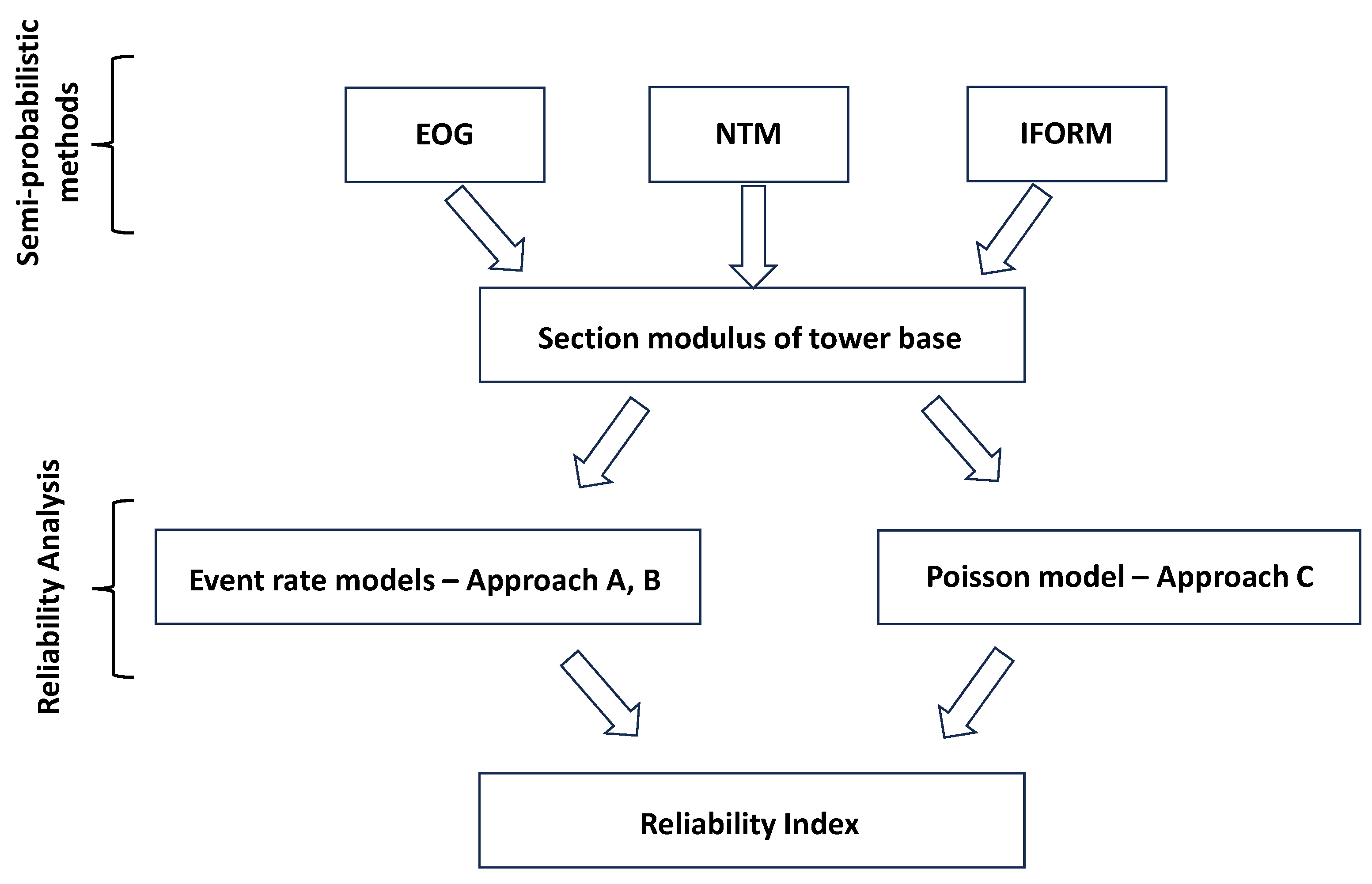
2.1. Semiprobabilistic Design Methods

In the semiprobabilistic/deterministic design methods, safety factors, and characteristic values are used in this design. Three semiprobabilistic design approaches for DLC 2.3 were included in the present study. The first two approaches are included in IEC 61400-1 [3] and are referred to as EOG and NTM, and the third approach is based on iFORM. All approaches are based on the assumption that the occurrence of electrical faults follows a Poisson process.

If the occurrence of an event follows a Poisson distribution with rate ${\lambda }_E$, and specific environmental conditions are exceeded a proportion $P_N$ of the time, the rate of the event happening while these conditions are exceeded is also a Poisson process. It has the rate

$$\lambda ={\lambda }_E·P_N$$

(1)

Consequently, to obtain a given return period $T_p=1/\lambda$, the environmental conditions should have an exceedance probability equal to

$$P_N=\frac{1}{{\lambda }_E{T}_p}$$

(2)

The design equation for yielding failure due to pure bending is given by

$$G=\frac{1}{{\gamma }_M}{f}_{yk}-{\gamma }_f\frac{M_k}{W}\ge 0$$

(3)

• ${\gamma }_M$ is the partial safety factor for the strength;
• $f_{yk}$ is the characteristic value of the steel’s yield strength;
• ${\gamma }_f$ is the partial safety factor for the load;
• $M_k$ is the characteristic moment load;
• W is the section modulus.

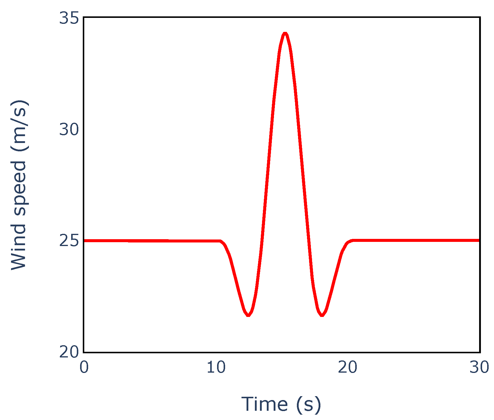
2.1.1. Extreme Operating Gust (EOG)

In the original formulation in IEC 61400-1, DLC 2.3 concerns the combination of an electrical fault (loss of electrical network) with the deterministic wind field event known as an EOG. The EOG is considered an abnormal event with a partial safety factor for the load of 1.1. The EOG is characterized by a sudden increase and then decrease in the wind speed over a short time interval following the shape of a Mexican sombrero [28]. Figure 1 shows an EOG profile for a hub-height speed equal to 25 m/s and a rotor diameter equal to 126 m, and the transient occurs over 10.5 s.

According to IEC 61400-1 [3], three hub-height wind speeds are to be considered: rated wind speed ±2 m/s and the cutout wind speed, and the timing of the electrical fault and gust should be chosen to obtain the worst loading. According to DNV-ST-0437:2021 [29], three combinations of the timing of the grid loss and the EOG are to be considered for each of the three hub-height wind speeds:

• Time of the lowest wind speed;
• Time of the highest gust acceleration;
• Time of the maximum wind speed.

According to IEC 61400-1, the hub-height gust magnitude is given by

$$V_{gust}=min\{1.35(V_{e1}-V_{hub});3.3(\frac{{\sigma }_1}{1+0.1\left(\frac{D}{{\Lambda }_1}\right)}\left)\right\}$$

(4)

where $V_{e1}$ is the extreme wind speed, with a recurrence period of 1 year. The turbulence standard deviation is given by the 90% quantile for the given hub-height wind speed:

$${\sigma }_1=I_{ref}(0.75V_{hub}+b);b=5.6\mathrm{m}/\mathrm{s}$$

(5)

$I_{ref}$ is the reference turbulence intensity, and $V_{hub}$ is the hub-height speed. The turbulence scale parameter is given by

$${\Lambda }_1=\left\{\begin{array}{cc}0.7z_{hub},\hfill & \mathrm{for}{z}_{hub}<60\mathrm{m}\hfill \\ 42\mathrm{m},\hfill & \mathrm{for}{z}_{hub}\ge 60\mathrm{m}\hfill \end{array}\right.$$

(6)

where $z_{hub}$ is the hub height.

The wind speed is obtained as a function of time t, at height z:

$$V(z,t)=\left\{\begin{array}{cc}V\left(z\right)-0.37V_{gust}sin(3\pi t/T)(1-cos(2\pi t/T)),\hfill & \mathrm{for}0\le t\le T\hfill \\ V\left(z\right),\hfill & \mathrm{otherwise}\hfill \end{array}\right.$$

(7)

where

$$\begin{array}{cc}\hfill V\left(z\right)& =V_{hub}{(z/z_{hub})}^{\alpha }\hfill \\ \hfill \alpha & =\mathrm{power}\mathrm{law}\mathrm{exponent}\left(0.2\right);\hfill \\ \hfill T& =10.5\mathrm{s};\hfill \end{array}$$

The factor 3.3 in Equation (4) was originally determined as the expected maximum gust occurring in combination with turbine start-up/shut-down conditions over a 50-year return period [20]. Using the Kaimal power spectrum, the distribution function was established for the increase in wind speed between two points in time, and the relevant exceedance probability $P_N$ was found using Equation (2), with ${\lambda }_E$ equal to the frequency of turbine shut-down/start-up per year [21].

2.1.2. Normal Turbulence Model (NTM)

IEC 61400-1 also suggests an alternative for the gust-based modeling of DLC 2.3. Here, DLC 2.3 is considered a normal event (the partial safety factor for the load is equal to 1.35), and stochastic wind conditions are simulated using the NTM. A fault in the electrical system (including grid loss) is introduced, and the maximum response after the introduction of the fault is recorded. This is illustrated in Figure 2, where the maximum bending moment is observed at a point in time soon after the introduction of the loss of grid (LoG) at 120 s for a hub-height wind speed of 25 m/s.

In order to obtain the characteristic response value, 12 simulations were performed at each wind speed between cut-in and cut-out. For each simulation, the extreme value of the response after the electrical fault has occurred was sampled. For a particular mean wind speed, the nominal extreme response was evaluated as the mean of the 12 sampled extreme responses plus three times the standard deviation of the samples, and the characteristic response was the extreme among the nominal extreme responses.

2.1.3. Inverse-FORM (iFORM)

The NTM procedure for the modeling of DLC 2.3 was originally derived using iFORM to obtain a combined return period of 50 years [22]. The factor three on the standard deviation was determined to give conservative estimates over a range of fault rates. For a specific application and fault rate, iFORM can instead be used directly for the estimation of the extreme response with a 50-year return period for a specific fault rate.

iFORM is based on the first-order reliability method (FORM), where random variables are transformed from the physical space to the standard normal u space using, e.g., the Rosenblatt transformation [30]. In FORM, the failure probability $P_f$ is estimated by linearizing the failure surface in the design point (the point on the failure surface closest to the origo). Once the design point is found, the failure probability is approximated based on the reliability index $\beta$, defined as the distance from the origo to the design point:

$$P_f=\Phi (-\beta )$$

(8)

where $\Phi$ is the cumulative distribution function of the standard normal distribution.

In iFORM, the same transformation to the u space is used as in FORM. When iFORM is used for extrapolation of the response, only variables with importance for the response are included. The distance $\beta$ corresponding to an exceedance probability $P_N$ is given by

$$\beta =-{\Phi }^{-1}\left(P_N\right)$$

(9)

For two variables, the points in u space fulfilling this condition are located on a circle with radius $\beta$, as shown in Figure 3. For three variables, the points are located on a sphere. In general, for n variables, the coordinates of the u vector should satisfy the condition

$$\beta =\left|\right|\mathbf{u}\left|\right|=\sqrt{{u_1}^2+\cdots +{u_n}^2}$$

(10)

To use iFORM for the modeling of DLC 2.3, three variables are included: 10-min mean wind speed ($X_1=V$), turbulence standard deviation ($X_2=I$), and the response in terms of extreme bending moment ($X_3=M$). In this case, for a reliability index $\beta$, a sphere can be drawn in the standard normal space (or u space), as given below:

$$u_1=\beta sin\varphi sin\theta ,u_2=\beta cos\varphi ,u_3=\beta sin\varphi cos\theta \mathrm{for}-\pi \le \varphi \le \pi ,0\le \theta \le \pi$$

(11)

The characteristic value of the response is the largest value of M, which can be obtained by searching across the entire sphere. The design point in the physical x space can be obtained by using the Rosenblatt transformation, as follows:

$$\begin{array}{cc}\hfill x_1& =F_{X_1}^{-1}[\Phi \left(u_1\right)]\hfill \\ \hfill x_2& =F_{X_2|X_1}^{-1}[\Phi \left(u_2\right)]\hfill \\ \hfill x_3& =F_{X_3|X_1,X_2}^{-1}[\Phi \left(u_1\right)]\hfill \end{array}$$

(12)

2.2. Reliability Analysis

In reliability analysis, the variables are represented by probability distributions, and the failure probability and reliability index are evaluated based on a limit state equation using structural reliability methods [31]. For DLC 2.3, the event rate should be accounted for in the reliability analysis. Additionally, the variation in environmental conditions should be taken into consideration. The following three approaches are identified for calculating the annual reliability index considering the event rate and occurrence probabilities for environmental conditions, i.e., probabilities for bins for combinations of 10-min mean wind speed at hub height V and turbulence intensity I:

• Approach A—reliability analysis using load distribution aggregated over environmental conditions and multiplying by the event rate;
• Approach B—reliability analysis for each bin of environmental conditions and multiplying by the occurrence probability for the bin and event rate;
• Approach C—reliability analysis using an aggregated load distribution and a Poisson model for the event occurrence [14].

In all approaches, the occurrence of events is assumed to follow a Poisson process. In approaches A and B, the probability of having one event in a year can be approximated by the event rate when the rate is low ($\lambda T\ll 1$). For higher rates, the Poisson model proposed in approach C is needed to obtain accurate results.

The limit state equation is formulated for yielding failure caused by pure bending, and the following limit state function is used [14], where the modeling of M depends on the approach:

$$g(M,\mathbf{X})=\delta f_y{X}_{Str}-X_{Site}{X}_{Aero}{X}_{Dyn}{X}_{Mat}{X}_{Wind}{X}_{Sim}\frac{M}{W}$$

(13)

where M is the bending moment modeled as a stochastic variable, and $\mathit{X}$ is a vector containing the remaining stochastic variables:

• $\delta$: model uncertainty for the resistance model;
• $f_y$: physical, model, and statistical uncertainty in the steel strength;
• $X_{Str}$: model uncertainty in the stress/strain model;
• $X_{Site}$: uncertainty in the site/atmospheric conditions;
• $X_{Aero}$: physical model uncertainty in aerodynamic properties;
• $X_{Dyn}$: model uncertainty in the aeroelastic model;
• $X_{Mat}$: physical uncertainty in the material, geometrical properties;
• $X_{Wind}$: model uncertainty in the wind model;
• $X_{Sim}$: statistical uncertainty in the simulation setup;
• W: section modulus.

2.2.1. Approach A

In approach A, the annual probability of failure is approximated as the product of the annual rate of events ${\lambda }_E$ and the probability of failure given an event $P_{F|E}$. This approximation is valid for ${\lambda }_{F,E}T\ll 1$, where we obtain the following for $T=1$:

$$P_{F,E}=1-exp(-{\lambda }_{F,E}T)\approx {\lambda }_{F,E}={\lambda }_E{P}_{F|E}$$

(14)

The probability of failure given an event E is calculated using the limit state equation in Equation (13) as follows:

$$P_{F|E}=P(g(M_E,\mathbf{X})\le 0)$$

(15)

where $M_E$ is the maximum bending moment during an event happening at a random point in time. The distribution $P\left(M_E\right)$ is obtained by aggregation over all bins of wind speed V and turbulence intensity I:

$$P\left(M_E\right)=\sum _{i=1}^{N_V}\sum _{j=1}^{N_I}P\left(M_E\right|V_i,I_j)P\left(I_j\right|V_i)P\left(V_i\right)$$

(16)

where

• $P_{M_E|V_i,I_j}$ is the distribution for the maximum moment given an event happening when the wind speed is $V_i$ and the turbulence intensity is $I_j$;
• $P\left(I_j\right|V_i)$ is the probability for turbulence bin $I_j$ given wind speed bin $V_i$;
• $P\left(V_i\right)$ is the probability of wind speed bin $V_i$.

2.2.2. Approach B

In approach B, the annual failure probability is approximatedusingby Equation (14), as for approach A. Instead of aggregating contributions from wind speeds and turbulence intensities in a load distribution, reliability analyses are conducted individually for combinations of the mean wind speed and turbulence intensity, and the individual probabilities of failure are then combined with probabilities of occurrence of the bins of wind speed and turbulence intensity. The probability of failure given an event is calculated by

$$P_{F|E}=\sum _{i=1}^{N_V}\sum _{j=1}^{N_I}\left(P\left(F\right|E,V_i,I_j)P(I_j,V_i)P\left(V_i\right)\right)$$

(17)

where $P\left(F\right|E,V_i,I_j)$ is the probability of failure given an event happening during wind speed $V_i$ and turbulence intensity $I_j$, which is calculated using structural reliability methods using:

$$P\left(F\right|E,V_i,I_j)=P(g(M_{E,V_i,I_j},\mathit{X})\le 0)$$

(18)

where $M_{E,V_i,I_j}$ is the maximum moment for an event happening during wind speed $V_i$ and turbulence intensity $I_j$, and the limit state equation in Equation (13) is used.

2.2.3. Approach C

In both approaches A and B, it is assumed that the annual failure probability can be approximated by the annual failure rate, which is valid for low failure rates ${\lambda }_{F,E}T\ll 1$. Furthermore, it is implicitly assumed that in the case of several events in one year, the limit states for the events are independent. However, since the load events occur on the same structure, the load variables and model uncertainties are correlated; thus, this approximation is only good for low event rates. For higher event rates, we propose using a Poisson model, which is also included in IEC TS 61400-9 CD [14].

The structural failure probability conditioned to an event E occurring once or more over a specific time interval T, denoted as $P(F,E)$, is given by

$$P(F,E)=P\left(F\right|k=0)·P(k=0)+P(F|k>0)·P(k>0)$$

(19)

If there are no events in a year, the failure probability for the load case is zero ($P(F,E|k=0)=0$). Therefore, the annual failure probability can be written as

$$P_F=P\left(F\right|k>0)·P(k>0)=P(g(M_{k>0},\mathit{X})\le 0)·(1-exp(-{\lambda }_{E}T))$$

(20)

where k is the number of events in reference period T for the failure probability, which is 1 year. The probability $P(k>0)$ is calculated using the Poisson distribution. The limit state equation Equation (13) needs to be evaluated by replacing the moment M with the annual maximum moment conditioned on there being at least one event $M_{k>0}$. To obtain this distribution, contributions from all possible numbers of events in a year are weighted with their probability of occurrence:

$$F_{M|k>0}\left(M_{k>0}\right)=\sum _{k=1}^{\infty }{F}_{M|E}{\left(M\right)}^{k}P\left(k\right|k>0)$$

(21)

where $F_{M|E}$ is the cumulative distribution function for $M_E$, as given in Equation (16). Using the Poisson distribution, the cumulative distribution function for $M_{k>0}$ can then be written as:

$$F_{M|k>0}\left(M_{k>0}\right)=\sum _{k=1}^{\infty }{F}_{M|E}{\left(M\right)}^k\frac{exp(-{\lambda }_{E}T)}{1-{\lambda }_{E}T}\frac{{\left({\lambda }_{E}T\right)}^k}{k!}$$

(22)

Furthermore, using the Maclaurin series for $e^x$, Equation (22) can be simplified to the following expression:

$$F_{M|k>0}\left(M_{k>0}\right)=\frac{exp\left({\lambda }_{E}T{F}_{M|E}\left(M\right)\right)-1}{exp\left({\lambda }_{E}T\right)-1}$$

(23)

This effectively constitutes a transformation of the single-event distribution $F_{M|E}\left(M\right)$, which can be obtained directly through simulation of the aggregate annual distribution $F_{M|k>0}\left(M_{k>0}\right)$. If the maximum moment given an event is approximated by a normal distribution with mean ${\mu }_M$ and standard deviation ${\sigma }_M$, the distribution for $M_E$ can be written as

$$F_{M|E}\left(M\right)=\Phi \left(\frac{M-{\mu }_M}{{\sigma }_M}\right)$$

(24)

To introduce the distribution given in Equation (23) in the limit state equation Equation (13), a transformation to the u space is performed by setting Equation (23) equal to $\Phi \left(u\right)$, inserting Equation (24), and solving for M. This gives the following expression, which substitutes M in the limit state equation:

$$M_{k>0}={\mu }_M+{\sigma }_M·{\Phi }^{-1}\left(\frac{1}{{\lambda }_{E}T}ln\left(1+\Phi \left(u\right)(exp\left({\lambda }_{E}T\right)-1)\right)\right)$$

(25)

where u is an auxiliary standard normal distributed stochastic variable.

3. Example

This section presents an example where the methods described in Section 2 were applied for the design and assessment of the bottom section of the land-based NREL 5 MW wind turbine [27] in DLC 2.3. Higher turbulence characteristics as per IEC 61400-1 [3] (category A) were assumed. The mean wind speed and turbulence standard deviation were assumed to follow Rayleigh and Weibull distributions, respectively. For simplicity, yielding iswas considered as the failure criterion, and buckling was disregarded, although it could be a driver for the design. Also, only the tower bottom fore-aft moment was included; thus, normal forces in the section were not considered. The program FAST 8 [32] was used for aeroelastic simulations.

First, the section modulus of the tower base was calculated using the three semiprobabilistic design approaches. For each of the obtained section moduli, reliability analyses were then performed using three different methods. A concise overview of the methodology followed in the present work is given in Figure 4.

3.1. Section Modulus of the Wind Turbine Tower

The section modulus was chosen as the design parameter and was obtained using the following approaches:

• Extreme operating gust (EOG), using characteristic values and partial safety factors according to IEC 61400-1 [3];
• Normal turbulence model (NTM), using characteristic values and partial safety factors according to IEC 61400-1 [3];
• Inverse first-order reliability method (iFORM) [23], used to obtain characteristic value of the load effect.

3.1.1. Extreme Operating Gust

EOG profiles were generated using the IECWind [33] utility. Three different mean wind speeds at the hub height were considered—9.4 m/s, 13.4 m/s, and 25 m/s. These are the rated wind speed (Vr) ±2 m/s and the cutout wind speed values, respectively. The simulations were 60 s in length. The typical response of the wind turbine structure, for EOGs at Vr ±2 m/s, is shown in Figure 5.

The highest responses were observed when the grid loss coincided with the maximum wind speed. The turbine shut down after the loss of grid connection (with a delay of 0.2 s) by pitching all of the blades to feather (to the maximum pitch of 90°), at a maximum pitch rate of 8°/s.

The characteristic value (5% quantile) of yield stress ($f_{yk}$) was taken as 355 MPa. From IEC 61400-1, for steel, the partial safety factors are ${\gamma }_M$ = 1.20 and ${\gamma }_f$ = 1.10 (corresponding to abnormal design situations). $M_k$ is the characteristic value of the tower base bending moment (170,500 kNm), obtained as the worst case value from aero-elastic simulations, as specified in IEC 61400-1, for a hub-height wind speed of 25 m/s.

Using the above values in the design Equation (3) resulted in a section modulus (W) of 0.6340 m³. Analyses were repeated with different values of the initial blade azimuth angle (0°, 30°, 60°, and 90°), but this was observed to have no significance on the characteristic value of the tower base’s bending moment.

3.1.2. Normal Turbulence Model

Here, the alternative methodology included in IEC 61400-1:2019 [3], for the modeling of the DLC 2.3, was adopted. Three-dimensional wind fields were generated using the TurbSim simulator [34]. Twelve simulations were performed for each mean wind speed from 3 m/s to 25 m/s, with a step of 2 m/s, applying the NTM combined with grid loss. The fault was introduced, and the turbine shut down after 120 s when the effect of the initial conditions was negligible. The length of the simulations was set to 240 s, as the thrust quickly drops after a wind turbine is shut down, with the tower experiencing a damped oscillation afterward.

For each simulation, the extreme value of the response after the electrical fault occurred was sampled. For a particular mean wind speed, the extreme response was evaluated as the mean of the 12 sampled extreme responses plus three times the standard deviation of the samples, as shown in Figure 6. The characteristic value of the tower base bending moment was obtained as 102,136 kNm, at a wind speed of 13 m/s. Using the design Equation (3), with ${\gamma }_M$ = 1.20 and ${\gamma }_f$ = 1.35 (corresponding to a normal design event), the section modulus was obtained as 0.4661 m³.

3.1.3. Inverse-FORM

Here, iFORM was performed including the response in addition to the mean wind speed and turbulence intensity. The following procedure was adopted:

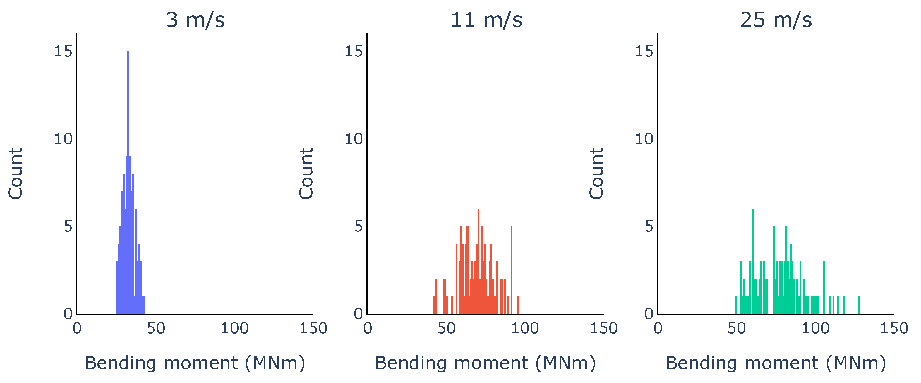
• Combinations of the hub-height mean wind speed (V) and the turbulence intensity (I), accounting for the entire operational range of the turbine, were initially defined. Twelve wind speeds, from the cut-in (3 m/s) to the cut-out (25 m/s) values, stepped at 2 m/s and 3 turbulence intensities (10%, 20%, and 30%) were used.
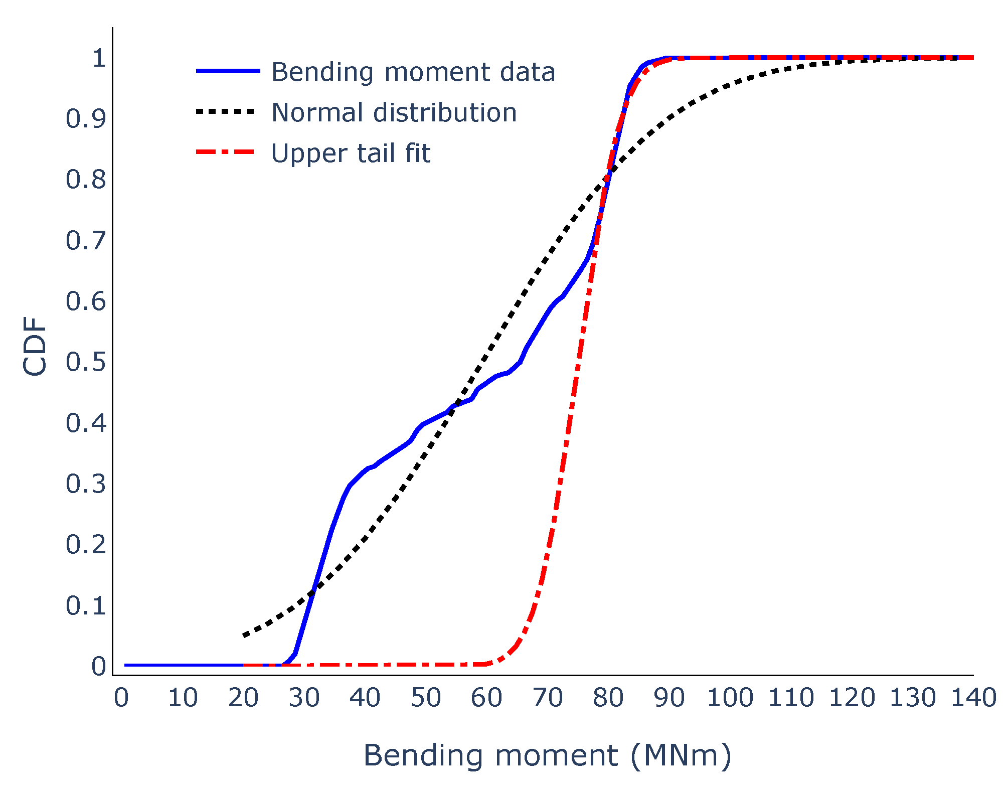
• For each combination of mean wind speed and turbulence intensity, 100 stochastic simulations were carried out using the same set of wind seeds for a total of 3600 simulations. The extreme response after the electrical fault was sampled. For each combination of wind speed and turbulence, a normal distribution was fitted to the extreme responses.
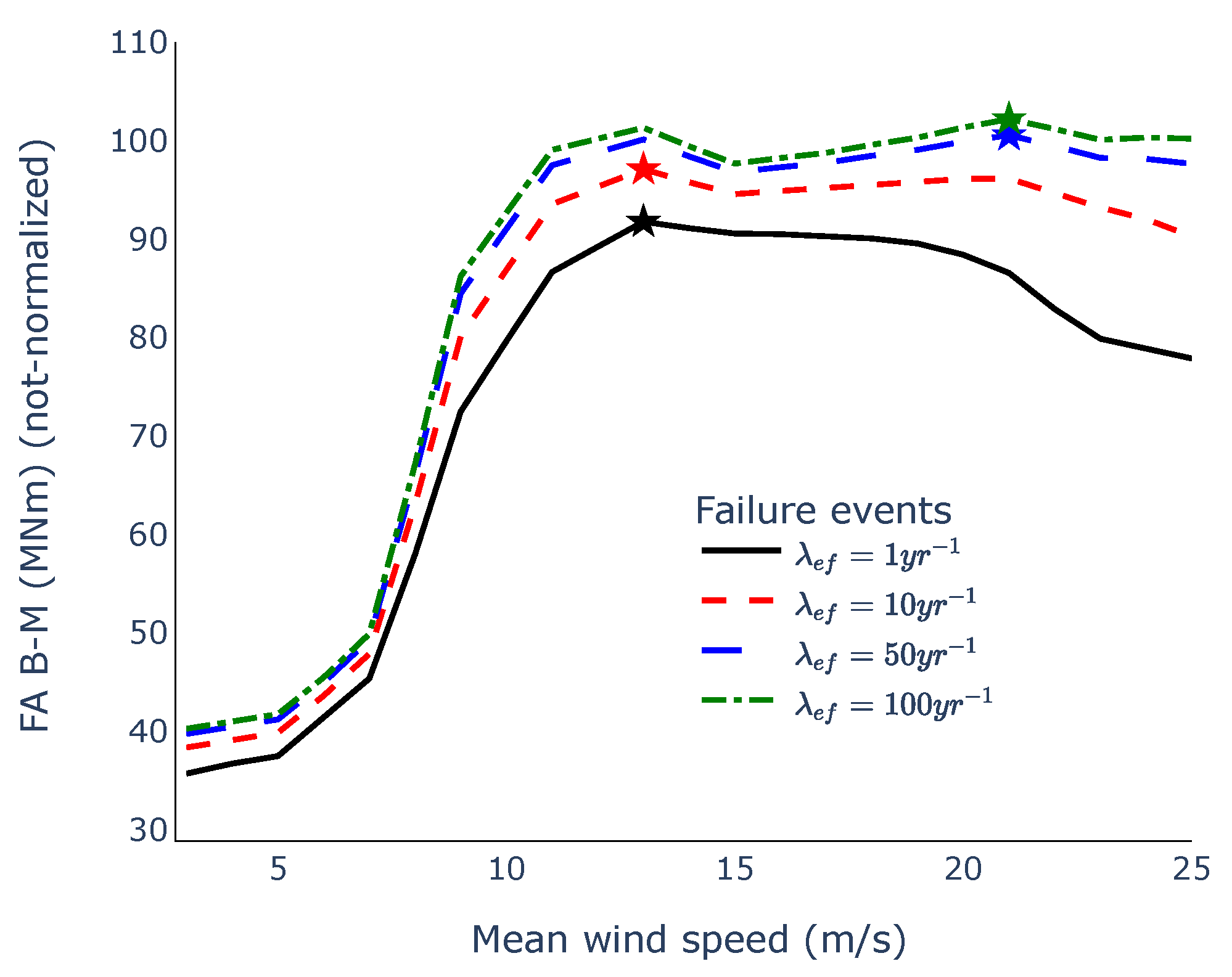
• iFORM was applied for different failure rates.

Figure 7 shows histograms of the obtained responses at three different wind speeds (cut-in—3 m/s, near-rated—11 m/s, and cut-out—25 m/s) for a turbulence intensity = 30%. For each wind speed, 100 simulations were used, although IEC 61400-1 generally only requires 12 simulations for each combination.

The maximum response (fore-aft tower base bending moment) obtained from iFORM for a return period of 50 years is plotted in Figure 8. The curves correspond to different rates of electrical failure: 1, 10, 50, and 100 per year. With an increase in the failure rate, the maximum load from iFORM can be observed to shift to higher wind speeds (from 13 m/s to 21 m/s).

3.1.4. Summary of Section Moduli

The section moduli of the tower base, obtained using the design Equation (3) for each approach, are given in

Table 1. Section modulus of the tower base.

Method	Failure/year	Value (m3)
NREL		0.7532
EOG		0.6340
NTM		0.4661
iFORM	1	0.4187
	10	0.4430
	50	0.4587
	100	0.4662

. The as-designed value from the definition of the NREL 5 MW land-based wind turbine is also shown, which was calculated from a diameter of 6 m and thickness of 0.027 m [27]. The section modulus obtained using the different methods all resulted in values that are smaller than the NREL values. This implies that other load cases or failure modes are driving the design. Of the existing methods in IEC 61400-1, the NTM method resulted in the lowest section modulus. It was seen that almost the same section modulus was obtained using iFORM with a failure rate of 100 per year as for the NTM approach, whereas lower values were obtained for lower failure rates. Assuming that a reduction in the section modulus is obtained by reducing the tower thickness without changing the tower diameter, there is approximately a linear relationship between steel usage and section modulus. It was seen that for annual rates of electrical faults between 1 and 10, a reduction in steel usage of 5–10% was estimated. In the following, the reliability was estimated for the section moduli in Table 1 to assess the reliability resulting from the use of the different design approaches in DLC 2.3.

3.2. Reliability Analysis

First-order reliability method (FORM) [35] was used for the reliability analysis. FORM computations were performed using Python Structural Reliability Analysis (PYSTRA) [36], a Python-based framework for structural reliability analysis. The baseline stochastic variables for the limit state equation (Equation (13)) are listed in

Table 2. Assumptions for limit state equation.

Var.	Distribution	Mean	Std.
$\delta$	Lognormal	1.00	0.05
$f_y$	Lognormal	386 MPa	19.3 MPa
$X_{Str}$	Lognormal	1.00	0.05
$X_{Site}$	Lognormal	1.00	0.10
$X_{Aero}$	Lognormal	1.00	0.10
$X_{Dyn}$	Lognormal	1.00	0.05
$X_{Mat}$	Lognormal	1.00	0.05
$X_{Wind}$	Lognormal	1.00	0.10
$X_{Sim}$	Lognormal	1.00	0.05

[14]. For steel yield stress $f_y$, the mean and standard deviation were calculated assuming a 5% quantile equal to 355 MPa and a COV = 0.05 [37]. The remaining variables in the table are dimensionless model uncertainties with unit mean values. The sectional modulus W was as a deterministic variable with values as given in Table 1, and the modeling of the moment M is given in Section 2.2.

For the tower base bending moment, the modeling depends on the reliability analysis approach. In approach B, the reliability analyses were performed by modeling the load for each combination of wind speed and turbulence intensity by a normal distribution, as described in Section 3.1.3. In approaches A and C, a distribution aggregated over the environmental conditions was used. This was achieved by aggregating the relative frequency diagrams of extreme loads using Equation (16). For the reliability analysis, it was most practical to formulate the load distribution as a continuous distribution, and the fit in the upper tail region was most important. In Figure 9, the empirical distribution of the data is shown, together with a normal distribution fitted to all data and a normal distribution fitted to the upper tail of the distribution using the least squares method. The latter was found to give a good fit in the upper tail, and, as the fit in the remaining part was not important for the reliability analysis results, this distribution was used. The mean and standard deviation values were obtained as 75,000 kN and 5535 kN, respectively.

Results

The annual reliability index was evaluated using all combinations of design approaches (EOG, NTM, iFORM), rate of electrical failure events ${\lambda }_E$ (1, 10, 50, 100), and reliability analysis approaches (A, B, C). The results are given in

Table 3. Reliability indices—approach A.

Failure/year →	1	10	50	100
Method ↓
EOG	5.37	4.94	4.62	4.47
NTM	3.98	3.40	2.93	2.70
iFORM	3.50	3.14	2.84	2.72

,

Table 4. Reliability indices—approach B.

Failure/yr →	1	10	50	100
Method ↓
EOG	5.38	4.96	4.63	4.48
NTM	4.02	3.44	2.98	2.76
iFORM	3.55	3.19	2.89	2.76

and

Table 5. Reliability indices—approach C.

Failure/yr →	1	10	50	100
Method ↓
EOG	5.39	5.07	4.89	4.83
NTM	4.02	3.65	3.46	3.39
iFORM	3.55	3.41	3.38	3.38

and are shown in Figure 10.

Approaches A and B generally gave close to identical results, with differences in the reliability index ranging from 0.01 to 0.06. This confirms that the reliability obtained with the use of the aggregated distribution is almost identical to the reliability obtained when reliability analyses are performed for the individual distributions, as expected. Approach C gives higher reliabilities than A and B for higher failure rates because the correlation between the events is properly accounted for.

The design approaches in IEC 61400-1 (EOG and NTM) do not account for the failure rate in the design; thus, the reliability decreases with increasing failure rate because it is taken into account in the reliability analysis. Since EOG results in a larger section modulus than NTM, it also results in a larger reliability. Using the most accurate approach C, both methods result in reliabilties above the target reliability 3.3, even for failure rates equal to 100.

For iFORM, the failure rate is considered in the design; thus, the section modulus is lower than that of EOG and NTM for smaller failure rates and increases with the failure rate. When reliability approach C is used for assessment, iFORM results in a stable reliability index with a value around 3.4.

4. Conclusions

This work aimed to make recommendations for the use of probabilistic design approaches for DLC 2.3. In addition to the methods included in IEC 61400-1, a semiprobabilistic method based on iFORM was presented. Furthermore, three probabilistic approaches were presented for DLC 2.3, including a novel approach based on the Poisson process. All methods were applies to the NREL 5 MW onshore wind turbine, yielding failure in the tower bottom section due to fore-aft moment. The same approach can be used for other components and failure modes, but additional investigations are needed to assess the inherent reliability of using iFORM for these and to assess the possible reductions in steel usage.

For the failure mode considered in this work, the direct use of iFORM for DLC 2.3 leads to reductions in the design load compared to the methods in IEC 61400-1. If DLC 2.3 is driving the design, the reductions in load could be translated into reduced steel usage and therefore reductions in cost. Compared to designing with the existing approaches in IEC 61400-1, steel reduction of 5–10% could be obtained using the iFORM approach for annual rates of electrical failure of between 1 and 10. The iFORM approach constitutes the background of the existing NTM approach, where a factor of three is used on the standard deviation of the response as a conservative value that is valid for all components and failure rates. The direct use of iFORM is therefore more accurate, as it corresponds to deriving the factor for the specific application.

In reliability approaches A and B, the failure probability is essentially obtained by multiplying the rate of electrical faults by the probability of structural failure given an electrical fault event at a random point in time. For rates of electrical faults larger than one, this is a crude approximation because the limit states for the failure events are correlated, as the exposed structure is the same. Therefore, for higher failure rates, the use of the simple reliability approaches A and B leads to overly conservative results. Approach C leads to more accurate predictions due to the modeling based on the Poisson process, which means that the resistance is assumed to be fully correlated for the electrical fault events affecting the same structure.

When assessing the reliability level using the most accurate method (approach C), the reliability level is consistently above the target for the existing approaches and the iFORM approach. This confirms that the use of iFORM leads to sufficiently reliable designs, while enabling cost reductions. Furthermore, by the use of direct probabilistic design, the tower thickness could be further reduced to just reach the target, thus enabling further cost reductions.

The iFORM and reliability analysis approaches require additional simulations compared to the existing approaches in the standard. However, if DLC 2.3 drives the design, the cost reductions justify this effort. A barrier to the use of probabilistic design methods is the potential difficulties in discussions with certifiers. However, here, the development of IEC TS 61400-9 is an important enabler, and the widespread industrial participation in the work on the technical specification demonstrates the industrial interest in probabilistic design approaches. As an alternative to the direct use of iFORM or probabilistic design, an option is to calibrate specific safety factors for the load case for specific failure modes and fault rates. Although the present work focused on DLC 2.3, the same reliability analysis approaches can be used for other load cases with events such as faults and start-ups/shut-downs.

References

1. GWEC. Global Wind Report—2022; Global Wind Energy Council: Lisbon, Portugal, 2022. [Google Scholar]
2. Stehly, T.; Duffy, P. 2020 Cost of Wind Energy Review; Technical Report NREL/TP-5000-81209; National Renewable Energy Laboratory: Golden, CO, USA, 2022. [Google Scholar]
3. IEC 61400-1:2019; Wind Energy Generation Systems—Part 1: Design Requirements. International Electrotechnical Commission: Geneva, Switzerland, 2019.
4. Sørensen, J.D.; Frandsen, S.; Tarp-Johansen, N.J. Effective turbulence models and fatigue reliability in wind farms. Probabilistic Eng. Mech. 2008, 23, 531–538. [Google Scholar] [CrossRef]
5. IEC 61400-3-1:2019; Wind Energy Generation Systems—Part 3-1: Design Requirements for Fixed Offshore Wind Turbines. International Electrotechnical Commission: Geneva, Switzerland, 2019.
6. Freudenreich, K.; Argyriadis, K. Wind Turbine Load Level Based on Extrapolation and Simplified Methods. Wind. Energy 2008, 11, 589–600. [Google Scholar] [CrossRef]
7. Sørensen, J.D.; Toft, H.S. Safety Factors—IEC 61400-1 ed. 4 Background Document; Technical Report; DTU Wind Energy-E-Report-0066(EN); Technical University of Denmark: Kongens Lyngby, Denmark, 2014. [Google Scholar]
8. Sørensen, J.D.; Toft, H.S. Probabilistic design of wind turbines. Energies 2010, 3, 241–257. [Google Scholar] [CrossRef]
9. Mendoza, J.; Nielsen, J.S.; Sørensen, J.D.; Köhler, J. Structural reliability analysis of offshore jackets for system-level fatigue design. Struct. Saf. 2022, 97, 102220. [Google Scholar] [CrossRef]
10. Deviprasad, B.S.; Chatterjee, S. Reliability analysis of monopiles for offshore wind turbines under lateral loading. Ocean. Eng. 2024, 294, 116829. [Google Scholar] [CrossRef]
11. Nielsen, J.S.; Miller-Branovacki, L.; Carriveau, R. Probabilistic and risk-informed life extension assessment of wind turbine structural components. Energies 2021, 14, 821. [Google Scholar] [CrossRef]
12. Jiang, Z.; Hu, W.; Dong, W.; Gao, Z.; Ren, Z. Structural reliability analysis of wind turbines: A review. Energies 2017, 10, 2099. [Google Scholar] [CrossRef]
13. Nielsen, J.S.; Toft, H.S.; Violato, G.O. Risk-Based Assessment of the Reliability Level for Extreme Limit States in IEC 61400-1. Energies 2023, 16, 1885. [Google Scholar] [CrossRef]
14. IEC CD TS 61400-9; Wind Energy Generation Systems—Part 9: Probabilistic Design Measures for Wind Turbines. International Electrotechnical Commission: Geneva, Switzerland, 2023.
15. Hannesdóttir, Á.; Kelly, M. Detection and characterization of extreme wind speed ramps. Wind. Energy Sci. 2019, 4, 385–396. [Google Scholar] [CrossRef]
16. Hannesdóttir, Á.; Verelst, D.R.; Urbán, A.M. Extreme coherent gusts with direction change-probabilistic model, yaw control, and wind turbine loads. Wind. Energy Sci. 2023, 8, 231–245. [Google Scholar] [CrossRef]
17. Bierbooms, W. Modelling of Gusts for the Determination of Extreme Loads of Pitch Regulated Wind Turbines. Wind. Eng. 2004, 28, 291–303. [Google Scholar] [CrossRef]
18. Bierbooms, W. Specific gust shapes leading to extreme response of pitch-regulated wind turbines. J. Physics Conf. Ser. 2007, 75, 012058. [Google Scholar] [CrossRef]
19. IEC 61400-1:2005; Wind Turbines—Part 1: Design Requirements. International Electrotechnical Commission: Geneva, Switzerland, 2005.
20. Thesbjerg, L. Background for EOG in IEC 61400-1 Edition 3. Private communication.
21. Zhang, X.; Dimitrov, N.K.; Nielsen, J.S.; Abeendranath, A.K.; Sørensen, J.D. Probwind D10: Pre-Standard for Probabilistic Design and Background Document; Technical Report; Aalborg University: Aalborg, Denmark, 2023. [Google Scholar]
22. Tarp-Johansen, N.J. Electrical failure combined with EOG (DLC 2.3). In Proceedings of the MT01 Maintenance Cycle Meeting, Skærbæk, Denmark, 11–12 January 2007. DONG Energy. [Google Scholar]
23. Winterstein, S.R.; Ude, T.C.; Cornell, C.A.; Bjerager, P.; Haver, S. Environmental parameters for extreme response: Inverse FORM with omission factors. In Proceedings of the ICOSSAR-93, Innsbruck, Austria, 9–13 August 1993; pp. 551–557. [Google Scholar]
24. Fitzwater, L.M.; Cornell, C.A.; Veers, P.S. Using environmental contours to predict extreme events on wind turbines. In Proceedings of the Wind Energy Symposium, Madrid, Spain, 16–19 June 2003; Volume 75944, pp. 244–258. [Google Scholar]
25. Dimitrov, N. Inverse Directional Simulation: An environmental contour method providing an exact return period. J. Physics Conf. Ser. 2023, 1618, 062048. [Google Scholar] [CrossRef]
26. Saranyasoontorn, K.; Manuel, L. Efficient models for wind turbine extreme loads using inverse reliability. J. Wind. Eng. Ind. Aerodyn. 2004, 92, 789–804. [Google Scholar] [CrossRef]
27. Jonkman, J.M.; Butterfield, S.; Musial, W.; Scott, G. Definition of a 5-MW Reference Wind Turbine for Offshore System Development; Technical Report NREL/TP-500-38060; National Renewable Energy Laboratory: Golden, CO, USA, 2009. [Google Scholar]
28. Manwell, J.F.; McGowan, J.G.; Rogers, A.L. Wind Energy Explained: Theory, Design and Application; John Wiley & Sons: Hoboken, NJ, USA, 2010. [Google Scholar]
29. DNV-ST-0437; Loads and Site Conditions for Wind Turbines. DNV: Oslo, Norway, 2021.
30. Rosenblatt, M. Remarks on a multivariate transformation. Ann. Math. Stat. 1952, 23, 470–472. [Google Scholar] [CrossRef]
31. Ditlevsen, O.; Madsen, H.O. Structural Reliability Methods; Wiley: New York, NY, USA, 1996. [Google Scholar]
32. Jonkman, J.M.; Buhl, M.L., Jr. FAST – User’s Guide; Technical Report NREL/EL-500-38230; National Renewable Energy Laboratory: Golden, CO, USA, 2005. [Google Scholar]
33. Buhl, M.; Jonkman, J. IECWind—A Utility to Create Wind Files for InflowWind-Based Programs. 2007. Available online: https://www.nrel.gov/wind/nwtc/iecwind.html (accessed on 10 January 2023).
34. Jonkman, B.J. TurbSim User’s Guide: Version 1.50; Technical Report NREL/TP-500-46198; National Renewable Energy Laboratory: Golden, CO, USA, 2009. [Google Scholar]
35. Madsen, H.O.; Krenk, S.; Lind, N.C. Methods of Structural Safety; Dover Publications: Mineola, NY, USA, 2006. [Google Scholar]
36. Hackl, J.; Caprani, C. Pystra—Python Structural Reliability Analysis. 2022. Available online: https://pystra.github.io/pystra/index.html (accessed on 10 May 2023).
37. EN 1993-1-1:2022; Eurocode 3: Design of Steel Structures—Part 1-1: General Rules and Rules for Buildings. European Committee for Standardization (CEN): Brussels, Belgium, 2022.
Figure 1. A typical EOG profile.
Energies 17 01518 g001
Figure 2. Comparison of response for NTM analysis with and without grid loss.
Energies 17 01518 g002
Figure 3. Circle in e u space.
Energies 17 01518 g003
Figure 4. Modeling DLC 2.3.
Energies 17 01518 g004
Figure 5. Tower base bending moment under EOG and fault conditions.
Energies 17 01518 g005
Figure 6. Characteristic load from NTM analysis.
Energies 17 01518 g006
Figure 7. Histogram of tower base bending moments for TI = 30%.
Energies 17 01518 g007
Figure 8. Maximum load from iFORM. The stars highlight the largest values.
Energies 17 01518 g008
Figure 9. Distribution fit for weighted bending moment.
Energies 17 01518 g009
Figure 10. Reliability indices from different approaches.
Energies 17 01518 g010