Article

Wind Turbine Damage Equivalent Load Assessment Using Gaussian Process Regression Combining Measurement and Synthetic Data

Department of Mechanical Engineering, Institute for Integrated Energy Systems, University of Victoria, Victoria, BC V8P 5C2, Canada
*
Author to whom correspondence should be addressed.
Energies 2024, 17(2), 346; https://doi.org/10.3390/en17020346
Submission received: 28 November 2023 / Revised: 2 January 2024 / Accepted: 5 January 2024 / Published: 10 January 2024
(This article belongs to the Special Issue Probabilistic Design and Assessment of Wind Turbine Structures)

Abstract

:
Assessing the structural health of operational wind turbines is crucial, given their exposure to harsh environments and the resultant impact on longevity and performance. However, this is hindered by the lack of data in commercial machines and accurate models based on manufacturers’ proprietary design data. To overcome these challenges, this study focuses on using Gaussian Process Regression (GPR) to evaluate the loads in wind turbines using a hybrid approach. The methodology involves constructing a hybrid database of aero-servo-elastic simulations, integrating publicly available wind turbine models, tools and Supervisory Control and Data Acquisition (SCADA) measurement data. Then, constructing GPR models with hybrid data, the prediction is validated against the hybrid and SCADA measurements. The results, derived from a year of SCADA data, demonstrate the GPR model’s effectiveness in interpreting and predicting turbine performance metrics. The findings of this study underscore the potential of GPR for the health and reliability assessment and management of wind turbine systems.

1. Introduction

Wind turbines operate in harsh environments subjected to intense cyclic high- and low-frequency forces that can compromise their longevity and overall performance. Assessing the fatigue of these structures is crucial for ensuring their optimal operation and maintenance scheduling, determining their remaining useful lifetime, and considering potential lifetime extensions within the wind farm [1,2]. The assessment of fatigue damage accumulation in all components, based on measurements using sensors on a wind turbine, offers a solution. However, this approach requires a large array of sensors, leading to both logistical and financial constraints that are typically not employed on commercial machines [3,4,5]. The use of aero-servo-elastic simulators has been proposed as an alternative solution. These simulators can generate vast amounts of data, which engineers and researchers can subsequently analyze to assess the fatigue life of wind turbines. However, while these simulations provide valuable insights, it is essential to recognize that they often do not align completely with a turbine’s actual environmental conditions and specific as-built characteristics. Thus, while simulators are a valuable tool, their results should be interpreted cautiously and supplemented with real-world data wherever possible to ensure accurate fatigue life assessments. Modern large wind turbines are equipped with Supervisory Control and Data Acquisition (SCADA) [6]. SCADA systems typically collect over 200 variables, often recording and storing as 5- or 10-min averages along with basic statistics such as minimum (min), maximum (max), and standard deviation (STD) for each interval [7]. However, SCADA has reliability and accuracy issues and typically does not include any data field directly related to loads [8]. When load measurements are available from the SCADA system, they cannot be used directly for calculating the fatigue load. This is because the 10-min time scale is insufficient to capture a wind turbine’s dynamic behavior, which mainly requires high-resolution time series. Given all these factors and considerations, one potential solution is to use the SCADA environmental measurements as input for an aero-servo-elastic simulator to compute structural loads, in the absence of physical, e.g., strain gauge measurements. The output can then be utilized to construct a data-driven model capable of estimating and indicating Damage Equivalent Load (DEL) on turbine components.
The load assessment of a wind turbine is a complex task, whether it be in the design phase for a machine, layout optimization of a wind farm, or backing out from operational data. Therefore, many attempts have been made to simplify this task in the literature [9,10,11,12,13]. Dimitrov et al. discussed five different methods, including Kriging and Polynomial Chaos Expansion (PCE), for load assessment using synthetic data [14]. Their results indicate that the mean wind speed and turbulence intensity have the most significant effect on fatigue load estimation. In another study, Haghi and Crawford developed a PCE to map the random phases of synthetic wind to the loads on a wind turbine rotor [15]. Most of the studies in the literature focus on the realm of Surrogate Model (SM)s, attempting to map wind speed by itself or combined with other relative variables to the fatigue or extreme loads of a wind turbine. In recent years, with the rapid growth of Machine Learning (ML) methods, there has been a shift towards using these methods for load assessment. Dimitrov et al. developed an Artificial Neural Network (ANN) to map different environmental conditions to the DEL on a turbine [14]. Schröder et al. used ANN to develop a surrogate model capable of predicting the fatigue life of a wind turbine in a wind farm, considering changes in loads [16]. More recently, Dimitrov and Göçmen developed a virtual sensor based on a sequential ML method that can provide load time series for different components of a wind turbine [17].
Condition Monitoring (CM) for wind turbines is an activity that monitors the state of the turbine [18]. CM is vital for wind turbines as it can reduce downtime, failure, and maintenance costs. There are various techniques available for the CM of wind turbines; however, many are either expensive or complex [3,8]. Consequently, utilizing data from SCADA for CM is appealing, as these data are available for the majority of turbines and do not incur additional costs [19]. Tautz-Weinert and Watson provide an extensive review of the different CM methods that utilize data from SCADA. A few of these methods address damage modeling and fatigue of components. The concept behind damage modeling is to integrate measurements from SCADA with a physical model to understand better damage progression [8]. Gray and Watson introduced a probability of failure methodology incorporating relatively simple failure models and successfully tested this method on a wind farm with a high rate of gearbox failure [20]. Galinos et al. created a map of the fatigue life distribution for the Horns Rev 1 offshore wind farm turbines using SCADA wind speed measurements and aeroelastic simulations [21]. Alvarez and Ribaric used SCADA to describe the wind turbine torque histogram and introduced a methodology for a physics-based gearbox fatigue failure prediction [22]. Remigius and Natarajan utilized SCADA measurements to estimate the wind turbine main shaft using an inverse problem-based approach [23]. The examples mentioned above are mainly based on a physics-driven approach.
In recent years, with the emergence of data-driven methods, the integration of SCADA measurements with ML-based methods has become more popular among researchers. Pandit et al. provided an extensive review of data-driven CM approaches [24]. More specifically, data-driven methods using SCADA measurements have been increasingly adopted for predicting fatigue life and damage. Vera-Tudela and Kühn employed ANN to map wind farm varying flow conditions to fatigue loads and demonstrated the robustness of this method by using data from two distinct wind farms [25]. Natarajan and Bergami found that an ANN could predict turbulence and loads on the blade and tower by considering rotor speed, power production, and blade pitch angle from SCADA measurements, validating the loads using an instrumented turbine [26]. Mylonas et al. developed a regenerative model based on a convolutional variational autoencoder, capable of predicting DEL on a wind turbine blade root and the uncertainty of loads using only 10-min average SCADA data [27].
A Gaussian Process (GP) is a type of ML technique used for both regression and classification problems. It is a data-driven, non-parametric method that does not rely on a specific functional form. Instead, it focuses on a distribution of functions that align with the data it is analyzing [28]. The application of GP in wind turbine research and engineering has grown due to the ease of implementation, versatility, and adaptability of the method, as well as its ability to provide uncertainty estimates. For instance, Pandit and Infield utilized GPR to capture failures due to yaw misalignment using SCADA [29]. Li et al. employed Gaussian Process Classification (GPC) to detect and predict wind turbine faults from SCADA data, where the provided probabilistic knowledge aids in maintenance management [30]. Herp et al. utilized GP to forecast wind turbine bearing failure a month in advance based on wind turbine bearing temperature residuals [31]. Avendaño-Valencia et al. predicted wind turbine loads in downstream wakes, calibrating a GPR based on local or remote wind or load measurements [32]. Wilkie and Galasso assessed the fatigue calculation reliability of offshore wind turbines using a GPR, where inputs consisted of site-specific environmental conditions and turbine structural dynamics [33]. Singh et al. employed chained GP to derive the probability distribution function of offshore wind turbine loads based on stochastic synthetic loads [34].

1.1. Motivation

In this manuscript, we aim to create a simple yet dependable probabilistic model for predicting damage using limited SCADA measurements and utilizing publicly available wind turbine models. The inflow turbulence is stochastic, leading to load responses that are aptly represented as random variables. The influence of these unpredictable factors on loads heavily depends on average environmental conditions and their variance. This variance in load response, known as heteroscedasticity in statistical terms, implies that at lower wind speeds, the inflow turbulence has a lesser impact on load variability compared to higher wind speeds [34]. Heteroscedasticity directly affects the DEL of a wind turbine. The challenge is that to obtain an accurate distribution of the DELs for an operational turbine, we require many data points. Ideally, this could be achieved with an extensive array of sensors on wind turbines, which is not feasible. One approach involves running simulations to enrich the database and attain improved distributions. However, two primary challenges exist: (a) the models lack accuracy, and (b) wind turbine manufacturing companies view models as their intellectual property, making them generally inaccessible.
Given these challenges, our proposal is not for a highly accurate model to predict the DEL down to the minutest details. Instead, we advocate for a straightforward methodology to offer a probabilistic model built on hybrid SCADA and publicly available turbine models. This model can approximate the DEL distribution at each wind speed and demonstrate the trend of the DEL distribution as wind speed varies. Although this model might not be precise enough to indicate the remaining useful lifetime with high accuracy, it can roughly gauge the turbine fatigue health condition and relative damage of machines within a wind farm. Such a model can serve as a quick indicator to pinpoint turbines at risk, warranting further investigation. Additionally, it can assist in reducing the uncertainty of a turbine’s health condition for financial and banking purposes. This model demonstrates benefits for “asset reliability” and “asset health”, especially in mitigating investor risks when considering the purchase of operational wind farms.

1.2. Objective

For this research, we had access to a year’s worth of data from an undisclosed turbine in an undisclosed onshore wind farm’s SCADA system. The objectives of this manuscript are as follows:
  • Create a database of synthetic DEL based on publicly available turbine models with SCADA wind measurements as input.
  • Develop a probabilistic model based on the database that represents the distribution of the descriptive statistics and DEL at varying wind speeds.
  • Validate the probabilistic model by contrasting its output with the limited available measurements.

1.3. Paper Outline

The paper is organized as follows: Section 2 starts with an overview of the methodology, depicted in Figure 1, and continues with a description of the SCADA system used in the study, including data collection and processing methods. This is followed by an explanation of joint distributions and sampling in Section 2.2, and the basics of aero-servo-elastic simulations and their post-processing. Section 2.5 introduces the Gaussian Process Regression (GPR) methodology applied in this study and concludes Section 2 with a definition of the error metrics used. Section 3 begins with the conditions under which results are extracted and GPR models are trained, continuing with the validation of these models against empirical data. The accuracy of the trained GPR, using hybrid data, is compared with both simulations and SCADA data in Section 3.1 and Section 3.6. Section 3 ends with proposed practical applications for the developed model. The manuscript concludes with Section 4, summarizing the main findings and suggesting future research in using GPRs for wind turbine primary health assessment.

2. Methods

This section presents the methodology used to construct a GPR model using hybrid simulation and validate the GPR predictions against both hybrid simulation and SCADA measurements. Figure 1 provides an overview of our approach, consisting of four blocks. The arrows illustrate the data flow between these blocks, databases, and processes. Hereafter, “wind speed” refers to the measured wind speed from SCADA, unless otherwise specified. It is worth mentioning that the wind speed sensor on a wind turbine is typically placed on top of the nacelle behind the rotor, and its readings differ from the true inflow wind speed.
The hybrid simulations generation block demonstrates the procedure for generating hybrid simulation data from SCADA measurements. Termed “hybrid”, this data combines SCADA measurements with synthetic data generation to create a comprehensive database. The SCADA data is binned to a resolution of 1 m/s, spanning the cut-in and cut-out wind speeds. The turbine in this study operates between 3 m/s and 25 m/s. For each bin, we establish a joint distribution of mean wind speed and STD of wind speed. The mean wind speed adheres to a uniform distribution between the bin’s upper and lower bounds, whereas the wind speed STD distribution sampling per bin is tested on both Weibull and uniform distributions separately.
Subsequently, using Sobol sampling, n samples are drawn from this joint distribution for each wind speed. Each sample, comprising a mean and STD of wind speed, generates a synthetic wind field. This results in a corresponding synthetic wind field per sample. These synthetic wind fields and the wind turbine model are inputs to the aero-servo-elastic simulator. The simulator outputs load time series for various components of the wind turbine model. These load time series are post-processed to extract statistical descriptions (minimum, maximum, mean, and STD) and the DEL for each component. In this manuscript, the post-processed outputs are termed Quantity of Interest (QoI). The QoI are stored in a database, referred to as the post-processing database.
The Gaussian Process Regression block outlines the technique employed to build the GPR model using hybrid simulation output. The post-processing database is initially scaled using the MinMax method to normalize all data fields between 0 and 1. The database is then divided into two non-overlapping datasets: Training and Testing. A separate GPR model is trained for each QoI for each wind turbine component load. The GPR model outputs the mean and STD of the QoI at each wind speed, representing the prediction data statistics. The testing data similarly provides the mean and STD of the QoI at each wind speed, known as the testing data statistics.
Figure 1 illustrates two validation blocks: Hybrid Validation and SCADA Validation. For Hybrid Validation, the testing data statistics are compared against the prediction data statistics. If the SCADA data include tower top acceleration or blade load statistics, the GPR prediction distribution for these is also validated.
In the following sections, we delve into the processes and steps depicted in Figure 1 in greater detail.

2.1. Supervisory Control and Data Acquisition Measurement, Binning, and Scaling

The comprehensiveness of the collected SCADA data offers a wide range of insights for system analysis. Notably, the SCADA data encompasses numerous data fields, with our primary interest in wind speed statistics for hybrid simulation database generation, generated power for wind turbine model validation, and, if available, tower top acceleration and blade load statistics for measurement validation.
We binned the SCADA data based on mean wind speed to gain a broader perspective on wind turbine operation through the wind speed statistics. The bin center corresponds to an integer wind speed value, with the upper and lower bounds set at ± 0.5 m/s of that value. For each bin, we calculated the mean of the measured mean wind speed, the mean of the STD of the wind speed, and the STD of the STD of the wind speed, resulting in three wind speed statistics for each bin.
MinMax scaling is a common pre-processing step in data analysis and machine learning, involving transforming features to a specified range, often [ 0 ,   1 ]  [35]. According to Rasmussen and Williams, scaling the data is recommended for GPR to ensure numerical stability [28]. For the post-processing database, we scaled the data based on the minimum and maximum values in each wind turbine channel output, effectively constraining each scaled post-processed output to the [ 0 ,   1 ] range. Additionally, if SCADA loads or acceleration measurements were available, they were scaled similarly to facilitate comparison with the GPR output. Furthermore, we adopted MinMax scaling for all output data in compliance with confidentiality requirements.

2.2. Joint Distributions and Sampling

Hybrid simulation data generation aims to build a comprehensive database of the loads on a wind turbine, closely resembling real-world conditions. This process, known as data assimilation [36], merges observational data (in our case, SCADA data) with model predictions to produce a more complete estimate of the current state of the system and future evolution. One approach to account for measurement uncertainties is to define them as random variables with specific distributions. We utilized wind speed statistics extracted in Section 2.1 to construct joint distributions of mean wind speed and the STD of wind speed for each bin. A uniform distribution was defined to cover the full range of the bin for the mean wind speed equally. Regarding the STD, we opted to test two alternatives: (a) fitting a Weibull distribution to the STD of wind speed, and (b) applying a uniform distribution to the STD, with bounds set at the minimum and maximum values per bin. The assumption of a uniform distribution for wind speed has been previously established in literature [14,16]. The choice of a Weibull distribution for the STD is based on data observations, and a uniform distribution is selected to encompass all possibilities, particularly when SCADA measurements in a bin are unavailable.
We employed the Quasi Monte Carlo (QMC) Sobol sampling technique, as detailed in [37]. This method is preferred in our study for its reliability and computational efficiency, as noted in [38]. Sobol’s technique is repeatable and ensures enhanced uniformity across sampled distributions, a feature emphasized in [39]. Hereinafter, “the sample” refers to a two-data-point vector comprising mean wind speed and STD of wind speed. We took n samples per bin, resulting in n unique samples for m bins, which are then used to generate n × m synthetic wind time histories.

2.3. Synthetic Wind Generation, Wind Turbine Models, and Aero-Servo-Elastic Simulations

To perform aero-servo-elastic simulations, we require synthetic wind time histories that closely resemble real-world wind conditions experienced by the turbine. To achieve this, we constructed joint distributions from the SCADA measurements and calculated statistics for each wind speed bin as explained in Section 2.2. The objective was to generate synthetic wind time histories that faithfully replicate the actual wind conditions corresponding to the mean and STD of wind samples. To do so, we used the samples’ wind speed and STD as the input to TurbSim [40]. The output of TurbSim is a “full-field” wind time history in TurbSim format. TurbSim, a synthetic wind generator, produces wind time histories with both spatial and temporal components for aero-servo-elastic simulators. A comprehensive explanation of this synthetic wind generator can be found in [40].
The resulting n × m full-field synthetic wind time series are stored in the synthetic wind database. The full-field synthetic wind data serve as the environmental input for our aero-servo-elastic simulator. These simulations require synthetic wind time series and the integration of aerodynamic, aeroelastic, and controller models. Each wind turbine model encompasses modules for aerodynamics, aeroelasticity, and control. To conduct these simulations, we employed OpenFAST, an aero-servo-elastic solver developed by National Renewable Energy Lab (NREL) [41]. The output from OpenFAST provides detailed load information for various wind turbine components, including blades, towers, and gear systems, spanning both time and space. Our simulations adhere to the IEC standards for energy production under Design Load Case (DLC) 1.2, as specified in the IEC standards [42].
The provided SCADA data correspond to a year’s worth of data, which include loads and acceleration data. However, as the turbine models are the intellectual property of the wind turbine manufacturers, we did not have access to them. Therefore, we opted for the NREL 5MW turbine for the aero-servo-elastic simulations [43] as this model is well established in the literature, demonstrates robustness against fluctuations in wind speed seed during simulations, the controller is well defined, and the rotor size is comparable with the turbine we have access to the SCADA measurements. Moreover, our tests indicate that the NREL 5MW model provides simulation results most similar to SCADA data at hand compared to other publicly available turbines [44,45,46].

2.4. Post-Processing Database

We have compiled a comprehensive database incorporating all time series data from the simulation outputs. Following its creation, the data underwent post-processing to derive simulation QoI, namely, descriptive statistics and DEL for assessing loads and fatigue. Additionally, DEL computation adheres to the Palmgren–Miner linear damage rule, as elaborated in [47,48]. The DEL can be expressed as follows:
D E L = Σ n i R i m n e q 1 / m
Here, m represents the Wöhler slope, while R i and n i pertain to load ranges and the corresponding number of cycles, respectively. The DEL outcome is derived through rainflow counting of the load time series [47,49]. n e q denotes the equivalent number of load cycles, typically equivalent to the length of the simulations in seconds. The post-processing database encompassed all calculated descriptive statistics and DELs from every simulation output.
Subsequently, the post-processing database is subjected to MinMax scaling and binning, which were explained in Section 2.1.

2.5. Gaussian Process Regression

GPR is a non-parametric Bayesian method widely used for regression tasks [28]. At the core of GPR lies its assumption that observed target values follow a multivariate Gaussian distribution. One of its notable features is its ability to provide probabilistic predictions, offering both mean and variance functions to quantify prediction uncertainty. Given a dataset ( x 1 , y 1 ) , , ( x N , y N ) , a Gaussian Process defines a distribution over functions characterized by a mean function m ( x ) and a covariance (kernel) function k ( x , x ) . The GPR can be expressed as:
f ( x ) GPR ( m ( x ) , k ( x , x ) )
where, m ( x ) represents the mean function, and  k ( x , x ) is the covariance function, capturing the data point relationships. Predictions f * at new data points x * are expressed as predictive mean μ * and variance Σ * :
μ * = K * T ( K + σ n 2 I ) 1 y
Σ * = K * * K * T ( K + σ n 2 I ) 1 K *
where K is the covariance matrix for the training data, K * represents the covariance matrix between training and test data, and  K * * is the covariance matrix for the test data. y is the vector of training targets, and  σ n 2 is the noise variance. Typically, noise variance and other hyperparameters of GPR and kernel function parameters are estimated from the data, often using techniques like maximum likelihood estimation. The log-likelihood of observations conditioned on hyperparameters is expressed as:
log p ( y | x , θ ) = 1 2 y T ( K + σ n 2 I ) 1 y 1 2 log | K + σ n 2 I | N 2 log 2 π
where y represents the vector of observed target values, K is the covariance matrix calculated using the kernel function for training inputs, and  σ n 2 denotes the noise variance. | K   +   σ n 2 I | signifies the determinant of the matrix, and N is the dataset size. Maximum likelihood estimation aims to determine the hyperparameters θ that maximize this log-likelihood.
For the problem at hand, the x values are the wind speeds, and the y values are the QoI. Recalling the number of bins m and the number of samples n, we have n × m data points, which can result in a large number of data. Moreover, the target data y is a heteroscedastic variable. In our case, it means the data variance is not constant across wind speeds. Due to these two characteristics of the data at hand, standard GPR formulation is ineffective for our purpose. The standard GPR method implementations require O ( n 3 ) computation, where n is the number of data samples [50]. Furthermore, standard GPR assumes the variance across the data is constant. [51]. To tackle these two, we used Approximate Gaussian Process Regression (AGPR) for the large-size dataset challenge with “inducing points” [50] and Predictive Log Likelihood (PLL) for the heteroscedasticity challenge [52]. AGPR introduces a set of inducing points or pseudo-inputs representing a subset of the training data. The GP is conditioned on these inducing points rather than the entire dataset, reducing computational complexity [50]. The standard likelihood tries to maximize the posterior estimation, while PLL, instead of estimating the posterior, directly aims for the posterior distribution estimation [52]. Both of these methods have been thoroughly explained in various literature. For a deeper understanding of these methods, readers are encouraged to refer to [50,52,53]. In this work, we utilized GPyTorch for building the GPR models [54].

2.6. Measurement Statistics and Error Metrics

If the SCADA measurement data include loads or tower top acceleration information, it offers an opportunity to compare these data points with the AGPR output. Given that the output from AGPR is probabilistic, processing the SCADA measurement data to extract relevant statistics becomes necessary. This procedure mirrors the one detailed in Section 2.1. Initially, we scale the measurements using MinMax scaling. Subsequently, we categorize the scaled SCADA measurement loads and acceleration data based on SCADA wind speed measurements and then calculate the mean and STD of acceleration and loads within each bin.
We assess the disparity between the SCADA measurement and AGPR output, or between the AGPR output and the testing datasets, using Kullback-Leibler (KL) divergence. The KL divergence is formulated as:
D K L ( G | | M ) = 1 2 log σ M 2 σ G 2 + σ G 2 + ( μ G μ M ) 2 σ M 2 1
where, in (6), G represents the AGPR output with mean μ G and variance σ G 2 , and M signifies the measurement or simulation data with mean μ M and variance σ M 2 . This comparison involves computing the KL divergence, with the testing database and SCADA measurement serving as the reference or “ground truth”. In cases where we have samples from both AGPR and SCADA, the KL divergence is formulated as:
D KL ( G M ) = i G ( i ) log G ( i ) M ( i )
where G ( i ) and M ( i ) are the probability distributions at bin i for the two distributions, respectively. The bins are set identically for both distributions. The KL divergence has the minimum value of zero and no upper bound. If the KL divergence is zero, it indicates that the two distributions being compared are identical. Therefore, smaller values are preferable. For a more detailed discussion of this topic, interested readers are referred to Murphy [55].

3. Results and Discussion

In this section, we explain the conditions used for generating the results, followed by the presentation of the results and their corresponding discussions. In this section, whenever we refer to a QoI or a data field, it is scaled using MinMax scaling.

3.1. SCADA Measurement

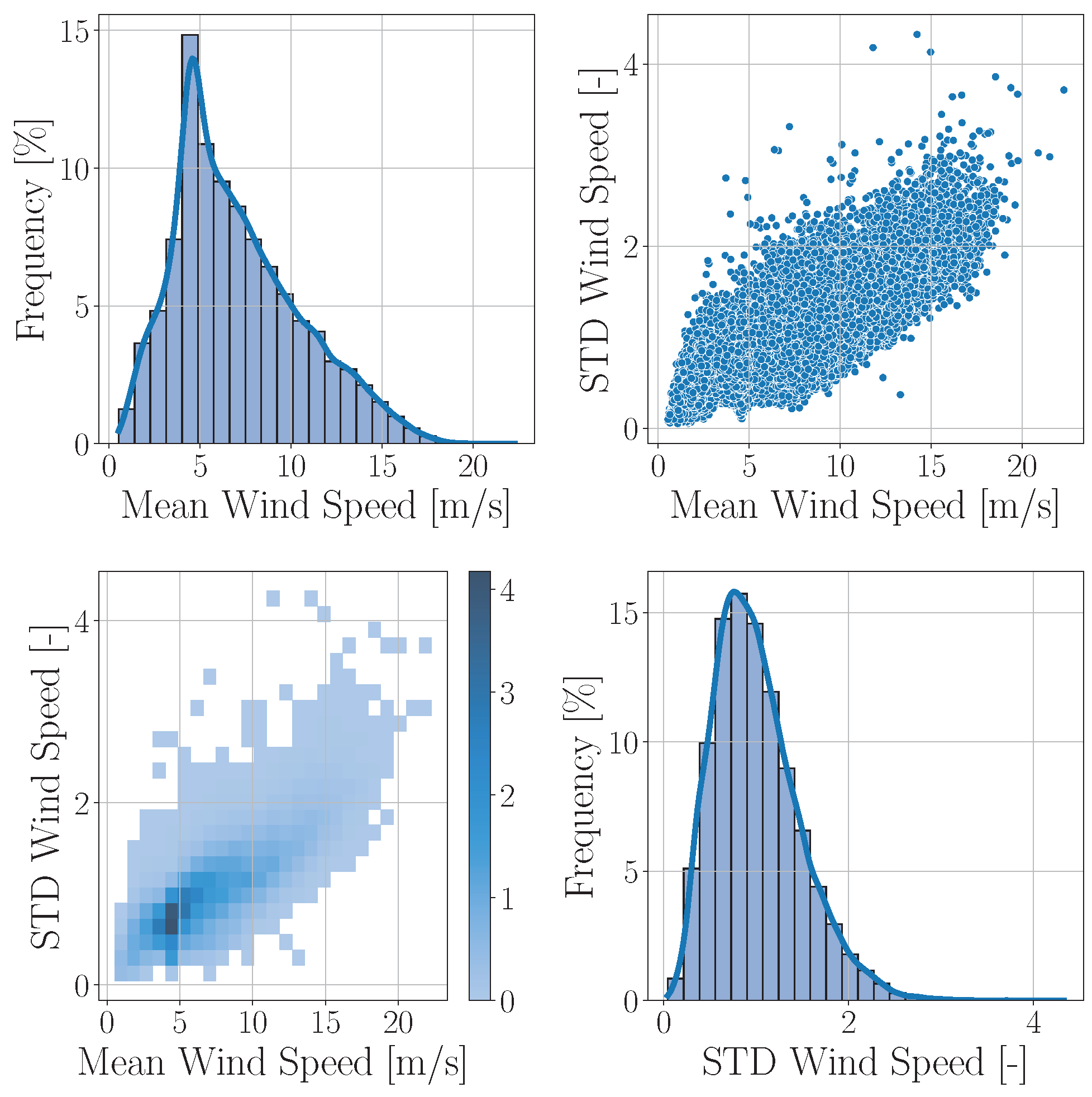
As mentioned, we considered a year’s worth of SCADA measurement data.The SCADA data are filtered only to include data points where the power generated exceeds zero. To understand the environmental conditions in which the turbine operates, the measured mean wind speed and STD wind speed are illustrated in Figure 2.
In Figure 2, the diagonal plots are histograms of the mean wind speed and the STD of wind speed. The off-diagonal plots are scatter plots for the mean and STD on the top right, and the 2D histogram of the mean and STD at the bottom left. This shows that we have reasonable variability in a year to cover different operational conditions.
In addition to wind measurement, the SCADA database contains other data fields. Table 1 provides these additional data fields from the SCADA we utilized in this study and their post-processed data field availability.
We will utilize the data fields in Table 1 in Section 3.5 and Section 3.7 to test the simulation models and the AGPR outputs. We received the measurement data as a 10-min average without access to the underlying time series; therefore, we cannot comment on the noise’s effect or the noise level in the data.

3.2. Joint Distributions and Sampling

As described in Section 2.1, we binned this raw data based on wind speed and processed them to construct joint distributions within each bin. The centers of the bins range from 3 m/s to 25 m/s with a resolution of 1 m/s. The edges of the bins are ± 0.5 m/s from the center of the bins. The edges of the uniform distribution for wind speed coincide with the bin edges. We have two types of joint distributions per bin: Uniform-Weibull (UW) joint distribution for each bin, and Uniform-Uniform (UU) joint distribution per bin. After building the joint distributions, we sampled from these distributions as input to the synthetic wind generator. Each sample contains a mean wind speed and standard deviation.
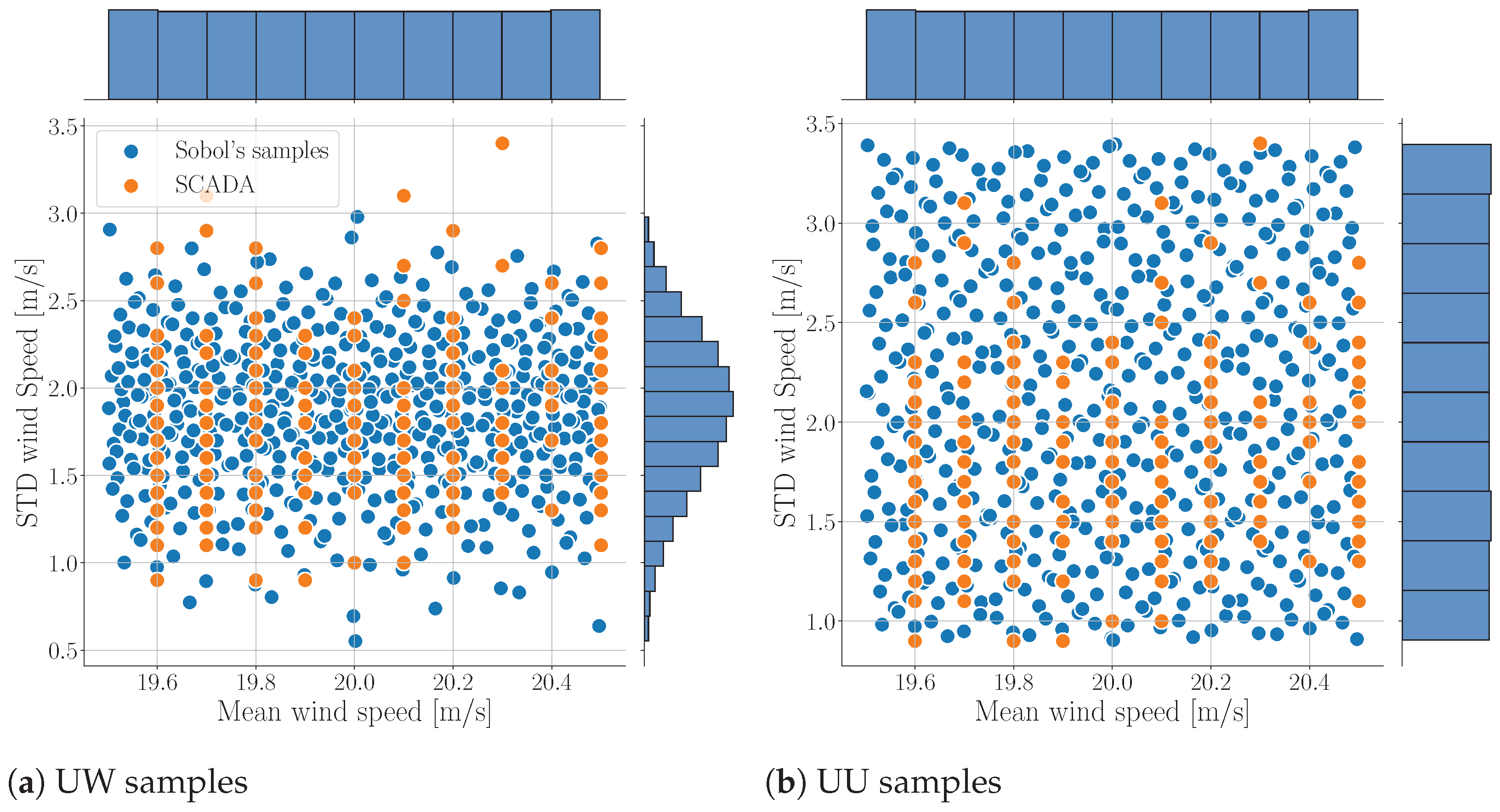
As detailed in Section 2.2, we employed the Sobol sampling technique for our investigation. To maintain the balance characteristics of Sobol sequences, they must be of the form 2 n  [56]. Consequently, we chose 2 9 samples from the set distributions for each bin. We opted for this sample size as the Sobol sampling approach allows us to minimize the sample count without compromising the method’s advantages or needing to resample areas. Additionally, it provides a substantial database for testing purposes. To illustrate, we presented the samples of the 20 m/s bin for both UW and UU in Figure 3. In Figure 3, it appears the provided SCADA for the mean wind speed is rounded to the nearest 0.1 m/s, which is why they are clustered at specific wind speeds. This aspect should be considered when comparing the SCADA with AGPR outputs later in this manuscript.

3.3. TurbSim and OpenFAST Output

The output format of TurbSim is comprehensively detailed in [40]. This output encompasses both spatial and temporal dimensions. Spatially, it provides a synthetic wind time series at various grid locations across the rotor plane. Specifically, TurbSim generates three wind time series corresponding to the x, y, and z directions for each grid point. In our research, we utilized a grid of 15 in the x-axis by 15 in the z-axis over the rotor plane. Temporally, the synthetic wind series operates at a frequency of 20 Hz over a span of 720 s. As previously indicated, we executed aeroelastic simulations on the wind turbine model outlined in Section 2.3 via OpenFAST. OpenFAST provides various outputs, referred to as channels, for different turbine parts. Detailed descriptions of these channels are available in [57].
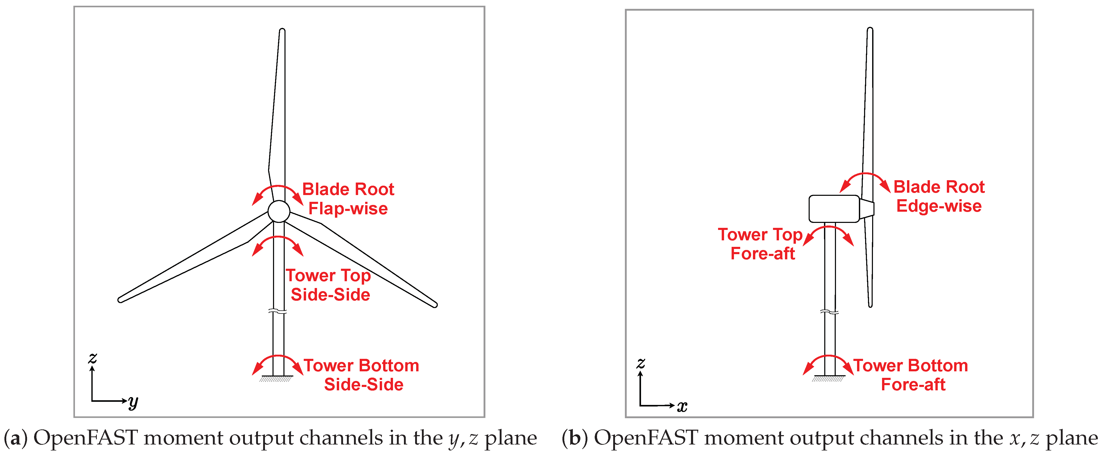
In this study, we evaluated six distinct output channels for DEL along with the mean values for TT side-side, fore-aft, resultant absolute acceleration, rotor speed, and power. These moments encompass blade root (BR) in edge-wise and flap-wise directions, TT in fore-aft and side-side motions, and similarly, tower-base (TB) in fore-aft and side-side movements. The wind turbine load channel positions used in this study are graphically depicted in Figure 4a,b. A comparison between the OpenFAST output channel descriptors and the names we adopted for this research is provided in Table 2.
The out-of-plane BR moment is similar to the edge-wise BR moment in definition, with the primary difference being the coordinate system in which the moment is calculated. OpenFAST calculates the moment in the “blade” coordinate system for the edge-wise moment, while the out-of-plane moment is calculated in the “cone” coordinate system. For a detailed explanation of these coordinate systems, the interested reader is referred to the OpenFAST manual [57]. The TT resultant acceleration, YawBrTAccl, is not directly provided as an OpenFAST output but is computed separately after running the simulations. The resultant acceleration is formulated as follows:
Y a w B r T A c c l ( t ) = Y a w B r T A x p ( t ) 2 + Y a w B r T A y p ( t ) 2
For this analysis, we initiated a total of 2 × 23 × 2 9 = 23,552 aeroelastic simulations via OpenFAST. These simulations were run in 5888 parallel batches, each comprising four simulations, utilizing resources from the Digital Research Alliance of Canada. Each simulation lasted for 720 s, with the initial 120 s omitted to negate the start-up effects. The aeroelastic simulation used a time step of 0.005 s for the simulations, while the output was registered at 20 Hz resolution. Upon completion of all simulations and subsequent database formation, we derived statistical descriptions and DEL for every simulation concerning the channels of interest, adopting a Wöhler slope of m = 4 and n e q = 600 in Equation (1). For simplicity, one Wöhler slope was used for all the load channels, with  n e q equaling the simulation length in seconds [47,48]. The 10-min mean of power generation was also considered. The pyFAST Python library, referenced in [58], was employed to interpret the OpenFAST output files, compute statistical values, and determine the DEL. Through our testing of DEL calculation (10 Hz, 5 Hz, and 1 Hz), we have discovered that altering the sampling frequency of simulation outputs had little impact. Furthermore, the pattern of DEL across different wind speeds remained steady for different sampling frequencies. As all outputs in this study are scaled to be between 0 and 1, the trend of DEL bears greater importance than its numerical values.

3.4. AGPR Training and Testing

For each moment or acceleration channel in Table 2, we developed and trained a AGPR model. The basic background of the AGPR models is explained in Section 2.5. The AGPR models and training settings implemented in GPyTorch are presented in Table 3.
The DEL moments database was divided into two equally sized datasets for training and testing. The training dataset was further divided into 80% for training and 20% for validation of the AGPR model. As the training dataset was large, k-fold cross-validation was not utilized, which is more applicable for smaller databases to prevent overfitting [59]. For the 10-min mean moments and acceleration, we trained the AGPR on the entire simulation outputs dataset with 80% for training and 20% for validation split. Then, we tested the GPR on the SCADA data. How the turbine load for each output channel changes with wind speed depends on the output location. The settings and parameters listed in Table 3 were tuned manually. Different settings were tested for different outputs, and the configurations provided were optimized to achieve similar accuracy across all outputs.

3.5. Wind Turbine Model Verification

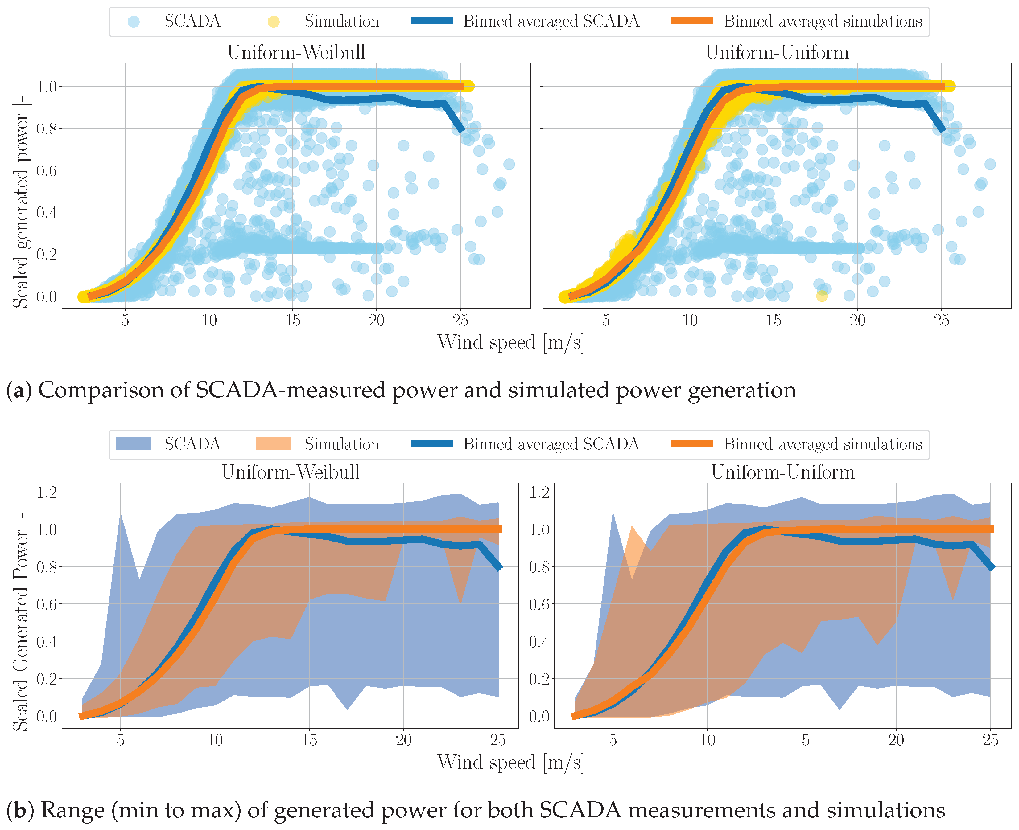
After running the simulations and extracting the QoI to construct the databases, the initial step involved verifying the simulation model’s accuracy against SCADA measurements. Power output and rotor speed were two of the most reliable indicators among the data fields available for measurements and simulations. The trends of these two variables indicate the level of agreement between the wind turbine model and simulations. Additionally, comparing the range of these two outputs for both simulations and SCADA measurements is important. This comparison between SCADA-measured power and the 10-min mean of simulated power for UW and UU is depicted in Figure 5a.
In Figure 5a, the x axis indicates the mean wind speeds of SCADA measurement and simulations. Each data point on the graph is a 10-min mean of generated power, either from SCADA measurements or simulations. Since each simulation duration is 10 min, the displayed value is the mean generated power for that interval. The solid lines on the graph represent the power averaged for each wind speed bin, as explained in Section 2.1. The MinMax scaling is based on the binned average power for both the SCADA measurements and the simulations. There are notable distinctions between Figure 5a,b in terms of their data representation and scaling methodologies. Figure 5a specifically utilizes 10-min average values from both the SCADA system and simulations. These values are normalized using the MinMax scaling approach. In contrast, Figure 5b focuses on the 10-min min and max values obtained from the SCADA system and simulations. The scaling applied here ensures that the mean value of generated power is standardized to one. This distinction in data selection and scaling techniques underscores the different analytical perspectives offered by each figure. It is worth mentioning that values equal to zero in Figure 5a represent the minimum power generation and not zero generated power, as the MinMax scaling output ranges between zero and one.
While the plots demonstrate a good match between simulation and measurements, the measured data exhibits more variability than the simulations, which is expected due to the variability in turbine behavior within 10-min intervals. We computed the difference between the scaled binned averaged measured and simulated power to assess their disparity. The results for a selection of wind speeds are shown in Table 4. The difference in the UU case for 5 m/s is higher than it appears on the plot, as the scaled power values for measurements and simulations are both in the range of 0.01 to 0.02 .
Figure 5b displays the range between the minimum and maximum power from SCADA measurements and simulations. The upper and lower bounds are based on the measurements’ or simulations’ 10-min maximum and minimum values. The shaded area indicates the range for the simulations and SCADA data. As shown in Figure 5b, the range is wider for SCADA measurements than for simulations, which is anticipated.
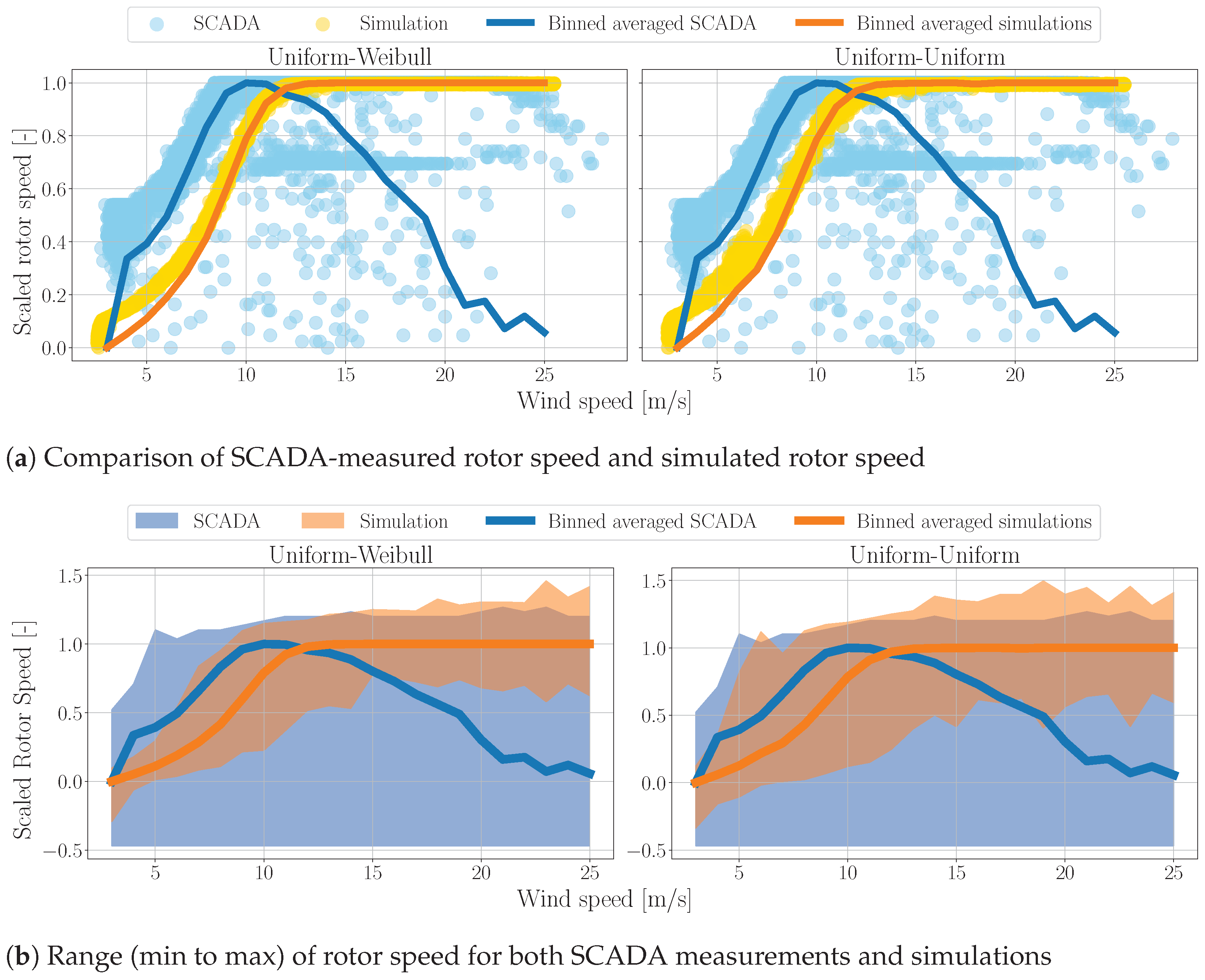
Another indicator for assessing the alignment of the utilized model with real-world turbine behavior is the rotor speed. Similarly, Figure 6a,b compare the 10-min mean and range for the rotor speed. These figures show a notable discrepancy between simulations and SCADA measurements. There are two reasons for this observation: (a) for below-rated wind speeds, the controller behavior of the model and the SCADA-measured turbine differs; (b) for above-rated wind speeds, we lack sufficient measurement data, and the available data are based on unknown parameters that reduce the mean rotor speed. The limited availability of SCADA data and lack of variables such as pitch angle hinder a more accurate understanding of wind turbine behavior. Although there is a discrepancy between the model and SCADA rotor speed, the effect on the purpose is insignificant, as the rotor speed is mainly a function of wind speed and would not affect the SCADA load measurement from the turbine. It is important to note that the aim of this work is not to produce a fully accurate wind turbine simulator, but rather a practical relative health assessment tool when the manufacturer’s turbine model is unavailable.

3.6. AGPR Testing Results—Hybrid Simulations

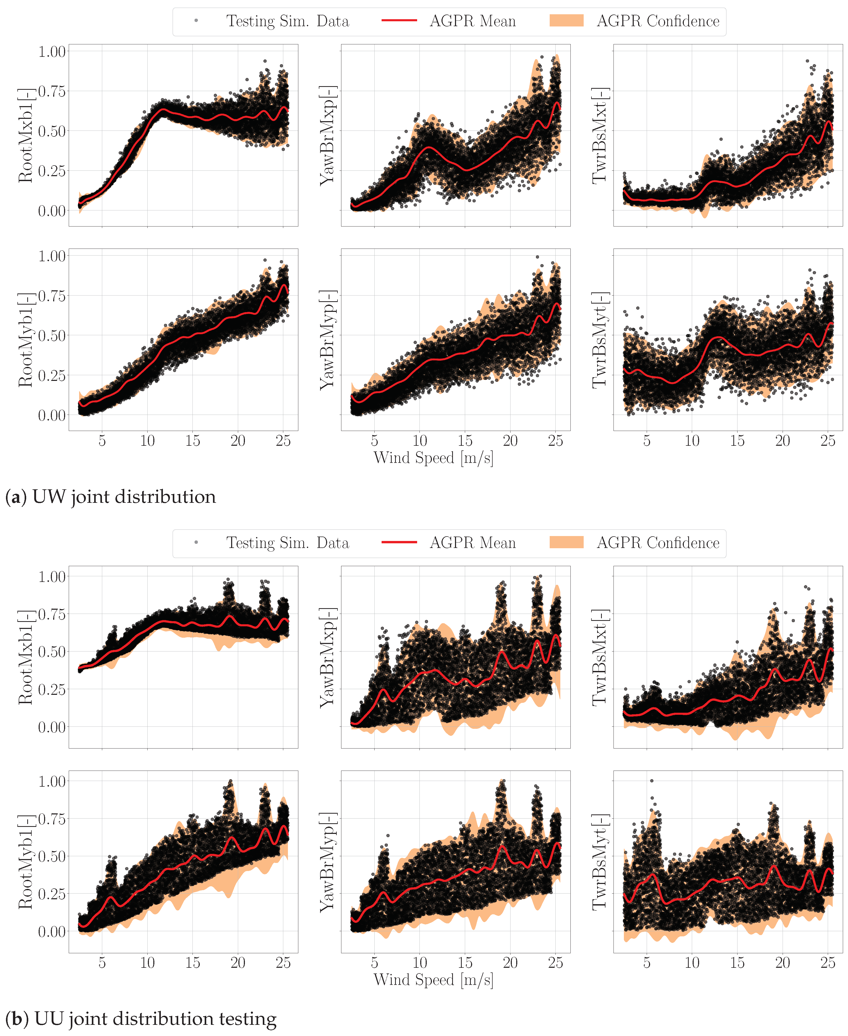
After training the AGPR models, we evaluated them by supplying a high-resolution array of wind speeds ranging from the cut-in to cut-out wind speeds. The trained models then rapidly provided the mean and STD of the DEL for each wind speed. To assess the accuracy of these models, we employed two approaches. Firstly, we plotted the evaluation process’s mean and confidence interval output alongside all the simulation testing dataset to visually assess whether the testing data fell within the confidence intervals. Secondly, we binned the simulation testing data and calculated the mean and STD of the testing QoI, as described in Section 2.1. We then determined the difference between the testing data and AGPR output using KL divergence. Figure 7a,b display the AGPR output’s mean, confidence interval, and the testing data for the DEL. In the following figures through this manuscript, the confidence interval is defined ± one STD from the AGPR mean.
Visual inspection of the plots in Figure 7 reveals that the AGPR accurately predicts the mean and confidence interval. Notably, there is a variation in turbine behavior in terms of DEL between the UW and UU cases. The UW DEL exhibits a broader output range and is less symmetrical around the mean value. Owing to this asymmetry and the symmetric nature of the confidence interval, the lower bound of the confidence interval in the UU case overshoots the testing data. The broader range of behavior in the UU case is expected, as the sampling of mean wind speed and STD fully covers the domain between the extreme minimum and maximum values per bin. Figure 7 shows some peaks in the confidence interval, particularly for the UU case, indicating a successful implementation of PLL. As explained in Section 2.5, the PLL estimates the posterior distribution of the output data. In our case, the output data has a cluster of peaks, and the posterior distribution is expanded in terms of STD to cover those wind speeds. This expansion ensures that the simulation training and testing data is adequately covered.
Table 5 presents the KL divergence between the AGPR output and the testing data for three wind speeds, with the testing data treated as the ground truth. The KL divergence is calculated according to Equation (6).
The KL divergence values in Table 5 indicate a good match between the AGPR output and the testing data. However, the AGPR is less accurate in the UU case, due to the reasons previously mentioned. Moreover, the KL divergence varies depending on the output channel and wind speed. A comparison of the plots in Figure 7 and Table 5 suggests this is primarily due to the overestimation of the STD by the AGPR. These results are typical of other wind speed bins.

3.7. AGPR Testing Results—SCADA Measurement

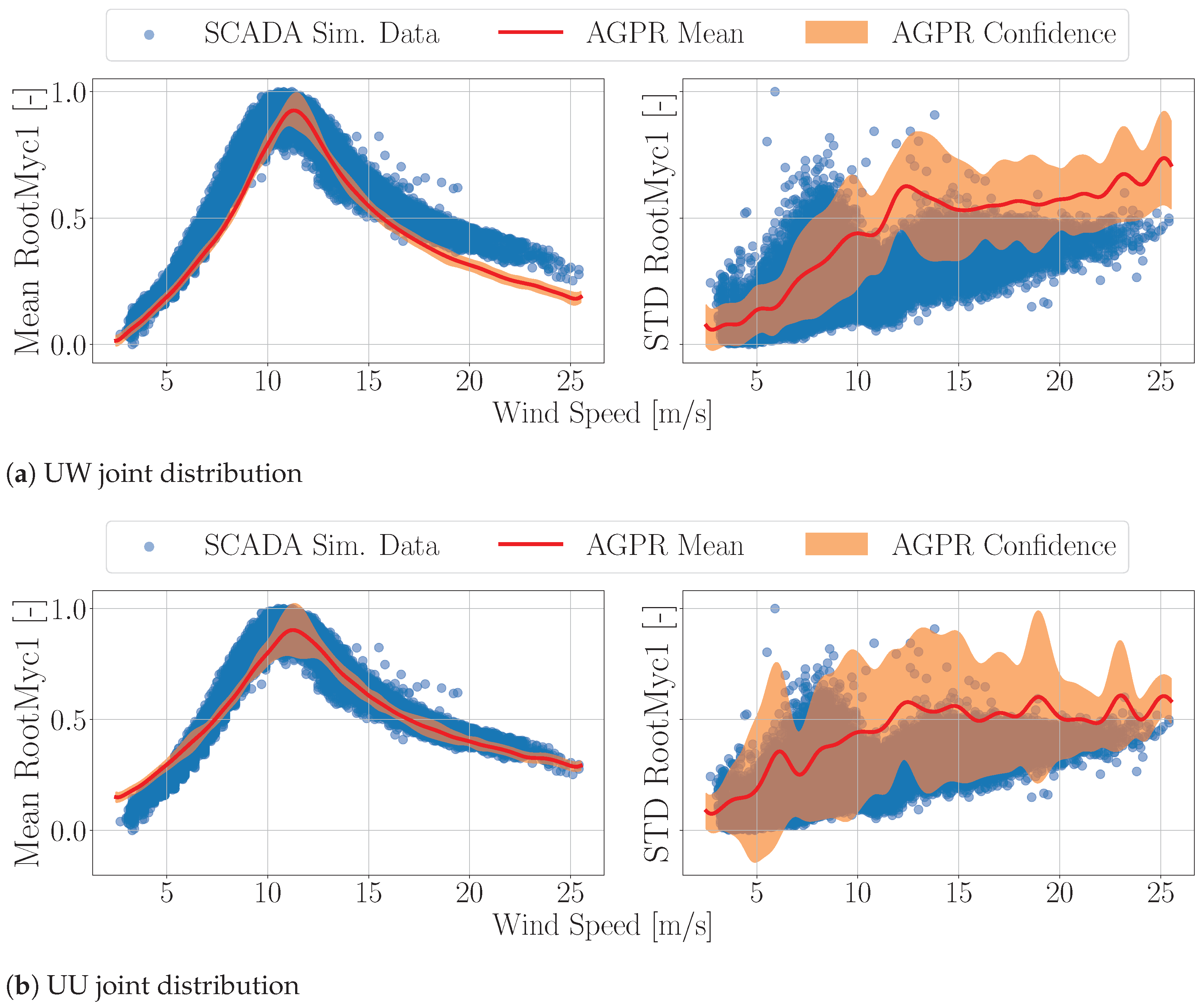
In Table 2, we provided one moment and three accelerations, each processed with a 10-min mean. These outputs correspond to the moment and acceleration available in our SCADA database, as shown in Table 1. We trained a AGPR for the 10-min mean and STD of each output based on hybrid simulations output. Subsequently, we tested the accuracy of the trained models against the corresponding mean and STD of the SCADA measurement data fields. Let us reiterate that the primary objective is to assess the effectiveness of normalized simulations of a specific simulated wind turbine in predicting the behavior of a real wind turbine machine with its own blade, controller, and structure when the real-world turbine data is proprietary and unavailable. The AGPR training settings are mentioned in Table 3. Figure 8 presents the AGPR output against the SCADA measurement for the OFP BR moment.
Despite the discrepancies in controller behavior mentioned in Section 3.5, the mean and STD of the moments from the AGPR and SCADA follow a similar pattern overall. The mean value plots in Figure 8 show that the AGPR output’s confidence interval does not entirely cover the SCADA data. This discrepancy might be attributed to the blade in the model being stiffer than in reality. This hypothesis is also supported by the STD plots, where the confidence interval of UU joint distribution provides better coverage over the SCADA data. The UU joint distribution’s broader range, which encompasses unrealistic combinations of mean wind speed and STD, results in a closer approximation of reality by the AGPR prediction. This necessity for excessive turbulence intensity is likely due to the stiffer modeled blade structure.
A noticeable peak in the mean trajectory for the STD around 6 m/s in Figure 8b is not observed in Figure 8a. A similar peak is also visible in Figure 7b for all the outputs except RootMxb1. This peak arises because the UU case models the turbine with a broader sample of STD at wind speeds around 6 m/s. According to the Campbell diagram of the NREL 5MW turbine [43], the blade passing frequency matches the side-side and fore-aft frequency of the tower at this wind speed. Typically, the STD of the wind speed does not often enter the resonance region in 10-min simulations. However, with higher turbulence, the turbine enters and exits the resonance region frequently, increasing the mean, STD, and DEL of the simulation.
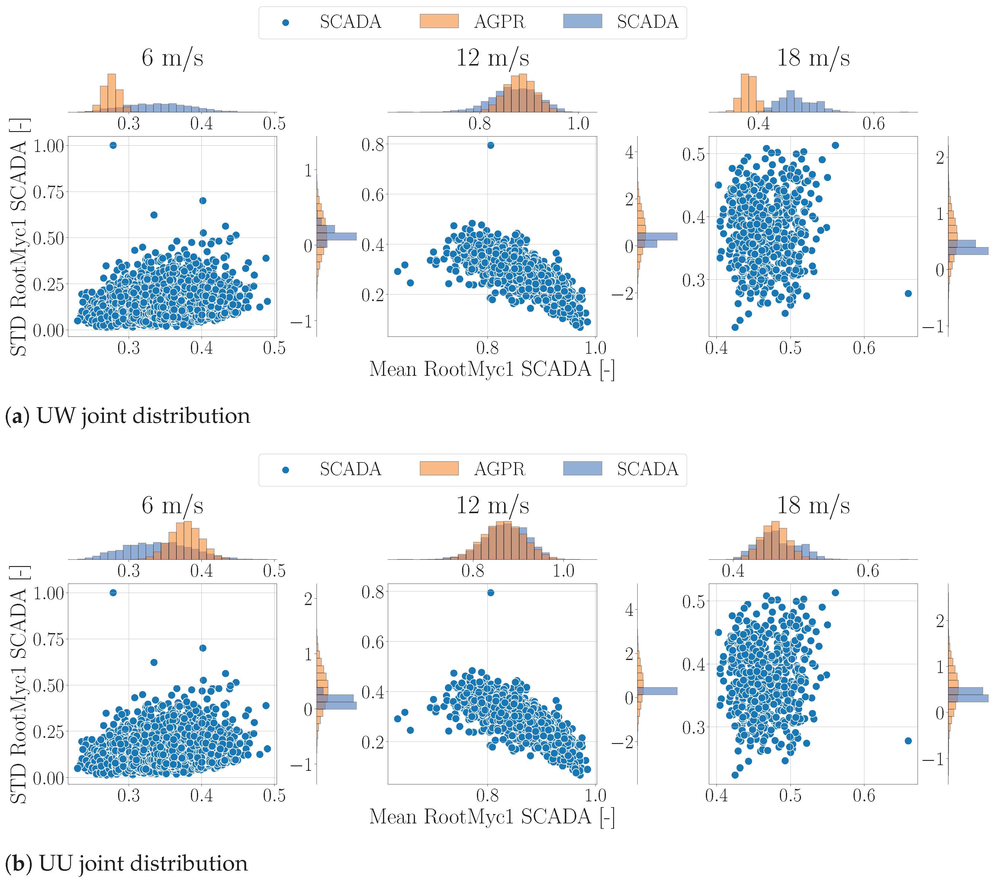
To provide a more concise comparison, Figure 9 compares the SCADA data with the AGPR predictions for three wind speeds. For each wind speed, we binned the SCADA data, as explained in Section 2.1, using the AGPR output at the bin center for comparison.
The histograms for the AGPR in Figure 9 are based on 10 5 samples from the normal distribution provided by the AGPR at the bin center. Figure 9 demonstrates that the AGPR fit varies as a function of both the wind speed and the joint distribution. The AGPR prediction of the mean value is more accurate for the UU case, but the STD prediction histogram is significantly broader than the SCADA data. This broader range is due to the manner of presenting the results: the confidence interval in Figure 8 is twice the STD, while in Figure 9, the histogram covers a wider range. It may not be a fair comparison to take the AGPR output at the center of the bin and compare it with the SCADA, which has values all over the bin. However, there are two reasons behind this. Firstly, the width of the bin for 1 m/s is narrow, and looking at Figure 8, it shows that the AGPR result and SCADA data do not change significantly in the span of 1 m/s. Therefore, one AGPR model would suffice. Secondly, as we recall from Figure 3, the measured wind speed is clustered at bins. Hence, using SCADA for one wind speed value limits the number of available data, making the statistical comparison inaccurate.
The other SCADA data fields that match the OpenFAST output is the TT resultant acceleration. Figure 10 presents the AGPR output for TT resultant acceleration trained on hybrid simulation output against the SCADA measurements.
In Figure 10, the same peak around 6 m/s observed in the mean trajectory in Figure 10b is attributable to the broader sampling of STD at wind speeds around 6 m/s as explained in Section 3.6.
Figure 10 illustrates that the UU case provides broader coverage in terms of the confidence interval due to the broader STD samples. However, the UW case more accurately follows the acceleration trend for the resultant acceleration. Assuming similar rotor thrust forces, the TT acceleration is mainly a function of the structural stiffness of the tower. A closer approximation to reality for the UW case, which is deemed more realistic for wind speed STD, suggests that the modeled tower structural stiffness is probably closer to the turbine for which we had access to the SCADA data. A more precise verification could have been achieved if we had access to tower frequency readings in the SCADA data.
We calculated the KL divergence for the OFP blade root moments and the tower top acceleration to facilitate a more precise comparison, as presented in Table 6. This calculation, based on Equation (7), uses M as the binned SCADA data described in Section 2.1, and G is derived from taking 10 5 samples from the normal distribution provided by AGPR at the center of the bin. Although Table 6 could be extended to include all wind speeds for which we have SCADA data, we have limited the presentation to three wind speeds for brevity.
Considering KL divergence as an error metric, the most accurate AGPR predictions occur for the resultant tower top accelerations in the UW case for both mean and STD. This indicates that the output of the AGPR depends on the joint distribution selected for sampling from the specific data field under examination. It also suggests that the AGPR model trained on either UW or UU may perform better depending on the data field, which is influenced by the wind turbine’s controller, aerodynamics, and structural behavior. We lack access to the model from the manufacturer, so we cannot precisely identify the reasons for the variety in AGPR performance. Nevertheless, this model and method demonstrate promising results as a primary health assessment tool.

3.8. How Can We Use This Model?

To this point, we have trained a series of AGPR models on hybrid simulations for DEL, mean, and STD. We have shown that the AGPR models trained on these hybrid simulations can accurately predict the DEL. Furthermore, we have demonstrated that the AGPR models can predict the OFP BR moments and TT accelerations from SCADA data with acceptable identification of trends. The next step is to understand how these models can be interconnected.
Figure 11 provides correlation heat maps for both UW and UU joint distributions, illustrating the correlation between DEL and the TT resultant acceleration mean.
Figure 11 shows a strong correlation between the resultant TT acceleration and the DEL loads along the tower. Except for the blade root edge-wise moment, other channels are highly or very highly correlated with the resultant accelerations. Given the high correlation between the resultant TT acceleration and the DEL, and the fidelity of the AGPR in predicting the SCADA resultant TT (Figure 10), we can hypothesize that AGPR predictions of DEL would correlate with actual DEL measurements. Although this medium level of accuracy in DEL prediction based on AGPR is insufficient for a precise health assessment, it can serve as an indicator and primary tool for diagnosing the health of wind turbine assets. During this study, we did not have access to moment measurement time series along the tower to validate this hypothesis. The authors acknowledge this limitation and recognize the need to test the hypothesis with a wind turbine instrumented with an array of sensors.

4. Conclusions

This work emphasizes the crucial need for assessing the structural health of wind turbines, given their operation in harsh environmental conditions. This assessment is vital for ensuring the longevity and optimal performance of wind turbines. The focus is on understanding the fatigue damage accumulation in these structures and the importance of advanced methods for accurate prediction and monitoring of their structural health. The methodology section details the construction of a AGPR model using a combination of the SCADA wind measurement and simulations utilizing Sobol’s sampling method. It presents a systematic method involving the generation of hybrid simulation, followed by its use in modeling and validation. The final section first explains the conditions under which the results were generated, followed by a presentation and discussion of these findings. Then, it shows the accuracy of the utilized model by comparing the simulation output and SCADA measurement for the generated power and rotor speed. Afterwards, the section shows how a AGPR trained on the hybrid simulations database accurately predicts the testing dataset and the SCADA acceleration and loads data fields. It also explores the model’s accuracy, reliability, and ability to predict potential structural issues. The results are not just numerical outputs; they are interpreted to provide insights into the overall effectiveness of the AGPR model in real-world scenarios.
This research conclusively demonstrates the efficacy and robustness of AGPR in the realm of wind turbine asset reliability. The research underscores the advanced predictive capabilities of AGPR, particularly in handling the heteroscedasticity inherent in wind turbine operational data. The ability of AGPR to accurately model and predict loads and accelerations based on a range of inputs, especially those derived from SCADA systems, while it is trained on the publicly available models and methodology is a noticeable development. It is worth noting that our tests have revealed that the choice of publicly available wind turbine model impacts the accuracy and compatibility of the trained AGPR model with the SCADA measurements. This study elaborates on how AGPR is effectively trained on hybrid simulation datasets, blending real-world measurements with simulated data to create a comprehensive model. This approach allows a better understanding of the data and enhances the model’s predictive accuracy. The research highlights the validation processes the AGPR model underwent, affirming its reliability and accuracy. The performance of the AGPR models in predicting the loads under various operational scenarios showcases its practical applicability in real-world settings. The paper points out the potential for AGPR to serve as a standard tool in the predictive maintenance of wind turbines.
While the AGPR model demonstrates promising capabilities in predicting DEL, it is important to recognize the challenges faced in this study. The lack of data about the measurement of turbine natural frequencies, dependence on specific data fields, and the limitations posed by the unavailability of the measurement wind turbine model are notable challenges. Furthermore, the transferability of the model and whether the model can be applied to various turbine types and operational scenarios, including extreme events, remains to be tested.

4.1. Future Work

Considering the fact that the model employed in this study is publicly available, and the turbine manufacturer’s model is not accessible, the performance of the AGPR for the purposes of this work is promising. For future research, there is an ambition to extend this study and test the hypothesis mentioned in Section 3.8 on a turbine equipped with sensors. Additionally, having access to more extensive and varied data fields in SCADA would be beneficial. This would help in reducing measurement uncertainties, particularly at higher wind speeds, and in fine-tuning the model for outputs that more closely reflect reality. Ideally, access to the actual wind turbine model would substantially enrich this research. Moreover, it is important to demonstrate the generalizability of this approach by implementing it on an offshore wind turbine in future work.
In the realm of data-driven modeling, we employed AGPR for this study with remarkable results. Nevertheless, exploring other methods, such as probabilistic neural networks or Bayesian neural networks, is crucial. Another avenue could involve moving away from probabilistic models and experimenting with ANNs to map environmental inputs to loads. Additionally, considering SCADA data as a time series and employing a transformer, as discussed in [60], could provide a novel approach to building a data-driven model that predicts loads based on a limited series of environmental and controller inputs.
In this study, our focus was primarily on data from power production DLCs. However, other significant events, such as shutdowns, gusts, and faults during a wind turbine’s lifetime, can impact its structural integrity. These scenarios are crucial and should be considered in future studies.

Author Contributions

R.H. and C.S. developed the idea under the supervision of C.C. R.H. built and processed the hybrid and SCADA databases. C.S. and R.H. developed the necessary computer code. R.H. wrote the paper in consultation with and under the supervision of C.C. All authors have read and agreed to the published version of the manuscript.

Funding

We greatly acknowledge the funding for this study by the Natural Sciences and Engineering Research Council of Canada (NSERC) and MiTACS.

Data Availability Statement

The SCADA data and hybrid databases are unavailable due to NDA. The developed code for GPR is available upon request.

Acknowledgments

This research was partly enabled by support provided by the Digital Research Alliance of Canada (alliancecan.ca). We want to thank John Wang and Selena Farris from Clir for providing us with SCADA datasets and giving us feedback during this study.

Conflicts of Interest

The authors declare no conflicts of interest.

References

  1. Ciang, C.C.; Lee, J.R.; Bang, H.J. Structural Health Monitoring for a Wind Turbine System: A Review of Damage Detection Methods. Meas. Sci. Technol. 2008, 19, 122001. [Google Scholar] [CrossRef]
  2. Martinez-Luengo, M.; Kolios, A.; Wang, L. Structural Health Monitoring of Offshore Wind Turbines: A Review through the Statistical Pattern Recognition Paradigm. Renew. Sustain. Energy Rev. 2016, 64, 91–105. [Google Scholar] [CrossRef]
  3. Yang, W.; Tavner, P.J.; Crabtree, C.J.; Feng, Y.; Qiu, Y. Wind Turbine Condition Monitoring: Technical and Commercial Challenges. Wind Energy 2014, 17, 673–693. [Google Scholar] [CrossRef]
  4. Tchakoua, P.; Wamkeue, R.; Ouhrouche, M.; Slaoui-Hasnaoui, F.; Tameghe, T.A.; Ekemb, G. Wind Turbine Condition Monitoring: State-of-the-Art Review, New Trends, and Future Challenges. Energies 2014, 7, 2595–2630. [Google Scholar] [CrossRef]
  5. Leahy, K.; Gallagher, C.; O’Donovan, P.; O’Sullivan, D.T.J. Issues with Data Quality for Wind Turbine Condition Monitoring and Reliability Analyses. Energies 2019, 12, 201. [Google Scholar] [CrossRef]
  6. Badrzadeh, B.; Bradt, M.; Castillo, N.; Janakiraman, R.; Kennedy, R.; Klein, S.; Smith, T.; Vargas, L. Wind Power Plant SCADA and Controls. In Proceedings of the 2011 IEEE Power and Energy Society General Meeting, Detroit, MI, USA, 24–28 July 2011; pp. 1–7. [Google Scholar] [CrossRef]
  7. Marti-Puig, P.; Blanco-M., A.; Serra-Serra, M.; Solé-Casals, J. Wind Turbine Prognosis Models Based on SCADA Data and Extreme Learning Machines. Appl. Sci. 2021, 11, 590. [Google Scholar] [CrossRef]
  8. Tautz-Weinert, J.; Watson, S.J. Using SCADA Data for Wind Turbine Condition Monitoring—A Review. IET Renew. Power Gener. 2017, 11, 382–394. [Google Scholar] [CrossRef]
  9. Toft, H.S.; Svenningsen, L.; Moser, W.; Sørensen, J.D.; Thøgersen, M.L. Assessment of Wind Turbine Structural Integrity Using Response Surface Methodology. Eng. Struct. 2016, 106, 471–483. [Google Scholar] [CrossRef]
  10. Stewart, G. Design Load Analysis of Two Floating Offshore Wind Turbine Concepts. Doctoral Dissertation, University of Massachusetts Amherst, Amherst, MA, USA, 2016. [Google Scholar] [CrossRef]
  11. Teixeira, R.; O’Connor, A.; Nogal, M.; Krishnan, N.; Nichols, J. Analysis of the Design of Experiments of Offshore Wind Turbine Fatigue Reliability Design with Kriging Surfaces. Procedia Struct. Integr. 2017, 5, 951–958. [Google Scholar] [CrossRef]
  12. Müller, K.; Dazer, M.; Cheng, P.W. Damage Assessment of Floating Offshore Wind Turbines Using Response Surface Modeling. Energy Procedia 2017, 137, 119–133. [Google Scholar] [CrossRef]
  13. Müller, K.; Cheng, P.W. Application of a Monte Carlo Procedure for Probabilistic Fatigue Design of Floating Offshore Wind Turbines. Wind Energy Sci. 2018, 3, 149–162. [Google Scholar] [CrossRef]
  14. Dimitrov, N.; Kelly, M.C.; Vignaroli, A.; Berg, J. From Wind to Loads: Wind Turbine Site-Specific Load Estimation with Surrogate Models Trained on High-Fidelity Load Databases. Wind Energy Sci. 2018, 3, 767–790. [Google Scholar] [CrossRef]
  15. Haghi, R.; Crawford, C. Surrogate Models for the Blade Element Momentum Aerodynamic Model Using Non-Intrusive Polynomial Chaos Expansions. Wind Energy Sci. 2022, 7, 1289–1304. [Google Scholar] [CrossRef]
  16. Schröder, L.; Dimitrov, N.K.; Verelst, D.R. A Surrogate Model Approach for Associating Wind Farm Load Variations with Turbine Failures. Wind Energy Sci. 2020, 5, 1007–1022. [Google Scholar] [CrossRef]
  17. Dimitrov, N.; Göçmen, T. Virtual Sensors for Wind Turbines with Machine Learning-Based Time Series Models. Wind Energy 2022, 25, 1626–1645. [Google Scholar] [CrossRef]
  18. Maldonado-Correa, J.; Martín-Martínez, S.; Artigao, E.; Gómez-Lázaro, E. Using SCADA Data for Wind Turbine Condition Monitoring: A Systematic Literature Review. Energies 2020, 13, 3132. [Google Scholar] [CrossRef]
  19. Gonzalez, E.; Stephen, B.; Infield, D.; Melero, J.J. Using High-Frequency SCADA Data for Wind Turbine Performance Monitoring: A Sensitivity Study. Renew. Energy 2019, 131, 841–853. [Google Scholar] [CrossRef]
  20. Gray, C.S.; Watson, S.J. Physics of Failure Approach to Wind Turbine Condition Based Maintenance. Wind Energy 2010, 13, 395–405. [Google Scholar] [CrossRef]
  21. Galinos, C.; Dimitrov, N.; Larsen, T.J.; Natarajan, A.; Hansen, K.S. Mapping Wind Farm Loads and Power Production—A Case Study on Horns Rev 1. J. Phys. Conf. Ser. 2016, 753, 032010. [Google Scholar] [CrossRef]
  22. Alvarez, E.J.; Ribaric, A.P. An Improved-Accuracy Method for Fatigue Load Analysis of Wind Turbine Gearbox Based on SCADA. Renew. Energy 2018, 115, 391–399. [Google Scholar] [CrossRef]
  23. Remigius, W.D.; Natarajan, A. Identification of Wind Turbine Main-Shaft Torsional Loads from High-Frequency SCADA (Supervisory Control and Data Acquisition) Measurements Using an Inverse-Problem Approach. Wind Energy Sci. 2021, 6, 1401–1412. [Google Scholar] [CrossRef]
  24. Pandit, R.; Astolfi, D.; Hong, J.; Infield, D.; Santos, M. SCADA Data for Wind Turbine Data-Driven Condition/Performance Monitoring: A Review on State-of-Art, Challenges and Future Trends. Wind Eng. 2023, 47, 422–441. [Google Scholar] [CrossRef]
  25. Vera-Tudela, L.; Kühn, M. Analysing Wind Turbine Fatigue Load Prediction: The Impact of Wind Farm Flow Conditions. Renew. Energy 2017, 107, 352–360. [Google Scholar] [CrossRef]
  26. Natarajan, A.; Bergami, L. Determination of Wind Farm Life Consumption in Complex Terrain Using Ten-Minute SCADA Measurements. J. Phys. Conf. Ser. 2020, 1618, 022013. [Google Scholar] [CrossRef]
  27. Mylonas, C.; Abdallah, I.; Chatzi, E. Conditional Variational Autoencoders for Probabilistic Wind Turbine Blade Fatigue Estimation Using Supervisory, Control, and Data Acquisition Data. Wind Energy 2021, 24, 1122–1139. [Google Scholar] [CrossRef]
  28. Rasmussen, C.E.; Williams, C.K.I. Gaussian Processes for Machine Learning; The MIT Press: Cambridge, MA, USA, 2005. [Google Scholar] [CrossRef]
  29. Pandit, R.K.; Infield, D. SCADA-based Wind Turbine Anomaly Detection Using Gaussian Process Models for Wind Turbine Condition Monitoring Purposes. IET Renew. Power Gener. 2018, 12, 1249–1255. [Google Scholar] [CrossRef]
  30. Li, Y.; Liu, S.; Shu, L. Wind Turbine Fault Diagnosis Based on Gaussian Process Classifiers Applied to Operational Data. Renew. Energy 2019, 134, 357–366. [Google Scholar] [CrossRef]
  31. Herp, J.; Ramezani, M.H.; Bach-Andersen, M.; Pedersen, N.L.; Nadimi, E.S. Bayesian State Prediction of Wind Turbine Bearing Failure. Renew. Energy 2018, 116, 164–172. [Google Scholar] [CrossRef]
  32. Avendaño-Valencia, L.D.; Abdallah, I.; Chatzi, E. Virtual Fatigue Diagnostics of Wake-Affected Wind Turbine via Gaussian Process Regression. Renew. Energy 2021, 170, 539–561. [Google Scholar] [CrossRef]
  33. Wilkie, D.; Galasso, C. Gaussian Process Regression for Fatigue Reliability Analysis of Offshore Wind Turbines. Struct. Saf. 2021, 88, 102020. [Google Scholar] [CrossRef]
  34. Singh, D.; Dwight, R.P.; Laugesen, K.; Beaudet, L.; Viré, A. Probabilistic Surrogate Modeling of Offshore Wind-Turbine Loads with Chained Gaussian Processes. J. Phys. Conf. Ser. 2022, 2265, 032070. [Google Scholar] [CrossRef]
  35. Kuhn, M.; Johnson, K. Feature Engineering and Selection: A Practical Approach for Predictive Models; CRC Press: Bocca Raton, FL, USA, 2020; Available online: http://www.feat.engineering/ (accessed on 15 September 2023).
  36. Daley, R. Atmospheric Data Analysis; Number 2; Cambridge University Press: Cambridge, UK, 1993. [Google Scholar]
  37. Sobol’, I.M. On the Distribution of Points in a Cube and the Approximate Evaluation of Integrals. USSR Comput. Math. Math. Phys. 1967, 7, 86–112. [Google Scholar] [CrossRef]
  38. Kucherenko, S.; Albrecht, D.; Saltelli, A. Exploring Multi-Dimensional Spaces: A Comparison of Latin Hypercube and Quasi Monte Carlo Sampling Techniques. arXiv 2015, arXiv:1505.02350. [Google Scholar]
  39. Renardy, M.; Joslyn, L.R.; Millar, J.A.; Kirschner, D.E. To Sobol or Not to Sobol? The Effects of Sampling Schemes in Systems Biology Applications. Math. Biosci. 2021, 337, 108593. [Google Scholar] [CrossRef] [PubMed]
  40. Jonkman, B.J.; Buhl, M.L., Jr. TurbSim User’s Guide: Version 1.50; Technical Report NREL/TP–500-46198; National Renewable Energy Lab. (NREL): Golden, CO, USA, 2009. Available online: https://www.nrel.gov/docs/fy09osti/46198.pdf (accessed on 15 September 2023).
  41. Jonkman, B.; Mudafort, R.M.; Platt, A.; Branlard, E.; Sprague, M.; Jjonkman; HaymanConsulting; Hall, M.; Vijayakumar, G.; Buhl, M.; et al. OpenFAST/openfast: OpenFAST v3.3.0. Zenodo, 28 October 2022. Available online: https://zenodo.org/records/7262094 (accessed on 15 September 2023).
  42. IEC 61400-1:2019; Wind Energy Generation Systems—Part 1: Design Requirements. International Electrotechnical Commission: Geneva, Switzerland, 2019.
  43. Jonkman, J.; Butterfield, S.; Musial, W.; Scott, G. Definition of a 5-MW Reference Wind Turbine for Offshore System Development; Technical Report; National Renewable Energy Lab. (NREL): Golden, CO, USA, 2009.
  44. Rinker, J.; Dykes, K. WindPACT Reference Wind Turbines; Technical Report NREL/TP–5000-67667, 1432194; National Renewable Energy Laboratory (NREL): Golden, CO, USA, 2018. [CrossRef]
  45. Bortolotti, P.; Tarres, H.C.; Dykes, K.; Merz, K.; Sethuraman, L.; Verelst, D.; Zahle, F. IEA Wind Task 37 on Systems Engineering in Wind Energy—WP2.1 Reference Wind Turbines; Technical Report; International Energy Agency: Paris, France, 2019. [Google Scholar]
  46. Quon, E. NREL/Openfast-Turbine-Models: A Repository of OpenFAST Turbine Models Developed by NREL Researchers. 2021. GitHub Repository. Available online: https://github.com/NREL/openfast-turbine-models/tree/master (accessed on 15 September 2023).
  47. Thomsen, K. The Statistical Variation of Wind Turbine Fatigue Loads; Number 1063 in Risø-R; Risø National Laboratory: Roskilde, Denmark, 1998.
  48. Stiesdal, H. Rotor Loadings on the BONUS 450 kW Turbine. J. Wind Eng. Ind. Aerodyn. 1992, 39, 303–315. [Google Scholar] [CrossRef]
  49. Matsuishi, M.; Endo, T. Fatigue of metals subjected to varying stress. Jpn. Soc. Mech. Eng. Fukuoka Jpn. 1968, 68, 37–40. [Google Scholar]
  50. Quiñonero-Candela, J.; Rasmussen, C.E.; Williams, C.K.I. Approximation Methods for Gaussian Process Regression. In Large-Scale Kernel Machines; Bottou, L., Chapelle, O., DeCoste, D., Weston, J., Eds.; The MIT Press: Cambridge, MA, USA, 2007; pp. 203–224. [Google Scholar] [CrossRef]
  51. Kersting, K.; Plagemann, C.; Pfaff, P.; Burgard, W. Most Likely Heteroscedastic Gaussian Process Regression. In Proceedings of the 24th International Conference on Machine Learning, Corvalis, OR, USA, 20–24 June 2007; pp. 393–400. [Google Scholar] [CrossRef]
  52. Jankowiak, M.; Pleiss, G.; Gardner, J. Parametric Gaussian Process Regressors. In Proceedings of the 37th International Conference on Machine Learning, Virtual, 13–18 July 2020; pp. 4702–4712. [Google Scholar]
  53. Hensman, J.; Matthews, A.; Ghahramani, Z. Scalable Variational Gaussian Process Classification. In Proceedings of the Eighteenth International Conference on Artificial Intelligence and Statistics, San Diego, CA, USA, 9–12 May 2015; pp. 351–360. [Google Scholar]
  54. Gardner, J.; Pleiss, G.; Weinberger, K.Q.; Bindel, D.; Wilson, A.G. GPyTorch: Blackbox Matrix-Matrix Gaussian Process Inference with GPU Acceleration. In Proceedings of the Advances in Neural Information Processing Systems, Montréal, QC, Canada, 3–8 December 2018; Volume 31. [Google Scholar]
  55. Murphy, K.P. Machine Learning: A Probabilistic Perspective; Adaptive Computation and Machine Learning Series; MIT Press: Cambridge, MA, USA, 2012. [Google Scholar]
  56. Owen, A.B. On Dropping the First Sobol’ Point. arXiv 2021, arXiv:2008.08051. [Google Scholar]
  57. Jonkman, J.M.; Buhl, M.L., Jr. Fast User’s Guide-Updated August 2005; Technical Report NREL/TP–500-38230; National Renewable Energy Lab. (NREL): Golden, CO, USA, 2005. Available online: https://www.nrel.gov/docs/fy06osti/38230.pdf (accessed on 15 September 2023).
  58. Branlard, E. pyfast. 2023. GitHub Repository. Available online: https://github.com/OpenFAST/python-toolbox (accessed on 15 September 2023).
  59. Lever, J.; Krzywinski, M.; Altman, N. Model Selection and Overfitting. Nat. Methods 2016, 13, 703–704. [Google Scholar] [CrossRef]
  60. Vaswani, A.; Shazeer, N.; Parmar, N.; Uszkoreit, J.; Jones, L.; Gomez, A.N.; Kaiser, L.; Polosukhin, I. Attention Is All You Need. In Proceedings of the Advances in Neural Information Processing Systems, Beach, CA, USA, 4–9 December 2017; Volume 30. [Google Scholar]
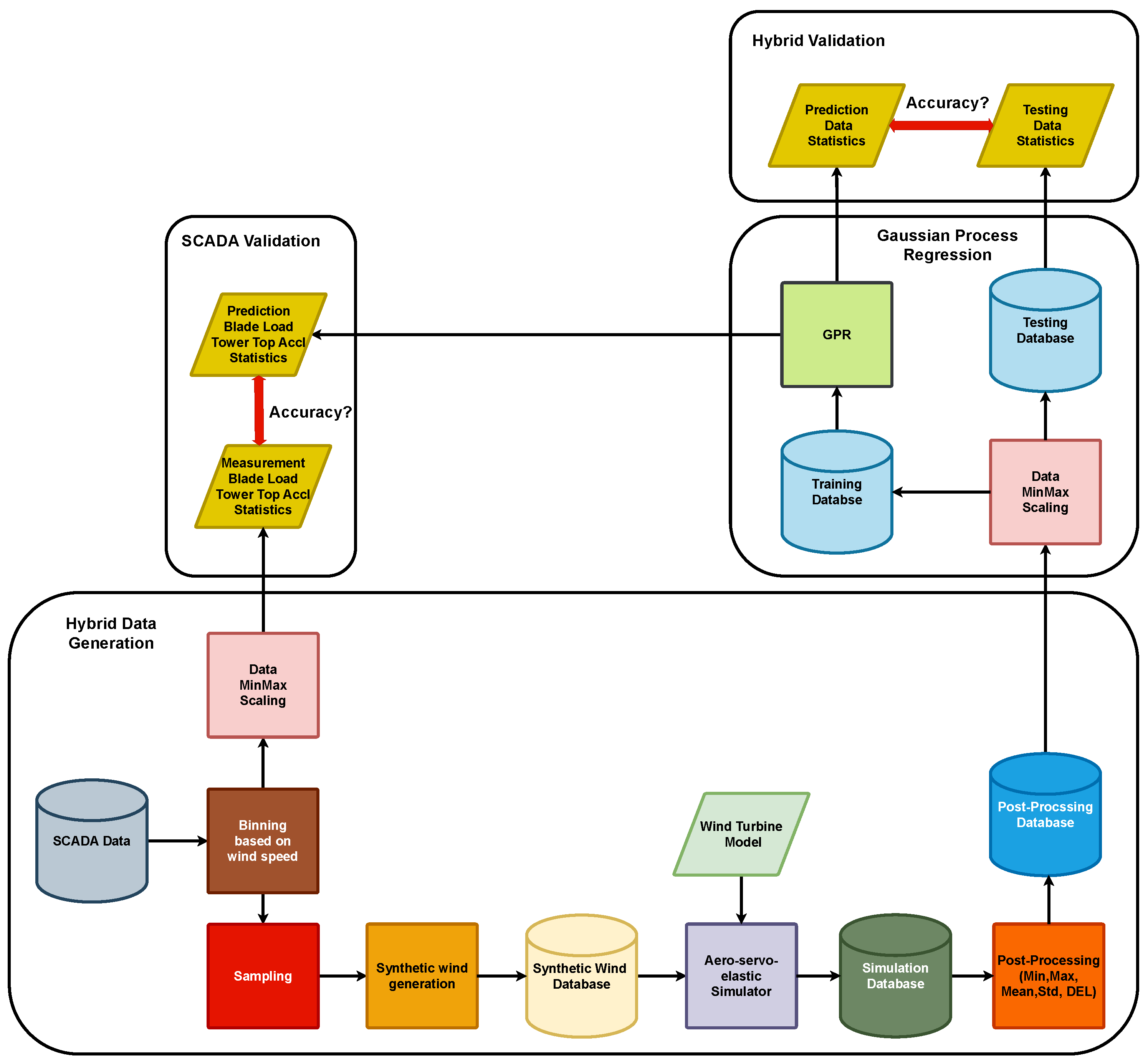
Figure 1. The methodology employed in this manuscript.
Energies 17 00346 g001
Figure 2. Illustration of SCADA Measurement Data: The top right panel shows raw data for mean and STD wind speeds. The diagonal panels feature histograms for both mean wind speed and STD wind speed, accordingly. The bottom left panel presents a 2D histogram, elucidating the relationship between mean wind speed and STD wind speed measurements.
Energies 17 00346 g002
Figure 3. A total of 512 Sobol’s samples example for the 20 m/s wind speed bin for the UW and UU options.
Energies 17 00346 g003
Figure 4. (a,b) present the schematic depiction of the turbine highlighting the moment output load channel locations. The red arrows depict the moments according to OpenFAST [46].
Energies 17 00346 g004
Figure 5. Comparison of SCADA-measured and simulated power generation for UW and UU joint distributions.
Energies 17 00346 g005
Figure 6. Comparison of SCADA-measured and simulated rotor speed for UW and UU joint distributions.
Energies 17 00346 g006
Figure 7. The AGPR outputs and simulation testing data for UW and UU joint distributions.
Energies 17 00346 g007
Figure 8. OFP BR AGPR prediction vs. the SCADA data.
Energies 17 00346 g008
Figure 9. OFP BR AGPR prediction vs. the SCADA for three wind speeds. The histogram represents the probability density.
Energies 17 00346 g009
Figure 10. TT resultant acceleration AGPR prediction vs. the SCADA data.
Energies 17 00346 g010
Figure 11. Hybrid simulations correlation heat map. The rows represent the DEL values.
Energies 17 00346 g011
Table 1. The SCADA data fields used in this study. The abbreviations are tower-top (TT) and out-of-plane (OFP), while Res. is short for resultant and accel. for acceleration.
DatafieldUnit10-min Avg10-min STD10-min Min10-min Max
Power[kW]-
Rotor Speed[rpm]-
OFP blade load[Nm]
TT Res. accel.[mm/s2]
Table 2. List of channel descriptions and the adopted naming and units.
OpenFAST Channel LabelAdopted NamePost-ProcessingUnit
GenPwrPower Output10-min mean[kW]
RtSpeedRotor Speed10-min mean[kW]
RootMyc1Out-of-plane BR moment10-min mean[kNm]
YawBrTAxpTT fore-aft acceleration10-min mean[m/s2]
YawBrTAypTT side-side acceleration10-min mean[m/s2]
YawBrTAcclTT resultant acceleration10-min mean[m/s2]
RootMxb1Edge-wise BR momentDEL[kNm]
RootMyb1Flap-wise BR momentDEL[kNm]
YawBrMxpTT side-sideDEL[kNm]
YawBrMypTT fore-aftDEL[kNm]
TwrBsMxtTB side-sideDEL[kNm]
TwrBsMytTB fore-aftDEL[kNm]
Table 3. GPyTorch configurations for AGPR model training on DEL and 10-min mean values.
DEL10 min MeanReference
Model classApproximate GPApproximate GP[50]
Kernel (length scale)RBF Kernel (0.7)RBF Kernel (0.7)[28]
Marginal likelihood classPLLPLL[52]
Variational distributionCholeskyCholesky[54]
Training dataset size588811,776-
Number of inducing points6464-
Number of iterations500500-
Table 4. Difference between binned scaled simulated power and measured power in percentage across a selection of wind speeds for UW and UU joint distributions.
Wind Speed [m/s]Uniform-Weibull [%]Uniform-Uniform [%]
300
58.6326.86
10−11.99−10.97
152.652.17
206.206.20
2525.0325.02
Table 5. KL divergence for three wind speeds comparing testing data and AGPR output.
  UW [-]   UU [-] 
Channels 6 m/s 12 m/s 18 m/s   6 m/s 12 m/s 18 m/s
RootMxb10.0290.0000.024 0.0020.0040.042
RootMyb10.0100.0090.014 0.0030.0010.005
YawBrMxp0.0430.0130.001 0.0020.0050.024
YawBrMyp0.0040.0070.020 0.0030.0010.013
TwrBsMxt0.0090.0250.005 0.0010.0000.003
TwrBsMyt0.0020.0000.011 0.0050.0040.001
Table 6. KL divergence for three wind speeds comparing binned SCADA and AGPR center bin output.
  UW [-]   UU [-] 
Data Field 6 m/s 12 m/s 18 m/s   6 m/s 12 m/s 18 m/s
OFP BR Moment mean1.7830.1609.317 0.7010.0320.184
OFP BR Moment STD3.0065.5565.736 3.6836.1965.487
TT Res. accl. mean1.6800.2530.915 5.3580.8891.539
TT Res. accl. STD2.3630.2520.625 5.5111.6192.884
Disclaimer/Publisher’s Note: The statements, opinions and data contained in all publications are solely those of the individual author(s) and contributor(s) and not of MDPI and/or the editor(s). MDPI and/or the editor(s) disclaim responsibility for any injury to people or property resulting from any ideas, methods, instructions or products referred to in the content.