Combined K-Means Clustering with Neural Networks Methods for PV Short-Term Generation Load Forecasting in Electric Utilities

Abstract

The power system has undergone significant growth and faced considerable challenges in recent decades, marked by the surge in energy demand and advancements in smart grid technologies, including solar and wind energies, as well as the widespread adoption of electric vehicles. These developments have introduced a level of complexity for utilities, compounded by the rapid expansion of behind-the-meter (BTM) photovoltaic (PV) systems, each with its own unique design and characteristics, thereby impacting power grid stability and reliability. In response to these intricate challenges, this research focused on the development of a robust forecasting model for load generation. This precision forecasting is crucial for optimal planning, mitigating the adverse effects of PV systems, and reducing operational and maintenance costs. By addressing these key aspects, the goal is to enhance the overall resilience and efficiency of the power grid amidst the evolving landscape of energy and technological advancements. The authors propose a solution leveraging LSTM (long short-term memory) model for a forecasting horizon up to 168 hours. This approach incorporates combinations of K-means clustering, automated meter infrastructure (AMI) real-world PV load generation, weather data, and calculated solar positions to forecast the generation load at customer locations to achieve a 5.7% mean absolute error between the actual and the predicted generation load.

1. Introduction

Electricity generation systems have traditionally been dominated by fossil fuel-based generators. Yet, because of these generators’ detrimental effects on the environment, the power industry is currently concentrating on green energy-based alternative generation technologies [1]. Solar energy photovoltaics (PVs) is one of the most desirable green energies among the many renewable energy resources, since it has environmental and economic benefits [2]. In addition, the U.S. Department of Solar Energy Technologies Office (SETO) and the National Renewable Energy Laboratory (NREL) developed a solar future study, the findings of which were that solar will grow from 3% of the U.S. electricity supply today to 40% by 2035 to become 95% decarbonized, and 45% by 2050 to achieve 100% decarbonization [3]. However, the integration of solar PVs has added significant issues to the power grid such as the system stability, reliability, electric power balance, reactive power compensation, and frequency response. Solar PV generation forecasting has emerged as an effective solution to address these problems [4,5].

This manuscript is designed for the electric utility industry. It explores the importance of precise solar forecasting in various aspects of photovoltaic (PV) system management and operation. The accurate prediction of solar energy output offers numerous benefits, including the reduction of auxiliary device maintenance costs, increased PV system penetration, mitigation of the impact of an uncertain solar PV output, and enhanced overall system stability. By utilizing advanced approaches, such as neural network machine learning models, AMI real-world PV generation data, and weather data, the proposed methodologies for PV solar load forecasting provide additional industry-specific advantages. These include an enhanced accuracy in load estimation, facilitating optimal planning and resource allocation. Moreover, the improved forecasting accuracy helps minimize operational and maintenance costs, ensuring efficient utilization of PV systems. Furthermore, it enables a better integration of renewable energy sources such as solar PV, optimizing their contribution to the overall energy mix and promoting a more sustainable energy landscape. With the application of these approaches, the industry can achieve better operational efficiency, cost savings, and a reliable power grid while harnessing the full potential of solar energy resources. The key areas of focus in this study are the development of forecasting methodologies for solar PV power generation. These methodologies aim to optimize the utilization of solar energy by effectively predicting the amount of power that can be generated from PV systems. The forecasting models employed in this research consider several factors such as the solar position based on the geographic location and climatic variability. The optimum features and model hyper parameters were chosen using input parameter selection and training procedures.

To achieve accurate short-term solar forecasting, machine learning techniques are analyzed and compared in this manuscript. Machine learning has proven to be an effective tool in capturing complex patterns and relationships within solar data, enabling more precise predictions. By evaluating and comparing different machine learning algorithms, this study aims to identify the most suitable approach for solar PV generation load forecasting.

To ensure the effective integration of solar power into the energy grid, fostering grid stability, and advancing toward a more sustainable future and optimal planning, the contributions of this paper are as follows:

(1)

We engineered an integrated model, combining K-means clustering with LSTM, where a sequence of nine features and load generation were utilized for the purpose of forecasting solar generation across a horizon extending up to 168 hours. This combined approach leverages the strengths of both clustering and sequential modeling techniques to enhance the accuracy and robustness of the predictive capabilities of solar energy generation.

(2)

The model was specifically tailored for electric utilities. It is intended to be integrated into electric utility systems that utilize automated meter infrastructure (AMI) data for their operational processes.

(3)

We utilized real electric utility AMI data collected from customer locations and compared the model’s performance with multiple widely used algorithms in the context of photovoltaic power forecasting.

(4)

We reduced the daytime mean absolute error between the actual and the forecasted load generation from 14.3% to 5.7% in all weather conditions and achieved excellent results in comparison with the best models.

The remainder of this manuscript is organized as follows: In Section 2, we highlight related work in solar generation forecasting techniques. In Section 3, we present our methodology, which consists of data processing and forecast models. In Section 4, we give the results for each model and evaluate the performance. In Section 5, conclusions and future work are discussed. The references used in the article are in the last section.

2. Related Work

Energy forecasting is a well-known and long-standing concern in power systems. Nevertheless, with advances in artificial intelligence and machine learning over the past ten years, as well as the expansion of distributed energy resources, load forecasting has emerged as a key issue. There are different methodologies for energy forecasting. They can be classified into time-series models, regression models, and artificial neural networks models [6].

The classic linear time-series models mainly include autoregressive (AR) models, moving average (MA) models, autoregressive moving average (ARMA) models, and autoregressive integrated moving average (ARIMA) models. They are widely used for the prediction of stationary time-series data [7]. However, the main challenges of these models are the high complexity of time series data, low accuracy, and poor generalization ability of the prediction model [8]. These models were proposed in [9].

Regression models can be developed for different time ranges (short, medium, and long term) considering different influential environmental and temporal parameters [10]. Linear regression (LR) models are widely used in energy forecasting since they are simple and effective [11]. Another regression technique is support vector regression (SVR); it was developed to provide a relationship between two nonlinear variables. However, SVR has a limitation: it inherently provides only a one-step-ahead forecast by default. To address this, various strategies have been implemented, but they often lead to data loss, introduce additional errors, or become computationally expensive [12]. In [13,14], the regression models including SVR were discussed and proposed. Artificial neural networks (ANNs) can be used to create models for complex nonlinear processes using input variables that are correlated, without making any assumptions about the underlying process [15]; thus, these models were explored for solar power forecasting and are applied in [16,17,18].

In modern research focusing on mathematical modeling for renewable energy systems, artificial neural networks (ANNs) play a pivotal role. Studies have demonstrated that ANNs yield superior solar forecasting outcomes compared to conventional statistical approaches [19]. The multilayer perceptron structure (MLP) is the most frequently encountered neural network [20]; its performance is often constrained by its reliance on one-to-one relationships between the input and the output. This limitation becomes apparent as MLPs do not inherently account for the sequential characteristics present in time-series data, thus hindering their forecasting accuracy [21]. The deep learning or deep neural network (DNN) has emerged in recent years; it is a development of neural networks with improved capacity to solve complex problems. A deep learning framework to predict PV power forecasting was discussed in [22,23]. Long short-term memory (LSTM), which is a recurrent neural network (RNN), is a type of deep learning network that has been widely utilized in time-series forecasting and has shown powerful results [24]; this type of deep learning has been proven and demonstrated as highly effective models for several challenging learning tasks [25]. Convolutional neural networks (CNNs), which were originally designed for image recognition, have been performing well in load predictions, and have the ability to extract spatial features [26]. A methodology based on the CNN for short-term load forecasting is proposed in [27]. Hybrid models, which are combinations of different types of neural networks, proposed in [28,29] were compared with different methodologies. Notably, these hybrid models outperformed regression-based methods, highlighting their efficacy in enhancing forecasting accuracy. Ensemble techniques are methodologies to combine predictions from multiple models to produce a single forecast. An ensemble approach is proposed in [30] to develop forecasting models for energy consumption and energy generation of household communities.

While many approaches have been proposed for load forecasting, there are still areas that have not been fully explored. Some potential areas for further development in load forecasting include incorporating more diverse data sources that can be leveraged, such as social media or building occupancy data, to improve the forecasting accuracy. Load forecasting models assume that the statistical properties of the load data remain constant over time, but load patterns can change due to changes in consumer behavior, technological advances, or other factors. Developing methods to account for non-stationarity in load data could improve the forecasting accuracy. Uncertainty is inherent in load forecasting, and incorporating methods to quantify and address this uncertainty could improve decision-making. Although load forecasting has traditionally been used for energy management, it could potentially be useful in other areas such as traffic management or supply chain optimization.

Table 1. Comparison of short-term generation load methodologies in top-cited journals.

Reference Number	Forecasting Model	Smart Meter Data	Multiple Locations	Forecast Horizon	Limitations
[31]	Probabilistic	no	yes	1 h ahead	Did not use weather data
[32]	ARX (AutoRegressive with eXogenous)	yes	yes	2 h ahead	Large number of missing data, not enough data to evaluate cloudy and rainy days.
[33]	Gradient Boosting trees	no	yes	72 h ahead	Uses NWP data, which are complicated and highly expensive [34]
[35]	SOM (Self-Organizing Map) and Fuzzy	yes	no	24 h ahead	Forecasts worse on typhoon days, need more data collection
[36]	SVR (Support Vector Regression)	no	no	24 h ahead	Used automatic data logger, which has limited memory capacity and lacks real-time data
[37]	Gaussian Process Regression	no	no	<1 h	Only 33 days used for training which affected the performance, high computational process
[38]	Autoregression	no	yes	6 h ahead	Used weather satellite images which are complex and expensive
[39]	Neural Network Ensemble	no	no	24 h ahead	Not sufficient training data samples, which affected the forecast performance
This article	K-means clustering with Linear Regression, Deep Neural Network, and LSTM	yes	yes	168 h ahead	Uses actual electric utility data

compares different methods used in the top-cited journals for short-term solar generation load forecasting. The methods are evaluated on four criteria: whether the models used smart meter data, whether the research data were obtained from multiple locations, the forecast horizon, and the limitations of each article.

Our model uses AMI smart meter data, which are actual real-world data from customer locations, unlike the other models, which used sample and device logger data. AMI smart meters measure and communicate actual load data at the customer location level, which is more reliable and accurate. Furthermore, we collected data from multiple geographical locations for an entire year, while some other researchers have applied their method to only one location, as shown in Table 1.

The proposed model forecast horizon was 168 h ahead, or 7 days, which is longer than that of the other models. It enables electric utilities to achieve better planning and resource allocation, and helps operators in balancing the grid with other energy sources. The models in Table 1 present various limitations that impact the effectiveness of their forecasting methodologies, which is essential for accurate solar generation load predictions. The model in [31] fails to consider the crucial aspect of weather data, which is essential for accurate solar load predictions. The model in [32] highlights a significant challenge of dealing with a large number of missing data, leading to a limited evaluation of predictions during cloudy and rainy days. Additionally, the reliance of the model in [33] on expensive and complex numerical weather prediction (NWP) data raises concerns about the practicality and cost-effectiveness of the approach.

The prediction performance in model [35] being worse on typhoon days calls attention to the need for more comprehensive data collection and consideration of extreme weather events. In model [36], the use of automatic data loggers is constrained by the limited memory capacity and a lack of real-time data, potentially limiting the timeliness and accuracy of predictions. Moreover, the model in [37] has insufficient training data samples and high computational processing, which negatively impacts the forecasting model’s performance and practicality. In the model in [38], the use of weather satellite images introduces complexity and expense, making it challenging for widespread implementation. Finally, the model in [39] has an inadequacy of training data samples, which directly affects the accuracy of the forecasts, stressing the importance of obtaining sufficient data for robust predictions. In summary, each article’s limitations underscore the necessity of addressing the data availability, data quality, and methodological choices to improve the reliability and applicability of solar generation load forecasting models. Our model uses actual real-world data that utilities utilize for their day-to-day operations.

3. Methodology

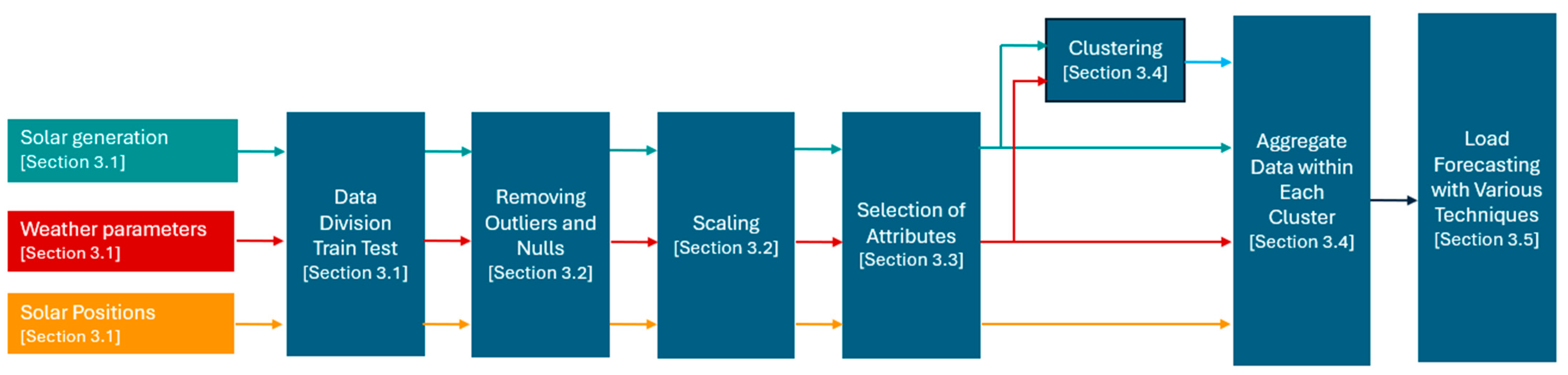
The research methodology began with obtaining raw utility data, removing outliers and null values, then processing the data to integrate them into a relational database. To ensure uniformity and precision in the data, the next step was to perform data scaling. Following data scaling, feature analysis and selection of attributes are conducted, serving as key elements of this methodology. Subsequently, K-means clustering was introduced to group the PV sites into different clusters and aggregate the data within each cluster. These preparatory steps laid the foundation to develop the forecasting models. Figure 1 shows the flowchart diagram for the overall methodology and the subsequent sections explain the approach.

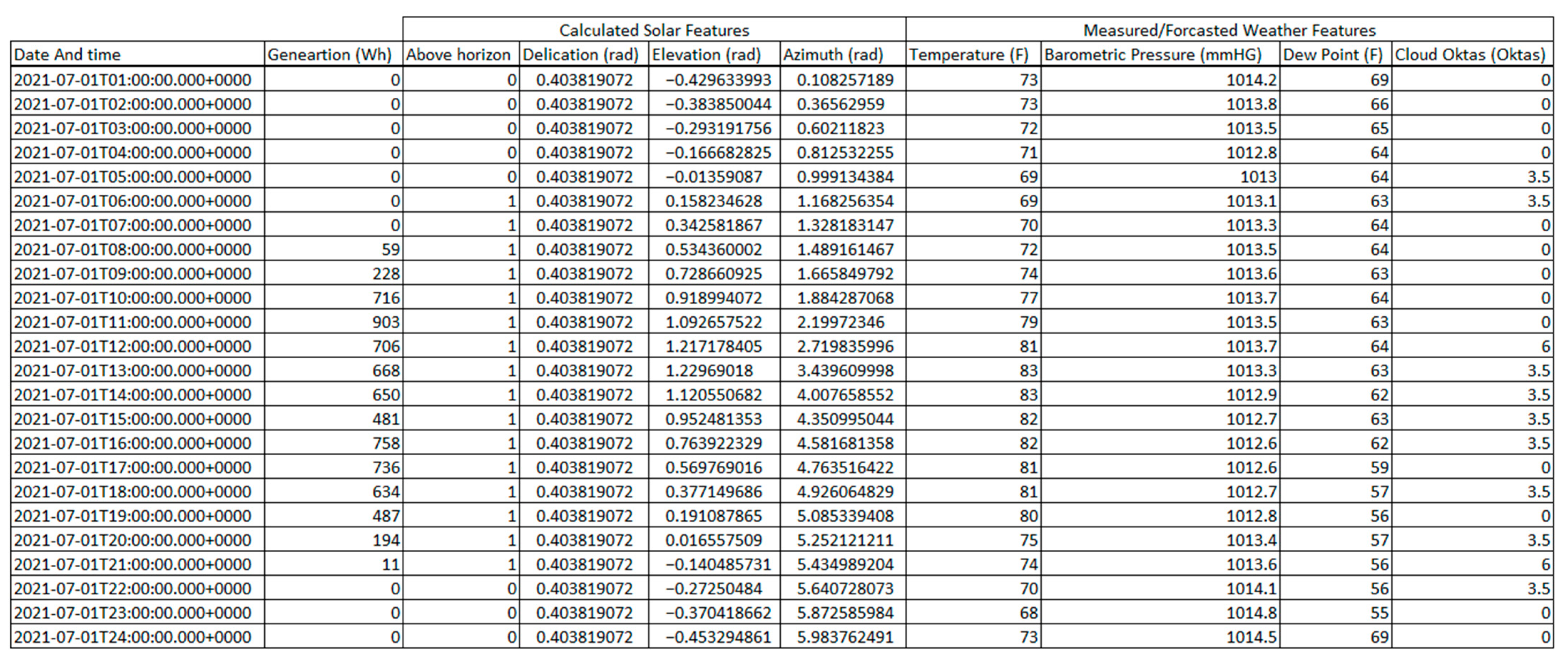
3.1. Data Collection

The historical hourly actual generation load data were obtained from an electric utility in Michigan. The utility provided weather information at hourly intervals from weather stations at 12 different local airports. The data covered a period of 24 months from January 2021 to December 2022, and included both the measured values and predicted values at horizons from 1 hour to 168 h. Data from 2021 were used to train the model (2021 training datasets) and data from 2022 were used as the test data (2022 testing datasets).

The weather parameters contained in the dataset were temperature (temp), barometric pressure (BP), dew point (dew), and cloud cover measured in oktas (oktas).

Using the Solar PV site latitude longitude coordinates and formulas provided by the National Oceanic and Atmospheric Administration calculator [40], the following features were calculated for each PV site at every hourly timestamp in the data to describe the sun’s position in the sky:

• Elevation angle in radians (elevation): This feature calculates the angle of the sun above the horizon, providing insights into the sun’s height in the sky.
• Declination angle in radians (declination): representing the angle between the rays of the sun and the plane of the Earth’s equator, this feature indicates solar declination.
• Azimuth angle in radians (azimuth): the azimuth angle signifies the sun’s compass direction, measured in radians, providing information about the sun’s position along the horizon.
• Boolean variable for sun’s visibility (above horizon): a binary variable (0 or 1) is employed to denote whether the sun is above the horizon during a specific timestamp.

The full unscaled dataset is not available to the public due to information security for the utility company’s customers; however, a sample of unscaled data is shown in Figure 2.

3.2. Data Processing and Scaling

In the process of refining the dataset, an approach was taken to handle outliers and missing values within the load generation and weather data.

Outliers within the load generation data were identified through the creation of box plots, both on a monthly and seasonal basis. This approach allowed for an understanding of load generation patterns across different timeframes. The outliers, once identified, were replaced using the backfill method. This method involves filling missing values with the most recent non-missing value, ensuring a continuous dataset.

Null values within the load generation data were addressed through a twofold process. Firstly, null values were entirely removed from the dataset, ensuring the integrity of the remaining data points. Secondly, the backfill method, which involves replacing the missing values at a given hour with the value from the next hour, was employed to impute missing values in the load generation data, presenting a consistent and logical replacement mechanism that aligns within the dataset.

For the weather data, null and missing values were inputted using information from the nearest weather station. This method ensured that the missing values were filled with relevant and applicable data from the closest available weather source. This approach preserved the accuracy of the weather data, providing a more comprehensive and consistent set of meteorological information for data analysis and forecasting.

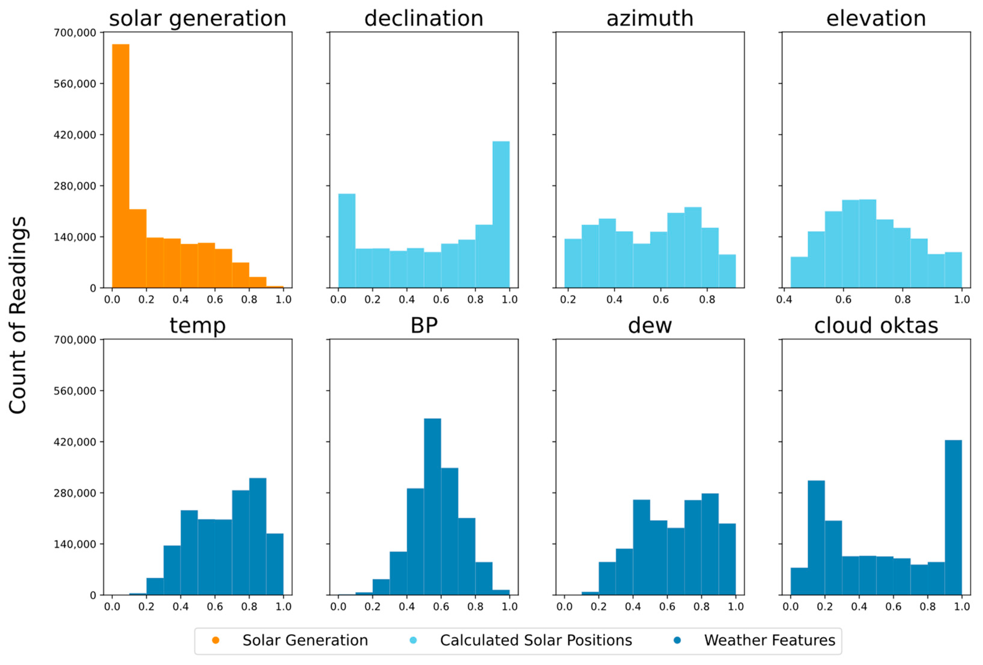
Next, each feature’s data underwent normalization through a min–max scaler, calibrated based on the 2021 training dataset. This normalization process was applied uniformly to both the 2021 training and 2022 testing datasets. In accordance with the utility company’s data security requirements, the target variable, representing load generation within the range of 5–15 MW, was also scaled to align within the 0 to 1 range. This scaling was performed using a min–max scaler fitted to the data from the 2021 training datasets and was consistently applied to both the 2021 training and 2022 testing datasets. A visual representation of the scaled distribution of features and the target variable is presented in Figure 3, where the x axis represents the data scaled between 0 and 1, and the y axis represents the count of readings for a certain scaled data (for example, count of readings for 0.5 scaled data for solar generation).

3.3. Feature Attributes Analysis and Selection

The accuracy of the weather forecast parameters was assessed by comparing measured values to predicted values at multiple time horizons: 24 h, 48 h, 72 h, 96 h, 120 h, 144 h, and 168 h.

Table 2. Mean absolute error percentage over various forecast horizons.

Weather Parameter	1 Day	2 Day	3 Day	4 Day	5 Day	6 Day	7 Day
Temperature (F)	2.0	2.4	2.7	3.3	4.1	4.1	4.2
BP (mmHG)	7.1	7.5	7.4	8.9	9.3	9.5	11.6
Dew Point (F)	1.6	2.3	2.6	3.9	5.1	5.3	5.8
Cloud Oktas (Oktas)	10.5	15.4	16	17.1	18.2	25.7	26.8

presents the mean absolute error percentage (10) for each scaled weather parameter across these different time horizons.

As each weather feature’s values were normalized to a scale between zero and one, this facilitated comprehensive comparisons of mean absolute errors across features. The temperature forecast exhibited the lowest error, with a mean absolute value ranging from 2% at 24 h to 4.2% at 168 h. Similarly, the dew point forecast demonstrated minimal error, ranging from 1.6% at 24 h to 5.8% at 168 h. However, the predicted values encountered challenges to accurately predict barometric pressure, resulting in a mean absolute value ranging from 7.1% at 24 h to 11.6% at 168 h. Cloud oktas displayed the highest mean absolute value, ranging from 10.5% at 24 h to 26.8% at 168 h. On the contrary, solar features, being directly calculable, exhibited negligible error in forecasting solar elevation, declination, and azimuth angles compared to the measured values.

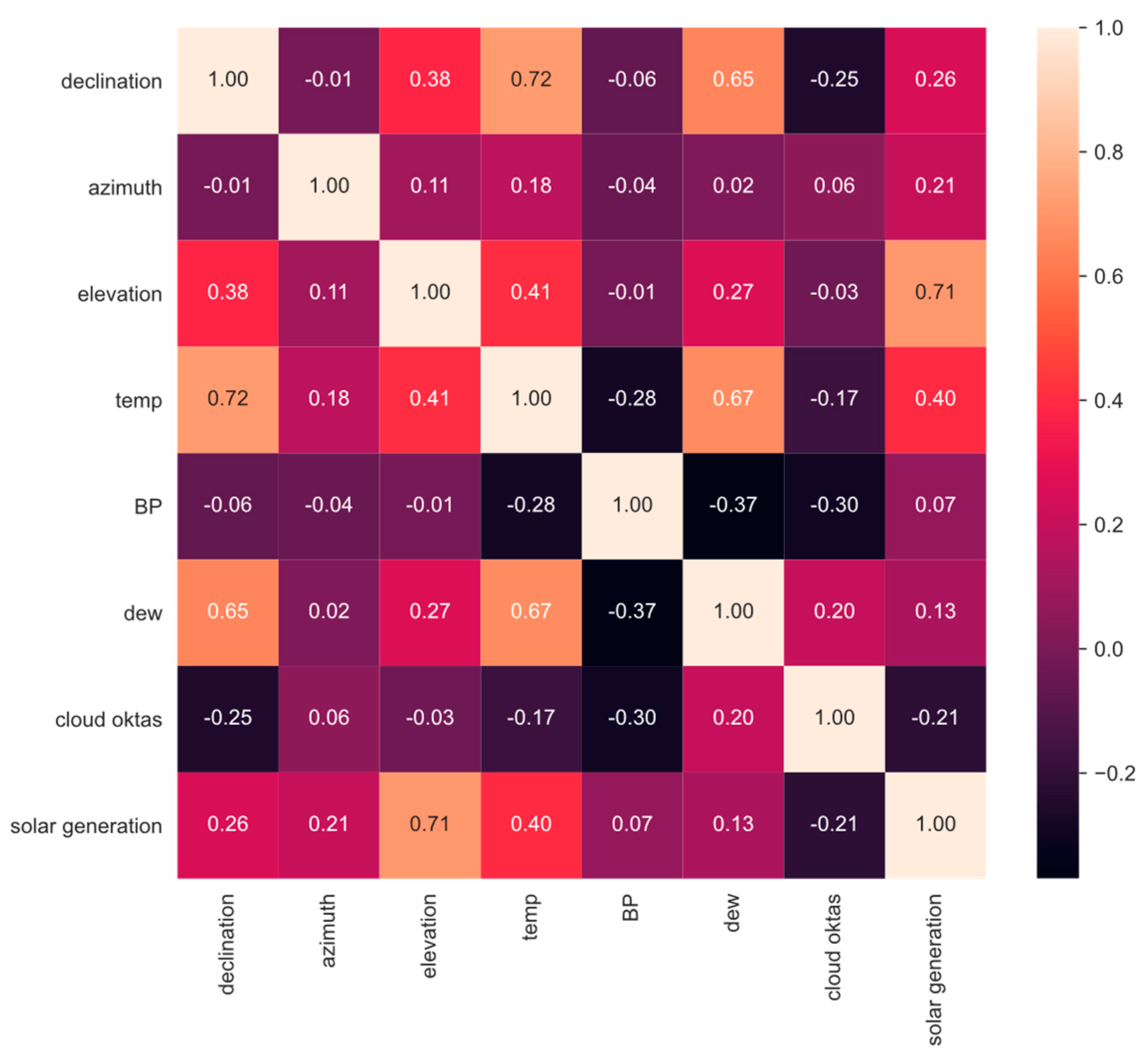
Next, Pearson correlation scores were computed between each feature variable and the target variable within the training dataset, as illustrated in Figure 4. Notably, solar elevation demonstrated the highest correlation to the target variable, registering a coefficient of 0.71. The other two solar features, namely, declination and azimuth angle, exhibited some correlation with the target variable, recording coefficients of 0.26 and 0.21, respectively. Among the measured weather features, the temperature variable displayed a moderate correlation to the target variable, with a coefficient of 0.4. In contrast, cloud oktas revealed a negative correlation score to solar generation of −0.21, indicating that cloud cover has a general effect of lower solar generation. On the other hand, barometric pressure and dew point did not exhibit significant correlations with solar generation, registering coefficients of 0.07 and 0.13, respectively.

Selection of attributes for the model was guided by the correlation scores with solar generation. The three solar features, along with temperature and cloud oktas, were chosen due to their notable correlation with solar generation. Although dew point and barometric pressure exhibited lower correlation with the target variable, they demonstrated significant correlations with cloud oktas. While correlation with other input features often suggests potential redundancy, incorporating these variables may contribute to mitigating errors in forecasted cloud oktas values, thereby enhancing model performance across extended forecast horizons. The analysis of this hypothesis is presented in Section 4. Therefore, dew point and barometric pressure were included as variables in the model.

3.4. K-Means Clustering

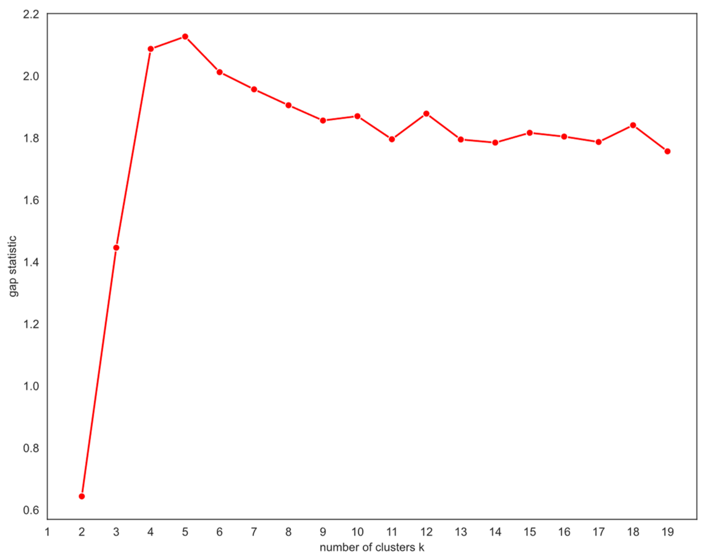
To improve the overall accuracy of the forecasting, a K-means clustering algorithm was used to group the PV sites into different clusters. Average historical solar load generation, along with average measured temperature, barometric pressure, dew point, and cloud cover from the 2021 training dataset, were used as features to group the customers. Since the dataset represents a small geographic area in southeast Michigan, the calculated solar positions did not show much variation at a given hour across the territory and were therefore excluded from the clustering analysis. Five clusters were selected as the optimum number using the gap statistic proposed in [41], which is computed using the following steps. First, the within cluster sum of squares (WCSS) metric is calculated for different number of clusters (k), which measures the distance from the centroid of a cluster to each member within that cluster. The resulting plot exhibits a non-convex shape, as depicted in Figure 5. Next, the WCSS metric is recalculated for various numbers of clusters (k) using uniformly distributed sets of points drawn randomly across the input feature space. The logarithm (log) of the WCSS from the solar load generation and measured weather features is shown by the “observed log(WCSS)” trendline and the WCSS value of the uniformly distributed points is represented by the “expected log(WCSS)” trendline; Figure 6 illustrates both trendlines. Finally, the gap between the observed log(WCSS) and expected log(WCSS) is computed by subtracting each value of k, as shown in Figure 7.

As illustrated in Figure 6, as the number of clusters (k) increases in the dataset comprising solar generation and measured weather features, the observed log(WCSS) value declines more rapidly than the expected log(WCSS) value for uniformly distributed points. This discrepancy is reflected in an upward slope of the gap statistic. The peak observed at k = 5 in Figure 7 denotes the last k value where the observed log(WCSS) decreased faster than the expected log(WCSS). Beyond this point, the reduction in observed log(WCSS) aligns closely with the reduction in expected log(WCSS) achieved by the uniform points, indicating that further splitting the data into additional clusters does not yield significant structural insights. The gap statistic transforms the non-convex problem evident in Figure 5 into a convex problem with a global maximum, as illustrated in Figure 7, providing a robust mathematical approach for determining the optimal number of clusters (k).

The number of PV sites within each cluster was as follows: 194 PV sites in the first cluster, 76 PV sites in the second cluster, 57 PV sites in the third cluster, 15 PV sites in the fourth cluster, and 3 PV sites in the fifth cluster. Generation from individual PV sites was aggregated within each of the five clusters, compressing the data into five signals and minimizing the effect of any remaining anomalies in generations values.

3.5. Forecasting Models

Several supervised learning models were created to predict solar generation. Each model was trained using features chosen from the 2021 training datasets, namely, the measured weather parameters, calculated solar positions, and K-means clustering assignments. Aggregated load within each cluster was used as the target variable when training each model. Models were tested using 2022 testing datasets, with predictions made using the measured weather parameters and again with forecasted weather parameters at the following forecast horizons: 24 h, 48 h, 72 h, 96 h, 120 h, 144 h, and 168 h. The models were trained on a cloud-computing platform utilizing 16 CPU cores running at 3.2 GHz each, with a total memory capacity of 112 GB. Training times ranged from 50 to 120 seconds.

A simple linear regression model (LR) (1) was created. The input features for the model were temperature, BP, dew, cloud oktas, declination, azimuth, elevation, above horizon, and cluster number. Linear regression is a widely used method for load forecasting; it is a simple and easy-to-use method. Linear regression assumes a linear relationship between the dependent variable (load) and the independent variable (such as time or weather data), which is appropriate for load forecasting as load tends to follow a consistent trend over time. In addition, linear regression is efficient and able to handle large datasets, making it a practical option for load forecasting.

$$y=b_0+b_1{x}_1+b_2{x}_2+\cdots +b_n{x}_n$$

(1)

where $y$ is the predicted value; $x_1$, $x_2$, …, $x_n$ are the independent variables (weather parameters, calculated solar positions, and K-means clustering assignments); $b_0$ is the intercept; and $b_1$, $b_2$, …, $b_n$ are the slopes.

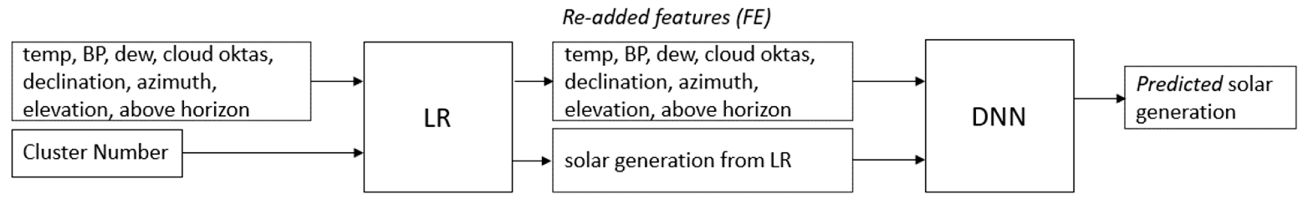
Next, two fully connected feedforward neural networks were used to predict solar generation; the models were LR+DNN and LR+FE+DNN.

Neural networks were preferred for short-term load forecasting due to their ability to model nonlinear relationships between variables, adapt to changes in load patterns, handle noisy and irregular data patterns, scale to large and complex datasets, and provide highly accurate forecasts.

The first model, LR+DNN, is represented in Figure 8 and can extend up to 168 hours. The input for the DNN was the solar generation from LR model.

The second model, LR+FE+DNN, also used the output of the linear regression model and re-added features (FE): temperature, BP, dew, cloud oktas, declination, azimuth, elevation, and above horizon as an input parameter to forecast solar generation. The model is represented in Figure 9 and can extend up to 168 hours. Each model used root-mean-square error and mean absolute error and full batch gradient descent to optimize the weights.

Each model used two hidden layers (2) within the rectifier linear unit (ReLU) function as the activation function between layers. A grid search was used to search for the optimum layer sizes.

The model was trained 5 times with different random starting states for each layer size option to ensure consistency of the results.

$$y=f_3(w_{32}·f_2(w_{21} · f_1(b_0+w_{11}\cdot x_1+w_{12}\cdot x_2+\cdots +w_{1n}\cdot x_n)+b_2)+b_3)$$

(2)

where $y$ is the forecasted generation value; $x_1$, $x_2$, …, $x_n$ are the independent variables (weather parameters, calculated solar positions, and K-means clustering assignments); $f_1$ and $f_2$ are the activation functions for the neurons in the first and second hidden layer; $w_{ij}$ are the weights between the input layer and the neurons in the first hidden layer; $w_{jk}$ are the weights between the neurons in the first and second hidden layers and $w_{kl}$ are the weights between the neurons in the second hidden layer and the output layer; $b_0, b_2, b_3$ are the bias terms. The network has two hidden layers, the first hidden layer with neurons labeled j and the second hidden layer with neurons labeled k.

Finally, long short-term memory (LSTM) model represented in Equations (3)–(9) was created to predict solar generation. LSTM is a type of neural network that is well-suited for handling sequence data and has been used for load forecasting due to its ability to capture long-term dependencies and temporal patterns in the data. LSTMs have a memory component that allows them to retain and use information from past observations in the sequence, which is useful for forecasting load, as load can be influenced by historical trends. Like other neural networks, LSTMs can model nonlinear relationships between variables, which is important in load forecasting as load can be influenced by various nonlinear factors such as weather conditions. The model is represented in equations below:

The data were processed using the forget gate, which determines whether the data should be retained or discarded. The function of the forget gate is obtained in Equation (3):

$$f_t=\mathsf{\sigma } \left( w_{if} · x_t+b_{if}+w_{hf}·h_{t-1}+b_{hf}\right)$$

(3)

where $f_t$ represent the forget gate, $\mathsf{\sigma }$ is the sigmoid expression, $w_{if}$ and $w_{hf}$ are the variable weights, $x_t$ is the sequence of the previous nine values at time t, $h_{t-1}$ is the previous output, and $b_{if}$ and $b_{hf}$ are the biases.

In the next phase, data are moved to the input gate represented in Equation (4):

$$i_t=\mathsf{\sigma } \left( w_{ii} · x_t+b_{ii}+w_{hi}·h_{t-1}+b_{hi}\right)$$

(4)

where $i_t$ denotes the activation of the input gate, controlling the amount of new information to be stored in the cell state; $w_{ii}$ and $w_{hi}$ are the variable weights; and $b_{if}$ and $b_{hf}$ are the biases.

Before the finale state, the results from the input gate are calculated using Equations (5) and (6); this is called cell state at time t:

$$g_t=\tan \mathrm{h} \left( w_{ig} · x_t+b_{ig}+w_{hg}·h_{t-1}+b_{hg}\right)$$

(5)

$$c_t=f_t · c_{t-1}+i_{t }· g_t$$

(6)

The output gate is represented in Equation (7). It determines what information from the cell state should be used to compute the hidden state (8), which is a combination of the cell state information (tanh ($c_t))$ and the output gate activation (${\mathrm{o}}_t)$:

$${\mathrm{o}}_t=\mathsf{\sigma } \left( w_{i\mathrm{o}} · x_t+b_{i\mathrm{o}}+w_{h\mathrm{o}}·h_{t-1}+b_{h\mathrm{o}}\right)$$

(7)

$${\mathrm{h}}_t={\mathrm{o}}_t · \tan \mathrm{h}\left(c_t\right)$$

(8)

The last step is to obtain the predicted value $y_t$ (9) by applying a transformation to the hidden state ${\mathrm{h}}_t$. Since the model is sequence to sequence, a dense layer was applied to each timestep of the sequence:

$${\mathrm{y}}_t=\mathrm{Dense}\left(h_t\right)$$

(9)

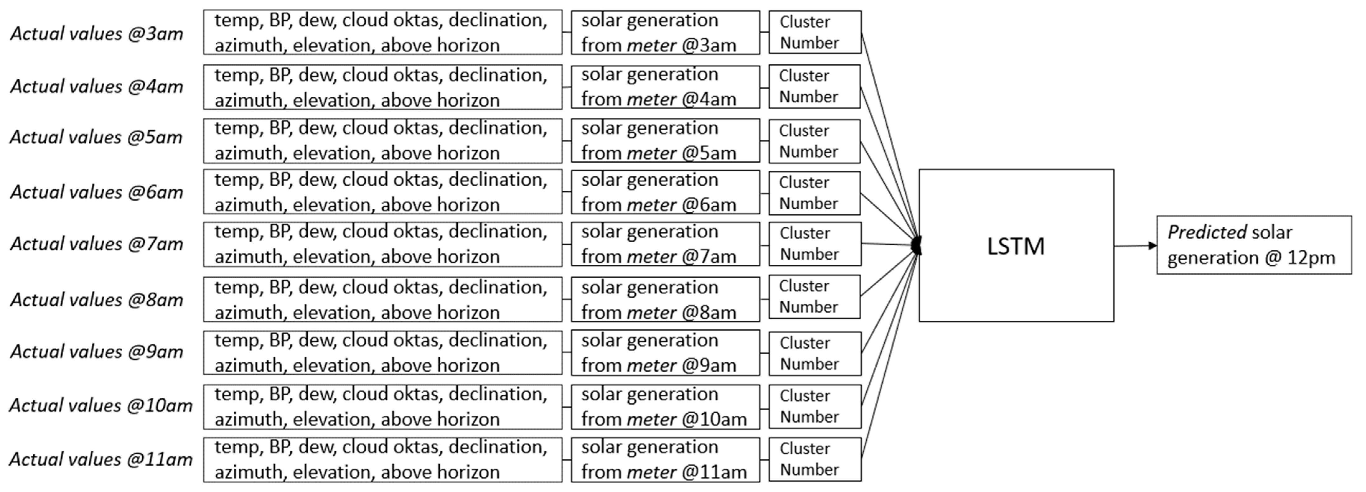
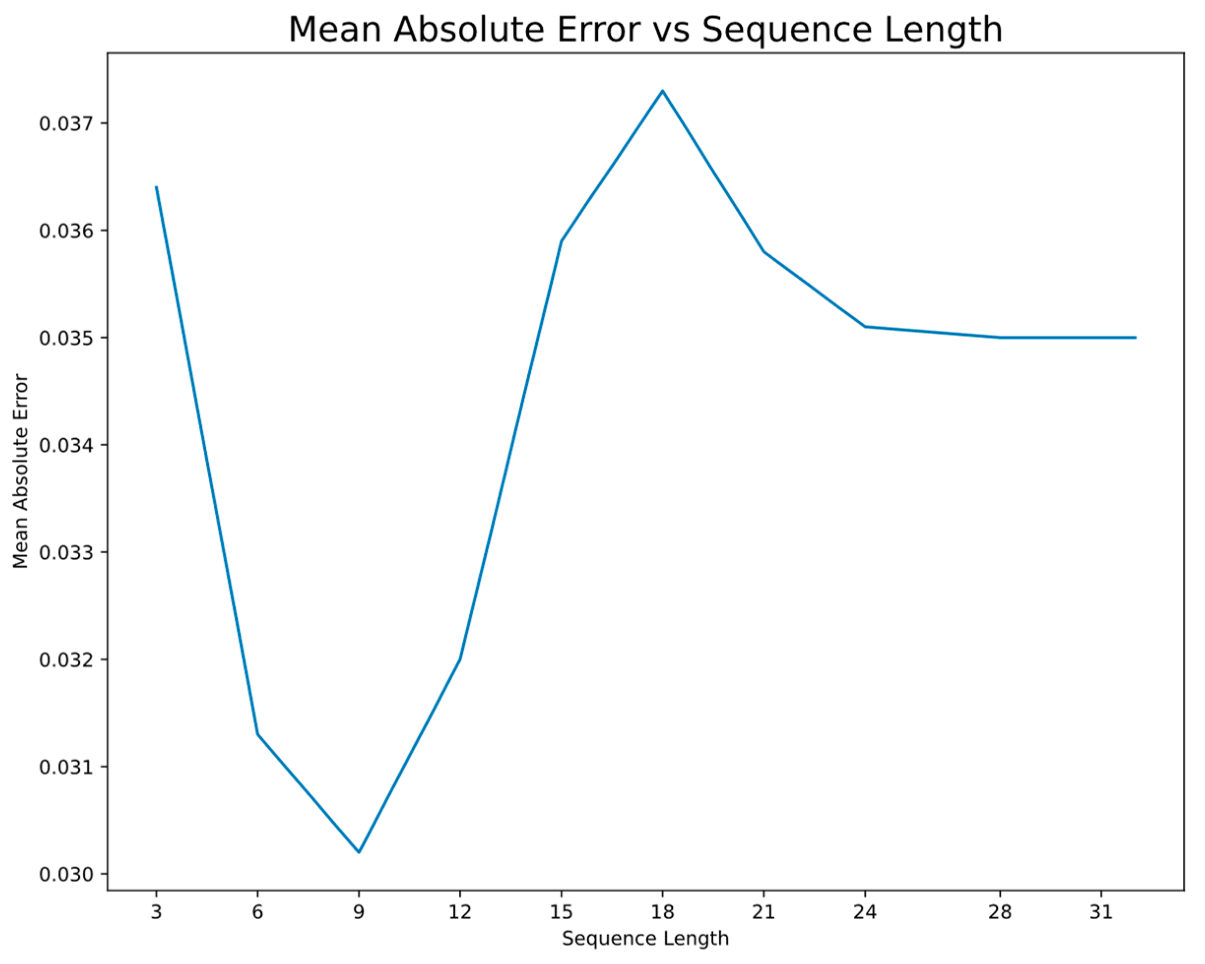
Sequential models such as LSTM look at the previous solar generation values, whether measured or forecasted, to predict the next most likely value in the future. The model was run in sequence to vector mode, where a sequence of the previous nine values were used to predict generation for one timestep into the future.

A sequence length of 9 was chosen by comparing the performance of various sequence length during a grid search. As shown in Figure 10, a sequence length of 9 achieved the lowest amount of mean absolute error.

The model has the capability to forecast up to 168 h. To illustrate this, to predict generation at 12 p.m., the model relies on a sequence of nine historical actual values from 3 a.m. to 11 a.m. The features are temp, BP, dew, cloud oktas, declination, azimuth, elevation, above horizon, actual solar generation from the meter, and cluster number. This process is visualized in Figure 11.

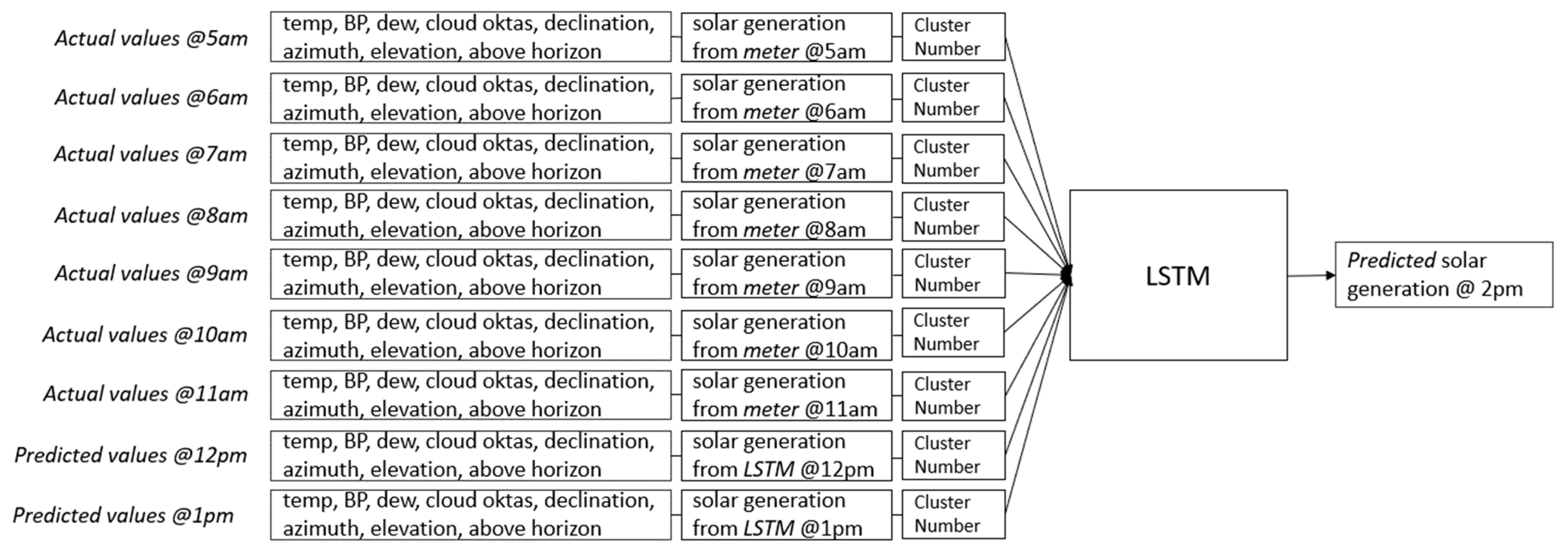
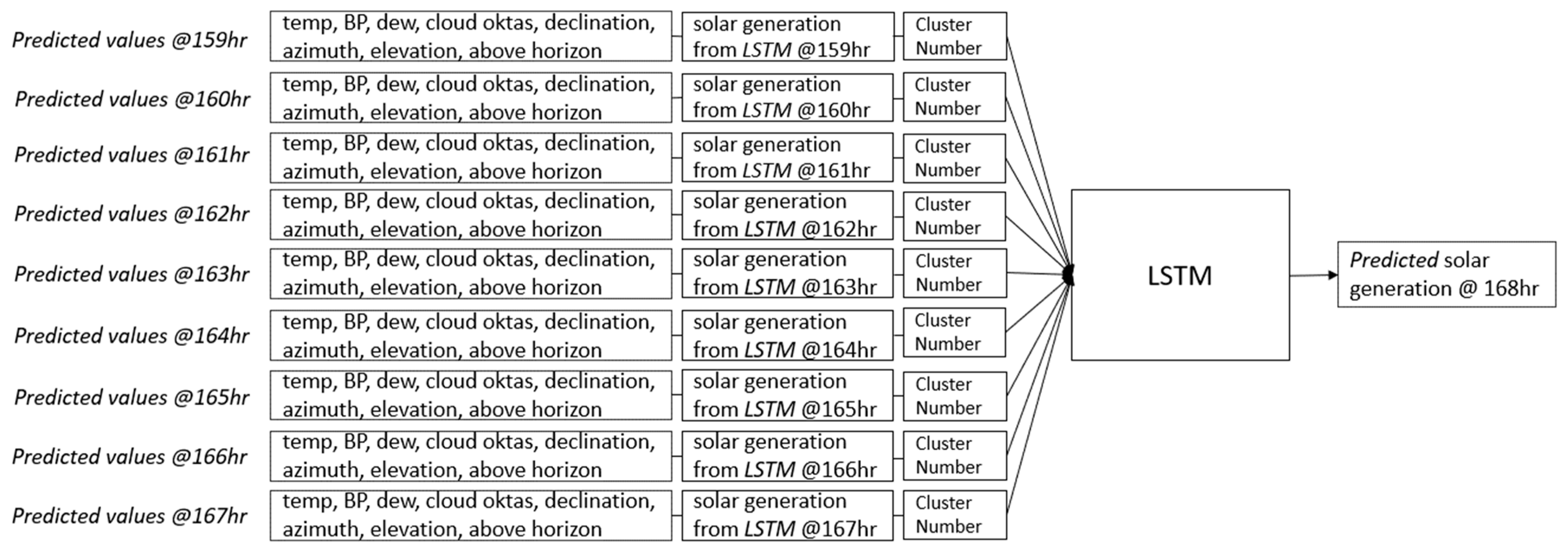
Similarly, to predict generation at 1 p.m., the hourly data window should span from 4 a.m. to 12 p.m., and the model employs a sequence of eight historical actual values from 4 a.m. to 11 a.m. for temp, BP, dew, cloud oktas, declination, azimuth, elevation, above horizon, actual solar generation from the meter, and the cluster number. In addition, there is one predicted value at 12 p.m. for temp, BP, dew, cloud oktas, declination, azimuth, elevation, above horizon, and actual solar generation from the LSTM model. This scenario is represented in Figure 12. Figure 13, Figure 14 and Figure 15 illustrate how the model predicts generation for subsequent hours. Note that the cluster number must stay the same for this scenario.

Mean absolute error (MAE), root-mean-square error (RMSE), mean absolute percentage error (MAPE), and coefficient of determination (R²) were used to evaluate the performance as the model used a single LSTM layer. The model was trained using full batch gradient descent. A grid search methodology, as described above, was used to choose the optimum LSTM layer and window size.

Benefits of Combining K-Means with LR, DNN, and LSTM

The primary benefit of a combined model lies in its ability to leverage the strengths of its component techniques, resulting in a more robust learning pattern. By addressing the weaknesses of individual methods, the combined model can improve overall accuracy and reinforce the respective advantages [42] of the component methods. Our model utilizes deep learning and LSTM, a cutting-edge machine learning technique that utilizes artificial neural networks and has recently emerged as an approach for solar power forecasting [22]; this particular form of deep learning has been validated and showcased as a highly effective model for tackling numerous complex learning tasks, including load forecasting [25].

4. Model Results and Evaluations

The utility currently uses PVWatts to calculate the forecasted generation load for their customers. PVWatts is a web application developed by the National Renewable Energy Laboratory (NREL). It allows homeowners, small building owners, installers, and manufacturers to easily develop estimates of the performance of potential PV installations [43]. The users can obtain the estimates by following a few steps: input the location, provide basic information about the PV system, and generate a results page that includes the estimates of the PV system’s load production. This information is often presented in terms of monthly or hourly and annual energy production figures measured in kilowatt-hours (kWh) [43]. The utility obtains forecasted data for individual customer locations through downloadable PDF or CSV files. Subsequently, it computes the discrepancy between the actual and the predicted generation loads, resulting in an MAE of 14.32%, an RMSE of 23.13%, an MAPE of 16.7%, and an R² of 0.58.

However, it is crucial to be aware of certain limitations inherent in its design. Firstly, the utility is constrained from utilizing its own comprehensive data files containing weather and generation data to execute the forecast [43]. Instead, the forecast process must be carried out individually for each location, following the description above. Secondly, the size estimator lacks the capability to discern roof angles and ground slopes. This omission is significant, as these factors play a crucial role in determining the actual efficiency of a solar system. Additionally, the tool does not incorporate shading analysis, overlooking potential obstructions like roof vents, structures, trees, or nearby objects that can impact solar panel performance.

Moreover, acknowledging uncertainties tied to weather data and the modeling approach, it is recognized that monthly estimated values may experience fluctuations within a range of approximately ±30%, and annual estimated values may exhibit variations of up to ±10% [43]. In addition, the tool assumes the use of modules with crystalline silicon or thin-film photovoltaic cells, potentially neglecting the considerations for other types of solar technologies [43].

While PVWatts offers a valuable starting point for assessing solar projects, recognizing its limitations emphasizes the importance of adopting a thorough and customized approach for accurate load forecasting. This recognition has fueled the motivation to develop a dedicated model that seamlessly integrates into the day-to-day operations of the utility.

The performance evaluation of the three models utilized in this study was conducted by analyzing their respective metrics using daytime values from the test dataset. Daytime values were exclusively used because the nighttime solar generation is virtually 0. Predicting the generation at night becomes a trivial task for the models, especially when solar positions are included in the features, and including nighttime readings artificially inflates the model performance statistics. Therefore, the test data were filtered to exclude nighttime readings using the calculated solar positions for the computation of all metrics shown in this research. The metrics used to evaluate the model’s performance were as follows:

• The mean absolute error (MAE) (10), which is a metric used to evaluate the accuracy of the models by measuring the average absolute differences between the predicted and actual values.
• The root-mean-square error (RMSE) (11), which emphasizes larger errors because it involves squaring the difference between actual and predicted values.
• The mean absolute percentage error (MAPE) (12), which computes the absolute percentage difference between each predicted value and its corresponding actual value, then averages these differences across all observations, and is expressed as a percentage.
• The coefficient of determination (R²) (13), which indicates the level of explained variability in the predicted values. A higher value indicates that a larger proportion of the variability in the observed load data is accounted for by the model, suggesting a better fit of the model to the data.

$$\mathrm{MAE}=\frac{1}{n}{{\displaystyle \sum }}_{i=1}^n\left|y_i-{\overline{y}}_i\right|$$

(10)

$$\mathrm{RMSE}=\sqrt{\frac{1}{n}{{\displaystyle \sum }}_{i=1}^n{\left(y_i-{\overline{y}}_i\right)}^2}$$

(11)

$$\mathrm{MAPE}=\frac{1}{n}\ast {{\displaystyle \sum }}_{i=1}^n\left|\frac{y_i-{\overline{y}}_i}{y_i}\right|\times 100\%$$

(12)

$$R^2=1-\frac{{{\displaystyle \sum }}_{i=1}^n{\left(y_i-{\overline{y}}_i\right)}^2}{{{\displaystyle \sum }}_{i=1}^n{\left(y_i-\mu \right)}^2}$$

(13)

where n is the number of observations, $y_i$ represents the actual values, ${\overline{y}}_i$ represents the predicted values, and $\mu$ is the mean of the actual values. Since the aggregated generation within each cluster was scaled to fall between zero and one, as described in Section 3.2, each error metric is in scaled generation units and represents the total error across all five generation clusters. To calculate the MAE and RMSE in percentage terms, we divided each respective error metric (obtained from (10) and (11)) by the mean of the actual values and then multiplied the result by 100.

The results are presented in

Table 3. Daytime performance metrics evaluation using measured weather values.

Models	MAE	RMSE	MAPE	R2
Utility Baseline	14.32%	23.13%	16.7%	0.58
LR+DNN	9.12%	13.22%	9.88%	0.79
LR+FE+DNN	5.97%	9.18%	6.43%	0.9
LSTM	5.7%	8.79%	5.91%	0.93

. The model’s results were compared with the baseline model provided by the utility, which represents their existing model.

The “Utility Baseline” served as a benchmark against which the performance of the subsequent models was compared. It achieved MAE, RMSE, MAPE, and R² values of 14.32%, 23.13%, 16.7%, and 0.58%, respectively. These metrics indicate that the Utility Baseline model provides an uncertain level of accuracy in predicting solar load generation, which implies that there is significant room for improvement.

The first model developed was the “LR+DNN” model, which combines linear regression (LR) with a deep neural network (DNN). We observed notable improvements across all performance metrics. With lower MAE, RMSE, and MAPE values of 9.12%, 13.22%, 9.88%, respectively, and a higher R² value of 0.79%. The LR+DNN model demonstrated enhanced accuracy and precision compared to the baseline model. This suggests that the incorporation of the DNN architecture complemented the LR model, resulting in more accurate and reliable predictions of solar load generation.

Furthermore, the “LR+FE+DNN” model exhibited even greater improvements in performance metrics. With MAE, RMSE, MAPE, and R² values of 5.97%, 9.18%, 6.43%, and 0.9%, respectively, this model achieved a higher accuracy and precision compared to both the baseline and LR+DNN models. Re-adding the features (FE) likely contributed to the extraction of more informative features, thereby enhancing the predictive capabilities of the model.

Lastly, the “LSTM” model, which utilizes long short-term memory neural networks, demonstrated the highest level of performance among all models. With the lowest MAE, RMSE, and MAPE values of 5.7%, 8.79%, 5.91%, respectively, and the highest R² value of 0.93%, the LSTM model outperformed all other models in terms of accuracy and precision. LSTM’s ability to capture long-term dependencies in sequential data likely contributes to its superior forecasting capabilities in solar load generation. Additionally, its performance appears to be particularly robust when handling extreme values within the dataset, indicating a high level of reliability and accuracy even in challenging scenarios.

In summary, the evaluation of performance metrics highlighted the incremental improvements achieved by each successive model in predicting solar load generation. From the baseline model to the LSTM model, there was a clear trend of enhanced accuracy, precision, and overall performance, underscoring the importance of incorporating sophisticated modeling techniques in solar load forecasting applications.

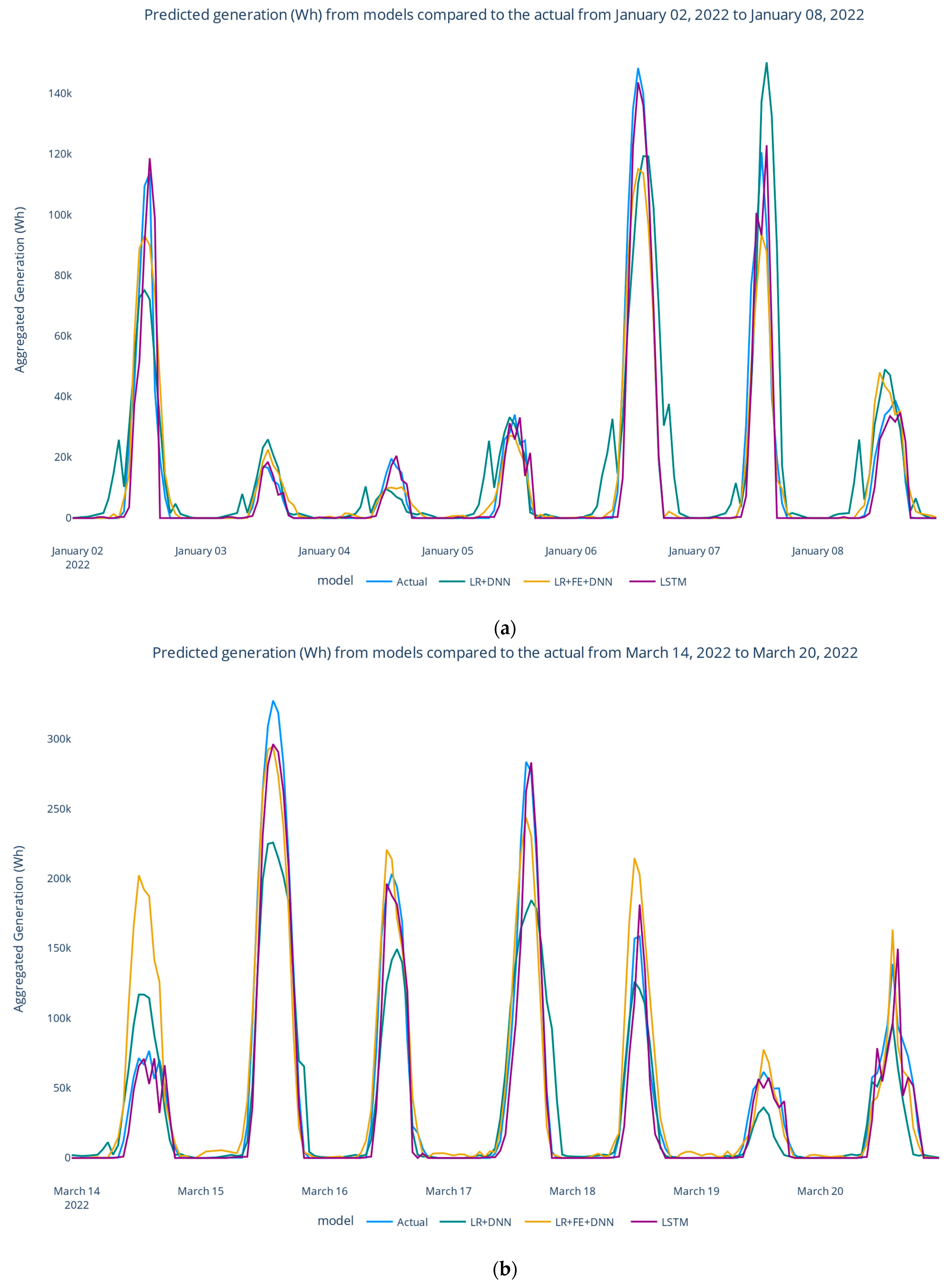
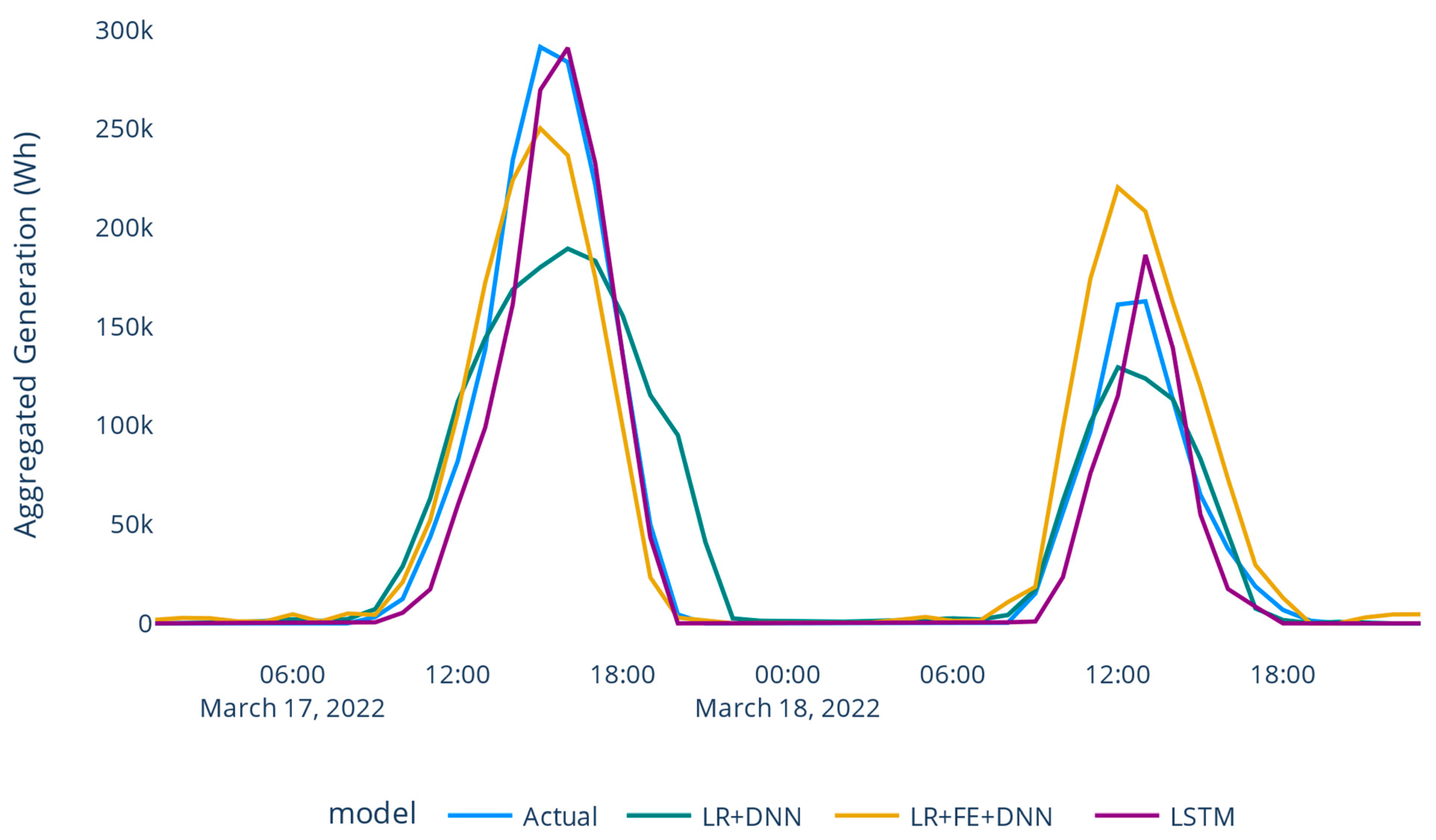
The forecast generation is shown in Figure 16, where (a) shows 168 h in the winter, (b) spring, (c) summer, and (d) fall. Figure 17 provides a detailed view for one day of the predicted solar load generation across all models, while Figure 18 displays it spanning two days. Notably, from Table 3 and Figure 16a–d, the LSTM model, which yielded the lowest performance metrics, closely approximated the actual peak generation values compared with the alternative model. Moreover, the model achieved a better prediction when there was a change in the actual generation load from one day to another, as shown in Figure 16a–d.

For example, on 24 October, the actual load was around 180 KWh (peak); however, the next day, the actual load changed and dropped to 60 KWh (peak). The LSTM model (purple) performed much better than the LR+FE+DNN model (yellow). The LSTM model was much closer to the actual load than the LR+FE+DNN model.

Based on these observations, it can be concluded that the LSTM model outperformed the other two models in terms of predictive accuracy and reliability.

Overall, the findings highlight the favorable performance of the LSTM model and its potential for effectively forecasting the generation load.

The evaluation of the LR+FE+DNN model unveiled a noteworthy concern regarding its tendency to overpredict the generation load, particularly in scenarios involving daily fluctuations in the actual load generation. This persistent overprediction phenomenon indicates that the model consistently projected values that exceeded the true load values. Such a pattern can have adverse effects, including inefficient resource allocation and operational inefficiencies.

In contrast, the LSTM model demonstrated a superior capability to address this issue and offer more accurate load predictions. Leveraging its ability to capture long-term dependencies and effectively handle sequential data, the LSTM model proved adept at capturing and adapting to the daily changes in actual load generation.

The visual representations in Figure 16, Figure 17 and Figure 18, showcase the remarkable proximity of the LSTM model’s forecasted outputs to the actual peak generation levels, serving as evidence of its enhanced accuracy in predicting load variations. By successfully capturing the underlying patterns and dynamics of the data, the LSTM model effectively tackled the challenges posed by daily fluctuations, resulting in predictions that closely aligned with the true values.

The significance of avoiding overprediction of generation load lies in its practical implications. Overestimating the load demand can lead to undesired outcomes, such as excessive resource allocation, unnecessary costs, and potential strain on the power grid. By effectively mitigating the overprediction issue, the LSTM model showcased its ability to deliver more reliable and precise load forecasts. This will enable utilities to optimize resource allocation, enhance operational efficiency, and maintain a stable and resilient power system.

To establish a benchmark, similar models to the previous research methods in Table 1 were implemented and run on the same data. Specifically, we deployed a gradient boosted tree similar to the one in [31], a Gaussian process regression similar to [37], and a support vector regression model resembling [36]. The autoregressive approaches outlined in [32] and [38] were omitted, as they traditionally operate on univariate data and did not readily confirm to bivariate data. The SOM approach from [35] posed a challenge for implementation based solely on the description in the published article, and hence was not included. The NN ensemble [39] was also excluded due to its reliance on neural network models. The specific features used by each author were not available in the utility dataset, so instead each algorithm was trained using the calculated solar and measured weather data from the 2021 training datasets, and was then evaluated on the 2022 testing datasets. A comparison of the performance metrics across a seven-day forecasting horizon is shown in

Table 4. Model performance metrics: daytime MAE percentage comparison over a seven-day forecast horizon.

Model Family	Model	Actual	1 Day	2 Day	3 Day	4 Day	5 Day	6 Day	7 Day
Support Vector Machine	SVR	7.7	8.2	8.5	8.9	9.3	9.9	10.6	10.9
Probabilistic	GPR	12.6	12.8	13.1	13.2	13.3	13.8	14	14.2
Gradient Boosted Tree	GBT	7.1	7.5	7.8	8.2	8.7	9.6	10.3	10.4
Neural Net (this article)	LR+DNN	9.1	9.8	10.1	10.4	10.8	11.4	11.9	12.1
	LR+FE+DNN	6	6.6	6.9	7.4	8	8.7	9.4	9.6
	LSTM	5.7	6.2	6.4	7	7.5	8.4	9.4	9.5

for the mean absolute error (MAE) and

Table 5. Model performance metrics: daytime RMSE percentage comparison over a seven-day forecast horizon.

Model Family	Model	Actual	1 Day	2 Day	3 Day	4 Day	5 Day	6 Day	7 Day
Support Vector Machine	SVR	10.2	10.8	11.3	11.8	12.7	13.9	15	15.4
Probabilistic	GPR	20.1	22.2	22.5	24	23.8	24.7	26.9	27.6
Gradient Boosted Tree	GBT	10.1	10.8	11.2	11.8	12.4	13.3	14.5	14.8
Neural Net (this article)	LR+DNN	13.2	14	14.5	14.8	15.4	16	16.9	17.2
	LR+FE+DNN	9.2	9.9	10.2	11.1	12	13.2	14.5	15
	LSTM	8.79	9.7	10.2	10.9	11.7	12.8	14	14.4

for the root-mean-square error (RMSE).

In this comparative analysis of various models for forecasting the solar generation load, the mean absolute error (MAE) values from Table 4 and root-mean-square error (RMSE) values from Table 5 were employed as key metrics to evaluate the performance across different forecast horizons.

The support vector machine (SVR) demonstrated a competitive performance with MAE values ranging from 7.7% to 10.9% and RMSE values ranging from 10.2% to 15.4%, providing reasonable accuracy but being outperformed by the other models in certain forecast horizons. The Gaussian process regression (GPR) exhibited the worst forecast accuracy, with MAE values ranging between 12.6% and 14.2%, and RMSE values between 20.1% and 27.6%. The gradient boosted tree (GBT) emerged as a strong performer with consistently low MAE values, ranging from 7.1% to 10.4%, and low RMSE values ranging from 10.1% to 14.8%. This model consistently demonstrated robust performance across various forecast horizons, making it one of the top-performing models.

Within the neural network family, three models were considered from this article: LR+DNN, LR+FE+DNN, and LSTM. LR+DNN and LR+FE+DNN exhibited competitive results, with MAE values ranging from 6% to 9.6% and RMSE values ranging from 9.2% to 15%. While these models showcased good accuracy, their performance was surpassed by LSTM in most cases. LSTM consistently outperformed the other models, achieving the lowest MAE values across all forecast horizons, ranging from 5.7% to 9.5%, and the lowest RMSE values across all forecast horizons, ranging from 8.79% to 14.4%. This highlights LSTM as the most accurate model for solar generation load forecasting in this comparison.

In summary, the detailed MAE and RMSE comparison underscored LSTM as the standout model, consistently providing the most accurate predictions across different forecast horizons. The results suggest the superiority of LSTM in capturing the complex patterns and dependencies inherent in solar generation data. This is likely due to the fact that our method combines the advantages of K-means clustering and LSTM networks. K-means clustering can identify patterns in solar power generation data, while the LSTM model is able to determine the temporal relationships between the data [44].

To assess the performance of LSTM across various weather conditions, three typical weather types were selected for comparison. These conditions were evaluated alongside models developed from previous research methods, as detailed in Table 1. The models were run on the same dataset to provide a thorough assessment of their performance.

Table 6. Daytime MAE percentage forecasting performance comparison under different seasons and weather types.

Season	Weather Types	SVR	GPR	GBT	LR+DNN	LR+FE+DNN	LSTM
Winter	Sunny	12.1	19.3	10.2	13.4	10.2	9.1
	Cloudy	7.9	9.8	7.5	7	6.7	6.3
	Rainy	7.3	8.3	6.1	5.4	4.3	4.1
Spring	Sunny	7.8	13.8	6.5	12.7	5.1	3.5
	Cloudy	9.5	17	10.1	12.1	8.9	9.8
	Rainy	8.2	19	8	10.2	7.6	7.3
Summer	Sunny	6.4	8.7	4.2	7.6	3.7	2.9
	Cloudy	7.8	7.5	7.8	7.4	6.5	6.3
	Rainy	9.5	12.3	10	10.2	8.6	8.9
Autumn	Sunny	9.8	17.9	7.3	14.4	8.2	5.5
	Cloudy	6.8	10.6	6.2	9	6.2	5.5
	Rainy	6	19.1	5.1	7.5	5.6	4.1

presents the results using MAE, while

Table 7. Daytime RMSE percentage forecasting performance comparison under different seasons and weather types.

Season	Weather Types	SVR	GPR	GBT	LR+DNN	LR+FE+DNN	LSTM
Winter	Sunny	15.4	32	14.1	18.8	14.8	13.4
	Cloudy	10.6	15.7	11	10.8	10.4	9.5
	Rainy	9.2	15.5	8.9	8.5	7.6	7
Spring	Sunny	9.6	21.9	9.3	16.8	7.1	5.9
	Cloudy	12.8	27.9	14.5	16.6	13	15
	Rainy	10.8	32.2	11.6	14.2	11	11.3
Summer	Sunny	8	14.5	6.2	10.4	5.7	5.1
	Cloudy	10.1	10.3	10.7	10.5	9.5	9.3
	Rainy	12.5	17.6	13.6	14.3	13.4	12.5
Autumn	Sunny	12	27.2	9.6	18.4	10.6	7.8
	Cloudy	8.9	15.4	8.7	13.1	9.5	8.4
	Rainy	7.8	48.5	7.3	11.5	9.4	6.8

displays the results using RMSE.

In the winter season, LSTM and LR+FE+DNN consistently demonstrated superior performance in terms of both the MAE and the RMSE, with LSTM excelling in sunny conditions and LR+FE+DNN exhibiting an almost similar accuracy to LSTM in cloudy and rainy conditions. LR+DNN and GBT consistently performed competitively across the weather types.

In spring, LSTM and LR+FE+DNN maintained a robust performance in terms of both the MAE and the RMSE, with LSTM standing out in sunny conditions. LR+FE+DNN and GBT showed notable accuracy in rainy conditions.

In the summer season, LSTM and LR+FE+DNN continued to lead in performance in terms of both the MAE and the RMSE, with LSTM displaying outstanding accuracy in sunny conditions. GBT performed well in sunny and cloudy conditions, while LR+FE+DNN demonstrated a competitive performance across the weather types.

In autumn, LSTM remained a consistent performer in terms of both the MAE and the RMSE, excelling in all weather conditions. GBT exhibited competitive accuracy, particularly in cloudy and rainy conditions.

This comprehensive comparison underscored the consistent superiority of GBT and LSTM across different seasons and weather types, with LSTM often emerging as the top-performing model in various conditions. These findings emphasize the robustness of these models in solar generation load forecasting.

Lastly, the permutation feature importance technique was used to evaluate how the model used each feature. Each model was run against the test set with one of the feature’s values randomly rearranged. If the model’s error increased using the permutated data, it indicated that the model was making use of that feature to generate its predictions. Conversely, if the error stayed approximately the same with the permutated data, it indicates the model was not using that feature. This process was repeated with five random permutations for each feature. The average increase in mean daytime error after permutating each of the calculated solar and measured weather values is shown in

Table 8. Daytime MAE increase after application of permutation feature importance.

Model Family	Model	Azimuth	Declination	Elevation	BP	Dew	Temp	Cloud Oktas
Support Vector Machine	SVR	0.038	0.013	0.128	0.000	0.068	0.073	0.037
Probabilistic	GPR	0.092	0.406	0.190	0.033	0.150	0.342	0.116
Gradient Boosted Tree	GBT	0.059	0.018	0.124	0.001	0.026	0.022	0.057
Neural Net (this article)	LR+DNN	0.001	0.023	0.078	0.000	0.138	0.214	0.001
	LR+FE+DNN	0.056	0.021	0.150	0.000	0.045	0.059	0.042
	LSTM	0.069	0.002	0.123	0.000	0.011	0.009	0.067

.

As indicated in Table 8, the observed increase in MAE post-permutation highlights that the LSTM model predominantly leveraged the azimuth, elevation, and cloud oktas features. The LR+FE+DNN model, which achieved the second-best performance in terms of error metrics, demonstrated a significant reliance on azimuth and elevation features. Interestingly, the model also exhibited a noticeable dependance on the dew feature, in conjunction with the cloud oktas feature, supporting the hypothesis presented in Section 3.3.

This hypothesis suggested that the models could capitalize on correlated features, such as dew or barometric pressure, to compensate for errors in forecasted cloud oktas. This discovery suggests a potential topic for further research, to investigate the advantages of leveraging correlated features in scenarios where feature values are forecasted and may contain an error.

5. Conclusions and Future Work

The research conducted in this study is intended for electric utilities. It utilized its load generation, AMI, and weather data to forecast the generation load using three different machine learning methods: linear regression with deep neural networks (LR+DNN), linear regression with features and deep neural networks (LR+FE+DNN), and long short-term memory (LSTM) forecasting. The results were compared using MAE and RMSE values, which were presented in Table 3, Table 4 and Table 5. Additionally, the performance was analyzed across various different seasons and weather types, as illustrated in Table 6 and Table 7.

This research revealed the indispensable role of weather features in achieving precise forecasts for the generation load. Considering the substantial variations in weather patterns across different seasons, accounting for these features proved critical for accurate predictions. Among the models assessed, the LR+FE+DNN model emerged as an effective solution in generating highly accurate predictions for the generation load, exhibiting minimal error. However, this model tended to over-forecast when weather changes caused the generation to increase or decrease from one day to the next. On the other hand, the LSTM model was able to solve this problem with great accuracy and precision, resulting in the lowest MAE and RMSE scores. The models were benchmarked against various models from different articles using same dataset. The LSTM model stood out for its demonstrated accuracy, consistency, and robust performance across different forecast horizons and weather types. Despite its notable achievements, the proposed LSTM model requires a large amount of training data to effectively learn complex patterns and dependencies within sequential data. Moreover, the efficacy of the proposed methodology hinges upon the availability of data from the utility; it is imperative that data covering at least six months are accessible. Without such a dataset, the LSTM may encounter challenges in terms of generalization and become susceptible to overfitting. Electric utilities typically have access to a wealth of data including historical consumption and generations patterns, weather data, and grid infrastructure information. However, ensuring the quality, consistency, and accessibility of these data is crucial for the success of the forecasting model. As for the regulatory requirements, electric utilities operate within regulatory frameworks that govern aspects such as data privacy (to ensure customer privacy, data related to customers’ must be scaled, following regulatory requirements). In addition, to address the computational requirements, cloud computing resources should be considered, which offer scalable infrastructure and services tailored for machine learning tasks.

The success of these models opens possibilities for future work, such as implementing hybrid models that combine LSTM with other machine learning techniques, for example, support vector machines (SVMs) or convolutional neural networks (CNNs), to improve the predicting accuracy. These hybrid approaches could leverage the strengths of different models to better capture the underlying patterns in solar generation data. Another area for future research involves monitoring solar locations and spotting unusual event behaviors by analyzing the differences between actual solar load generation and predicted data. This can be achieved through the development of techniques that quantify the deviations between the two datasets, facilitating the detection of unusual events or discrepancies in solar energy production. Additionally, the presented techniques can be applied to forecast the load of wind power generation. Overall, the findings suggest that incorporating weather data and using advanced machine learning techniques, such as LSTM, can significantly improve the accuracy and precision of generation load forecasting in the electric utility industry.