

Computational Fluid Dynamics Simulation of Filling a Hydrogen Type 3 Tank at a Constant Mass Flow Rate

 , , ,
, , ,  and
and 
Abstract
1. Introduction
2. CFD Simulations
2.1. Cases Studied
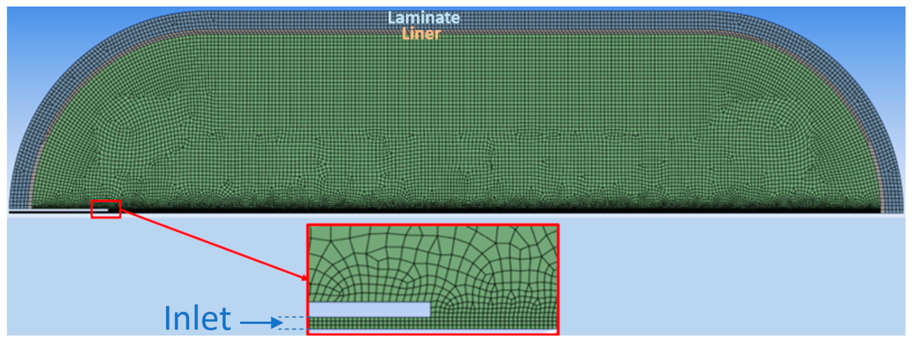
2.2. Preprocessing Settings
2.3. Governing Equations and Solver Settings
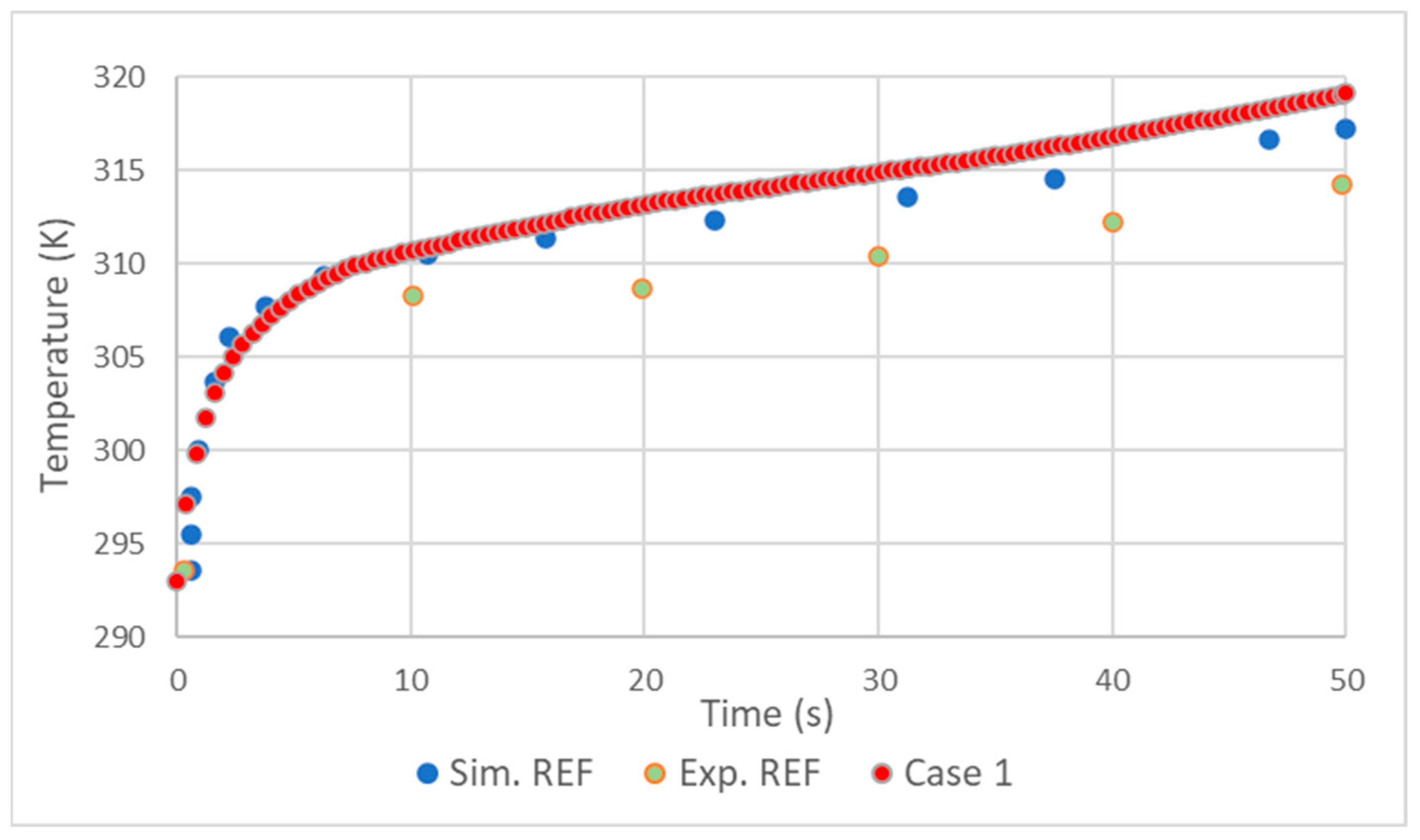
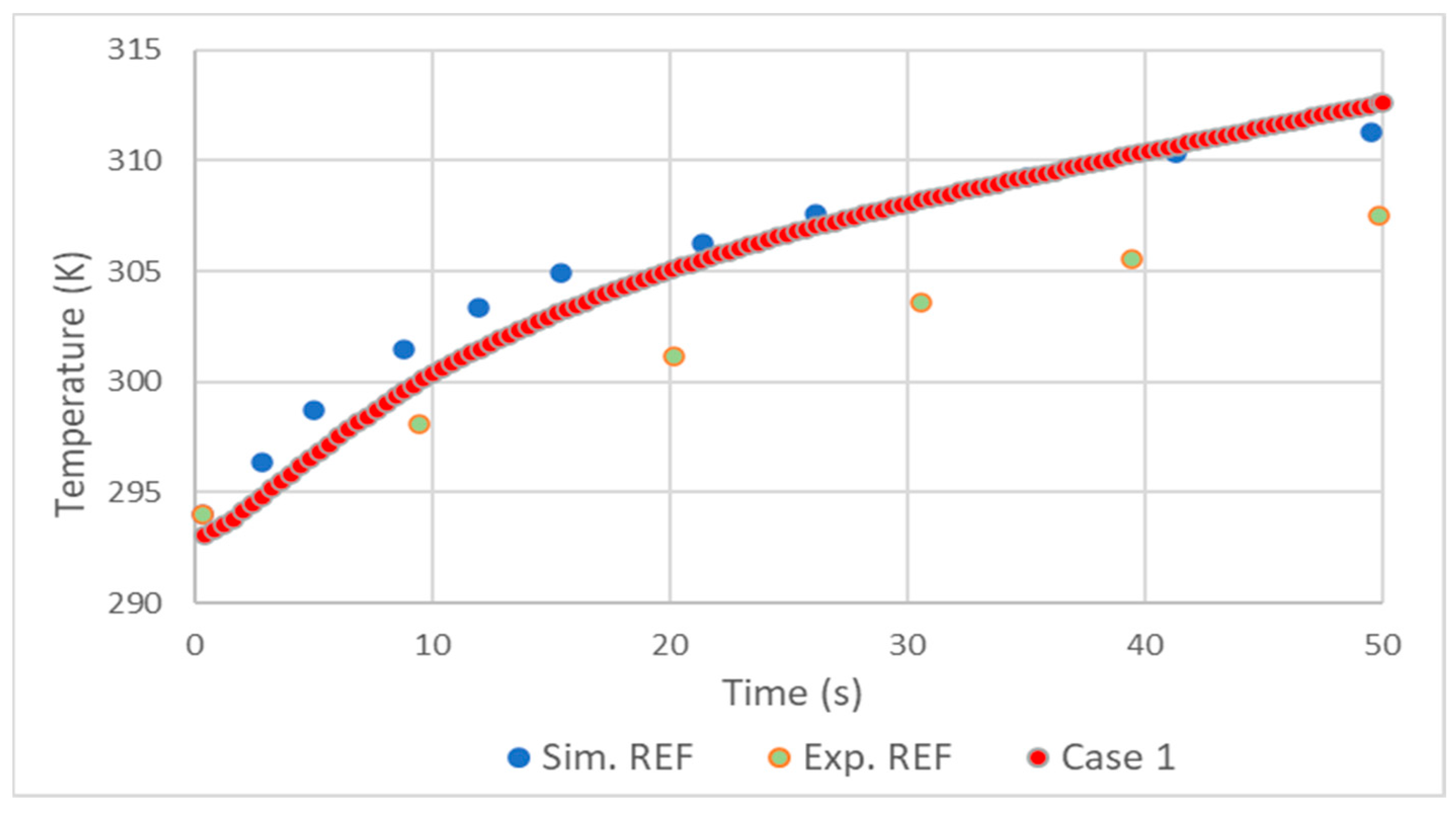
2.4. Validation
3. Results
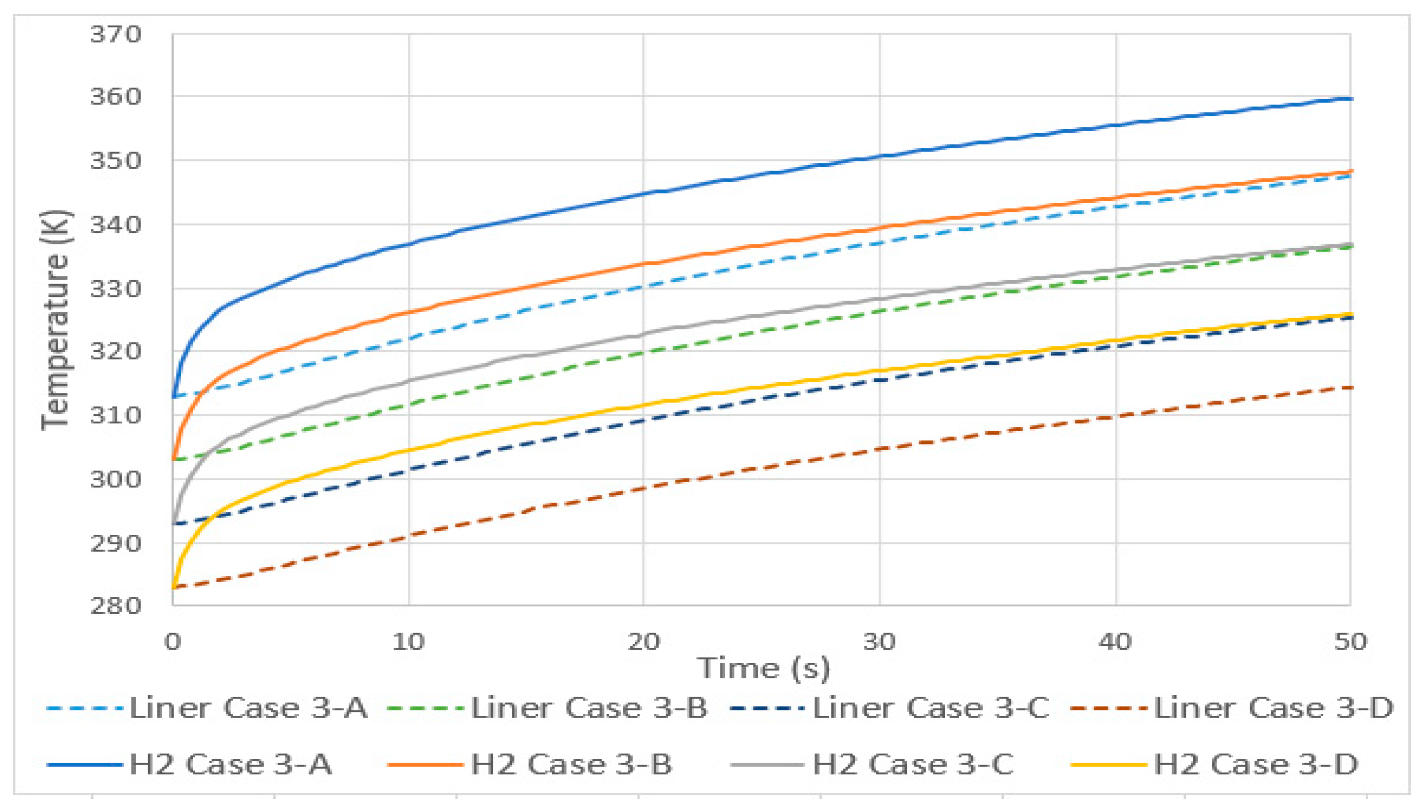
3.1. Increase in Temperatures in Total Equilibrium with Environment
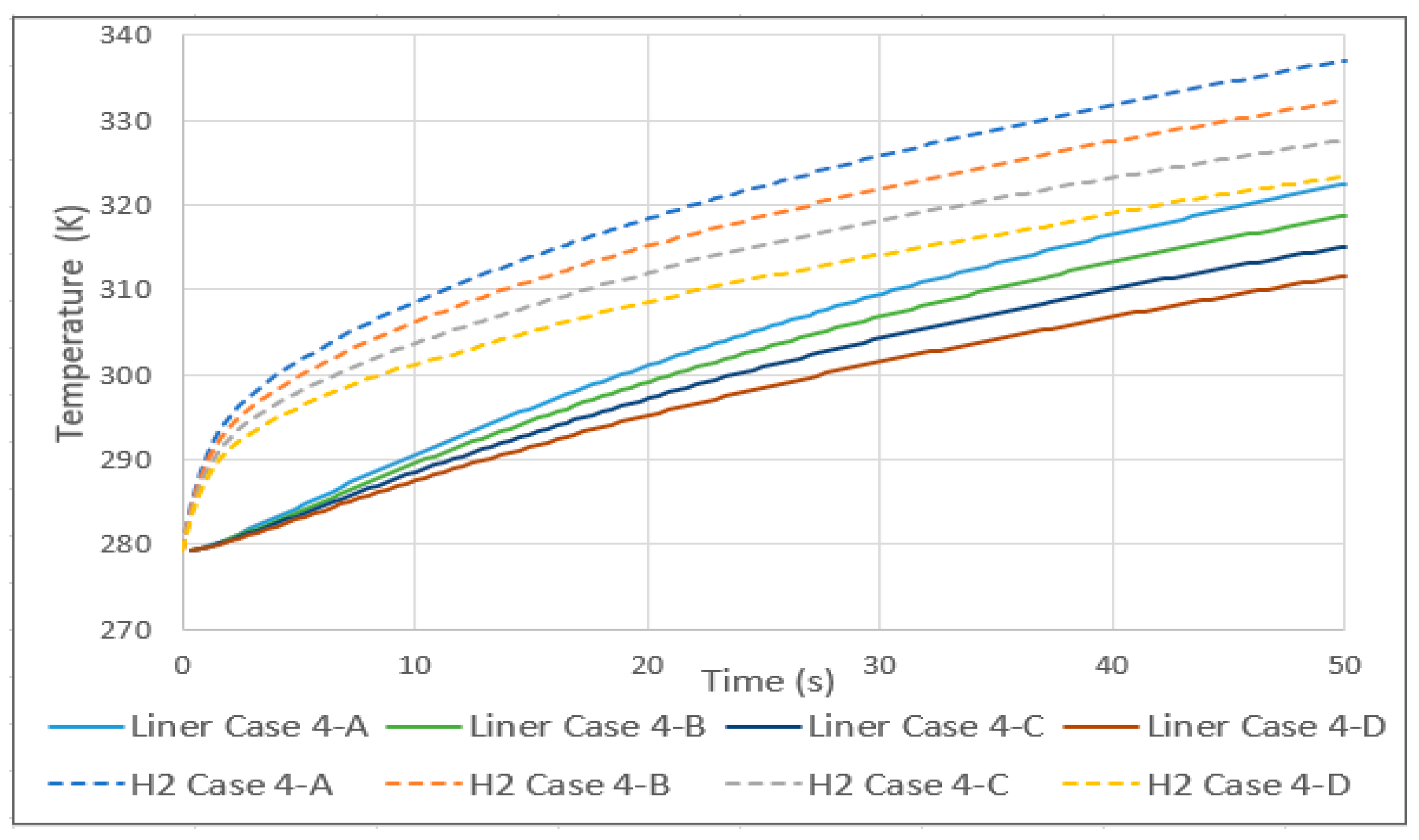
3.2. Increase in Temperature of Inlet with Fixed Equilibrium Temperature Set
3.3. Influence of Mass Flow Variation on Inlet Velocity and Temperature
3.4. Adiabatic Tank
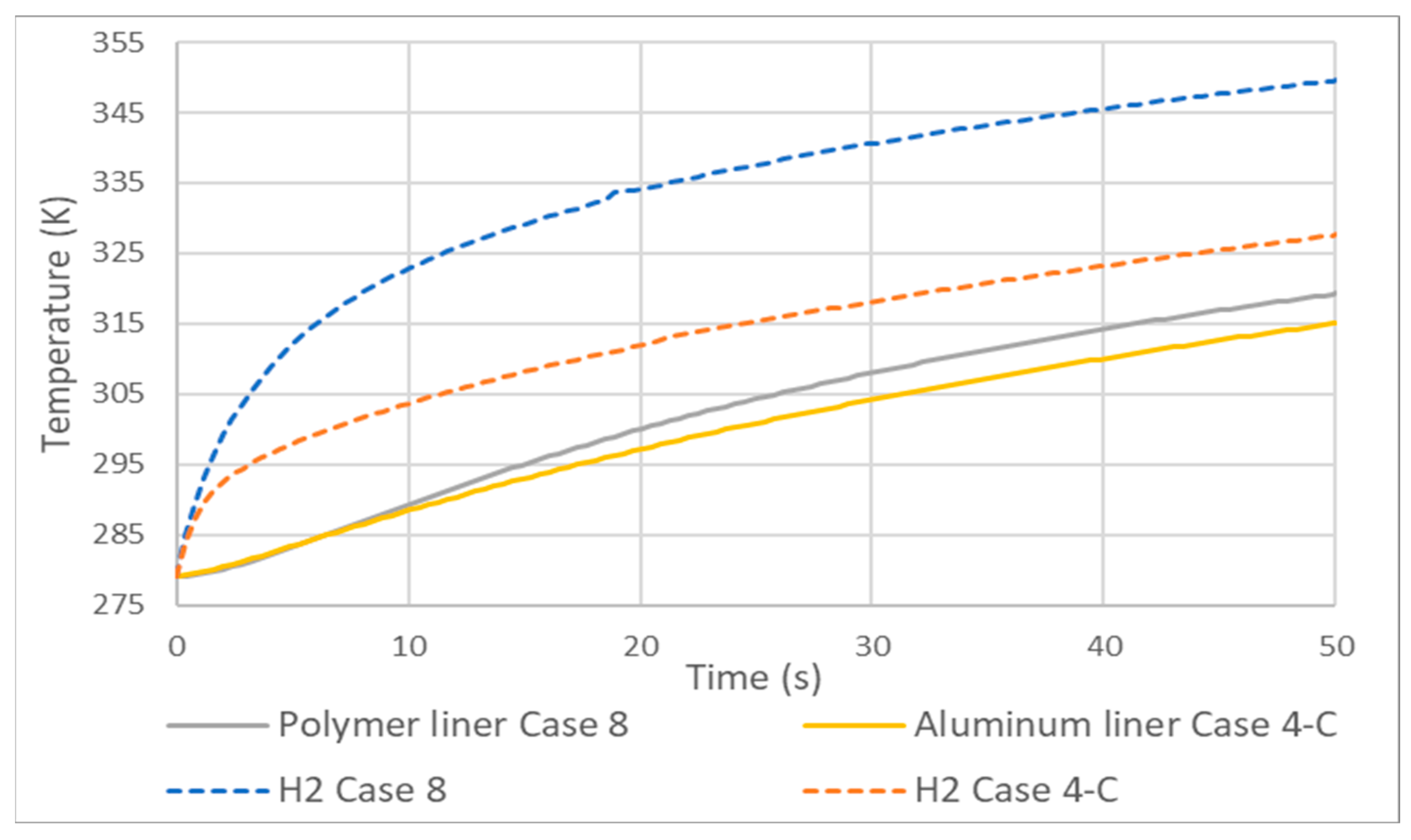
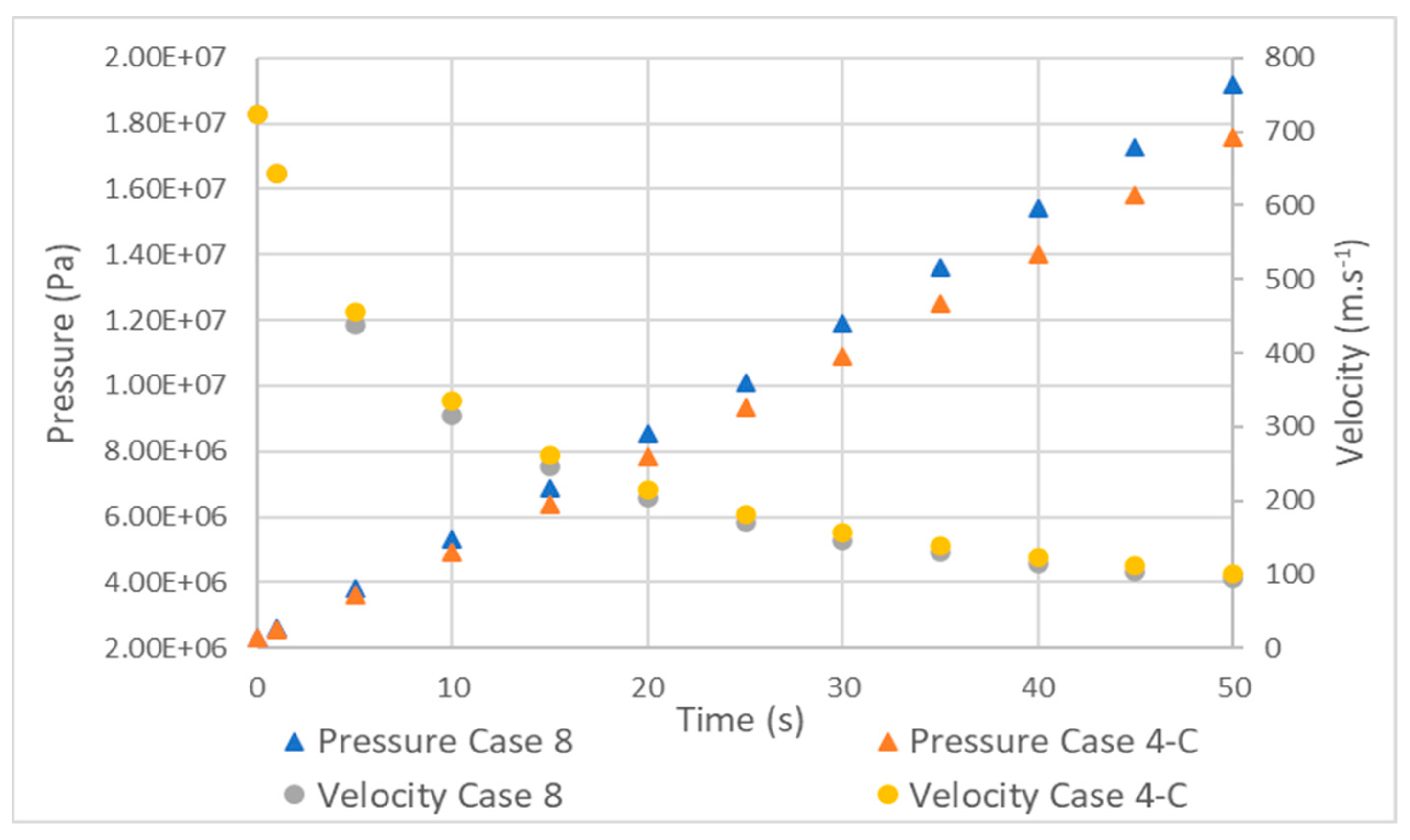
3.5. Tank Type 4
4. Conclusions
- The realizable model results were close to those of the standard, with the standard presenting slightly better results.
- A linear increase in the temperature of hydrogen occurred, both for tanks with a variable total initial thermal equilibrium and with a fixed initial tank temperature. An increase of 10 K resulted, in case 3, in an increase of 11 K in the average temperature, and in case 4, it resulted in an increase of 4.5 K.
- Due to the compressive nature of the flow, the variation in mass flow rate and, consequently, in velocity has significant implications for temperatures along the inlet tube. As the velocity increases, the difference between the static and total temperature increases and the static temperature decreases.
- Adiabatic tanks cause temperature increases in the order of 50 to 60 K relative to their non-adiabatic counterparts.
- The comparison between a type 3 and 4 tank, with the same conditions except for the lining, showed that the increase in temperature in the type 4 tank began to be significant at around 3 s and stabilized at around 30. The pressure was also greatly affected, while the velocity did not show relevant differences.
- It was also found that the Joule–Thomson effect was negligible for the current cases. The pressure difference found in the simulations was very small, resulting in a theoretical change in temperature of the centesimal order.
Author Contributions
Funding
Data Availability Statement
Conflicts of Interest
Abbreviations
| Acronyms | |
| NWP | Normal working pressure |
| SAE | Society of Automotive Engineers |
| SOC | State of charge |
| CFD | Computational fluid dynamics |
| UDF | User-defined function |
| HDPE | High-density polyethylene |
| 2D, 3D | Two-dimensional, three-dimensional |
| Cp | Specific heat at constant pressure |
| p | Pressure |
| T | Temperature |
| R | Universal gas constant of a perfect gas |
| V | Volume |
| a,b | Constants to correct for the attractive potential of molecules and volume |
| e | Turbulent dissipation rate |
| Cμ,C1 | Constants |
| REF | Reference paper for validation |
| M | Mach number |
| γ | Specific heat ratio |
| V | Local velocity |
| a | Speed of sound |
| Kronecker delta | |
| Viscosity | |
| Subscripts | |
| m | Molar |
| c | Critical |
| 0 | Total |
| i,j,k | Direction subscripts |
| eff | Effective |
| t | Turbulent |
| ‘ | Turbulent fluctuating component |
| _ | Reynolds time-averaged component |
References
- Hall, C.A.S.; Klitgaard, K.A. Energy and the Wealth of Nations, 2nd ed.; Springer: New York, NY, USA, 2012. [Google Scholar]
- Energy Information Administration. International Energy Outlook 2019; Office of Energy Analysis U.S. Department of Energy: Washington, DC, USA, 2019. [Google Scholar]
- Dawood, F.; Anda, M.; Shafiullah, G.M. Hydrogen production for energy: An overview. Int. J. Hydrogen Energy 2020, 7, 3847–3869. [Google Scholar] [CrossRef]
- Schneider, J.; Meadows, G.; Mathison, S.; Veenstra, M.; Shim, J.; Immel, R.; Wistoft-Ibsen, M.; Quong, S.; Greisel, M.; McGuire, T.; et al. Validation and Sensitivity Studies for SAE J2601, the Light Duty Vehicle Hydrogen Fueling Standard. SAE Int. J. Altern. Power. 2014, 53, 257–309. [Google Scholar] [CrossRef]
- Baptista, A.; Pinho, C.; Pinto, G.; Ribeiro, L.; Monteiro, J.; Santos, T. Assessment of an Innovative Way to Store Hydrogen in Vehicles. Energies 2019, 12, 1762. [Google Scholar] [CrossRef]
- Pinto, G.; Monteiro, J.; Baptista, A.; Ribeiro, L.; Leite, J. Study of the Permeation Flowrate of an Innovative Way to Store Hydrogen in Vehicles. Energies 2021, 14, 6299. [Google Scholar] [CrossRef]
- Ribeiro, L.; Pinto, G.F.; Baptista, A.; Monteiro, J. Study on a New Hydrogen Storage System—Performance, Permeation, and Filling/Refilling. In Hydrogen Electrical Vehicles, 1st ed.; Sankir, M., Sankir, N., Eds.; Scrivener Publishing LLC.: Beverly, MA, USA, 2023; Volume 1, pp. 11–46. [Google Scholar]
- Suryan, A.; Kim, H.D.; Setoguchi, T. Comparative study of turbulence models performance for refueling of compressed hydrogen tanks. Int. J. Hydrogen Energy 2013, 22, 9562–9569. [Google Scholar] [CrossRef]
- Cheng, Q.; Zhang, R.; Shi, Z.; Lin, J. Review of common hydrogen storage tanks and current manufacturing methods for aluminium alloy tank liners. Int. J. Lightweight Mater. Manuf. 2024, 7, 269–284. [Google Scholar] [CrossRef]
- Li, M.; Bai, Y.; Zhang, C.; Song, Y.; Jiang, S.; Grouset, D.; Zhang, M. Review on the research of hydrogen storage system fast refueling in fuel cell vehicle. Int. J. Hydrogen Energy 2019, 21, 10677–10693. [Google Scholar] [CrossRef]
- Su, Y.; Lv, H.; Zhou, W.; Zhang, C. Review of the Hydrogen Permeability of the Liner Material of Type IV On-Board Hydrogen Storage Tank. World Electr. Veh. J. 2021, 3, 130. [Google Scholar] [CrossRef]
- Hirotani, R.; Terada, T.; Tamura, Y.; Mitsuishi, H.; Watanabe, S. Thermal Behavior in Hydrogen Storage Tank for Fuel Cell Vehicle on Fast Filling; Japan Automobile Research Institute: Tokyo, Japan, 2007; 10p. [Google Scholar]
- Kim, S.C.; Lee, S.H.; Yoon, K.B. Thermal characteristics during hydrogen fueling process of type IV cylinder. Int. J. Hydrogen Energy 2010, 13, 6830–6835. [Google Scholar] [CrossRef]
- Zhao, Y.; Liu, G.; Liu, Y.; Zheng, J.; Chen, Y.; Zhao, L.; Guo, J.; He, Y. Numerical study on fast filling of 70 MPa type III cylinder for hydrogen vehicle. Int. J. Hydrogen Energy 2012, 22, 17517–17522. [Google Scholar] [CrossRef]
- Liu, Y.-L.; Zhao, Y.-Z.; Zhao, L.; Li, X.; Chen, H.-G.; Zhang, L.-F.; Zhao, H.; Sheng, R.-H.; Xie, T.; Hu, D.-H.; et al. Experimental studies on temperature rise within a hydrogen cylinder during refueling. Int. J. Hydrogen Energy 2010, 7, 2627–2632. [Google Scholar] [CrossRef]
- Zheng, J.; Guo, j.; Yang, J.; Zhao, Y.; Zhao, L.; Pan, X.; Ma, J.; Zhang, L. Experimental and numerical study on temperature rise within a 70 MPa type III cylinder during fast refueling. Int. J. Hydrogen Energy 2013, 25, 10956–10962. [Google Scholar] [CrossRef]
- Galassi, M.C.; Baraldi, D.; Iborra, B.A.; Moretto, P. CFD analysis of fast filling scenarios for 70 MPa hydrogen type IV tanks. Int. J. Hydrogen Energy 2012, 8, 6886–6892. [Google Scholar] [CrossRef]
- Miguel, N.; Acosta, B.; Moretto, P.; Cebolla, R.O. Influence of the gas injector configuration on the temperature evolution during refueling of on-board hydrogen tanks. Int. J. Hydrogen Energy 2016, 42, 19447–19454. [Google Scholar] [CrossRef]
- Kesana, N.R.; Welahettige, P.; Hansen, P.M.; Ulleberg, Ø.; Vågsæther, K. Modelling of fast fueling of pressurized hydrogen tanks for maritime applications. Int. J. Hydrogen Energy 2023, 79, 30804–30817. [Google Scholar] [CrossRef]
- Melideo, D.; Baraldi, D.; Galassi, M.C.; Cebolla, R.O.; Iborra, B.A.; Moretto, P. CFD model performance benchmark of fast filling simulations of hydrogen tanks with pre-cooling. Int. J. Hydrogen Energy 2014, 9, 4389–4395. [Google Scholar] [CrossRef]
- Wang, G.; Zhou, J.; Hu, S.; Dong, S.; Wei, P. Investigations of filling mass with the dependence of heat transfer during fast filling of hydrogen cylinders. Int. J. Hydrogen Energy 2014, 9, 4380–4388. [Google Scholar] [CrossRef]
- Ortiz Cebolla, R.; Acosta, B.; de Miguel, N.; Moretto, P. Effect of precooled inlet gas temperature and mass flow rate on final state of charge during hydrogen vehicle refueling. Int. J. Hydrogen Energy 2015, 40, 4698–4706. [Google Scholar] [CrossRef]
- Melideo, D.; Baraldi, D.; Iborra, B.A.; Cebolla, R.O.; Moretto, P. CFD simulations of filling and emptying of hydrogen tanks. Int. J. Hydrogen Energy 2017, 11, 7304–7313. [Google Scholar] [CrossRef]
- Ansys. ANSYS Fluent User Guide; Ansys Fluent; Ansys: Canonsburg, PA, USA, 2022. [Google Scholar]
- AIAA. Guide for the Verification and Validation of Computational Fluid Dynamics Simulations (AIAA G-077-1998(2002)); American Institute of Aeronautics and Astronautics, Inc.: Washington, DC, USA, 1998. [Google Scholar]
- Miguel, N.; Cebolla, R.O.; Acosta, B.; Moretto, P.; Harskamp, F.; Bonato, C. Compressed hydrogen tanks for on-board application: Thermal behaviour during cycling. Int. J. Hydrogen Energy 2015, 19, 6449–6458. [Google Scholar] [CrossRef]
- Suryan, A.; Kim, H.D.; Setoguchi, T. Three dimensional numerical computations on the fast filling of a hydrogen tank under different conditions. Int. J. Hydrogen Energy 2012, 9, 7600–7611. [Google Scholar] [CrossRef]
- Nasrifar, K. Comparative study of eleven equations of state in predicting the thermodynamic properties of hydrogen. Int. J. Hydrogen Energy 2010, 8, 3802–3811. [Google Scholar] [CrossRef]
- Kim, M.-S.; Ryu, J.-H.; Oh, S.-J.; Yang, J.-H.; Choi, S.-W. Numerical Investigation on Influence of Gas and Turbulence Model for Type III Hydrogen Tank under Discharge Condition. Energies 2020, 23, 6432. [Google Scholar] [CrossRef]
- Magi, V.I.J.A.V. The k-ε Model and computed spreading rates in round and plate jets. Numer. Heat Transf. A Appl. 2001, 4, 317–334. [Google Scholar]
- Kim, M.-S.; Jeon, H.-K.; Lee, K.-W.; Ryu, J.-H.; Choi, S.-W. Analysis of Hydrogen Filling of 175 Liter Tank for Large-Sized Hydrogen Vehicle. Appl. Sci. 2022, 12, 4856. [Google Scholar] [CrossRef]
- Galassi, M.C.; Papanikolaou, E.; Heitsch, M.; Baraldi, D.; Iborra, B.A.; Moretto, P. Assessment of CFD models for hydrogen fast filling simulations. Int. J. Hydrogen Energy 2014, 11, 6252–6260. [Google Scholar] [CrossRef]
- Miguel, N.; Acosta, B.; Baraldi, D.; Melideo, R.; Cebolla, R.O.; Moretto, P. The role of initial tank temperature on refuelling of on-board hydrogen tanks. Int. J. Hydrogen Energy 2016, 20, 8606–8615. [Google Scholar] [CrossRef]
- Acosta, B.; Moretto, P.; Miguel, N.; Ortiz, R.; Harskamp, F.; Bonato, C. JRC reference data from experiments of on-board hydrogen tanks fast filling. Int. J. Hydrogen Energy 2014, 35, 20531–20537. [Google Scholar] [CrossRef]
- Glenn Research Center. Speed of Sound; NASA: Washington, DC, USA, 2021. Available online: https://www.grc.nasa.gov/www/BGH/snddrv.html (accessed on 14 June 2023).
- Ansys. ANSYS Fluent Theory Guide; Ansys Fluent; Ansys: Canonsburg, PA, USA, 2022. [Google Scholar]


| Type | Materials | Pressure Range | Features |
|---|---|---|---|
| Type 1 | All metal (steel and aluminum) | 17.5–20 | Heavy, internal corrosion. |
| Type 2 | Metal liner with hoop wrapping | 26.3–30 | Heavy, internal corrosion. |
| Type 3 | Metal liner (aluminum) with full composite wrapping (carbon fiber) | 35–70 | Lightness, low permeation, galvanic corrosion between liner and fiber, high burst pressure. |
| Type 4 | Polymer (thermoplatic) liner with full composite wrapping (carbon fiber) | 35–70 | Lightness, high permeation, relatively low burst pressure, no creep fatigue, simple manufacturability. |
| Internal Length (m) | Inner Radius (m) | Liner Thickness (m) | Laminate Thickness (m) |
|---|---|---|---|
| 0.702 | 0.145 | 0.004 | 0.015 |
| Simulations | Inlet Temperature (K) | Initial Temperature (K) | Mass Flow Rate (kg·s−1) | Exterior Temperature (K) |
|---|---|---|---|---|
| Case 1 | UDF | 293 | 0.008 | 293 |
| Case 2 | UDF | 293 | 0.008 | 293 |
| Case 3-A | 313 | 313 | 0.008 | 313 |
| Case 3-B | 303 | 303 | 0.008 | 303 |
| Case 3-C | 293 | 293 | 0.008 | 293 |
| Case 3-D | 283 | 283 | 0.008 | 283 |
| Case 4-A | 313 | 279 | 0.008 | 313 |
| Case 4-B | 303 | 279 | 0.008 | 303 |
| Case 4-C | 293 | 279 | 0.008 | 293 |
| Case 4-D | 283 | 279 | 0.008 | 283 |
| Case 5-A | 303 | 303 | 0.008 | adiabatic |
| Case 5-B | 293 | 293 | 0.008 | adiabatic |
| Case 5-C | 283 | 283 | 0.008 | adiabatic |
| Case 6-A | 293 | 279 | 0.01 | 293 |
| Case 6-B | 293 | 279 | 0.006 | 293 |
| Case 6-C | 293 | 279 | 0.004 | 293 |
| Case 6-D | 293 | 279 | 0.002 | 293 |
| Case 7-A | 293 | 279 | 0.008 | adiabatic |
| Case 7-B | 293 | 279 | 0.006 | adiabatic |
| Case 7-C | 293 | 279 | 0.004 | adiabatic |
| Case 8 | 293 | 279 | 0.008 | 293 |
| Parameter | Value |
|---|---|
| Solver | Pressure-based (segregated) [19,31] |
| Pressure–Velocity coupling | SIMPLE [14,16] |
| Spatial discretization | Second-order/second-order UPWIND [31] |
| Temporal discretization | Second-order implicit [32] |
| Gradient discretization | Least-squares cell-based |
| Hydrogen Final Temperature (K) | Aluminum Liner Final Temperature (K) | |
|---|---|---|
| Realizable case 2 | 320.177 | 313.118 |
| Standard case 1 | 319.104 | 312.633 |
| Final Pressure (MPa) | Initial Velocity (m·s−1) | Final Velocity (m·s−1) | |
|---|---|---|---|
| Case 3-A | 19 | 769 | 100.5 |
| Case 3-B | 18.5 | 746 | 100 |
| Case 3-C | 18 | 723 | 99.5 |
| Case 3-D | 17.5 | 700 | 99 |
| 5-A and 3-B (303 K) | 5-B and 3-C (293 K) | 5-C and 3-D (283 K) | |
|---|---|---|---|
| Temperatures (K) | +56 | +54 | +52 |
| 7-A and 4-C (8 g/s) | 7-B and 6-B (6 g/s) | 7-C and 6-C (4 g/s) | |
|---|---|---|---|
| Temperatures (K) | +60 | +61 | +60 |
Disclaimer/Publisher’s Note: The statements, opinions and data contained in all publications are solely those of the individual author(s) and contributor(s) and not of MDPI and/or the editor(s). MDPI and/or the editor(s) disclaim responsibility for any injury to people or property resulting from any ideas, methods, instructions or products referred to in the content. |
© 2024 by the authors. Licensee MDPI, Basel, Switzerland. This article is an open access article distributed under the terms and conditions of the Creative Commons Attribution (CC BY) license (https://creativecommons.org/licenses/by/4.0/).
Share and Cite
Monteiro, J.M.; Ribeiro, L.; Monteiro, J.; Baptista, A.; Pinto, G.F. Computational Fluid Dynamics Simulation of Filling a Hydrogen Type 3 Tank at a Constant Mass Flow Rate. Energies 2024, 17, 1375. https://doi.org/10.3390/en17061375
Monteiro JM, Ribeiro L, Monteiro J, Baptista A, Pinto GF. Computational Fluid Dynamics Simulation of Filling a Hydrogen Type 3 Tank at a Constant Mass Flow Rate. Energies. 2024; 17(6):1375. https://doi.org/10.3390/en17061375
Chicago/Turabian StyleMonteiro, José Miguel, Leonardo Ribeiro, Joaquim Monteiro, Andresa Baptista, and Gustavo F. Pinto. 2024. "Computational Fluid Dynamics Simulation of Filling a Hydrogen Type 3 Tank at a Constant Mass Flow Rate" Energies 17, no. 6: 1375. https://doi.org/10.3390/en17061375
APA StyleMonteiro, J. M., Ribeiro, L., Monteiro, J., Baptista, A., & Pinto, G. F. (2024). Computational Fluid Dynamics Simulation of Filling a Hydrogen Type 3 Tank at a Constant Mass Flow Rate. Energies, 17(6), 1375. https://doi.org/10.3390/en17061375