Article

Low-Cost System with Transient Reduction for Automatic Power Factor Controller in Three-Phase Low-Voltage Installations

by
Gabriel Nicolae Popa
* and
Corina Maria Diniș
Department of Electrical Engineering and Industrial Informatics, Politehnica University of Timișoara, 5 Revolution Street, 331128 Hunedoara, Romania
*
Author to whom correspondence should be addressed.
Energies 2024, 17(6), 1363; https://doi.org/10.3390/en17061363
Submission received: 3 February 2024 / Revised: 1 March 2024 / Accepted: 8 March 2024 / Published: 12 March 2024
(This article belongs to the Special Issue Microcontrollers Systems and PLCs Used in Energies)

Abstract

:
In power engineering, the importance of maintaining a high power factor in low-voltage electrical installations is known. In power substations for industry, the usual method of coupling is to use an automatic power factor controller which connects capacitors banks (with electromagnetic contactors). Sometimes, AC reactors are connected to the phases of the capacitors banks (to reduce transient phenomena and the deforming regime), depending on the desired value of the power factor. This paper presents an analysis (more focused on experimentation) of a low-cost system for automatic regulation of the power factor with a reduction in transients and an increase in the life of contactors (eliminating the electric arc during switching on), with capacitors banks for low-voltage three-phase installations that connect the capacitors banks by means of one three-phase solid-state relay (an expensive device for a quality device; one is used for all capacitors banks) and using several electromagnetic contactors. The automatic power factor adjustment system has a controller with a microprocessor with six outputs, controlled by the phase shift between the current (measured with a current transformer proportional to the current in a bar) and the phase voltage, which is part of a system of distribution bars (L1,2,3, N) from which electrical consumers (e.g., induction motors) are supplied. To reduce transients when connecting capacitors banks, a three-phase solid-state relay and two related electromagnetic contactors are used for each capacitors bank. The automatic power factor controller is connected to two low-capacity PLCs that control the logic of connecting the capacitors banks to reduce transients. By using the proposed regulation system, a cheaper control solution is obtained compared to the use of one solid-state relay for each capacitors banks, under the conditions in which the power factor adjustment is made as in the classic solution. If twelve capacitors banks are used, the proposed installation is 22.57% cheaper than the classical power factor regulation installation.

Graphical Abstract

1. Introduction

There have been concerns for a long time, even before the development of electronics, to introduce automatic power factor controllers in low-voltage electrical installations. Along with the development of electronics, electronic power factor controllers were made with discrete components, which were used to measure current, voltage and the phase shift between them, and then a DC voltage proportional to the reactive power in the network was determined. This DC voltage is compared to two voltage references to create hysteresis proportional to the power factor (PF) desired in the installation. The electronic circuit determines the timed switching on and switching off of capacitors banks (CBs) from or into the installation. In the case of electrical consumers connected for a long period to the network, to improve the PF, CBs may be permanently connected to inductive electrical consumers (resonances may occur when connecting the voltage), or an automatic power factor controller (APFC; also known as a Reactive Power Controller) with discrete electronic components that allows the control of the PF in the installation according to the measured current or according to a programmed clock may be used [1,2,3].
With the invention of microprocessors and digital signal processors, there were concerns in making high-performance APFCs for single-phase (less often) or three-phase installations. In the vast majority of PFCs, the phase shift between voltage and current is measured, and then the determined value is compared to the set values of the PF. They can be connected by electromagnetic contactors (EMCs) or they can be connected by high-frequency controlled power drivers (the commutation frequency changes with the reactance of the load), controlled by the microprocessor [4].
When a capacitance load is switched on to the power supply, it begins to draw a very large inrush current (which depends on the moment of time when the connection is made and the initial voltage load on the capacitor), which drops quickly. The inrush current is large enough to significantly exceed the maximum allowed exchange current for the contactor contacts. When capacity is fully discharged, this inrush current is limited only by the parasitic resistance between contact and load capacity. As the load increases, the current decreases. For contactors, the switching-on moment is the biggest problem: contacts carry the maximum current (electrical contacts will wear out prematurely), and even when this current exceeds the maximum permitted, it can be continued for a short time. The inrush current in a capacitor circuit is tens of times higher than the steady-state current. When disconnecting the capacitors from the network, no current shocks are recorded [5,6,7].
The development of power electronics has led to the development of solid-state relays (SSRs) with semiconductors, which can successfully replace, in the vast majority of applications, the classical EMCs with contacts. Also, SSRs (more complicated in terms of control than those that control resistive and inductive loads) were built for capacitive loads. Due to the advantages they have, nowadays zero-voltage switching SSRs (Z type) are used together with APFCs to regulate the PF in electrical installations. Electronic solid-state relays are increasingly used in electrical control installations for switching on and switching off electrical power consumers. For high power, SSRs are mounted on radiators. The command is made with DC voltage and is optically isolated from the power output (it usually consists of two thyristors connected in anti-parallel), so that galvanic separation can be ensured [8,9].
The PF improvement plant with a classical APFC is known which permanently measures the line current, usually with a current transformer (CT), and the voltage on the same phase (or in other types of regulators, the line voltage on the other two phases), and depending on the calculated and imposed value of the PF, the CBs are timed to switching-switch on or switch off one by one, through the related contactors. The total reactive power of the CBs is set according to the reactive power to be compensated, and the number of banks, according to the fineness of the PF adjustment. The disadvantages of this installation are the current peaks generated by the CBs that occur when they are connected and the premature wear of the contactor contacts.
These disadvantages are removed by a similar installation in which the EMCs are replaced with three-phase power SSRs and the switching on of the CBs is performed when the voltage crosses zero, in turn, on each phase in part. The lifetime of three-phase power SSRs is much longer than that of EMCs, and their control can be accomplished with low DC voltages (3–32 V DC). The disadvantage of this installation is that it costs 3–5 times greater, depending on the number of steps of CBs, compared to the previous version [10,11,12].
APFCs for single-phase electrical installations are known. In such a PFC, the installation contains a voltage transformer whose secondary connects with a capacitor, and the primary of the transformer connects to the output of an autotransformer. To measure the phase shift between voltage and current, transducers are used, which control the rotor (cursor) of the autotransformer by means of an electric servo drive. By changing the output voltage of the autotransformer, the reactive power of the capacitor can be changed, and implicitly, also, of the PF in the network [2,5].
It is known about APFC designs with microcontrollers, microprocessors and digital signal processors. In some PFCs, PF measurements can be made at medium or low voltage. APFCs that measure low voltage current factors can use SCADA monitoring and control for power substation groups. The APFC can determine at which point in the installation a CB can be switched on/switched off. Some APFCs include a stabilization component of the supply voltage in addition to the measurement component. Current measurements in the installation can be performed with CTs (the classic type) or, more easily, with amp clamps [13,14,15,16].
Some APFCs are built using programmable logic controllers (PLCs), and PFs are measured by a CT in power substations for medium and low-voltage installations. When switching on the CBs to reach the pre-defined PF, the unbalance between voltage and current is taken into account. Other PFCs are designed based on active and apparent power measurement and are known to determine PFs and compare PFs with the binding values [17,18,19,20].
Normally, the vast majority of APFCs in three-phase electrical installations measure the line current (the most loaded) and the corresponding phase voltage, or in other systems the other two phase voltages. These types of PFCs have the disadvantage of introducing the same capacitor into three phases, regardless of the load per phase and the type of load per phase. The PFC is known to have a microcontroller that measures the current and voltage in three phases (the signals are measured and galvanically separated), and through a power driver it introduces a capacitor with different values in each phase. This APFC is suited to highly unbalanced electrical consumers [21,22,23,24,25,26].
SSRs can be commonly used to control resistive and inductive electrical loads. When controlling capacitive loads, special SSRs must be used, which have a complex control system, which requires a detailed theoretical, simulated and experimental study (which is not the subject of this paper). In some researches, analyzes were made, especially experimental ones, regarding the operation of SSRs [27,28]. The current work focuses on the practical verification of the PF regulation concept with classic PFCs for switching on/switching off CBs with a single three-phase SSR.
The paper is divided into five sections. The Section 2 is about materials and methods and presents a theoretical and simulation analysis of ideal and real capacitors that are switched on at sinusoidal and non-sinusoidal voltages, the electrical diagram of classical APFC, the low-cost APFC with the reduction in transients and increasing the life of contactors, with capacitors banks, one three-phase SSR, PLCs and using several EMCs. In the same section, the program implemented in the PLC is presented, with different operating phases during the monitoring period, and then a comparative economic analysis is made between two types of APFC installations. The Section 3 presents the experimental results (three groups of experiments are presented) with capacitors, CBs, an SSR and an APFC (with CBs and CBs connecting with an AC reactor). The Section 4 is a discussion of the use of a low-cost system with a reduction in transients for automatic adjustment of the power factor. Conclusions on the use of the proposed low-cost APFC are presented in the last section (Section 5).

2. Materials and Methods

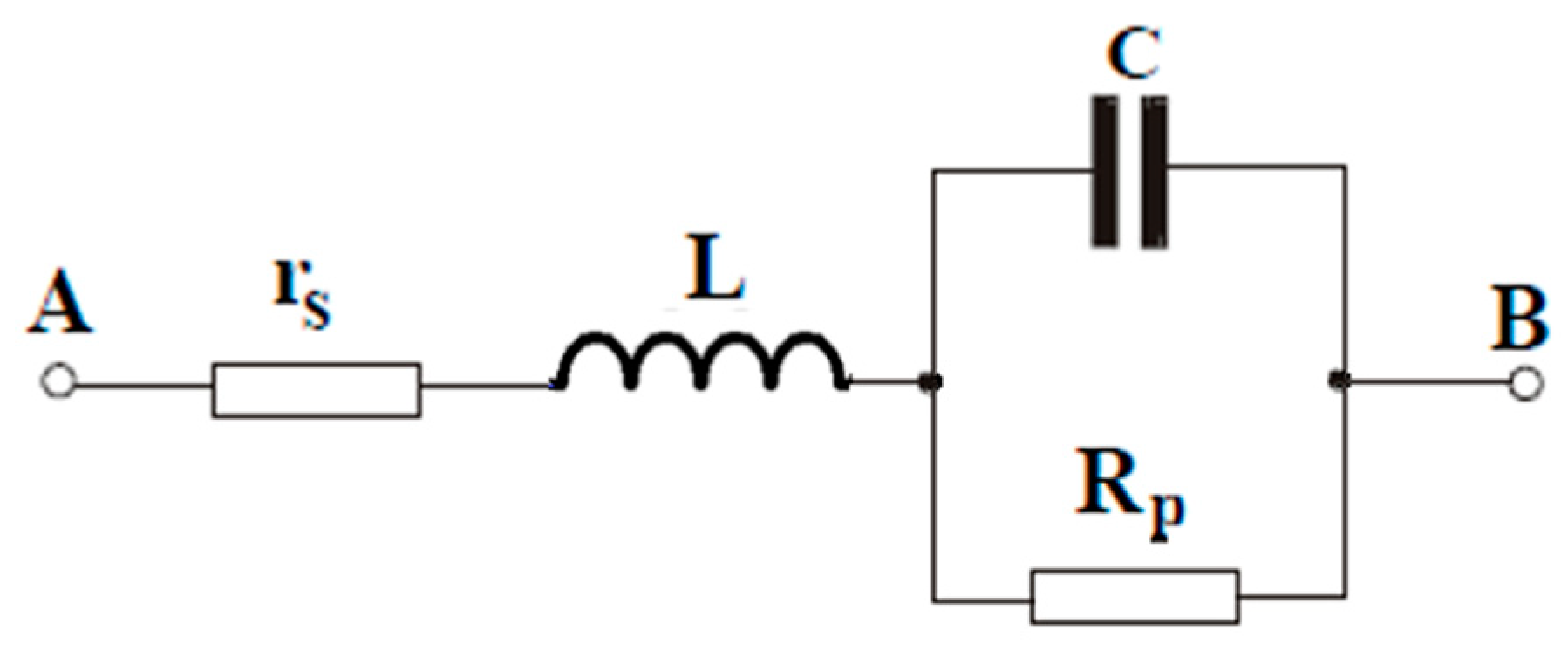
2.1. Analysis of Currents through Real Capacitors

If it consider an ideal sinusoidal voltage, which has the RMS value U1 and the pulsation ω, the instantaneous voltage can be expressed as:
u t = 2 · U 1 · sin ( ω · t )
to which an ideal capacitor (lossless) C is connected, which has capacitive reactance:
X C = 1 ω · C
then the current passing through the capacitor is determined by:
i t = 2 · I 1 · sin ω · t + π 2 = 2 · U 1 · ω · C · sin ( ω · t + π 2 )
where I1 is the RMS current.
So, the current is sinusoidal (just like the voltage) and out of phase by 90° before the voltage (Figure 1).
The RMS value of the current is calculated with:
I 1 = U 1 X C = U 1 · ω · C
In reality, the supply voltage is not sinusoidal [1,2], and the instantaneous voltage can be expressed as:
u t = U 0 + k = 1 n u k t = U 0 + k = 1 n 2 · U k · sin ( k · ω · t + α k )
where U0 is the continuous component of the voltage, k (integer) is the rank of the harmonics, Uk the RMS value of the voltage of rank k, and αk is the initial phase shift of the harmonic of rank k; n is an integer (theoretically it has an infinite value) and, usually, in practice it takes the value 50 (there is a limit to the harmonics taken into account so that the measuring equipment can calculate in real time) [3].
The RMS value of the voltage is calculated with:
U = U 0 2 + k = 1 n U k 2
In general, the impedance is not constant with frequency, and the impedance at a harmonic k is:
Z k = U k I k
The instantaneous of the current passing through a circuit supplied with a non-sinusoidal voltage is:
i t = I 0 + k = 1 n i k t = I 0 + k = 1 n 2 · I k · sin ( k · ω · t + α k + β k )
where I0 is the continuous component of the current, Ik the RMS value of the current of order k, and βk is the phase shift between the harmonics of order k of current and voltage.
The current can also be written in terms of harmonic voltages and harmonic impedances:
i t = I 0 + k = 1 n 2 · U k Z k · sin ( k · ω · t + α k + β k )
The RMS value of the current is calculated with:
I = I 0 2 + k = 1 n I k 2
If we consider an ideal capacitor of value C, whose reactance XCk changes with frequency, supplied at a non-sinusoidal voltage (5) where U0 is neglected, the current can be written:
i t = k = 1 n 2 · U k X C k · sin ( k · ω · t + α k + φ k ) = k = 1 n 2 · U k · k · ω · C · sin ( k · ω · t + α k + φ k )
where XCk is the capacitive reactance at frequency k, determined by:
X C k = 1 k · ω · C
From Equation (11) it can be seen that, even if the voltage is slightly non-sinusoidal, with the increase in frequency, the current becomes more non-sinusoidal compared to the voltage applied to the capacitor (basically, the capacitor due to its operating principle amplifies current harmonics).
A real capacitor has the electrical model shown in Figure 2 [11].
In Figure 2, rs is the equivalent series resistance of the capacitor, L is the inductance determined by the design of the capacitor, C is the ideal capacity, and Rp is the loss resistance. The real capacitor in Figure 2 has the impedance, at the fundamental frequency:
Z _ A B = r s + j · ω · L j · R p ω · C R p j · 1 ω · C
and for harmonics of order k it is:
Z _ A B k = r s + j · k · ω · L j · R p k · ω · C R p j · 1 k · ω · C
The current passing through the real capacitor is determined by:
i t = k = 1 n 2 · U k Z A B k · sin ( k · ω · t + α k + γ k )
and the RMS value of the current is:
I = k = 1 n U k 2 Z A B k 2
The total harmonic distortion factor for voltage is calculated with:
T H D U = k = 2 50 U k 2 U 1 · 100
and the total harmonic distortion factor for current is calculated with:
T H D I = k = 2 50 I k 2 I 1 · 100
To determine the parameters of the real capacitor, they must be measured at various frequencies corresponding to the k current harmonics (difficult to achieve practically).
The measurements for the supply voltage (real) in Figure 3 and Table 1 were made with a CA 8334B power quality analyzer (Chauvin Arnoux, Lille, France), in order to show the non-sinusoidal waveform (THDU = 3.1%).
In Figure 4, Figure 5, Figure 6 and Figure 7, simulations were made with a real capacitor (Figure 2). The approximate parameters of the 15 µF capacitor are (Figure 2): rs = 0.34 Ω; L = 0.1 mH; C = 15 µF; Rp = 50 MΩ.
From Figure 4 and Figure 5, it can be seen that the initial phase of the voltage determines the value for the inrush current of the capacitor. If the initial phase is 0° (Figure 4) then the inrush current is much lower (over 20 times) compared to connecting the capacitor at maximum voltage (90°, Figure 5). Initially, the inrush current has an oscillating transient regime that lasts a short time (2 ms), after which the signal stabilizes for approx. two periods. In steady-state mode, it is observed that the inrush current is sinusoidal and out of phase before the voltage.
When applying the non-sinusoidal voltage as in Figure 7, in steady-state mode, the same shape of the signals as in Figure 6b is obtained.
If a non-sinusoidal voltage is applied (like the real one in Figure 3, Table 1), then the transient regime for inrush current lasts a little longer (3 ms) compared to the previous cases, and when applying the maximum voltage on the capacitor (Figure 7) a current more than 20 times higher is obtained compared to the case when zero voltage is applied to the capacitor (Figure 6). In order to reduce the value of inrush current, switching must be carried out when the voltage crosses zero. What is important is the fact that in steady-state mode the current is much more distorted compared to the voltage (confirmed by practice), and the current is ahead of the voltage—Figure 6b. So, for a capacitor, a small deformation of the voltage waveform causes a deep deformation of the current.

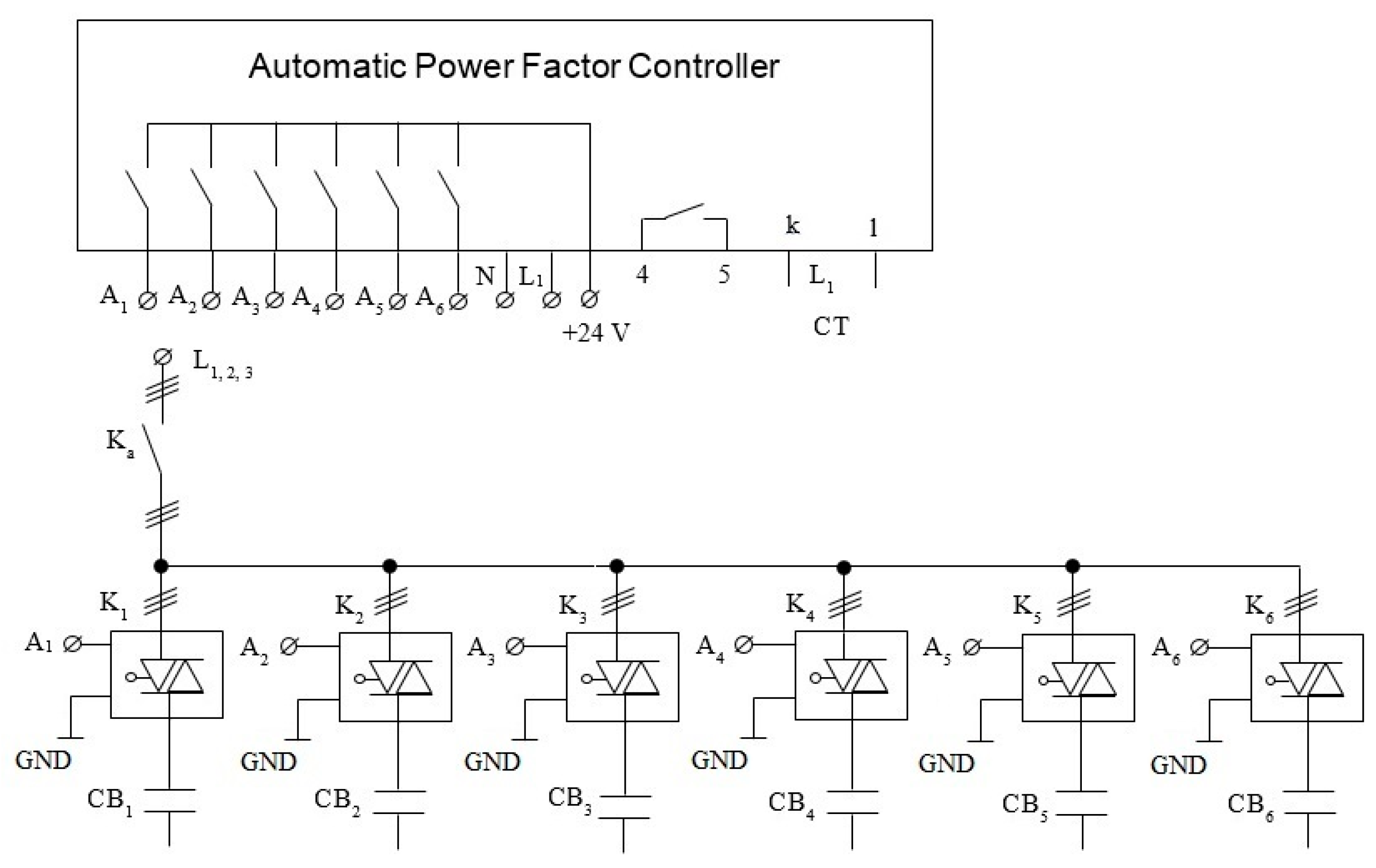
2.2. Automatic Power Factor Controller

We further present an installation for PF improvement in three-phase low-voltage installations using an APFC (classical), low-capacity PLCs, EMCs, a three-phase power SSR and CBs for PF improvement.
The PF improvement installation with a classical APFC is known (Figure 8). The current (line, the most loaded) is permanently measured, usually with a CT, and the voltage on the same phase (or with other types of regulators, the line voltage on the other two phases), and depending on the calculated and set value of the PF, the CBs (CB1, CB2, CB3, CB4, CB5, CB6) are timed to switch on or switch off through the related EMCs (K1, K2, K3, K4, K5, K6). The capacitor banks are set according to the reactive power, and the number of CBs according to the fineness of the power factor adjustment. In modern APFCs, the presence of harmonics in the network is constantly monitored, as well as the temperature level of the enclosure where the CBs are located. The disadvantages of the classical installation are the current peaks that pass through the CBs when they are connected (the switching is performed at random voltages, between −Vmax and Vmax) and the premature wear of the EMCs’ contacts (reducing their life span).
To eliminate the disadvantages of the installation in Figure 8, an installation with a similar function can be made, as in Figure 9, where the EMCs are replaced with three-phase power solid-state relays (SSRs), and the switching is performed when the voltage crosses zero, in turn, on each phase. The lifetime of SSRs (expensive devices) is much longer, and their control can be accomplished with low DC voltages (3–32 V, DC). The disadvantage of this installation that is the costs are 3–5 times greater, depending on the number of steps, compared to the installation in Figure 8.
The solid-state relay is an electronic device with no moving parts, since the mechanical electrical contacts have been replaced by thyristors or triacs (for AC applications). The electrical separation between the input control signal and the output load voltage is achieved using an opto-coupler type light sensor. A solid-state relay is equivalent to the use of an electromechanical relay and can be used to control electrical loads without the use of classic electrical contacts [8,9].
A solid-state relay ensures a high degree of reliability, long life and reduced electromagnetic interference during the switching process, and the response time is much faster, almost instantaneous, compared to a conventional electromechanical relay. Also, the power requirements for driving the input of a solid-state relay are generally low enough to make them compatible with most logic families. However, being a power semiconductor device, they must be mounted on a suitable heatsink to prevent heating of the semiconductor device during steady state operation (the voltage drop on the SSR is approx. 1.7 V, AC).
Solid-state relays have the following advantages over classic relays [29,30]:
  • they have no moving parts;
  • they can operate at high switching-on/switching-off frequencies;
  • switching times are lower;
  • the control can be applied when the voltage passes through zero, so that when starting the consumer absorbs a small current;
  • they are more reliable than classic electromagnetic contactors.

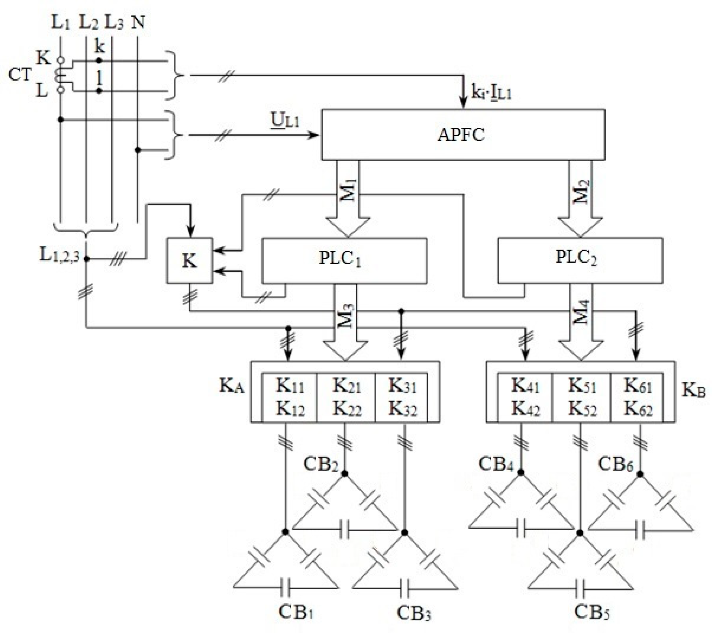
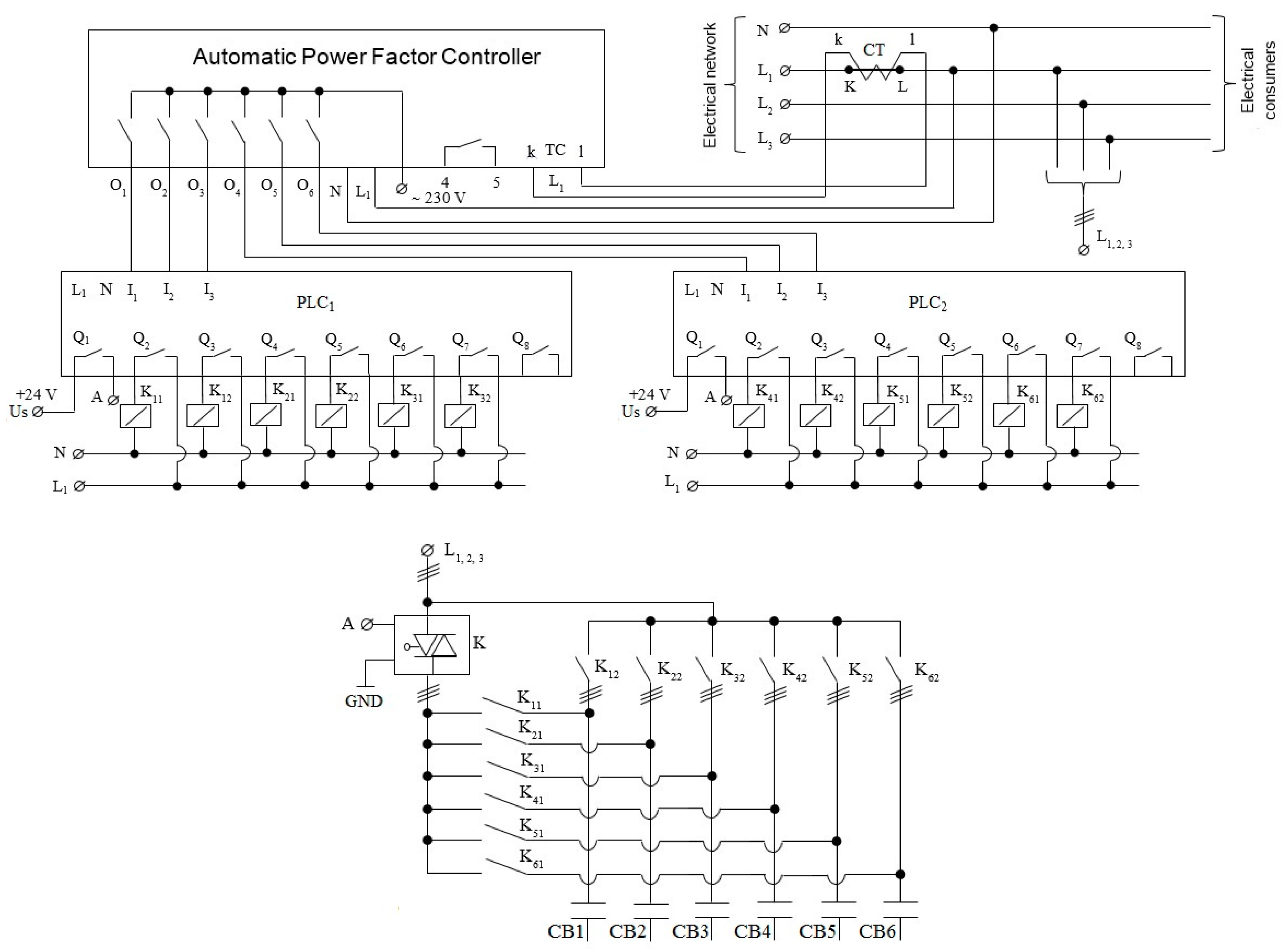
2.3. Low-Cost Automatic Power Factor Controller

This paper refers to a low-cost system for automatic adjustment of the power factor with capacitors banks in three-phase low-voltage installations that reduces transients (at the switching on of capacitors banks) and eliminates the electric arc when connecting the capacitors banks.
Figure 10 shows the graphs, as a function of time, of the voltage and current when a capacitor is switched on through a classical EMC (on the left side of the image), and through the SSR, where the switching takes place when the voltage crosses zero power supply (on the right side of the image). In the first case, the current when connecting the capacitor can increase to more than eight times than the nominal value, which causes a decrease in the reliability of classical EMCs (reduces the lifetime of the contacts) and, implicitly, of the APFC.
Compared to the classical APFC, the proposed PF installation (Figure 11) uses the control signals from the classical APFC with a microprocessor, which measures the voltage and current in the power substation; the signals are then sent to the PLC (if the PLC has too few inputs and outputs, several PLCs or extension modules can be used), which through a specific program, in turn, controls a group of EMCs and one three-phase power SSR to switch on the CBs to the electrical installation. The program in the PLC is implemented in such a way that the connection of the CBs is made through a three-phase SSR (switching is performed when the voltage crosses zero), and the permanent power supply of the CBs is provided through EMCs. The proposed PF improvement APFC lends itself to controlling a large number of CBS (from three to twelve CBs, depending, also, on the inputs and outputs of the PLCs), so that the expenses will be considerably lower than in the classical installation.
The proposed technical solution consists in creating a low-cost system for automatic control of the PF and the reduction in transients, with CBs from low-voltage three-phase installations, which use a single three-phase power SSR, common to all steps of the CBs (one SSR is no longer used for each CB, as in Figure 9).
The low-cost system for automatic PF adjustment, with CBs from three-phase low-voltage installations (Figure 11), removes the disadvantage of installations with capacitors banks connected by solid-state relays (Figure 9), to improve the PF for three-phase low-voltage installations. It is composed of a CT (which measures the current on one phase), an APFC with a microprocessor (e.g., ESTAmat RPR reactive power relay, Roederstein, Vishay), two mini PLCs (e.g., SR3B261FU or SR2B201FU, Schneider Electric, which can be programmed both in function block diagram—FBD and in ladder diagram—LD), one three-phase power SSR (e.g., WG 480 D 75 Z from Comus, in three-phase configuration), twelve EMCs and six CBs in which:
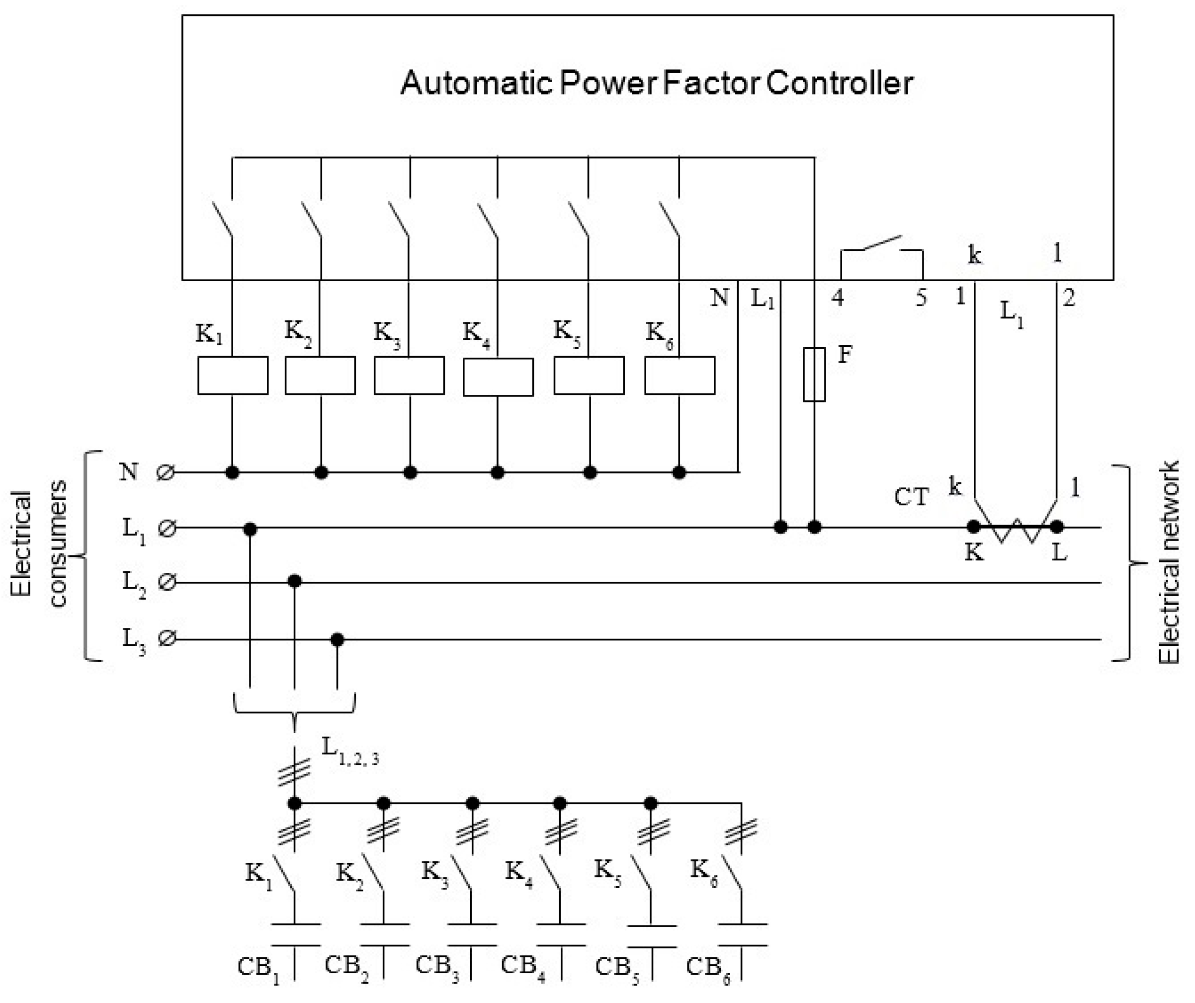
  • the current transformer is connected to the input terminals k and l, and the phase voltage of the L1 bar, to the terminals L1 and N of the APFC;
  • the first three outputs of the APFC are connected to the first three inputs of the first PLC, and the next three outputs to the first three inputs of the second PLC;
  • the first outputs of the two PLCs are connected to the command input of the three-phase power SSR, and the next six outputs of the two PLCs are connected to twelve EMCs, distributed six on each PLC;
  • the EMCs are divided into six groups, each group consisting of two EMCs, which together with the common three-phase SSR are part of the circuits of the six CBs, so that the first CB in the group has the main contacts in series with the execution element (thyristors in anti-parallel) of the three-phase SSR, and the main contacts of the second EMC short-circuit the series of execution elements of the previously mentioned contactors, directly supplying the CB from the power distribution bars.
The advantages are the following:
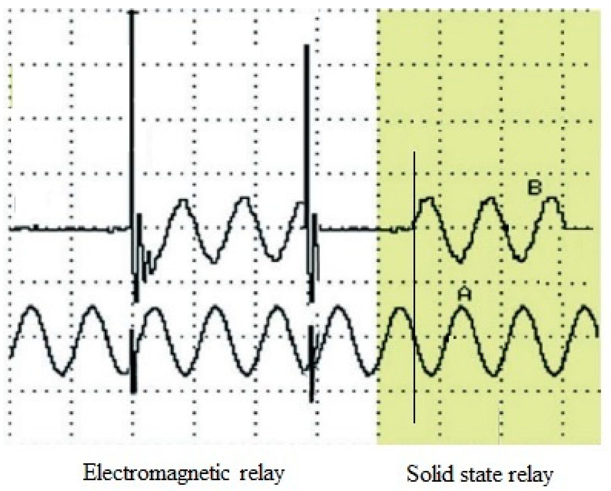
  • the currents when connecting the capacitors are much reduced (from (20–50)xIn to In, where In is the nominal current);
  • switch-on is performed at zero voltage;
  • there is no discharge in the arc when switching;
  • high reliability;
  • lower costs than in the case of using a three-phase SSR for each CB;
  • very high input/output isolation voltage;
  • does not generate disruptive electromagnetic fields;
  • superior lifetime compared to systems where CBs are connected with classical EMCs.
The presented method involves the use of PLCs (which must be programmed) that are controlled by a classic APFC, and when controlling a CB, two contactors are used instead of one.
The low-cost PF regulation system, reduction in transients, and elimination of the electric arc, with CBs, from three-phase low-voltage installations ensures, depending on the phase shift between voltage and current, a PF value around the imposed value (usually, neutral power factor 0.9), by properly connecting the CBs using a single three-phase power SSR.
The detailed scheme of the low-cost PF regulation installation with capacitors banks in three-phase low-voltage installations is presented in Figure 12. When the actual PF in the installation has such a value that to increase it to around the imposed value the APFC determines the activation of CB1, the APFC sets the logical value 1 of the output signal O1; in this case, also, the signal I1, from the input to PLC1, has the logical value 1. This value determines at the output of PLC1, after a short interval, the logical value 1 of the signal Q2. As a result, EMC K11 closes and its contacts close normally the capacitors bank circuit CB1; after the time t1 = 0.5 s the signal Q1 has the logical value 1 on the control input A of the three-phase power SSR, when the voltage crosses zero, so it switches on, and capacitors bank CB1 is connected to bars L1,2,3. After the time interval t2 = 0.5 s, the output signal Q3 has the logical value 1 and closes the EMC K12 (bypass EMC) which short-circuits the execution elements of the switching devices K and K11, connected in series, and supplies directly, from the bars L1,2,3, capacitors bank CB1. Now the three switching devices K, K11 and K12 are switched on. After time t3 = 0.5 s, signals Q1 and Q2 have the logical value 0, switching off devices K and K11, capacitors bank CB1 being connected to the network only through contact K12. The capacitors bank CB1 will remain connected in the installation for a time interval t4 set by the APFC, which depends on the value at a given moment and the imposed value of PF in the installation. After time t4, the APFC imposes the logical value 0, when, according to its program, PLC1 sets the logical value 0 of the output signal Q3. EMC K12 triggers and capacitors bank CB1 is switched off from the power supply. In the same way, the low-cost system of automatic PF adjustment can activate two or more CBs in the same time interval, according to the actual value of the PF.

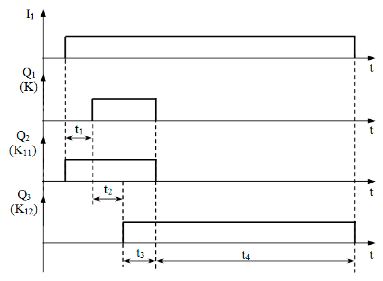
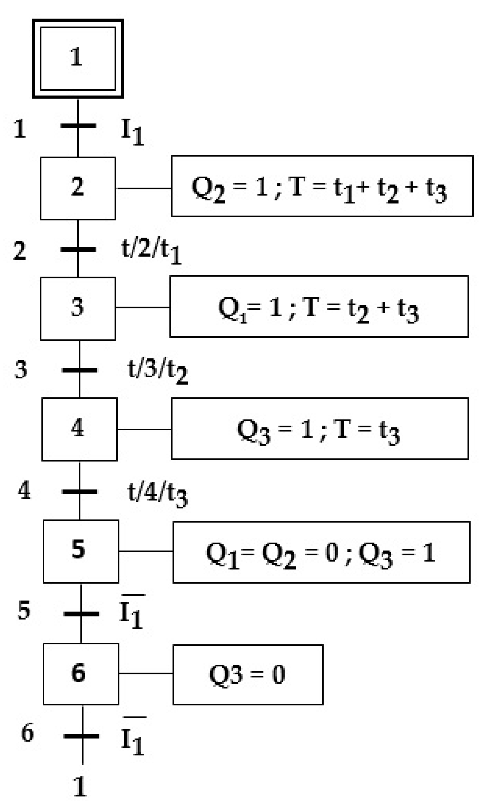
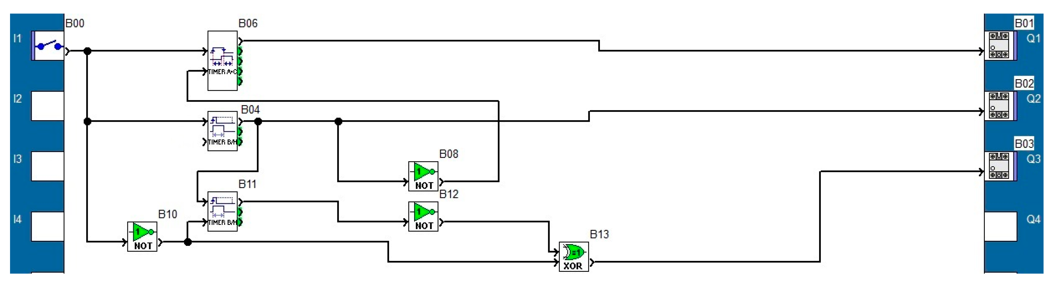
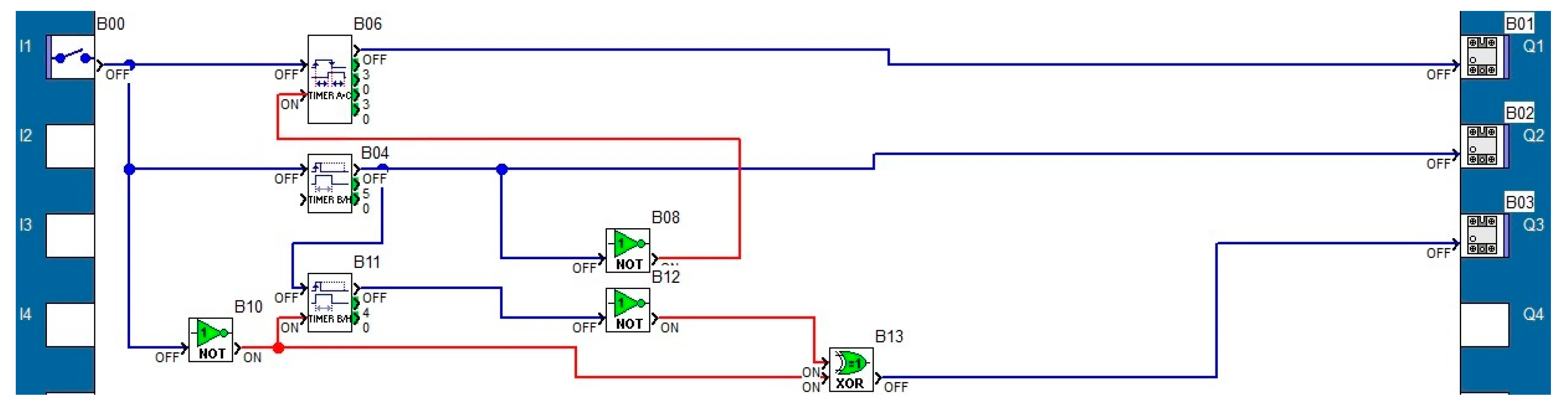
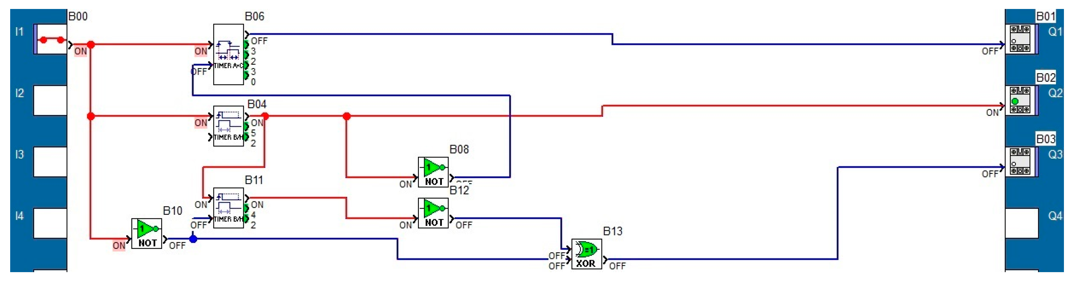
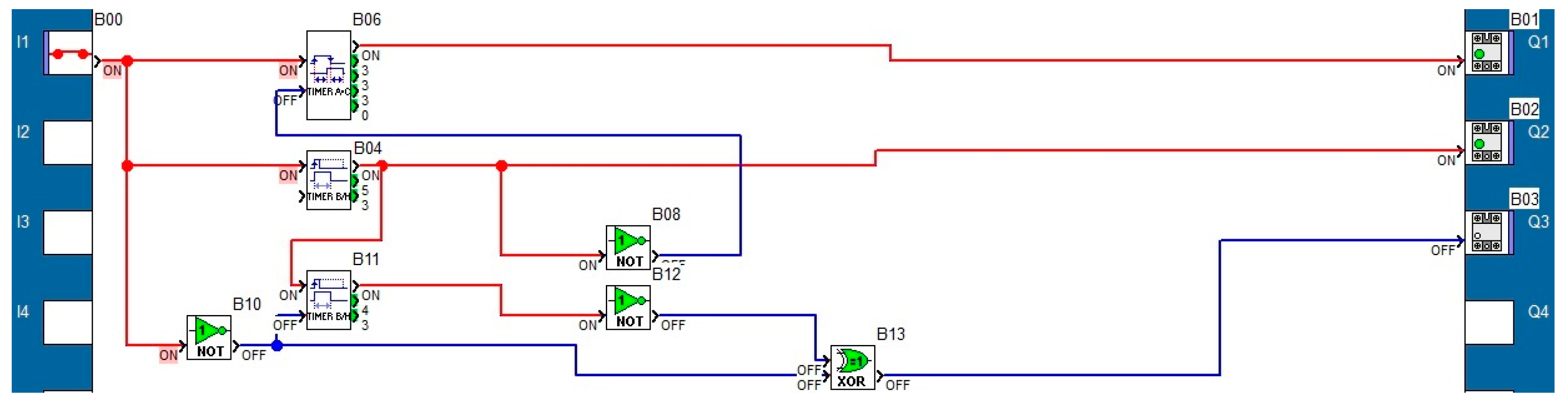
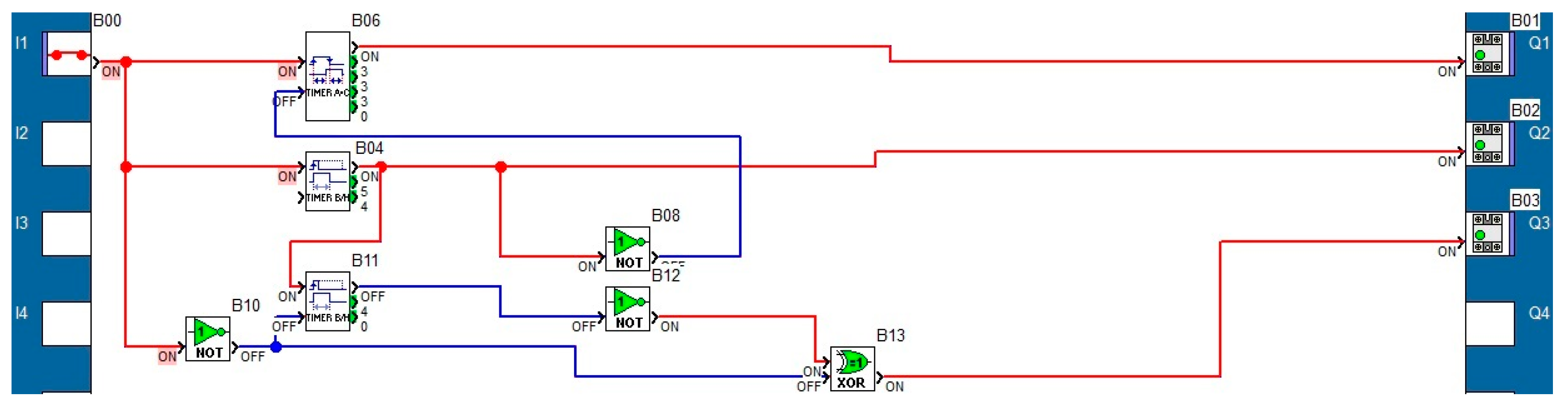
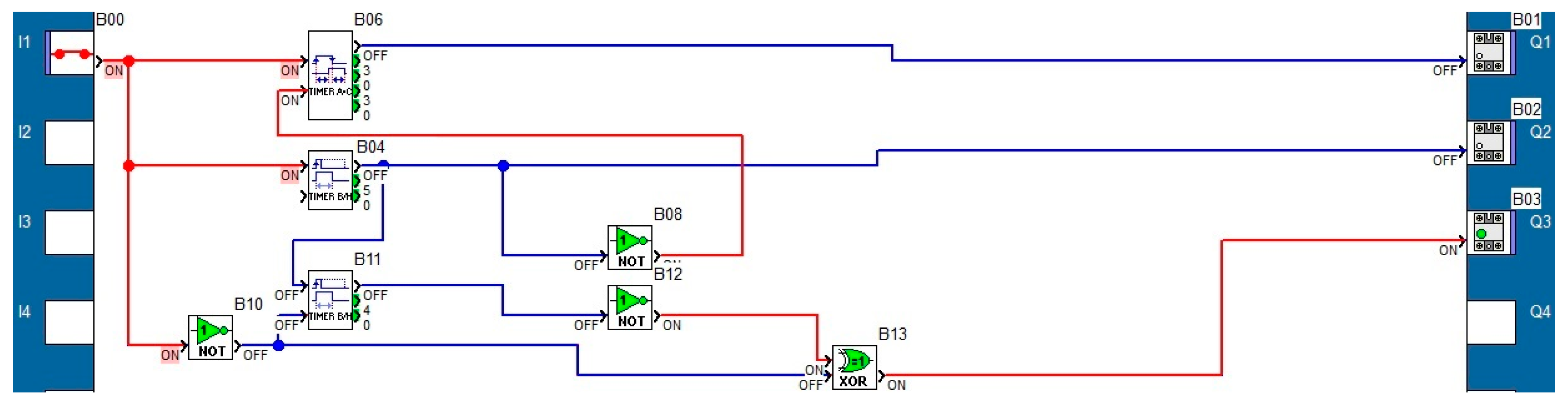
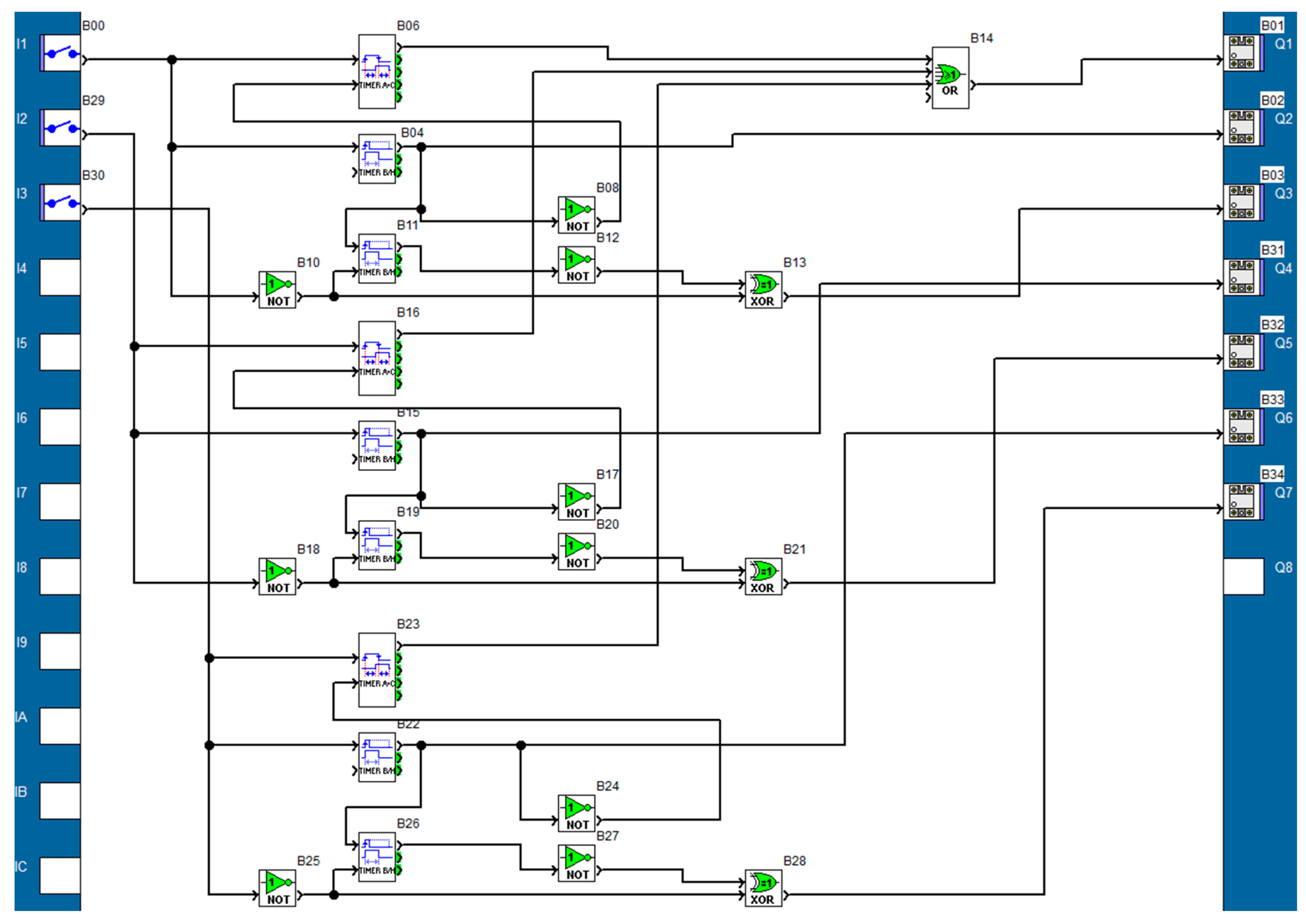
2.4. Programming the PLCs

In order to function, the PLCs in Figure 12 must have a program created in each PLC. Each SR2B201FU type PLC (Schneider; has 12 digital inputs, 1 logic is 24 V and 8 digital outputs, can be programmed in LAD—Ladder Diagram or in FBD—Function Block Diagram), can control three CBs (PLC1 controls CB1, CB2, CB3, and PLC2 controls CB4, CB5, CB6). In this way, three inputs of the automaton (I1–I3) and seven outputs (Q1–Q7) are used. The PLCs were programmed in FBD using Zelio Soft 2 (which can perform simulation, implementation, monitoring).
To create the program, the operation of the scheme in Figure 12 is used, where a time diagram (Figure 13) was created for the CB1 command.
Figure 13 shows the time variations of the signals I1, Q1, Q2, and Q3 that determine the connection and disconnection from the serviced installation of capacitors bank CB1. The same control logic established by the programs written in PLC1 and PLC2 is also used to connect CBs: CB2 (K, K21, K22 and PLC1 are used), CB3 (K, K31, K32 and PLC 1), CB4 (K, K41, K42 and PLC 2), CB5 (K, K51, K52 and PLC 2) and CB6 (K, K61, K62 and PLC 2).
Using the time diagram in Figure 13, the program graph in Figure 14 was built, which corresponds to the control of outputs Q1 (K, SSR), Q2 (K11) and Q3 (K12), on different time domains, if I1 = 1 (the APFC gave the command for connecting CB1). The connection of CB1 is timed by means of K, K11 and K12 when I1 = 1, and the disconnection of CB1 is instantaneous when I1 = 0. When implementing the program, the following times were used: t1= 0.5 s; t2 =0.5 s; t3 =0.5 s. The times were chosen to ensure a firm switching of EMCs and SSR.
Next, in Figure 15, Figure 16, Figure 17, Figure 18, Figure 19 and Figure 20, the operation of the program created for the control of CB1 is simulated. In principle, the program has three time relays: a time relay B06 with on-delay (t1) and off-delay (t2 + t3) used to control Q1 (K)—to reset B06, inverter B08 is used (from output B04); a time relay B04 of the monostable type (t1 + t2 + t3) which executes the command of Q2 (K11); a time relay B11 of the monostable type (t3 + t4), with inverted output, which performs the command of Q3 (K12)—to reset B11 the inverter B10 is used (from input I1). The XOR logic gate B13 is used so that the Q3 output becomes logical 0 if I1 goes from 1 to logical 0.
Figure 15 shows the program before running.
When running the program (Figure 16, Figure 17, Figure 18, Figure 19 and Figure 20), the signals that are in blue represent logical 0, and the signals that are in red are logical 1. If I1 = 0, it is observed that timers B06 and B11 are blocked (by Reset), timer B04 is not started, and outputs Q1–Q3 are at logical 0 (Figure 16).
If I1 = 1 (Figure 17), the timer B04 has a logical 1 at the output, the output Q2 = 1, and K11 is closing for the time interval t1 + t2 + t3 (Figure 13). During this time, the output of timer B11 is logical 1, and the output Q3 is logical 0.
After the passage of time t1, the output of timer B06 is logical 1, Q1 = logical 1, and K (SSR) enters in conduction (Figure 18), and CB1 is connected to the power supply (with minimal inrush current). Next, the output of timer B04 is logical 1 (K11 is closing). During this time, the output of timer B11 is logical 1, and the output Q3 is logical 0.
After the time interval t2 has passed, the output of timer B11 becomes logical 1, and the output Q3 becomes logical 1, K12 is closing. In this time interval t3, the three outputs (Q1, Q2, Q3) are logical 1 (Figure 19).
After the passage of the time interval t3, the outputs of the time relays B06 and B04 go to logical 0, and K and K12 trigger, CB1 being powered through the contactor K12, as long as I1 is logical 1 (Figure 20).
If I1 is logical 0 (command from APFC), the outputs of timers B06, B04 and B11 will be logical 0, outputs Q1, Q2, Q3 will be logical 0, and K, K11 and K12 will be triggered.
As mentioned, a PLC controls three CBs (e.g., PLC1 controls CB1, CB2, CB3). The program created for the control of the three CBs is presented in Figure 21. A logical OR gate (B 14) was also introduced that controls the Q1 (K) output. Otherwise, for the control of CB2 (through Q1, Q4, Q5) and CB3 (through Q1, Q6, Q7), the structure is the same as for the control of CB1.

2.5. Economical Review of Low-Cost APFC

An economic analysis is made to determine if the scheme from Figure 12 (which is the object of the work) is cheaper compared to the one from Figure 9. The two schemes (from Figure 9 and Figure 12) were chosen because they perform the same function (the classic scheme in Figure 8 connects the CBs without reducing the inrush current, so it cannot be compared with the other two schemes), namely switching the CBs through SSRs (so that the inrush current is minimal).
The following prices are taken into account for the equipment used in Figure 9 and Figure 12: APLC = EUR 600; PLC = EUR 90; SSR = EUR 130; EMC = EUR 20; Heatsink (HS) for SSR = EUR 4; CB = EUR 50. In the economic calculation, the conductors and auxiliary components to the conductors were not taken into account. For simplification, it is considered that the same CB is used on each step.
A comparative analysis will be made for four situations: APFC with 3 CBs; APFC with 6 CBs; APFC with 9 CBs; APFC with 12 CBs (Table 2).
As can be seen from Table 2, it is found that a small number of CBs (3) determines a more expensive installation by 10.6% compared to the scheme in Figure 9. If more than six CBs are used, the installation in Figure 12 is cheaper compared to the one in Figure 9: by 17.6% for six CBs, by 19.59% for nine CBs, and by 22.57% for twelve CBs. Obviously, the higher the number of steps, the cheaper the installation in Figure 12.

3. Results

In order to analyze the connection of the capacitors banks, an experimental analysis was carried out of the connection of the capacitors and capacitors banks through classical electrical contact (from the contactor) and an SSR (Z type). Measurements were made with an APFC with capacitors banks (on the six steps) and with coils inserted with capacitors banks (on the six steps). The experimental measurements were made with a power quality analyzer (CA 8334 B, Chauvin Arnoux). In the following figures with measurements, the signal that approaches the sinusoidal form is the voltage applied to the capacitor, and the more distorted signal is the current through the capacitor.

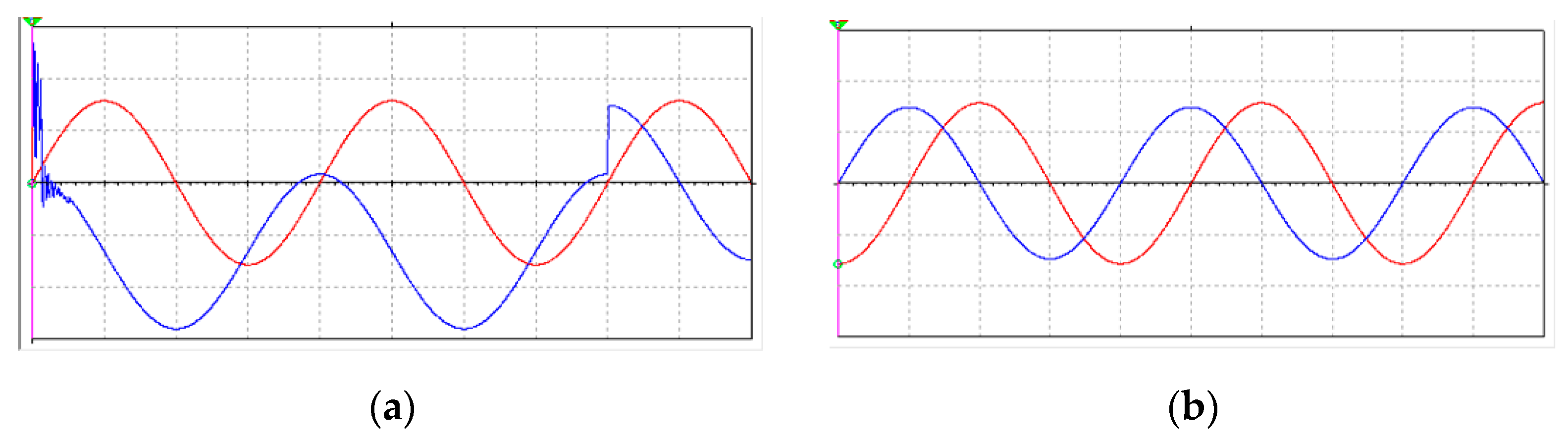
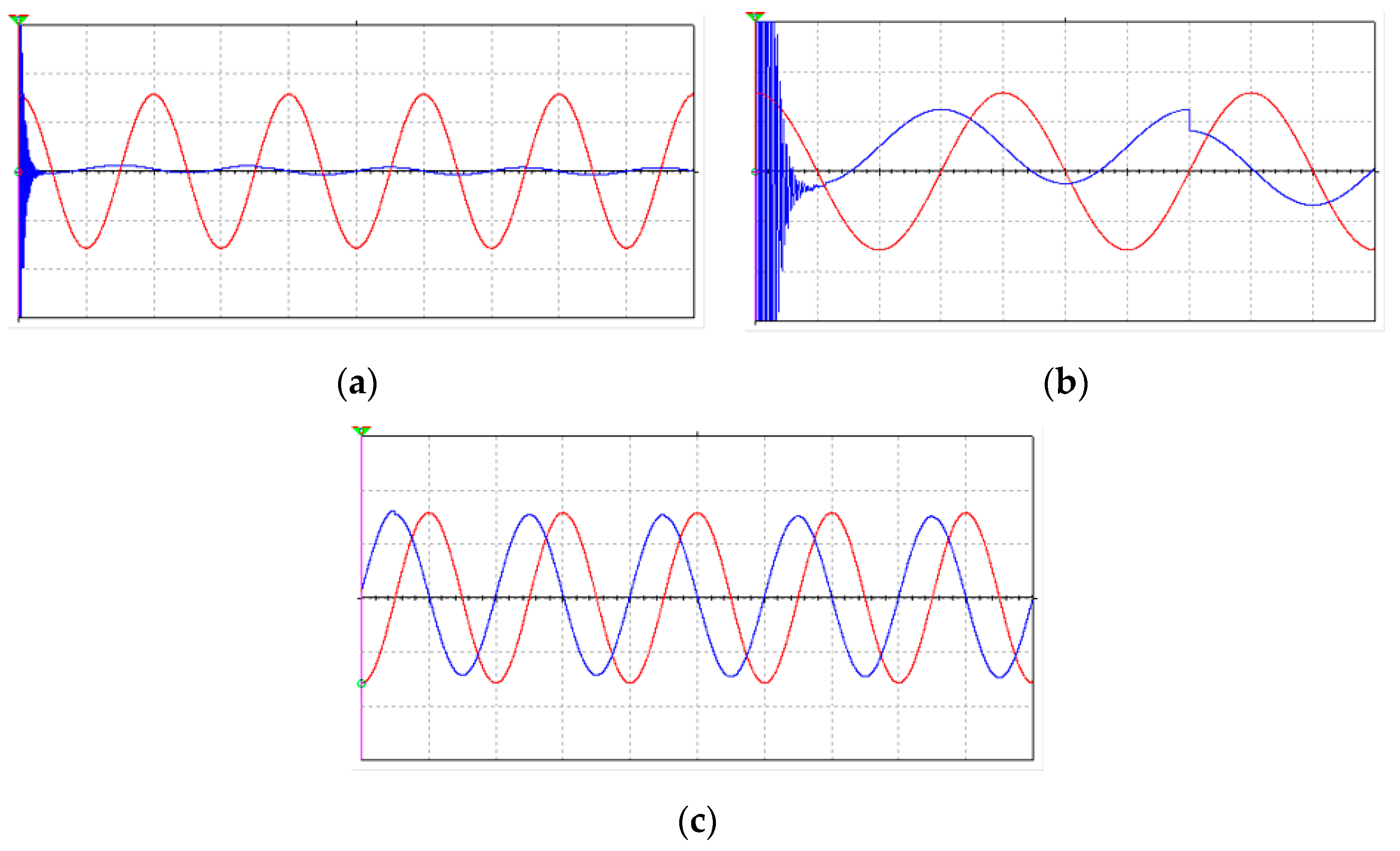
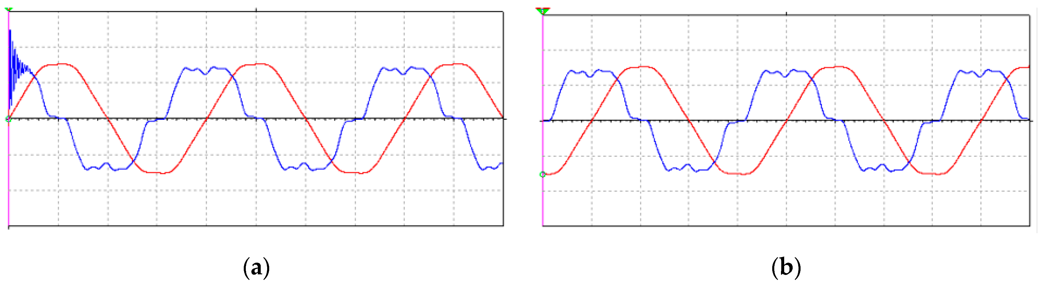
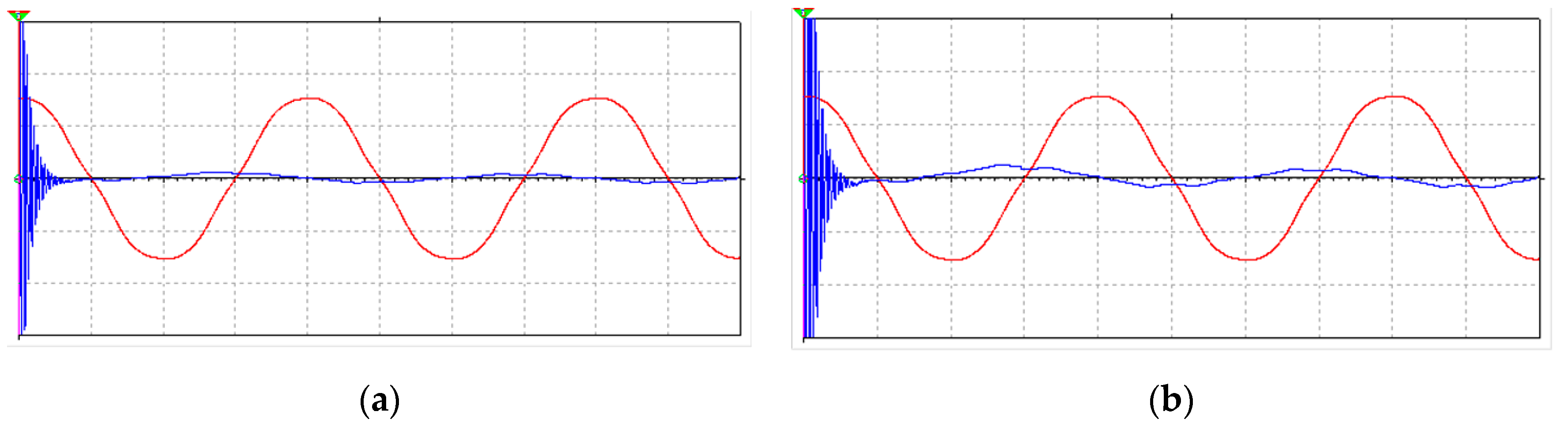
3.1. Connecting Capacitors and Capacitors Banks through Electrical Contacts and through Solid-State Relay

During the first experiments, an analysis was made on capacitors connected to single-phase voltage. In the following figures, THD is total harmonic distortion for current.
A 3.5 µF AC capacitor was connected through an electrical contact (classical) and the voltage, current (including at inrush) and harmonic spectrum were measured (Figure 22); then, a 15 µF AC capacitor was connected (Figure 23).
There are similarities between the simulations (Figure 6b and Figure 7) and experiments (Figure 22 and Figure 23). In the simulations and experiments, higher values were obtained for the inrush current (six to twenty times). In steady-state mode, similar values of the currents are obtained for simulations and measurements.
The capacitors are connected randomly at any value of the supply voltage (Figure 22a and Figure 23a). The higher the instantaneous voltage, the higher the inrush current will be (there may also be a transient voltage regime) and the electric arc will be more intense (with negative effects on the lifetime of the contactor contacts). Due to the operating principle of the capacitor, the current is before the voltage and is much more deformed than the voltage applied to the capacitor (Figure 22a,b and Figure 23a,b). In the spectrum of harmonics of the current (Figure 22c and Figure 23c) there are odd harmonics of order 5, 7, 9, 13.
A 3.5 µF AC and a 15 µF AC capacitor were connected, through a Z type single-phase SSR (zero-crossing command). Theoretically, it switches on the consumers when the voltage crosses zero, and switches off the consumers when the current crosses zero. The voltage, the current (including inrush) and the spectrum of harmonics were measured (Figure 24 and Figure 25). For the SSR (which replaces the EMC) to switch on, a command voltage of 5 V DC is applied.
When connected via SSR, the switching is performed at zero voltage, and the inrush current is the same as the usual current (Figure 24a,b and Figure 25a,b). In the first part of each period there are some spikes due to switching. And in the simulations, when the voltage passed through zero, small values were obtained for the inrush current (Figure 6a).
The capacitors are connected when the voltage on the capacitor is minimum (Figure 24a and Figure 25a), and the inrush current is lower than in the previous case. The current is more distorted (Figure 24b and Figure 25b) than in the previous case (THD higher by a few percent), the current harmonics (Figure 24c and Figure 25c) with ranks 5, 7, 9, 3, 13, 15 having higher values. So, a capacitor that is permanently supplied through an SSR leads to a larger distortion of the current. The importance of the SSR is when switching on the capacitor, when the inrush current is much reduced and the electric arc does not exist.
In Figure 26a, the currents were measured in steady-state mode through a CB powered by classical electrical contacts, and in Figure 26b through a three-phase SSR. The capacitors bank consists of three capacitors in a wye connection, each capacitor being 15 µF/450 V AC. The currents are more distorted when connecting the CB through the SSR.
In Figure 27a, the currents through a CB connected to a three-phase induction motor (IM) powered by classical electrical contacts were measured in steady-state mode, and in Figure 27b the currents through a CB connected to a three-phase induction motor (IM) powered by a three-phase SSR. The capacitors bank consists of three capacitors in a wye connection, each capacitor being 15 µF/450 V AC, and the three-phase induction motor (running at idle) has a power of 750 W; 1450 rpm; 400 V; 2.13 A; PF = 0.72. The currents are more distorted when the CB and IM are supplied through the SSR (Figure 27b).
When connecting CBs through SSRs with zero-crossing switching, inrush current is limited and in steady-state mode, the current is more distorted (thyristors connected to CBs are non-linear elements) compared to connecting through classic electrical contacts. So, when connecting CBs, it is useful to connect via SSR and when operating in steady-state mode the capacitors must be powered through classical electrical contacts that do not increase the deforming current.

3.2. Experiments with Three-Phase Capacitors Banks

A group of experiments was carried out with the APFC (Roederstein ESTAmat RPR type) from Figure 12. In Figure 12, the current transformer has the following data: 15/5 A, SM 5 VA, Metra type. Electrical consumers can be switched on/switched off with classical switches (S1, S2, and/or S3)—Figure 28.
The measurements in Section 3.2 and Section 3.3 were made on a single phase (L1) so that the signals are easier to visualize.
The following consumers were used in the experiments (Figure 12):
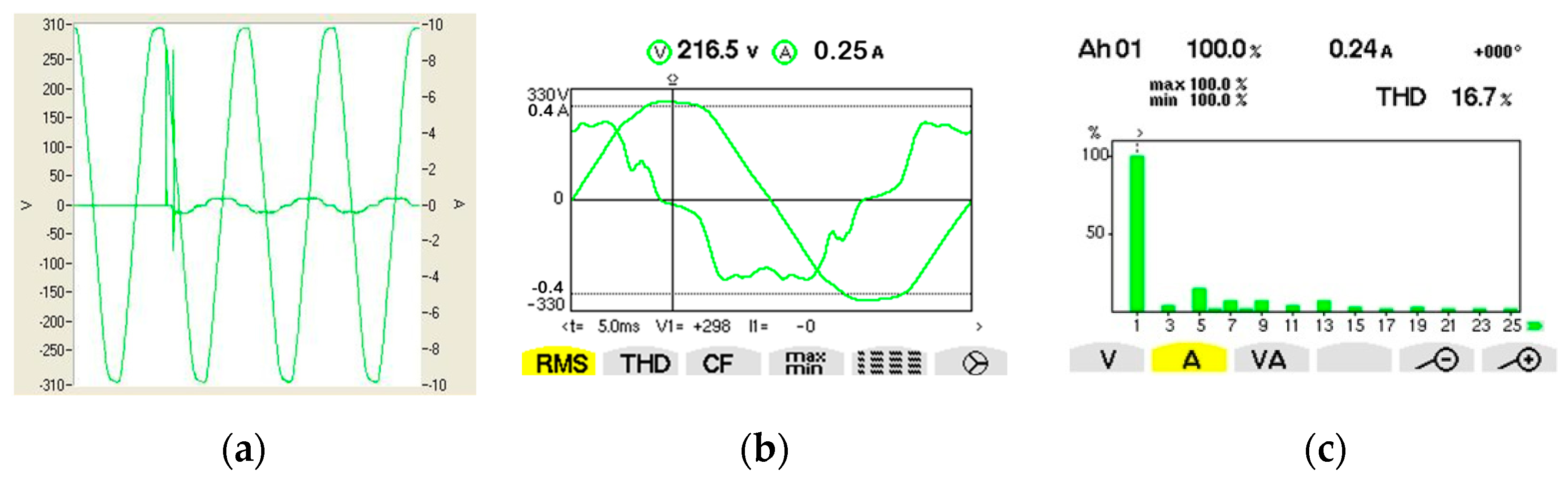
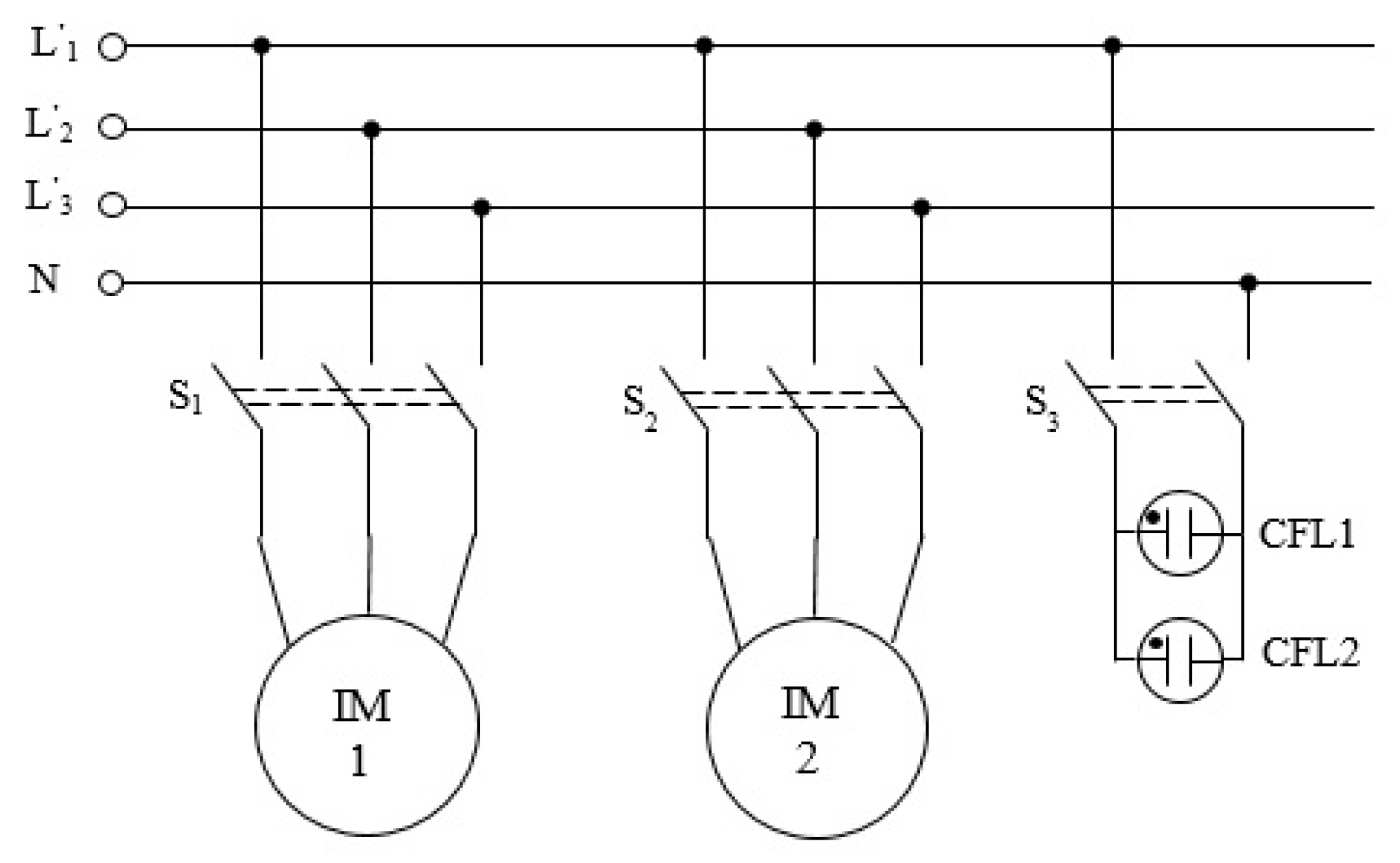
  • M1, three-phase induction motor (Figure 29) with the following data (ASI 90L-24-2 type): 2.2 kW; 2780 rpm; 400 V; 4.95 A; PF = 0.855;
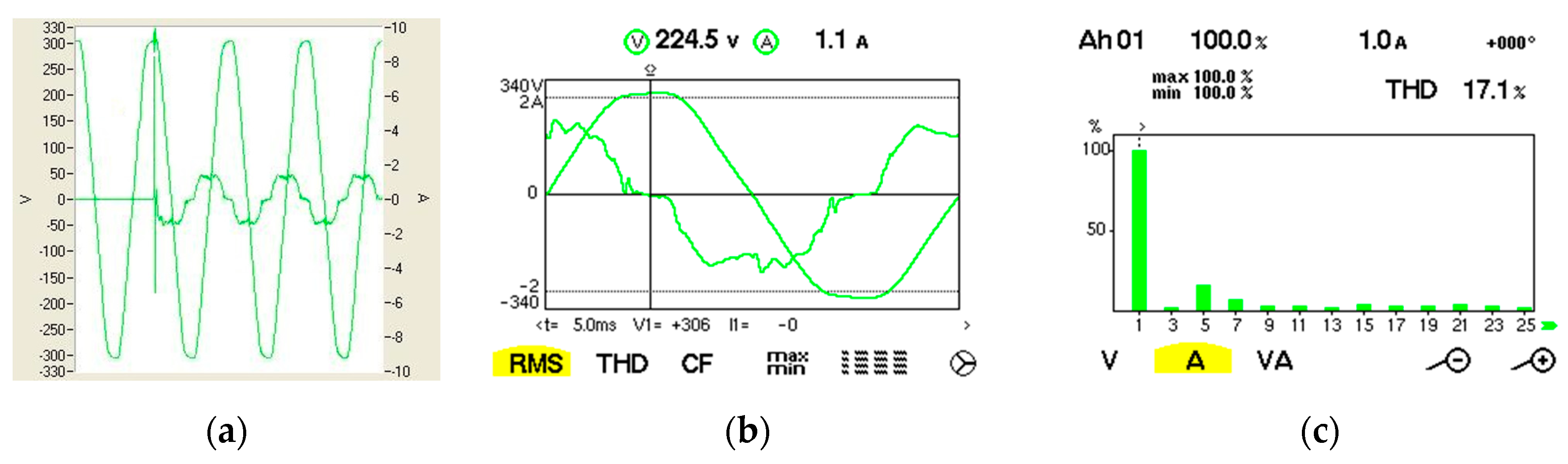
  • M2, three-phase induction motor (Figure 30) with the following data (N 80 L type): 750 W; 1450 rpm; 400 V; 2.13 A; PF = 0.72;
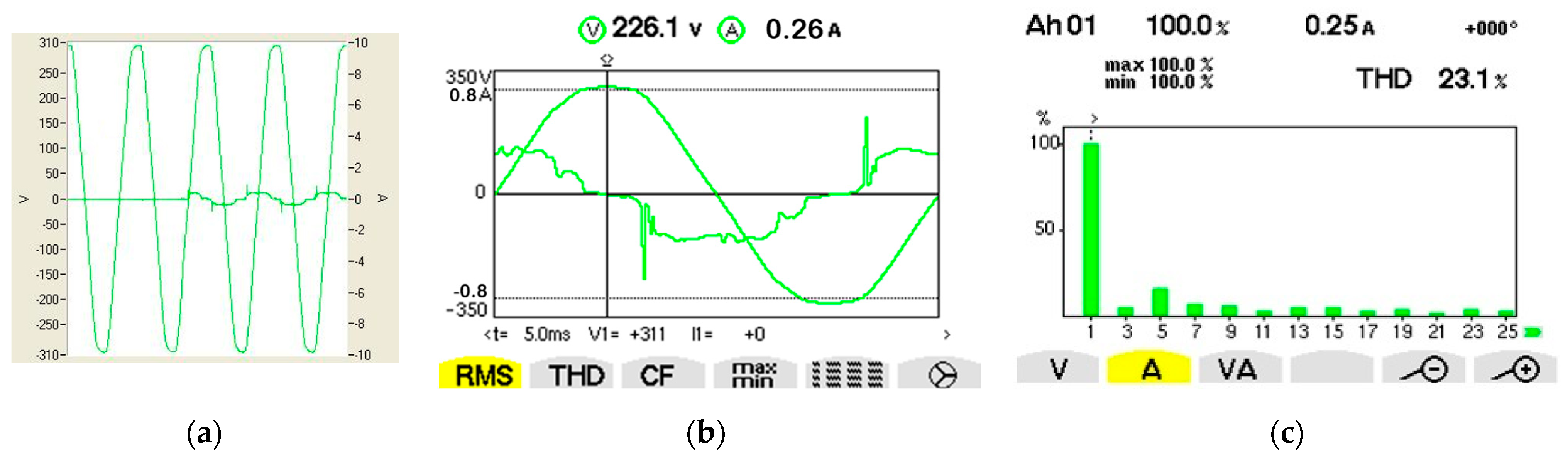
  • Compact fluorescent lamps (Figure 31), connected in parallel on the phase, with the following data: CFL1: 220 V, 50 Hz, 85 W, 6400 K; CFL2: 220–240 V, 50/60 Hz, 120 W, 580 mA, 4000 K.
Voltage and current were measured (Figure 29, Figure 30 and Figure 31), as well as the spectrum of current harmonics for each group of consumers.
The electric motors (M1, M2) worked at idle (without mechanical load), in order to have a PF as low as possible (for the APFC to introduce CBs). In the following experiments, to simplify, the measurements in the figures below were made on a single phase. Experiments were made with electrical installations from Figure 12 and Figure 28. The steady-state measurements were presented, after the CBs were connected through the electrical contacts of the EMCs (explanations in Figure 12).
Six CBs and three electrical consumers were connected to the APFC in Figure 12 (two three-phase IMs and two CFLs connected in parallel between one phase and neutral—Figure 12). The steps of CBs, in wye connections, have the following capacitors (on each branch of the wye connection): Step 1: C1 = 4 µF/450 V AC; Step 2: C2 = 5 µF/450 V AC; Step 3: C3 = 11.9 µF/450 V AC; Step 4: C4 = 16.9 µF/450 V AC; Step 5: C5 = 7.5 µF/450 V AC; Step 6: C6 = 10 µF/450 V AC. The reactive powers of the CBs were chosen so that, if all the consumers are connected to power supply, a PF above 0.9 can be achieved. During the operation of the APFC, delays are made when switching on and switching off the CBs.
The following experiments (Figure 32, Figure 33, Figure 34, Figure 35 and Figure 36) were carried out with CBs (of different values) connected in wye on each step (1 to 6, Figure 12).
Initially, the induction motor M1 (PF = 0.11) was connected, which worked at idle. To start the APFC, an electric consumer must be connected (minimum current of over 150 mA through secondary of CT, to be notified by the APFC). At the beginning, the identification cycle is carried out (three times, approx. in 3 min) by the APFC of the CBs connected on each step (to check their presence, their value, possibly their unbalance).
After checking the CBs, the measurements made for the M1 motor are shown in Figure 32. An important phase shift between voltage and current is observed (the character of the motor being inductive), and the current has a larger amplitude and is slightly distorted (a bit more distorted compared to the voltage).
Next, experimental measurements are presented after the three-phase SSR connection was made (according to the operating logic shown in Figure 12).
After a period of time, steps 3, 4 and 5 were connected (Figure 33). The phase shift between the fundamental current and voltage becomes smaller, the amplitude of the current decreases, but the current is deformed (it deviates more from the sinusoidal form).
Then the induction motor M2 was connected. After a period of time, the APFC automatically connected steps 1, 2 and 3 (all steps were connected)—Figure 34. The current increases (more consumers were introduced), but it is more distorted.
Next, CFLs were connected (they have a capacitive character and non-linear). After a period of time, step 1 was disconnected, the other steps being connected.
The APFC tried another combination of steps (CBs). It disconnected step 2 and reconnected step 1. Thus, steps 1, 3–6 remained connected (Figure 36), the resulting current being smaller, but equally distorted.

3.3. Experiments with AC Reactors Connected in Series with Three-Phase Capacitors Banks

The following experiments (Figure 37, Figure 38, Figure 39 and Figure 40) were carried out with capacitors banks (of different values) wye connected, each phase of the coils being connected with one coil (to realize the filtering function). The coils, connected on each step, have the following values: Step 1: L1 = 47 mH; Step 2: L2 = 47 mH; Step 3: L3 = 15.5 mH; Step 4: L4 = 26.42 mH; Step 5: L5 = 10.81 mH; Step 6: L6 = 97 mH. In principle, the coils were thus chosen to perform the filtering of current harmonics. The capacitors (from CBs) have the same values as those presented in Section 3.2.
Initially, the induction motor M1 (PF = 0.11) was connected, which worked at idle. After completing the identification cycle (approx. 3 min) by the APFC of the CBs connected on each step, and after a further period of time, steps 2, 3 and 4 were introduced, and the experimental measurements are presented in Figure 37. The phase shift between voltage and current and the current decrease, but the current is more distorted.
Then, the induction motor M2 was connected. After a period of time, the APFC automatically connected steps 2–6 (all steps were connected)—Figure 38. The current increases (more consumers were introduced) and is less distorted.
Next, CFLs were connected (they have a capacitive character). After a period of time, step 1 was disconnected, the other steps being connected (Figure 39).
By connecting CFLs, the current distorted even less. The highest harmonics are 5, 3, 7, 9.
After a period of time, the CFLs were disconnected and for a short period of time steps 1, 2, 4, 5, 6 were kept connected automatically. The voltage, current and harmonic spectrum were measured in Figure 40.
When using AC reactors connected in series with CBs, under the same operating conditions, the currents are less distorted (for THD lower values from a few percent to tens of percent), but have bigger values. In this way, the deforming effect of the capacitors on the currents is reduced.

4. Discussion

In electrical engineering, the importance of maintaining a high PF in low-voltage electrical installations is known. An APFC with three-phase CBs (which can be timed to switch on/switch off) is mounted at the point of common coupling (e.g., secondary windings of power transformer from power substations) in order to obtain a higher PF (than the neutral PF). Usually, CBs are connected through EMCs (at start-up, important transients occur when they are connected with negative effects on the life of the electrical contacts; switching is performed randomly, there is the possibility of connection when the voltage is maximum) or with SSRs (e.g., Z type, transients are reduced when connecting the CBs; the connection can be made at zero voltage, and the disconnection at zero current, but they are expensive).
The AC power capacitor does not always comply with the rated current and voltage specifications. Thus, EMCs contacts are always sufficiently large in terms of current and expected current, and the load should be equipped with additional circuits depending on its behavior (e.g., whether the load is, generally, capacitance, filters, switches or induction, solenoid and electric motors). If a capacitance or inductive load lacks appropriate restriction circuits, it can easily damage or destroy the EMC or control device incorporated.
Even with a small value capacitor, the input current can reach tens of amps for a short period of time from hundreds of µs to ms. Since the current quickly drops to the later evaluation value, the inrush current is not significant from a long-term perspective. However, it is possible to observe the effect when switching on power capacitors connected to an undersized circuit breaker: when the device is turned on, the circuit breaker automatically often switches off. Ideally, the maximum switching current of the EMC contact should be close to the specified input current, or the input current should be limited.
This paper does not have as its object the improvement of the deforming regime through the use of harmonic filters and no simulations were performed with an SSR for capacitive loads (difficult control). The purpose of the work is to analyze the operation of the APFC proposed in Figure 12.
The low-cost APFC system with CBs in three-phase low-voltage installations can also be achieved with other numbers of CBs. If three CBs are used, an APFC, a PLC (proposed models), a three-phase power SSR and six EMCs are used. For the diagram in Figure 12, depending on the number of PLC outputs, a PLC with several outputs, a PLC and extension module, or two or more PLCs can be used to control the CBs.
The APFC installation is low-cost because it uses a single three-phase SSR K (an expensive device; Figure 12) that switches on, according to the programs from PLC1 and PLC2, the six CBs (for each CB is used one SSR and two EMCs). By using the connection of CBs through SSR, the transients when switching on CBs are considerably reduced, and the electric arc does not exist when switching on CBs. At the same time, to reduce the deforming regime, the proposed APFC supplies the CBs in a steady-state regime through classical electrical contacts. As it was found, the use of a Z type SSR when connecting CBs, which have two thyristors (non-linear circuit elements) in steady-state mode, leads to greater current distortion. It is not recommended to supply CBs through an SSR (Z type) for long periods of time.
From the point of view of the costs of the APFC installation, in principle, if a minimum number of three CBs is used, with the increase in the number of controlled CBs, the installation from Figure 12 becomes increasingly cheaper than the one in Figure 9. If six, nine or twelve CBs are used, the installation from Figure 14 is 17.6%, 19.59%, or 22.57% cheaper than the installation from Figure 9.

5. Conclusions

In industrial applications in the power industry, it is important to maintain a power factor as high as possible (higher than the neutral power factor) at the point of common coupling (in power substations at the power transformer on the low voltage) for as long as possible.
An efficient method is (a well-known method) to use an automatic power factor controller which, depending on the phase shift between current and voltage (usually, on a single phase), switches capacitors banks (whose value and number depend on the application) connected through electromagnetic contactors (which have classical electrical contacts). By switching on the capacitors banks, the electrical contacts will be extremely stressed. When connected, an important electric arc appears and an inrush current that can be tens of times higher than the nominal current. The value of the inrush current depends on the current value of the applied voltage and the initial voltage on the capacitors. Currently, in order to reduce the inrush currents and to improve the deforming regime of the currents, capacitors banks are inserted with coils (which also have the function of harmonic filters).
Solid-state relays (e.g., Z type) can be used in the transient mode when connecting the capacitors banks because there is no longer an electric arc and the inrush current is greatly reduced. Due to the non-linear character of solid-state relays, in steady-state mode the capacitors banks must be supplied through classical electrical contacts in order not to distort the currents even more. Because three-phase solid-state relays are expensive components, the proposed solution for the automatic power factor controller uses a single three-phase solid-state relay and several electromagnetic contactors (two for each capacitors bank, instead of one as in the classical connection solution). In this way, it can achieve a cheaper automatic power factor controller (by tens of percent) compared to the classical automatic power factor controller.
The novel elements brought by the proposed method are:
  • The realization principle of the power improvement installation with an automatic power factor controller with PLCs (one or more depending on the constructive type and the number of capacitors banks), electromagnetic contactors (two for each capacitors bank) and a three-phase SSR used to connect all the capacitors banks;
  • The electrical power scheme, composed of two electromagnetic contactors, for each individual capacitors bank and a single three-phase SSR, used to connect all capacitors banks;
  • The program implemented on the PLC for the control of the capacitors banks, so as to realize the switch-on at zero voltage of the capacitors banks.
According to the proposed scheme, a three-phase solid-state relay and two contactors (three-phase) are used when connecting (in transient mode) a capacitors bank. In steady-state mode, the capacitors bank is powered by a single contactor. Because it works for a short period of time, the other contactor can be of lower power (to make the installation as cheap as possible). Future research will be carried out in this direction. Further research will be carried out to simulate the voltage and current when connecting real capacitors through an SSR (difficult control) to non-sinusoidal voltage sources.

6. Patents

The paper is based on patent application no. A 2020 00491 from 4 August 2020 submitted to the State Office for Inventions and Trademarks, Romania. The title of the patent application is: “Economic system for automatic adjustment of the power factor, with capacitors banks, from three-phase low-voltage installations”, authors Gabriel Nicolae Popa, Corina Maria Diniș, Iosif Popa.

Author Contributions

Conceptualization G.N.P.; Data curation, C.M.D. and G.N.P.; Formal analysis, G.N.P. and C.M.D.; Investigation, G.N.P.; Methodology, C.M.D. and G.N.P.; Supervision, G.N.P.; Writing—G.N.P. All authors have read and agreed to the published version of the manuscript.

Funding

This paper benefited from financial support through the program on “Supporting the research activity by funding an internal grant competition—SACER 2023”, Competition 2022, University Politehnica Timișoara, Financing contract no.28/03.01.2023.

Data Availability Statement

Data are contained within the article.

Acknowledgments

The authors bring gratitude to the beautiful collaboration with Iosif Popa, who passed away in 2023.

Conflicts of Interest

The authors declare no conflicts of interest.

References

  1. Power Factor Correction and Harmonic Filtering in Electrical Plants; Technical Application Papers No. 8 ABB; Electrical Engineering Portal: Belgrade, Serbia, 2010.
  2. Power Factor Correction and Control of Electrical Network Quality. ALPES Technologies. Available online: https://www.alpestechnologies.com/sites/all/images/pdf_EN/EX216012_AT_EN_BD.pdf (accessed on 19 January 2024).
  3. Power Factor Correction: A Guide for the Plant Engineer; Technical Data SA02607001E; EATON: Hampton, UK, 2022.
  4. Voloh, I.; Ernst, T. Review of Capacitor Bank Control Practices; GE Grid Solutions: Shanghai, China, 2015. [Google Scholar]
  5. Reactive Power Compensation, ABB, Santiago, Chile. 5 June 2013. Available online: https://new.abb.com/docs/librariesprovider78/chile-documentos/jornadas-tecnicas-2013---presentaciones/4-jos%C3%A9-matias---reactive-power-compensation.pdf?sfvrsn=2 (accessed on 18 January 2024).
  6. Riese, P. Manual of Power Factor Correction; FRAKO: Teningen, Germany, 2010. [Google Scholar]
  7. Koomey, J.G. Assessment of the Impacts of Power Factor Correction in Computer Power Supplies on Commercial Building Line Losses; Lawrence Berkeley National Laboratory: Berkeley, CA, USA, 2006.
  8. Solid State Relays Common Precautions; OMRON: Tokio, Japan, 2010. Available online: https://omronfs.omron.com/en_US/ecb/products/pdf/precautions_ssr.pdf (accessed on 15 January 2024).
  9. Solid State Relays; Application Note AP04901001E; EATON: Hampton, UK, 2019.
  10. Tasker, A. Considerations for Design Using Radiation Hardened Solid State Relays; Application Note AN-1068; International Rectifier: Los Angeles, CA, USA, 2015. [Google Scholar]
  11. Ramos, R. Film capacitor in power applications. IEEE Power Electron. 2018, 5, 45–50. [Google Scholar] [CrossRef]
  12. Latt, A.Z. Power Factor Correction Using Shunt Capacitor Bank for 33/11/0.4 kV, 10 MVA Distribution Substation. Int. J. Innov. Res. Multidiscip. Field 2019, 5, 1–8. [Google Scholar]
  13. Tan, M.; Zhang, C.; Chen, B. Size Estimation of Bulk Capacitor Removal Using Limited Power Quality Monitors in the Distribution Network. Sustainability 2022, 14, 15153. [Google Scholar] [CrossRef]
  14. Power Quality Application Guide. Available online: https://www.sier.ro/ghid_aplicare.html (accessed on 24 February 2024).
  15. Thentral, T.M.T.; Usha, S.; Palanisamy, R.; Geetha, A.; Alkhudaydi, A.M.; Sharma, N.K.; Bajaj, M.; Ghoneim, S.S.M.; Shouran, M.; Kamel, S. An energy efficient modified passive power filter for power quality enhancement in electric drives. Front. Energy Res. 2022, 10, 989857. [Google Scholar] [CrossRef]
  16. Sa’ed, J.A.; Amer, M.; Bodair, A.; Baransi, A.; Favuzza, S.; Zizzo, G. A Simplified Analytical Approach for Optimal Planning of Distributed Generation in Electrical Distribution Networks. Appl. Sci. 2019, 9, 5446. [Google Scholar] [CrossRef]
  17. Scott, M.A. Working safely with hazardous capacitors. IEEE Ind. Appl. Mag. 2019, 25, 44–53. [Google Scholar] [CrossRef]
  18. Raghavendra, P.; Dattatraya, N.G. Coordinated volt-var control. IEEE Ind. Appl. Mag. 2018, 24, 14–22. [Google Scholar] [CrossRef]
  19. Ye, J.; Gooi, H.B. Phase Angle Control Based Three-phase DVR with Power Factor Correction at Point of Common Coupling. J. Mod. Power Syst. Clean Energy 2020, 8, 179–186. [Google Scholar] [CrossRef]
  20. Helmi, B.A.; D’Souza, M.; Bolz, B.A. Power factor correction capacitors. IEEE Ind. Appl. Mag. 2015, 21, 78–84. [Google Scholar] [CrossRef]
  21. Tariq, H.; Czapp, S.; Tariq, S.; Cheema, K.M.; Hussain, A.; Milyani, A.H.; Alghamdi, S.; Elbarbary, Z.M.S. Comparative Analysis of Reactive Power Compensation Devices in a Real Electric Substation. Energies 2022, 15, 4453. [Google Scholar] [CrossRef]
  22. Ahmed, M.A. Point of Common Coupling Power Factor Conditioning of Connected Loads with PWM Rectifier. WSEAS Trans. Power Syst. 2019, 14, 24–32. [Google Scholar]
  23. Rahimi, S.; Marinelli, M.; Silvestro, F. Evaluation of Requirements for Volt/Var Control and Optimization Function in Distribution Management Systems. In Proceedings of the 2nd IEEE ENERGYCON Conference and Exhibition, Florence, Italy, 9–12 September 2012; pp. 331–336. [Google Scholar] [CrossRef]
  24. Gupta, A.G.; Yadav, O.P.; DeVoto, D.; Major, J. A Review of Degradation Behavior and Modelling of Capacitors. In Proceedings of the ASME 2018 International Technical Conference and Exhibition on Packaging and Integration of Electronic and Photonic Microsystems, San Francisco, CA, USA, 27–30 August 2018; pp. 1–10. [Google Scholar] [CrossRef]
  25. Popa, G.N.; Dinis, C.M.; Popa, I. Economical System for Automatic Power Factor Adjustment, with Capacitors Banks, in Three-Phase Low-Voltage Installations. Patent no. A 2020 00491, 4 August 2020. (In Romanian). [Google Scholar]
  26. Coman, C.M.; Florescu, A.; Oancea, C.D. Improving the Efficiency and Sustainability of Power Systems Using Distributed Power Factor Correction Methods. Sustainability 2020, 12, 3134. [Google Scholar] [CrossRef]
  27. Stosur, M.; Sowa, K.; Kuczek, T.; Chmielewski, T.; Ruszczyk, A.; Koska, K. Overvoltage Protection of Solid State Switch for Low Voltage Applications–Simulation and Experimental Results. In Proceedings of the European EMTP-ATP Conference, Kiel, Germany, 4–6 September 2017; pp. 1–10. Available online: https://www.researchgate.net/profile/Kacper-Sowa/publication/319543888_Overvoltage_protection_of_solid_state_switch_for_low_voltage_applications_-_simulation_and_experimental_results/links/59b26e47a6fdcc3f8891c6ec/Overvoltage-protection-of-solid-state-switch-for-low-voltage-applications-simulation-and-experimental-results.pdf (accessed on 20 January 2024).
  28. Ruszczyk, A.; Janisz, K.; Koska, K. Solid-State Switch for Capacitors Bank Used in Reactive Power Compensation. In Proceedings of the XII International School on Nonsinusoidal Currents and Compensation, ISNCC 2015, Łagów, Poland, 15–18 June 2015; pp. 1–5. [Google Scholar]
  29. Technical Explanation of Solid State Relays; CSM_SSR_TG_E_9_2; OMRON: Tokio, Japan, 2018.
  30. From Electromechanical Relays to Robust Semiconductor Solutions: Solid-State Relays with Optimized Superjunction FET Technology; Infineon Technology: Richardson, TX, USA, 2021.
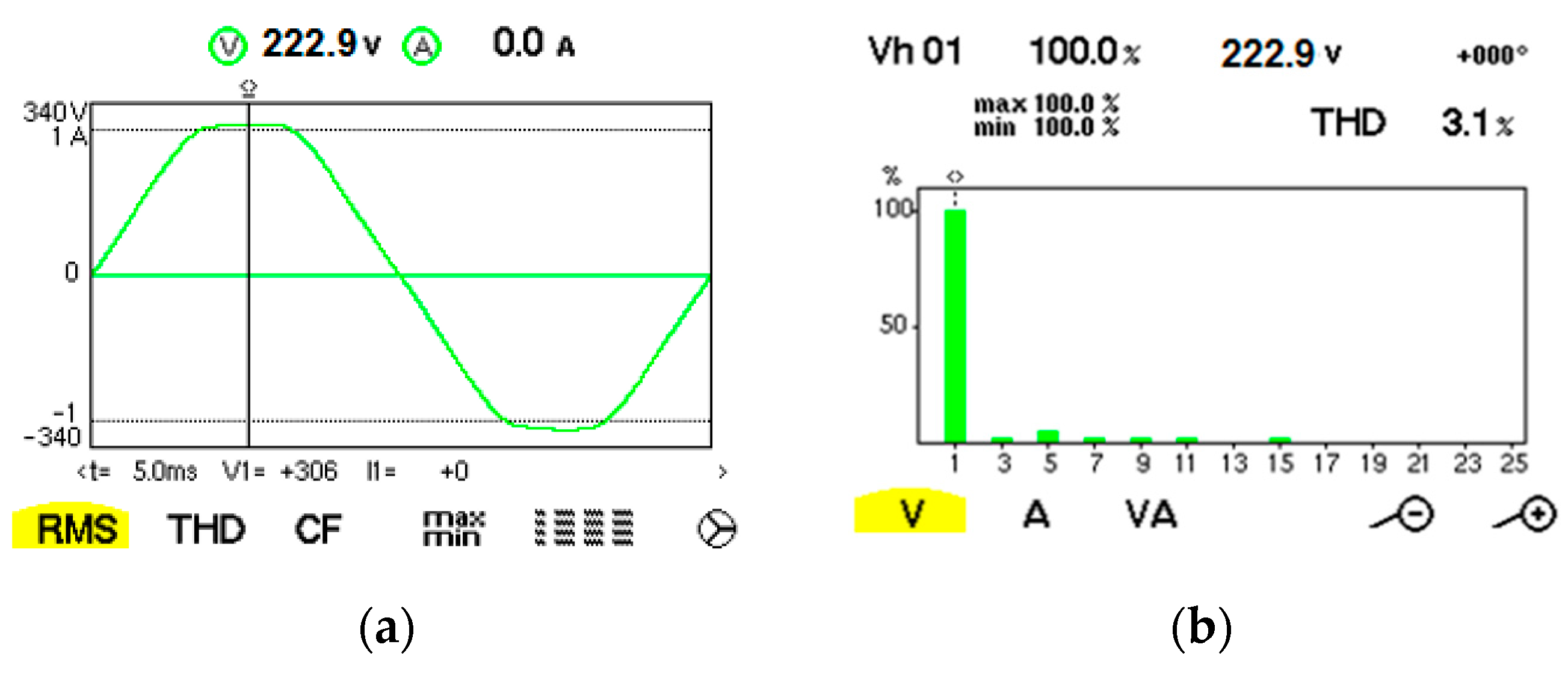
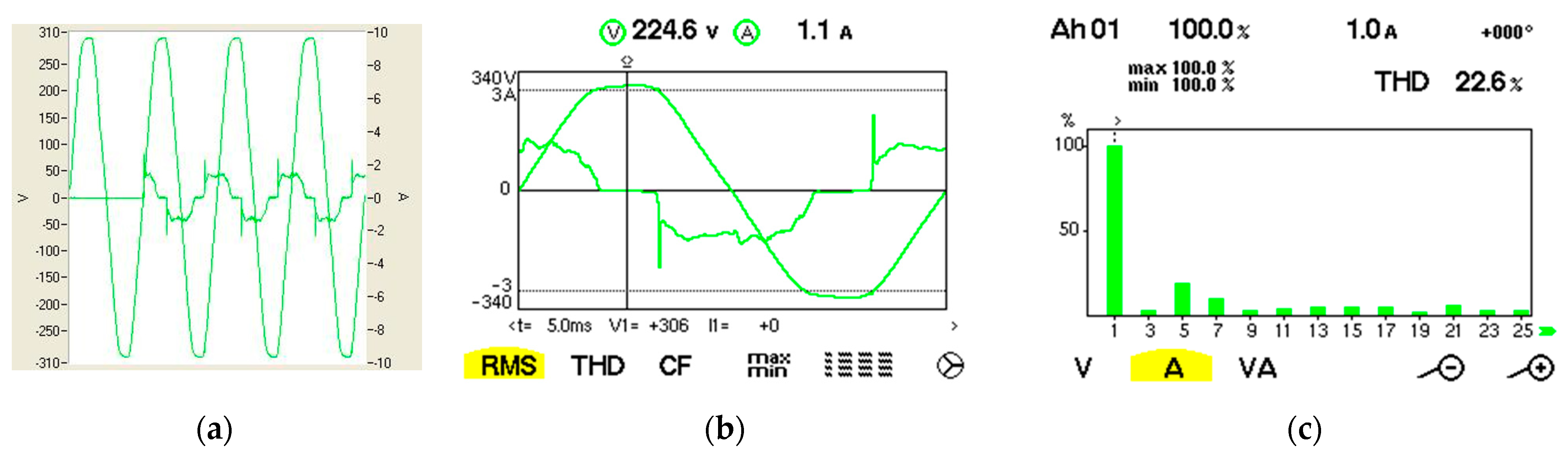
Figure 1. Simulation with the voltage (red) and current (blue) through an ideal capacitor of 15 µF connected at the sinusoidal voltage 222.91 V, RMS (current shifted by 90° before the voltage).
Energies 17 01363 g001
Figure 2. The electrical model for the real capacitor.
Energies 17 01363 g002
Figure 3. (a) Waveforms obtained for voltage in the circuit; (b) The harmonic spectrum for the voltage.
Energies 17 01363 g003
Figure 4. Voltage (red) and current (blue) through a real capacitor (15 μF) connected at a sinusoidal voltage, 222.91 V, RMS, initial phase 0°: (a) at switching on the capacitor (for inrush current); (b) in steady-state regime; time base 5 ms/div; red, voltage 200 V/div; blue, current 1 A/div.
Energies 17 01363 g004
Figure 5. Voltage (red) and current (blue) through a real capacitor (15 μF) connected at a sinusoidal voltage, 222.91 V, RMS, initial phase 90°: (a,b) at switching on the capacitor (for inrush current); (c) in steady-state regime; (a) time base 10 ms/div; red, voltage 200 V/div; blue, current 20 A/div; (b) time base 5 ms/div; red, voltage 200 V/div; blue, current 2 A/div; (c) time base 10 ms/div; red, voltage 200 V/div; blue, current 1 A/div.
Energies 17 01363 g005
Figure 6. Voltage (red) and current (blue) through a real capacitor (15 μF) connected at a non-sinusoidal voltage, 222.91 V, RMS, initial phase 0°: (a) at switching on the capacitor (for inrush current); (b) in steady-state regime; time base 5 ms/div; red, voltage 200 V/div; blue, current 1 A/div.
Energies 17 01363 g006
Figure 7. Voltage (red) and current (blue) through a real capacitor (15 μF) connected at a non-sinusoidal voltage, 222.91 V, RMS, initial phase 90°: (a,b) at switching on the capacitor (for inrush current); (a) time base 5 ms/div; red, voltage 200 V/div; blue, current 20 A/div; (b) time base 5 ms/div; red, voltage 200 V/div; blue, current 10 A/div.
Energies 17 01363 g007
Figure 8. Block diagram of the low-cost system for automatic adjustment of the power factor in three-phase low-voltage installations, with capacitors banks connected by electromagnetic contactors.
Energies 17 01363 g008
Figure 9. Block diagram of the automatic adjustment of the power factor in three-phase low-voltage installations, with capacitors banks connected by solid-state relays.
Energies 17 01363 g009
Figure 10. Voltage (A) and current (B) across a capacitor when connected to the power supply through an electromagnetic contactor (left) and through a solid-state relay (right).
Energies 17 01363 g010
Figure 11. Block diagram of the low-cost system for automatic adjustment of the power factor in low-voltage three-phase installations, the reduction in transients and the elimination of the electric arc, with capacitors banks, electromagnetic contactors and a single three-phase solid-state relay.
Energies 17 01363 g011
Figure 12. Detailed block diagram of the low-cost system for automatic adjustment of the power factor in low-voltage three-phase installations with the reduction in transients and the elimination of the electric arc, with capacitors banks, electromagnetic contactors and a single three-phase solid-state relay.
Energies 17 01363 g012
Figure 13. Graphical representation of the signals I1 = f1(t), Q1 = f2(t), Q2 = f3(t) and Q3 = f4(t) used to connect the capacitors bank CB1.
Energies 17 01363 g013
Figure 14. The graph of the program entered in the PLC for the control of CB1.
Energies 17 01363 g014
Figure 15. The program created for the control of CB1.
Energies 17 01363 g015
Figure 16. The signals when the program is running and I1 = 0 (APFC does not command CB1).
Energies 17 01363 g016
Figure 17. The signals when the program is running and I1 = 1 (APFC commands CB1) in the interval t1 (Figure 13), Q2 = 1, K11 is closing.
Energies 17 01363 g017
Figure 18. The signals when the program is running and I1 = 1 (APFC commands CB1) in the interval t2 (Figure 13), Q1 = 1, K (SSR) switches on and Q2 = 1, K11 is closing.
Energies 17 01363 g018
Figure 19. The signals when the program is running and I1 = 1 (the APFC commands CB1) in the interval t3 (Figure 13), Q1 = 1, K (SSR) switches on, Q2 = 1, K11 is closing and Q3 = 1, K12 is closing.
Energies 17 01363 g019
Figure 20. The signals when the program is running and I1 = 1 (APFC commands CB1) in the interval t4 (Figure 13), Q3 = 1, K12 is closing.
Energies 17 01363 g020
Figure 21. The program implemented on the PLC for the control of three CBs (CB1, CB2, CB3).
Energies 17 01363 g021
Figure 22. (a) The waveforms obtained for the voltage and current in the circuit when connecting the 3.5 µF AC capacitor when using classical electrical contact; (b) Waveforms obtained for voltage and current in the circuit; (c) The harmonic spectrum for the current.
Energies 17 01363 g022
Figure 23. (a) The waveforms obtained for the voltage and current in the circuit when connecting the 15 µF AC capacitor when using classical electrical contact; (b) Waveforms obtained for voltage and current in the circuit; (c) The harmonic spectrum for the current.
Energies 17 01363 g023
Figure 24. (a) Waveforms obtained for voltage and current in the circuit when connecting the 3.5 µF AC capacitor when using a solid-state relay; (b) Waveforms obtained for voltage and current in the circuit; (c) The harmonic spectrum for the current.
Energies 17 01363 g024
Figure 25. (a) Waveforms obtained for voltage and current in the circuit when connecting the 15 µF AC capacitor when using a solid-state relay; (b) Waveforms obtained for voltage and current in the circuit; (c) The harmonic spectrum for the current.
Energies 17 01363 g025
Figure 26. (a) Phase current when connecting the capacitors bank through classical electrical contact; (b) Current per phase when connecting the capacitors bank through a three-phase solid-state relay.
Energies 17 01363 g026
Figure 27. (a) Phase current when connecting the capacitors bank and induction motor through classical electrical contact; (b) Current per phase when connecting the capacitors bank and induction motor through the three-phase SSR.
Energies 17 01363 g027
Figure 28. The electrical consumers used in the experiments connected to the electrical diagram from Figure 14.
Energies 17 01363 g028
Figure 29. Experiments for Motor M1, without mechanical load: (a) Voltage on one phase and current (2.47 A, TRMS) in steady-state mode; (b) Spectrum of current harmonics.
Energies 17 01363 g029
Figure 30. Experiments for Motor M2 without mechanical load: (a) Voltage on one phase and current (1.23 A, TRMS) in steady-state mode; (b) Spectrum of current harmonics.
Energies 17 01363 g030
Figure 31. Experiments for compact fluorescent lamps: (a) Voltage on one phase and current (0.782 A, TRMS) in steady-state mode; (b) Spectrum of current harmonics.
Energies 17 01363 g031
Figure 32. Measurements made at the AC power source after connecting the motor M1 (PF = 0.11): (a) Voltage on one phase and current (2.47 A, TRMS) in steady-state mode; (b) Spectrum of current harmonics.
Energies 17 01363 g032
Figure 33. Measurements made at the AC power source with the M1 motor and after automatically connecting capacitors banks 3, 4 and 5 (PF = 0.77): (a) Voltage on one phase and current (0.393 A, TRMS) in steady-state mode; (b) Spectrum of current harmonics.
Energies 17 01363 g033
Figure 34. Measurements made at the AC power source with induction motors M1, M2 and after all capacitors banks have been connected automatically (PF = 0.99): (a) Voltage on one phase and current (0.602 A, TRMS) in steady-state mode; (b) Spectrum of current harmonics.
Energies 17 01363 g034
Figure 35. Measurements made at the AC power source with induction motors M1, M2, CFLs and after capacitors banks 2–6 were automatically connected (PF = 0.99): (a) Voltage on one phase and current (1.392 A, TRMS) in steady-state mode; (b) Spectrum of current harmonics.
Energies 17 01363 g035
Figure 36. Measurements made at the AC power source with induction motors M1, M2, CFLs and after capacitors banks 1, 3–6 were automatically connected (PF = 0.98): (a) Voltage on one phase and current (1.335 A, TRMS) in steady-state mode; (b) Spectrum of current harmonics.
Energies 17 01363 g036
Figure 37. Measurements made at the AC power source with the induction motor M1 and after automatically connecting capacitors banks 2, 3 and 4 (PF = 1): (a) Voltage on one phase and current (0.534 A, TRMS) in steady-state mode; (b) Spectrum of current harmonics.
Energies 17 01363 g037
Figure 38. Measurements made at the AC power source with induction motors M1, M2 and after automatically connecting capacitors banks 2–6 (PF = 1): (a) Voltage on one phase and current (0.804 A, TRMS) in steady-state mode; (b) Spectrum of current harmonics.
Energies 17 01363 g038
Figure 39. Measurements made at the AC power source with induction motors M1, M2, CFLs and after automatically connecting capacitors banks 1, 2, 4, 5, 6 (PF = 0.97): (a) Voltage on one phase and current (1.628 A, TRMS) in steady-state mode; (b) Spectrum of current harmonics.
Energies 17 01363 g039
Figure 40. Measurements made at the AC power source with induction motors M1 and M2 after capacitors banks 1, 2, 4, 5, 6 remained connected (PF = 0.82): (a) Voltage on one phase and current (0.938 A, TRMS) in steady-state mode; (b) Spectrum of current harmonics.
Energies 17 01363 g040
Table 1. RMS and the phase of the fundamental and harmonics for the signal in Figure 3.
Fundamental/Harmonic RankRMS (V)The Initial Phase (°)
1222.80
30.4160
56.9−172
71.8−5
90.4−149
1110.4173
150.4−140
Table 2. Comparative economic analysis between electrical schemes with AFPC from Figure 9 and Figure 12.
CBsComponentsDiagram from
Figure 9
Diagram from
Figure 12
Comparisons between Diagrams from Figure 12 and Figure 9
3 pcs.APFC1 (EUR 6001 (EUR 600)10.6% more expensive
CBs3 (3 × EUR 50)3 (3 × EUR 50)
PLCs-1 (EUR 90)
EMCs-6 (6 × EUR 20)
SSRs3 (3 × EUR 130)1 (EUR 130)
HS3 (3 × EUR 4)1 (EUR 4)
TotalEUR 1152EUR 1274
6 pcs.APFC1 (EUR 600)1 (EUR 600)17.6% cheaper
CBs6 (3 × EUR 50)6 (3 × EUR 50)
PLCs-2 (2 × EUR 90)
EMCs-12 (12 × EUR 20)
SSRs6 (6 × EUR 130)1 (EUR 130)
HS6 (3 × EUR 4)1 (EUR 4)
TotalEUR 17041404
9 pcs.APFC1 (EUR 600)1 (EUR 600)19.59% cheaper
CBs9 (9 × EUR 50 )9 (9 × EUR 50)
PLCs-3 (3 × EUR 90)
EMCs-18 (18 × EUR 20)
SSRs9 (9 × EUR 130)1 (EUR 130)
HS9 (9 × EUR 4)1 (EUR 4)
TotalEUR 2256EUR 1814
12 pcs.APFC1 (EUR 600)1 (EUR 600)22.57% cheaper
CBs12 (12 × EUR 50)12 (12 × EUR 50)
PLCs-4 (4 × EUR 90
EMCs-24 (24 × EUR 20)
SSRs12 (12 × EUR 130)1 (EUR 130)
HS12 (12 × EUR 4)1 (EUR 4)
TotalEUR 2808EUR 2174
Disclaimer/Publisher’s Note: The statements, opinions and data contained in all publications are solely those of the individual author(s) and contributor(s) and not of MDPI and/or the editor(s). MDPI and/or the editor(s) disclaim responsibility for any injury to people or property resulting from any ideas, methods, instructions or products referred to in the content.

