Abstract
Anaerobic digestion (AD) is a promising technology for renewable energy production from organic waste. In order to maximize the produced biogas quantity and quality, this paper deals with the optimization of the AD process in a CSTR bioreactor of a full-scale biogas plant. For this purpose, a novel approach was adopted coupling, a highly complex BioModel for AD simulation, and a gradient-based optimization method. In order to improve AD performance, the dosages of various types of biological additives, the dosages of inorganic additives, and the temperature in the bioreactor were optimized in three different scenarios. The best biogas quality was obtained using multi-objective optimization, where the objective function involves the following two conflicting objectives: the maximization of biogas production and minimization of the needed heating energy. The obtained results show that, potentially, the content of can be increased by 11%, while the contents of , , and can be reduced by 30%, 20%, and 81% when comparing the simulation results with the experimental data. The obtained results confirm the usefulness of the proposed approach, which can easily be adapted or upgraded for other bioreactor types.
1. Introduction
In the quest to reduce waste and produce energy, the anaerobic digestion (AD) process plays an important role [1,2]. AD is a very complex process, including hydrolysis, acidogenesis, acetogenesis, and methanogenesis, where the activity of various types of microorganisms in an oxygen-free environment degrades carbohydrates, lipids, and proteins from organic wastes into biogas [3,4]. Biogas production, as well as other important AD performances, depend on waste characteristics (waste types, composition of feeding complex substrate, chemical properties, waste pretreatment, etc.), additives (inoculum, trace elements, enzymes, etc.), and AD process conditions [5,6]. Among others, this means that by simultaneously digesting two or more organic substrates, a more favorable composition of the substrate for the AD process can be obtained. Consequently, a more stable AD process, as well as enhanced biogas and production, can be achieved. Furthermore, the AD process’s parameters, such as temperature, value, and additives, highly influence the formation and quality of the produced biogas and digestate [1,2]. The AD process can be performed under psychrophilic (10–25 °C), mesophilic (25–45 °C), and thermophilic (45–65 °C) temperature conditions [1,7]. Temperature affects the microorganism community, processes stability, and AD products. Some investigations show that biogas production rises with increased temperature while the content of in the produced biogas reduces [3]. However, performing AD in mesophilic conditions enables the most stable AD process [3] and requires less energy to heat up the bioreactor [4]. To determine the optimal temperature for a particular AD process in a full-scale biogas plant, the interaction between temperature and other parameters, such as value, nutrients, waste characteristics, and additives, should also be considered [5]. The value in the bioreactor influences the growth and activities of microorganisms, the proportion of ionized and non-ionized forms of various compounds (excessive hydrogen sulfide, fatty acids, and ammonia are toxic in their non-ionized forms), and the quantity and quality of produced biogas [8]. Each enzyme and bacteria type has its own optimum range of the value. For example, the optimum range for acidogenic bacteria is 5.5–6.5, while the from 6.5 to 8.2 is suitable for methanogenic bacteria [9]. The value and its variation during the AD process depend on instantaneous ionic species concentrations in the bioreactor [10]. To assure an adequate value, to overcome the inhibition of the microorganism’s activity, and to enhance the AD process, adequate additives should be used [3]. The most frequently used inorganic additives contain heavy metals, antifoaming reagents, and agents to enhance the AD process. Heavy metals may take part in various physico-chemical processes; they can form precipitates with sulfides, carbonates, and phosphates, and they can also form complexes with some AD intermediates [11]. For example, Abarghaz et al. [12] reported that a concentration at of around is recommended for the AD process. Heavy metals, which are necessary for enzyme activation, can be stimulatory, inhibitory, or even toxic in biochemical reactions, depending on their concentrations. Many investigations show that various inorganic additives have to be added very carefully. For example, Mudhoo et al. [13] reported that a concentration of over can have an inhibitory effect on the AD process of synthetic waste. Guo et al. [14] showed that low concentrations of and promote biogas production, while higher concentrations of these heavy metals can inhibit the AD process. Furthermore, the proper addition of can improve content in the produced biogas [15] and reduce odor-causing via the precipitation of [16]. In general, various inorganic additives comprise chemical reagents, minerals, and waste sources and are able to provide micronutrients and/or promote biomass immobilization. Furthermore, the addition of biological additives, enzymes, and microorganisms, as well as the selection or manipulation of particular groups of microorganisms within the bioreactor, can improve AD performance essentially [17]. All these mentioned possibilities are investigated not only experimentally but also by numerical simulations, which provide a useful tool for AD process understanding and optimization. To better understand the AD process, reliable mechanistically inspired models for the numerical simulation of processes in an anaerobic bioreactor, based on ADM1 and BioModel, seem to be the preferred option [1,6,18,19,20,21,22,23,24]. So far, AD process optimization has been mostly performed using the genetic algorithm, particle swarm, and ant-colony algorithms [25,26,27], while gradient–based optimization methods were engaged relatively rarely [28,29]. Elagroudy et al. [28] used a gradient-based optimization method in order to find the best empirical kinetic model for the simulation of biogas production; various kinetic and performance parameters of several models (modified Gompertz, logistic model, reaction curve-type, and exponential rise to maximum) were calibrated. Furthermore, a high number of model parameters in a mechanistically inspired BioModel were calibrated by an approximation-type gradient-based optimization method quite efficiently [1,6]. A gradient-based algorithm also proved to be stable and efficient in determining AD process parameters (temperature and pH value) when using a simple mechanistically inspired model [29]. However, to the best of the authors’ knowledge, the coupling of complex mechanistically inspired mathematical models with a gradient–based algorithm in an optimization procedure of a full-scale biogas plant has not been adequately investigated and surely deserves some attention. More specifically, it is not known how a highly complex AD model would behave when engaged in gradient-based optimization. This includes unknown consequences resulting from the presumably very complicated feasible domain space of the optimization problem and the use of numerically obtained design derivatives. The novelty of this work is in trying to build such a scenario with the aim of obtaining more insight into possible difficulties and, more importantly, potential gains in developing future AD technologies.
In this paper, attention is focused on the optimization of the AD process in a full-scale biogas plant by coupling a complex mechanistically inspired BioModel and an approximation-type gradient-based optimization method. In order to improve biogas quantity and quality, three different cases of AD optimization were performed, i.e., the objective functions and constraints were defined in three ways. In all cases, the temperature and the amount of various biological and inorganic additives were used as design variables. Note that by varying inorganic additives’ dosages, one can influence the ionic species concentrations, as follows, from the corresponding acid-base equilibrium equations. In this way, the value is also effectively and indirectly optimized.
2. Materials and Methods
2.1. Biogas Plant Data
In order to obtain adequate experimental data, the AD process was observed in a full-scale biogas plant in Draženci (Slovenia) for a period of one year. This plant had two mesophilic and continuously mixed reactors (CSTRs). Each single-stage CSTR had a volume of 2500 m3, and there was one common gas storage facility with a volume of 2500 m3.
The measured yearly histories of the complex substrate (F-CS) loading rate, pH value, and temperature in the CSTRs are presented in Figure 1. The value throughout the AD process was , while the temperature was . The retention time in the CSTRs was approximately 33 days, and the AD process took place at a pressure of 1.006 bar.

Figure 1.
Measured operating conditions.
The F-CS consists of the following: (i) food waste (FW) and poultry manure (PM) from a chicken farm; (ii) fat matter (FM) from a slaughterhouse; (iii) corn meal (CM) and corn silage (CS) from local farmers; and (iv) added water (W). The daily variations in FW, PM, and CS fractions in the F-CS are shown in Figure 2a for a period of one year, while the corresponding data for CM, FM, and W are presented in Figure 2b. The composition of each substrate of the F-CS, Table 1, was determined by the methods described in the corresponding standards [6]. To determine the biogas composition, the IR Gas Analyzer GA2000 plus was used.

Figure 2.
Measured fractions of (a) FW, PM, and CS and (b) CM, FM, and W.

Table 1.
Composition of substrates in F-CS and the corresponding standards.
To improve the AD process in the observed biogas plant, prevent foaming, and reduce content in the produced biogas, some inorganic (SensoPower Liquid, purchased from Phytobiotics Futterzusatzstoffe GmbH, Eltville, Germany and Kemira BDP-840, purchased from Kemira Oyj, Helsinki, Finland) and biological (SensoPower Flex, purchased from Phytobiotics Futterzusatzstoffe GmbH, Eltville, Germany) additives were daily added to the F-CS. The SensoPower Liquid (SPL) contains all essential trace elements (, , , , and ), which are important for the healthy development of the microorganisms; furthermore, they enable efficient fermentation and prevent foam development. The Kemira BDP-840 (Kemira) contains which reduces the production of during the AD process. The SensoPower Flex (SPF) contains enzymes (cellulase, xylanase, endo-1,4, …) to enhance hydrolysis in the AD process. The amounts of the added SPL, Kemira, and SPF are , , and , respectively.
The measured total unrefined biogas volume in one year was about 4,370,000 m3. The produced biogas contained approximately 54% , 45% , 60 ppm of , 200 ppm of , and 800 ppm of .
2.2. Numerical Simulation of the AD Process
To simulate the AD process, an in-house developed complex BioModel, which is described in detail in [1,6], was used. To summarize briefly, this model takes into account chemical (acid-base reactions), biochemical (hydrolysis, acidogenesis, acetogenesis, and methanogenis), and physico-chemical (liquid-gas and liquid-solid mass transfers) processes, where carbohydrates, proteins, and lipids degrade into and many other by-products. The model contains 184 model parameters, which were calibrated by an active set optimization procedure with respect to the experimental data obtained from a full-scale biogas plant [1,6]. In this model, the value was treated as a state variable and determined by the corresponding algebraic and differential equations.
The general assumptions are as follows: (i) biogas, containing , and vapor, follows the ideal gas behavior; (ii) system pressure is constant; (iii) vapor in biogas is at a saturation state; (iv) extracellular biochemical reactions are based on modified Michaelis–Menten kinetics; (v) intracellular biochemical reactions are based on Monod kinetics, modified including non-competitive microbial growth inhibitions; (vi) acid-base recombinations occur instantaneously; (vii) the amounts of added extracellular enzymes, which affect the hydrolysis of carbohydrates, proteins, and lipids, are equal; and (viii) the characteristics of a particular feedstock substrate are constant.
2.3. Optimization of the AD Process
In order to achieve the best AD performances of the considered biogas plant with prescribed feeding substrate composition and feeding strategy during a time period of 365 days, the following AD process parameters can be optimized: (i) biological additives (initial concentrations of bacteria groups and dosages of enzymes), (ii) inorganic additives, which are involved in the physico-chemical processes and affect the value; and (iii) temperature in the bioreactor.
The considered optimization problem can be defined as follows:
where the vectors and assemble the design and state variables, respectively; the time derivatives of the state variables are denoted by . The dependency of on and is given by the state equation, Equation (3), which is defined by the whole BioModel. The symbols and denote the objective and constraint functions, respectively. These functions involve various AD performance quantities and process parameters. The symbols , , and denote the number of design variables, constraints, and state variables, respectively.
The design variables (17) are related to the following:
- Biological additives:
- √
- The initial concentrations of bacteria groups are {Asu, Aaa, Agly, Aoa, Apro, Abu, Ava, Mac, Mhyd, Ss, Spro, Sac, Shyd}; these bacteria groups are acidogenic degraders of sugar (Asu), amino acids (Aaa), glycerol (Agly), and oleic acid (Aoa), acetogenic degraders of propionic acid (Apro), butyric acid (Abu), and valeric acid (Ava), methanogenic degraders bacteria of acetate (Mac), hydrogen (Mhyd), and sulfate-reducing bacteria involved in the reduction in sulfate (Ss), propionate (Spro), acetate (Sac), and hydrogen (Shyd),
- √
- The dosage of the SensoPower Flex additive , which contains enzymes;
- Inorganic additives;
- √
- The dosage of the Kemira BDP-840 additive which contains ;
- √
- The dosage of the SensoPower Liquid additive , which contains trace elements (, , , , and );
- Temperature .
To gain a better insight into the AD optimization process, three different optimization tasks were defined; these tasks are denoted in the following as cases A, B, and C.
Case A. The goal in Case A was to maximize the biogas production. Since the initial concentration of the complete microbial consortium has to be limited, the maximal concentration of all microbial groups in the feeding substrate was constrained. Therefore, the objective function and one constraint function are defined as follows:
where denotes the biogas flow rate, is the corresponding normalization constant, represents the total time of the AD process observation, is the AD process stabilization time, is the initial concentration of the th bacteria group, , while represents the maximal initial concentration of the sum of all bacteria groups.
Case B. Since the presence of in the biogas produced by AD can be high (up to 30,000 ppm), it can lead to many problems in biogas storage and its further use (boilers, turbines, gas engines, dual-fuel diesel engines, full cells…) [4]. Note that besides causing the corrosion of various components, is also toxic to methanogenic microorganisms. Therefore, the content of in the produced biogas has to be limited. The goal in Case B is to maximize the biogas production while imposing the limitation of the total concentration of all bacteria groups and the content of hydrogen sulfide in the produced biogas; the corresponding objective and constraint functions and are given by Equations (4) and (5), while the constraint function is defined as follows:
where denotes the flow rate of , while is the prescribed maximal content of in the produced biogas.
Case C. Achieving an adequate AD process temperature for maximal biogas production would typically require heating up the bioreactors substantially, which may not be economically justified [4]. Furthermore, it is worth noting that low AD process temperatures improve the process stability and inactivation of the pathogens. Since the cost of heating the bioreactor is desired to be minimal, this needs to be reflected in the definition of the optimization problem. This means that there are the following two objectives: biogas production maximization and heating cost minimization. Consequently, a multi-objective optimization problem has to be addressed. This is usually conducted by solving an adequate single-objective problem, which is obtained by summing individual weighted objective functions. In this work, the single-objective function was defined as follows:
where and are the weighing factors for biogas production and heating cost, is the temperature of the AD process, and is the temperature normalization constant. The objective in Case C was to maximize the biogas flow rate and minimize the bioreactor heating energy, while satisfying seven constraints. The first constraint was related to the total concentration of all bacteria groups; Equation (5). The next three constraint functions, which were related to the maximum allowed fractions of , , and in the produced biogas, were defined by Equation (6) for , Equation (8) for , and Equation (9) for . Due to the fact that the amount of should represent the highest part of the produced biogas, the minimal allowed fraction of in the produced biogas was involved into the constraint function, which is written as Equation (10). Finally, the values, which are dynamically computed in dependence of various physico-chemical processes during the AD process [1,6], are limited to be within the allowed interval by Equations (11) and (12). The constraints (3)–(7) were defined as follows:
where , , and denote the flow rates of , , and , respectively; the symbols and denote the prescribed maximal contents of and in biogas, while represents the minimal allowed part of in the produced biogas; the symbols and denote the prescribed minimal and maximal values.
3. Results and Discussion
The BioModel and the optimization procedure were developed in-house and coded in the C# computer language. The system of differential equations was integrated by the Runge–Kutta method. The utilized optimizer was based on an approximation method [40], which generated a sequence of approximate optimization problems. These approximate problems are strictly convex and separable and can be solved rather efficiently for a sequence of approximate solutions. Since the conservativeness of the approximate objective and constraint functions is adjusted automatically, the solution to the process is usually fast and stable. A gradient-based optimizer clearly needs the design derivatives of the involved functions. Since analytical derivatives cannot be obtained easily and any further AD model updates would invalidate the derived formulas, numerical differentiation using forward differences was used in this work. Numerical differentiation can be computationally quite costly. Therefore, the computation of design derivatives was parallelized. By utilizing parallelization, one full optimization cycle took about 1 min of the processing time on an i7 CPU computer.
3.1. Numerical Simulation of the AD Process
The numerical simulation of the AD process was performed using the BioModel, which was thoroughly calibrated and validated in our previous work [1,6]. Just to illustrate the performance of the model, a few comparisons of simulated and experimental data are shown in the following. Figure 3 shows the comparison of biogas and flow rates, while the pH value as well as and flow rates are shown in Figure 4. The differences between simulated and experimental average values (averaged over the whole period of the AD process) of biogas, , , and flow rates are all in the range between 0.6% and 2.2%. Furthermore, the average p value differs negligibly, that is, less than 0.2%.

Figure 3.
Biogas and methane flow rates.

Figure 4.
Hydrogen and hydrogen sulfide flow rates; pH value.
Note that the AD model used in this work was also rigorously validated [1,6]. For example, during validation, the simulated biogas production rate per unit of the bioreactor volume value , the content in biogas , content , and content were very close to the measured values. All statistical indicators (the mean absolute error , root mean square error , coefficient of determination , and the relative index of agreement ) were satisfactory; for example, the relative index of agreement was about 0.95 for biogas and flow rates and about 0.75 for and flow rates.
According to the above discussion, one can reasonably assume that the highly complex BioModel, which involves 184 well-calibrated model parameters, represents a promising foundation for AD process optimization.
3.2. Optimization of the AD Process
The numerical optimization process was carefully observed in all considered cases. Numerical instabilities were not observed, and the optimization history was relatively smooth. Furthermore, there were no indications pointing to possible problems related to using finite differences in computing the design derivatives. All considered cases were solved successfully; the number of optimization cycles needed to obtain the optimum values of design variables was 63 in Case A, 47 in Case B, and 45 in Case C.
The prescribed values of limit parameters in the constraint functions were as follows: (Cases A, B, and C), (Case B) and (Case C), (Case C), (Case C), (Case C) and (Case C). The normalization constants were and while the total simulation and stabilization times were and .
During optimization, the values of design variables were allowed to vary between the prescribed lower and upper limits. These limits, initial values, and optimal values for Cases A, B, and C are collected in Table 2. The initial values of the concentrations of all microbial groups were determined previously by the calibration of BioModel parameters [1,6]. The initial values of the amounts of additives were taken from the actual data of the considered biogas plant. The initial value of temperature was taken as the average temperature in the bioreactor in an observed time period of 365 days. The AD performances obtained with the initial values of design variables (initial state) agree very well with the measured AD performances presented in Figure 3 and Figure 4.
Table 2.
Lower and upper limits, initial, and optimal values of design variables.
With respect to the initial state, the obtained optimal values of the initial concentration of all bacteria were higher by 18%, 0.5%, and 8% in Cases A, B, and C, respectively. Furthermore, optimization delivered the highest differences in the initial concentration of methanogenic acetate degraders (), followed by the acetogenic valerate degraders (). With respect to the initial state, the optimized were higher by 87%, 77%, and 28% in Cases A, B, and C, respectively, while the optimized in Cases A, B, and C were higher by 29%, 16%, and 21%, respectively. The highest concentrations were obtained for the methanogenic acetate degraders in Cases A and B, where the objective function is related to biogas production only.
The obtained optimal bacteria composition of biological additive is presented in Figure 5, where the relative abundance of each bacterium as well as each bacteria group is presented. By comparing the relative abundance of each bacterium in the optimal states in Cases A, B, and C with the initial state, the highest differences were observed for methanogenic acetate degraders. The parts of individual bacteria in the acidogens, acetogens, and SRB groups varied within about 5% in all optimization cases. The dominant bacteria in the methanogenic group are methanogenic degraders of acetate (), which at an initial state represent 72% of methanogenic bacteria. After optimization, the methanogenic degraders of acetate represent 80%, 82%, and 76% of methanogenic bacteria in Cases A, B, and C, respectively. By comparing the relative abundance of each bacteria group after the optimization, it was evident that the parts of all acidogens and SRB bacteria in all cases were lower than at their initial state, while the parts of all methanogens and acetogens were higher with respect to the initial state. An increase in methanogens and acetogens was expected since methanogens play a key role in biogas production during the AD process, while acetogens are essential to ensure process stability [41].
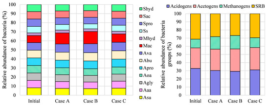
Figure 5.
Relative abundance of the bacterial community.
The optimal dosages of the Kemira BDP-840 additive were, in all cases, higher than at the initial state (experimental data). This additive promotes biogas production (Case A) as well as lower content in the produced biogas (Cases B and C). The optimized dosage of the enzymes provided by the SPF additive is, in all cases, higher than that actually added in the real biogas plant, Figure 6. The optimal dosage of the inorganic additive SPL was the lowest in Case B, followed by Cases C and A. Because of the lowest optimized values of the amount of SPL, it can be concluded that the conditions in the bioreactor in Case B are the most beneficial for the AD process; note that higher concentrations of inorganic additives can inhibit the AD process [14].
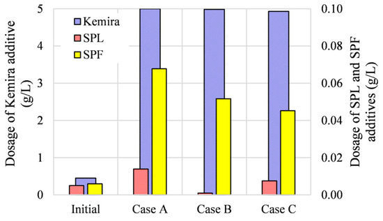
Figure 6.
Initial and optimized dosages of Kemira BDP-840, SPL, and SPF additives.
To estimate potential AD performance improvements, the quantity and quality of the produced biogas were analyzed in all cases by considering the impact of temperature, biological and inorganic additives, and their interactions. Some results with the most important findings are presented in the following.
In Cases A, B, and C, AD performances obtained by the optimized values of design variables were compared with those obtained by their initial values (initial state). The biogas flow rate for initial and optimal states is presented in Figure 7. The highest biogas flow rate reached Case A, where it increased by 30%. Meanwhile, in Cases B and C, the biogas production increased by about 14% and 1%, respectively. In Case A, the optimized temperature was increased to 60 . This high temperature is the main reason for increased biogas production, which is in accordance with the fact that thermophilic temperature can promote biogas production [4]. The high optimized dosage of the Kemira BDP-840 additive is another important reason for the highest biogas flow rate in Case A [42]. In Case B, where production was limited, the obtained optimal value of temperature was around 45 . In Case C, where the objective was to increase biogas production and reduce the bioreactor heating energy, the obtained optimal temperature was about 25 ; consequently, the biogas production rate could not increase essentially with respect to the initial state. Anyhow, by optimizing the dosage of biological and inorganic additives, it was possible to preserve the initial biogas production rate while ensuring a substantial decrease in temperature (lower heating cost). The relative biogas production rate (the production rate with respect to bioreactor volume) was in Case C, while the highest value of was obtained in Case A.

Figure 7.
Initial and optimized biogas flow rates.
The flow rate and content in biogas for initial and optimal states are presented in Figure 8. The highest production rate and content in biogas were reached in Case C. With respect to the initial state, the production rate was higher by 9%, 11%, and 12.5% in Cases A, B, and C, respectively. Figure 8 shows that there was no significant difference in flow rates among all three cases, but the content of in the produced biogas increased from Case A through Case B to Case C. The obtained results are in agreement with those presented by Cao et al. [43], who demonstrated that the highest content of could be reached at mesophilic temperature conditions. The best relative production rate of was reached in Case C.

Figure 8.
Initial and optimized flow rates.
The flow rate and content in biogas for initial and optimal states are presented in Figure 9. The smallest production was reached in Case C, where the relative production rate was lower by about 29% with respect to the initial state. With respect to the initial state, the relative production rate increased by about 11% in Case B and by about 87% in Case A. The highest relative production rate and the highest content in the produced biogas are obtained in Case A, where the optimized value of the temperature was the highest, and the optimized additives concentrations led to a low pH value. The obtained results are in agreement with Wang et al. [44], who reported that a thermophilic condition and low pH value lead to a higher hydrogen production rate.
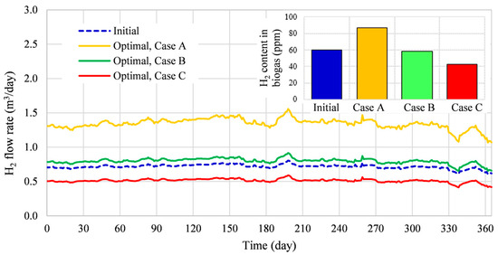
Figure 9.
Initial and optimized flow rates.
The flow rate and content in biogas at initial and optimal states are presented in Figure 10. The smallest production was reached in Case C. With respect to the initial state, the relative production rate was higher by about 114% in Case A and by about 22% in Case B. Only in Case C was the obtained relative production rate lower by about 20% when compared to the initial state. The lowest content in the produced biogas in Case C is the consequence of the interactions of low temperature and appropriate amounts of biological and inorganic additives, which influenced the value favorably.

Figure 10.
Initial and optimized flow rates.
The flow rate and the content in biogas for initial and optimal states are presented in Figure 11. The smallest production was reached in Case C. The relative production rate increased by about 270% in Case A and by about 43% in Case B with respect to the initial state; only Case C delivered the relative production rate of which was about 80% lower than at the initial state.

Figure 11.
Initial and optimized flow rates.
A comparison of the simulated value during the AD process at initial and optimal states in Cases A, B, C is presented in Figure 12. The average pH value during the 365 days of the AD process was 7.7 for the initial design; this value is close to the experimental one. The optimized average values were 7.5 in Case A, 7.6 in Case B, and 7.7 in Case C.

Figure 12.
Initial and optimized values.
The variations in the production of biogas and its compounds at optimal states (Cases A, B, and C) with respect to the initial state are presented in Figure 13. It can be seen that the increased biogas production in Case A is a consequence of the increase in all biogas compounds: , , , , , and vapour. The main part of the produced biogas is . Furthermore, in Case A, the content of vapour is the highest (more than 10%), while in Case C, it represents only 3%. This is expected since biogas typically contains 10% by volume of vapour at 43 , 5% by volume at 32 , and 1% by volume at 4.5 [45]. The constraint related to content in Cases B and C also influenced production, which increased with respect to production in Case A. By further adding constraints related to the contents of , , and in the produced biogas (Case C), and biogas production increased by 12.3% and 1.1%, while the production of , , and was reduced by 28.5%, 19.2%, and 80.9% with respect to the initial state.

Figure 13.
Variations in production of biogas and its compounds.
The variations in biogas compounds for optimized states (Cases A, B, and C) with respect to the initial state are presented in Figure 14. It is evident that in Case C, the content of desired increased by 11.1%, while the contents of undesired , , and reduced by 30%, 20%, and 81% when compared to the initial state.

Figure 14.
Variation in contents of biogas compounds.
The presented results show that temperature, biological additives (bacteria, enzymes), and inorganic additives (which impact the value), as well as their interaction, play an important role in the improvement of the AD process. Furthermore, the analysis of the obtained results shows that the optimization of the AD process in Case A delivers maximal biogas production, while the optimization in Case C maximizes the quality of the produced biogas.
4. Conclusions
This work investigated the suitability and efficiency of coupling a complex BioModel and an approximation-type gradient-based optimization method into a numerical optimization procedure during the AD process. Numerical experience has shown that the proposed approach provides a reliable and stable numerical procedure capable of optimizing the AD process quite efficiently. Moreover, no problems could be observed by engaging a gradient-based optimizer in combination with design derivatives and obtained by finite differences.
The best quality of biogas produced in reasonably large volumes at an acceptable cost can be reached by simultaneously maximizing biogas production and minimizing the heating energy needed. In this context, one must constrain the value, the maximal total initial concentrations of bacteria, minimal allowed content of and maximal allowed contents of , , and in the produced biogas. In such an optimization case, in this work, the content of in biogas increased by 11%, while the contents of , , and reduced by 30%, 20%, and 81%, respectively; in the optimized system, the bioreactor temperature was and the pH value was 7.7.
Since the proposed optimization procedure has shown itself to be numerically stable and efficient, future work should be focused in two directions. Firstly, the AD model should be further improved by considering more precise and various bacterial growth and inhibition models. Secondly, it would be beneficial to widen the AD process’s optimization possibilities by including parameters related to the feeding substrate and feeding strategy.
Author Contributions
Conceptualization, T.K. and B.K.; Methodology, T.K.; Software, T.K.; Validation, T.K.; Formal analysis, T.K.; Investigation, T.K.; Resources, T.K.; Data curation, T.K.; Writing—original draft preparation, T.K.; Writing—review and editing, T.K., M.K. and B.K.; Visualization, T.K.; Supervision, M.K. and B.K.; Project administration, T.K.; Funding acquisition, T.K., M.K. and B.K. All authors have read and agreed to the published version of the manuscript.
Funding
This research was funded by the Slovenian Research Agency, grant numbers P2-0414, P2-0032, P2-0196, and P2-0137 and the World Federation of Scientists, grant number SZF-T.Kegl-01/2023.
Data Availability Statement
The data presented in this study are available on request from the corresponding author. The data are not publicly available due to third party restrictions.
Acknowledgments
The authors are grateful for the financial support of the Slovenian Research Agency (core research funding No. P2-0414, P2-0032 P2-0196, and P2-0137). Tina Kegl also highly appreciates the fellowship granted by L’Oréal-UNESCO, Slovenia, under the program “For Women in Science 2022” and the fellowship granted by the World Federation of Scientists for year 2023/2024 (grant number SZF-T.Kegl-01/2023); special thanks go to Antonino Zichichi, WFS and to Edvard Kobal, Slovenian Science Foundation.
Conflicts of Interest
The authors declare no conflicts of interest.
References
- Kegl, T. Consideration of biological and inorganic additives in upgraded anaerobic digestion BioModel. Bioresour. Technol. 2022, 355, 127252. [Google Scholar] [CrossRef] [PubMed]
- Wu, D.; Peng, X.; Li, L.; Yang, P.; Peng, Y.; Liu, H.; Wang, X. Commercial biogas plants: Review on operational parameters and guide for performance optimization. Fuel 2021, 303, 121282. [Google Scholar] [CrossRef]
- Siddique, M.N.I.; Wahid, Z.A. Achievements and perspectives of anaerobic co-digestion: A review. J. Clean. Prod. 2018, 194, 359–371. [Google Scholar] [CrossRef]
- Neshat, S.A.; Mohammadi, M.; Najafpour, G.D.; Lahijani, P. Anaerobic co-digestion of animal manures and lignocellulosic residues as a potent approach for sustainable biogas production. Renew. Sustain. Energy Rev. 2017, 79, 308–322. [Google Scholar] [CrossRef]
- Van, D.P.; Fujiwara, T.; Tho, B.L.; Toan, P.P.S.; Minh, G.H. A review of anaerobic digestion systems for biodegradable waste: Configuration, operating parameters, and current trends. Environ. Eng. Res. 2020, 25, 1–17. [Google Scholar] [CrossRef]
- Kegl, T.; Kovač Kralj, A. An enhanced anaerobic digestion BioModel calibrated by parameters optimization based on measured biogas plant data. Fuel 2022, 312, 122984. [Google Scholar] [CrossRef]
- Obileke, K.H.; Nwokolo, N.; Makak, G.; Mukumba, P.; Onyeaka, H. Anaerobic digestion: Technology for biogas production as a source of renewable energy—A review. Energy Environ. 2021, 32, 191–225. [Google Scholar] [CrossRef]
- Hagos, K.; Zong, J.; Li, D.; Liu, C.; Lu, X. Anaerobic co-digestion process for biogas production: Progress, challenges and perspectives. Renew. Sustain. Energy Rev. 2017, 76, 1485–1496. [Google Scholar] [CrossRef]
- Kainthola, J.; Kalamdhad, A.S.; Goud, V.V. A review on enhanced biogas production from anaerobic digestion of lignocellulosic biomass by different enhancement techniques. Process Biochem. 2019, 84, 81–90. [Google Scholar] [CrossRef]
- Campos, E.; Flotats, X. Dynamic simulation of pH in anaerobic processes. Appl. Biochem. Biotechnol. 2003, 109, 63–76. [Google Scholar] [CrossRef]
- Paulo, L.L.; Stams, A.J.M.; Sousa, D.Z. Methanogens, sulphate and heavy metals: A complex system. Rev. Environ. Sci. Bio/Technol. 2015, 14, 537–553. [Google Scholar] [CrossRef]
- Abarghaz, Y.; el Ghali, K.M.; Mahi, M.; Werner, C.; Bendaou, N.; Fekhaoui, M.; Abdelaziz, B.H. Modelling of anaerobic digester biogas production: Case study of a pilot project in Morocco. J. Water Desalination 2013, 3, 381–391. [Google Scholar] [CrossRef]
- Mudhoo, A.; Kumar, S. Effects of heavy metals as stress factors on anaerobic digestion processes and biogas production from biomass. Int. J. Environ. Sci. Technol. 2013, 10, 1383–1398. [Google Scholar] [CrossRef]
- Guo, Q.; Majeed, S.; Xu, R.; Zhang, K.; Kakade, A.; Khan, A.; Hafeez, F.Y.; Mao, C.; Liu, P.; Li, X. Heavy metals interact with the microbial community and affect biogas production in anaerobic digestion: A review. J. Environ. Manag. 2019, 240, 266–272. [Google Scholar] [CrossRef] [PubMed]
- Lu, T.; Zhang, J.; Li, P.; Shen, P.; Wei, Y. Enhancement of methane production and antibiotic resistance genes reduction by ferrous chloride during anaerobic digestion of swine manure. Bioresour. Technol. 2020, 298, 122519. [Google Scholar] [CrossRef] [PubMed]
- Paritosh, K.; Yadav, M.; Chawade, A.; Sahoo, D.; Kesharwani, N.; Pareek, N.; Vivekanand, V. Additives as a support structure for specific biochemical activity boosts in anaerobic digestion: A review. Front. Energy Res. 2020, 8, 88. [Google Scholar] [CrossRef]
- Romero-Güiza, M.S.; Vila, J.; Mata-Alvarez, J.; Chimenos, J.M.; Astals, S. The role of additives on anaerobic digestion: A review. Renew. Sustain. Energy Rev. 2016, 58, 1486–1499. [Google Scholar] [CrossRef]
- Angelidaki, I.; Ellegaard, L.; Ahring, B.K. A mathematical model for dynamic simulation of anaerobic digestion of complex substrates: Focusing on ammonia inhibition. Biotechnol. Bioeng. 1993, 42, 159–166. [Google Scholar] [CrossRef]
- Angelidaki, I.; Ellegaard, L.; Ahring, B.K. A comprehensive model of anaerobic bioconversion of complex substrates to biogas. Biotechnol. Bioeng. 1999, 63, 363–372. [Google Scholar] [CrossRef]
- Flores-Alsina, X.; Solon, K.; Mbamba, C.K.; Tait, S.; Gernaey, K.V.; Jeppsson, U.; Batstone, D.J. Modelling phosphorus (P), sulfur (S) and iron (Fe) interactions for dynamic simulations of anaerobic digestion processes. Water Res. 2016, 95, 370–382. [Google Scholar] [CrossRef]
- Sun, H.; Yang, Z.; Zhao, Q.; Kurbonova, M.; Zhang, R.; Liu, G.; Wang, W. Modification and extension of anaerobic digestion model No. 1 (ADM1) for syngas biomethanation simulation: From lab-scale to pilot-scale. Chem. Eng. J. 2021, 403, 126177. [Google Scholar] [CrossRef]
- Maharaj, B.C.; Mattei, M.R.; Frunzo, L.; van Hullebusch, E.D.; Esposito, G. ADM1 based mathematical model of trace element precipitation/dissolution in anaerobic digestion processes. Bioresour. Technol. 2018, 267, 666–676. [Google Scholar] [CrossRef]
- Frunzo, L.; Fermoso, F.G.; Luongo, V.; Mattei, M.R.; Esposito, G. ADM1-based mechanistic model for the role of trace elements in anaerobic digestion processes. J. Environ. Manag. 2019, 241, 587–602. [Google Scholar] [CrossRef]
- Kovalovszki, A.; Alvarado-Morales, M.; Fotidis, I.A.; Angelidaki, I. A systematic methodology to extend the applicability of a bioconversion model for the simulation of various co-digestion scenarios. Bioresour. Technol. 2017, 235, 157–166. [Google Scholar] [CrossRef]
- Casallas-Ojeda, M.; Soto-Paz, J.; Alfonso-Morales, W.; Oviedo-Ocaña, E.R.; Komilis, D. Optimization of operational parameters during anaerobic co-digestion of food and garden waste. Environ. Process. 2021, 8, 769–791. [Google Scholar] [CrossRef]
- Huang, M.; Han, W.; Wan, J.; Ma, Y.; Chen, X. Multi-objective optimization for design and operation of anaerobic digestion using GA-ANN and NSGA-II. J. Chem. Technol. Biotechnol. 2016, 91, 226–233. [Google Scholar] [CrossRef]
- Beltramo, T.; Hitzmann, B. Evaluation of the linear and non-linear prediction models optimized with metaheuristics: Application to anaerobic digestion processes. Eng. Agric. Environ. Food 2019, 12, 397–403. [Google Scholar] [CrossRef]
- Elagroudy, S.; Radwan, A.G.; Banadda, N.; Mostafa, N.G.; Owusu, P.A.; Janajreh, I. Mathematical models comparison of biogas production from anaerobic digestion of microwave pretreated mixed sludge. Renew. Energy 2020, 155, 1009–1020. [Google Scholar] [CrossRef]
- Kegl, T.; Kovač Kralj, A. Multi-objective optimization of anaerobic digestion process using gradient-based algorithm. Energy Convers. Manag. 2020, 226, 113560. [Google Scholar] [CrossRef]
- SIST EN 15934:2012; Sludge, Treated Biowaste, Soil and Waste—Calculation of Dry Matter Fraction after Determination of Dry Residue or Water Content. Slovenian Institute for Standardization: Ljubljana, Slovenia, 2012.
- SIST EN 15935:2012; Sludge, Treated Biowaste, Soil and Waste—Determination of Loss on Ignition. Slovenian Institute for Standardization: Ljubljana, Slovenia, 2021.
- ASTM E1758-01R20; Standard Test Method for Determination of Carbohydrates in Biomass by High Performance Liquid Chromatography. ASTM International: West Conshohocken, PA, USA, 2020.
- SIST ISO 937-1978; Meat and Meat Products—Determination of Nitrogen Content (Reference Method). Slovenian Institute for Standardization: Ljubljana, Slovenia, 1978.
- SIST ISO 1443-1973; Meat and Meat Products—Determination of Total Fat Content. Slovenian Institute for Standardization: Ljubljana, Slovenia, 1973.
- ASTM D4373-02; Standard Test Method for Rapid Determination of Carbonate Content of Soils. ASTM International: West Conshohocken, PA, USA, 2007.
- SIST ISO 5664:1996; Water Quality, Determination of Ammonium. Slovenian Institute for Standardization: Ljubljana, Slovenia, 1996.
- SIST ISO 9280:1990; Water Quality, Determination of Sulfate. Slovenian Institute for Standardization: Ljubljana, Slovenia, 1990.
- SIST EN 16170:2016; Sludge, Treated Biowaste and Soil—Determination of Elements Using Inductively Coupled Plasma Optical Emission Spectrometry (ICP-OES). Slovenian Institute for Standardization: Ljubljana, Slovenia, 2016.
- SIST EN 26777:1996; Water Quality—Determination of Nitrite. Slovenian Institute for Standardization: Ljubljana, Slovenia, 1996.
- Kegl, M.; Butinar, B.J.; Kegl, B. An efficient gradient-based optimization algorithm for mechanical systems. Commun. Numer. Methods Eng. 2002, 18, 363–371. [Google Scholar] [CrossRef]
- Singh, A.; Moestedt, J.; Berg, A.; Schnürer, A. Microbiological surveillance of biogas plants: Targeting acetogenic community. Front. Microbiol. 2021, 12, 700256. [Google Scholar] [CrossRef]
- Zhang, H.; Tian, Y.; Wang, L.; Mi, X.; Chai, Y. Effect of ferrous chloride on biogas production and enzymatic activities during anaerobic fermentation of cow dung and Phragmites straw. Biodegradation 2016, 27, 69–82. [Google Scholar] [CrossRef] [PubMed]
- Cao, L.; Keener, H.; Huang, Z.; Liu, Y.; Ruan, R.; Xu, F. Effect of temperature and inoculation ratio on methane production and nutrient solubility of swine manure anaerobic digestion. Bioresour. Technol. 2020, 299, 122552. [Google Scholar] [CrossRef] [PubMed]
- Wang, Y.; Xi, B.; Li, M.; Jia, X.; Wang, X.; Xu, P.; Zhao, Y. Hydrogen production performance from food waste using piggery anaerobic digested residues inoculum in long-term systems. Int. J. Hydrogen Energy 2020, 45, 33208–33217. [Google Scholar] [CrossRef]
- al Mamun, M.R.; Torii, S. Enhancement of methane concentration by removing contaminants from biogas mixture using combined method absorption and adsorption. Int. J. Chem. Eng. 2017, 2017, 7906859. [Google Scholar] [CrossRef]
Disclaimer/Publisher’s Note: The statements, opinions and data contained in all publications are solely those of the individual author(s) and contributor(s) and not of MDPI and/or the editor(s). MDPI and/or the editor(s) disclaim responsibility for any injury to people or property resulting from any ideas, methods, instructions or products referred to in the content. |
© 2024 by the authors. Licensee MDPI, Basel, Switzerland. This article is an open access article distributed under the terms and conditions of the Creative Commons Attribution (CC BY) license (https://creativecommons.org/licenses/by/4.0/).