Article

A Diagnostic Curve for Online Fault Detection in AC Drives

by
Natalia Koteleva
1 and
Nikolai Korolev
2,*
1
Department of Automation of Technological Processes and Production, Empress Catherine II Saint Petersburg Mining University, 2, 21 Line of Vasilyevsky Island, 199106 St. Petersburg, Russia
2
Educational Research Center for Digital Technologies, Empress Catherine II Saint Petersburg Mining University, 2, 21 Line of Vasilyevsky Island, 199106 St. Petersburg, Russia
*
Author to whom correspondence should be addressed.
Energies 2024, 17(5), 1234; https://doi.org/10.3390/en17051234
Submission received: 31 January 2024 / Revised: 26 February 2024 / Accepted: 1 March 2024 / Published: 5 March 2024
(This article belongs to the Section F: Electrical Engineering)

Abstract

:
The AC drive is an important component and the most common element of any manufacturing process. A particularly serious task is the proper assessment of the AC drive’s technical condition, as its failure can cause problems for entire units and complexes of industrial enterprises. At present, there are several approaches either to determine electric drives’ condition or to find certain defects. Frequently, these methods require the installation of additional equipment that exceeds the price of the electric drive by several times. In this work, a simple approach is proposed. It includes the use of a diagnostic curve to assess the condition. This diagnostic curve is produced from the measurement results of the current sensors on the drive. Based on the Park vector modification, this is a simple and affordable way to obtain real-time information. The obtained curve can be used for the following purposes: directly for condition assessment by visual monitoring, as a sign for diagnostic systems built on artificial intelligence methods, for dynamic tuning of the drive control system. The article gives the algorithm for obtaining the diagnostic curve, showing its efficiency for model and field experiments. In model experiments, the faults in the rotor and stator of the drive were simulated; in field experiments, the state was analyzed by changing the load on the motor.

1. Introduction

The diagnostic methods of industrial facilities’ equipment are a high-priority task for numerous fields of industry (mining [1,2], oil and gas [3,4], metallurgical [5,6], etc.), in particular in terms of digitalization [7,8]. Continuous equipment performance and the prompt prediction of faults’ development allows us to formulate an effective vector of the enterprise activity and increase its efficiency [9,10]. Automated electric drive is a crucial element of any technological process. The assessment of its technical condition is an essential and high-priority task for the electric power industry, as well as for some related spheres, since the technical condition impacts the technological process [11,12]. The system of monitoring and the evaluation of the electric drive technical condition is not a unique scientific area. A lot of scientific papers are concerned with this matter [13,14]. Modern review articles [15,16] that cover the existing methods of AC drive diagnostics reveal several common trends in the development of diagnostics systems. These include the search for new means of measuring parameters [17,18], the search for algorithms for determining specific types of defects in electrical equipment [19,20], system approaches in solving diagnostic problems [21,22], and the use of artificial intelligence in diagnostic problems [23,24]. As we can conclude from the observed scientific papers, the given ways and means of diagnostics require additional investments in sensors, specialized devices and equipment, highly competent employees, system architecture, and others. Often these expenses are many times higher than the cost of the electric drive. In addition, it is more expedient to replace the motor with a new one [25,26]. In this regard, the development of a simple method of diagnostics that does not require, for example, large investments in the system or increasing the competence of the service personnel is clearly an important task. Currently, there are a few well-known studies that propose such diagnostic methods. In the article [27], the ratio of the DC current to the main motor current is used as a diagnostic variable. The resulting transformation value is used to evaluate the efficiency of the electric motor. The paper [28] proposes a method of searching for six predetermined faults using data from two accelerometers attached to electric motors and measuring the vibration in two different directions. The study [29] uses the analysis of zero-sequence currents to detect faults in induction motors. It is proved that harmonics present in the spectrum of zero-sequence voltage component are found in the spectrum of zero-sequence current components. Therefore, their comparison allows us to receive a set of characteristic frequencies for certain types of faults. The approach for the early diagnosis of rolling bearing failures is presented in the article [30]. For that purpose, a three-axis detection system on the rotor is applied for wire-free vibration measurements, and transformations by a simple FFT Hilbert envelope are used.
There are diagnostic approaches using currents and voltages and other electrical parameters. The articles [31,32,33] describe widely used methods of spectral and signature analysis of consumed phase currents of an asynchronous motor. These methods are highly informative and have a wide range of diagnosed defects. But they are difficult to use because it is necessary to implement highly productive hardware solutions for processing and storing large arrays.
Taking into account the above approaches and works, the authors concluded that it is urgent and necessary to develop a simple method of diagnostics, which does not require the installation of expensive equipment and most importantly does not require the preliminary classification of defects or other transformations. The method is available for use on any type of AC driver and under any operating conditions.
Hence, the primary hypothesis of this work is that a curve, being a mathematical transformation of the Park vector hodograph acquired from the real-time data of current sensors, is possible to be applied as a diagnostic tool to assess the state of the electric drive.
The structure of the present study is the following. Section 2: A description of the Park vector is provided, including the procedure of data transformation and the algorithm for obtaining the diagnostic curve. Section 3: The model of the field and experiments were conducted as a proof of the main article hypothesis. Section 4: Conclusions and general results were obtained.

2. Materials and Methods

The mathematical basis of the diagnostic curve proposed in this paper is the transformation of the Park (Gorev) vector [34,35]. These calculations, which are valid for a real electric motor, are derived by the following Equations (1) and (2) [36,37].
i d = 2 3 × i A 1 6 × i B 1 6 × i C
i q = 1 2 × i B 1 2 × i C
where
  • id, iq—currents consumed by asynchronous motor (AM) in the 2-phase rotating coordinate system dq;
  • iA, iB, iC—currents consumed by asynchronous motor (AM) in the 3-phase rotating system ABC.
According to the Park transform, the generalized current vector in the plane describes a special trajectory—a hodograph [38]. In this study, the hodograph is the main plot for obtaining the diagnostic curve of the electric drive. Figure 1 shows a visual scheme of producing such a curve.
Based on this scheme, the motor current sensor data are transformed as follows to obtain the curve:
  • Data scaling is performed (it is reasonable to use the maximum acceptable current sensor measurement limits as scaling coefficients). This way, the diagnostic curve does not exceed the specified range in any case;
  • The number of points per period is identified;
  • Park’s hodograph is plotted (since the data are pre-scaled, the hodograph will always lie in the plane Re [−1;1] and Im [−1;1]);
  • The amount of segments is determined. The segments will define the sensitivity of the obtained curve to various changes in the electric motor;
  • Segments are numbered sequentially from left to right, from top to bottom;
  • For each point in a period peak, the segment is defined, and the points array is formed from the segment numbers;
  • The resulting array is then sorted from the minimum to the maximum;
  • The obtained data points are represented on the graph.
The process of obtaining the diagnostic curve is presented in Algorithm 1.
Algorithm 1. Diagnostic curve
INPUT
1Get Ia,Ib,Ic from current sensor
2Set Kcur scaling coefficient
3Set Npoint number of points in period
4Set Nsegm number of segments
MAIN PROGRAM
5(IaSc,IbSc,IcSc) Scale current sensor values (using Kcur)
6(ParkRes) Get Park vector (using IaSc,IbSc,IcSc, Npoint)
7(SegmMtrx) Get Segment Matrix (using Nsegm)
8(PSegm) For each Npoint in ParkRes find segment number (using SegmMtrx)
9(SortPSegm) Sorting PSegm
OUTPUT
10Plotting the diagnostic curve (SortPSegm)

3. Experiments and Results

Both modeling and field experiments were conducted to prove the effectiveness of the offered method. Matlab Simulink v.2020b software was used for model experiments, a laboratory set with an electric drive—for full-scale experiments. The motor load of 20 and 40% of the rated values represents the varying parameters. Each experiment and its results are further described in the relevant sections.

3.1. Model Experiments

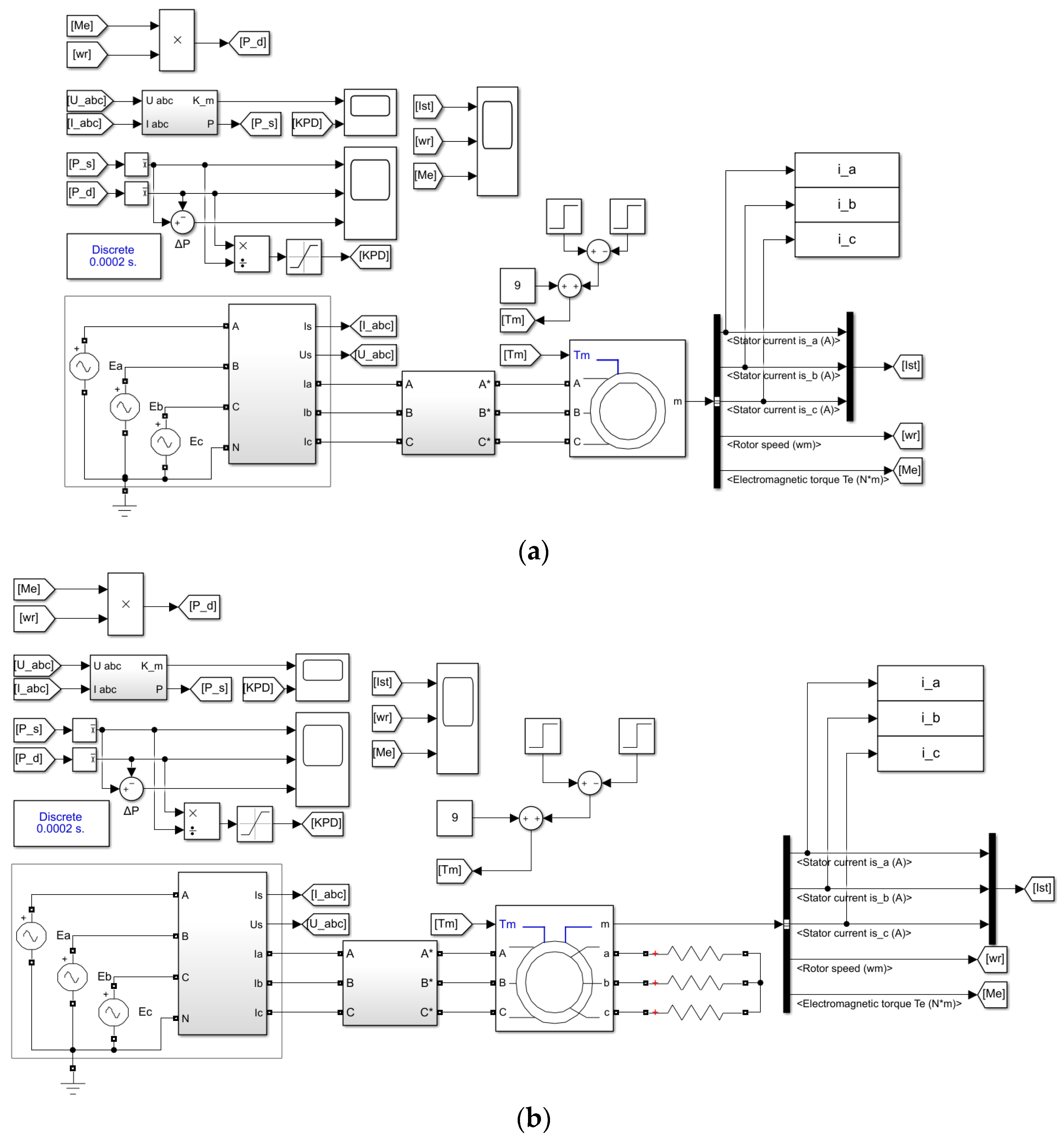
For the modeling experiments, a standard model was built in Matlab Simulink software. The visual form is presented in Figure 2. Figure 2a illustrates the sample model, closely simulating interturn and interphase faults due to phase short-circuits and changes in the equivalent resistances and parameters of the induction motor substitution diagram. In Figure 2b, the model can be seen. It is simulating the rotor bars’ breakage. In the simulation, the equivalent rotor resistances and parameters of the induction motor substitution scheme are changed.
The simulation was performed with the real parameters of the asynchronous motor indicated in Table 1 and Table 2 and corresponds to the laboratory set using in the experimental part. The direct start of the electric motor from the network with a voltage of 380 V and 50 Hz was implemented.
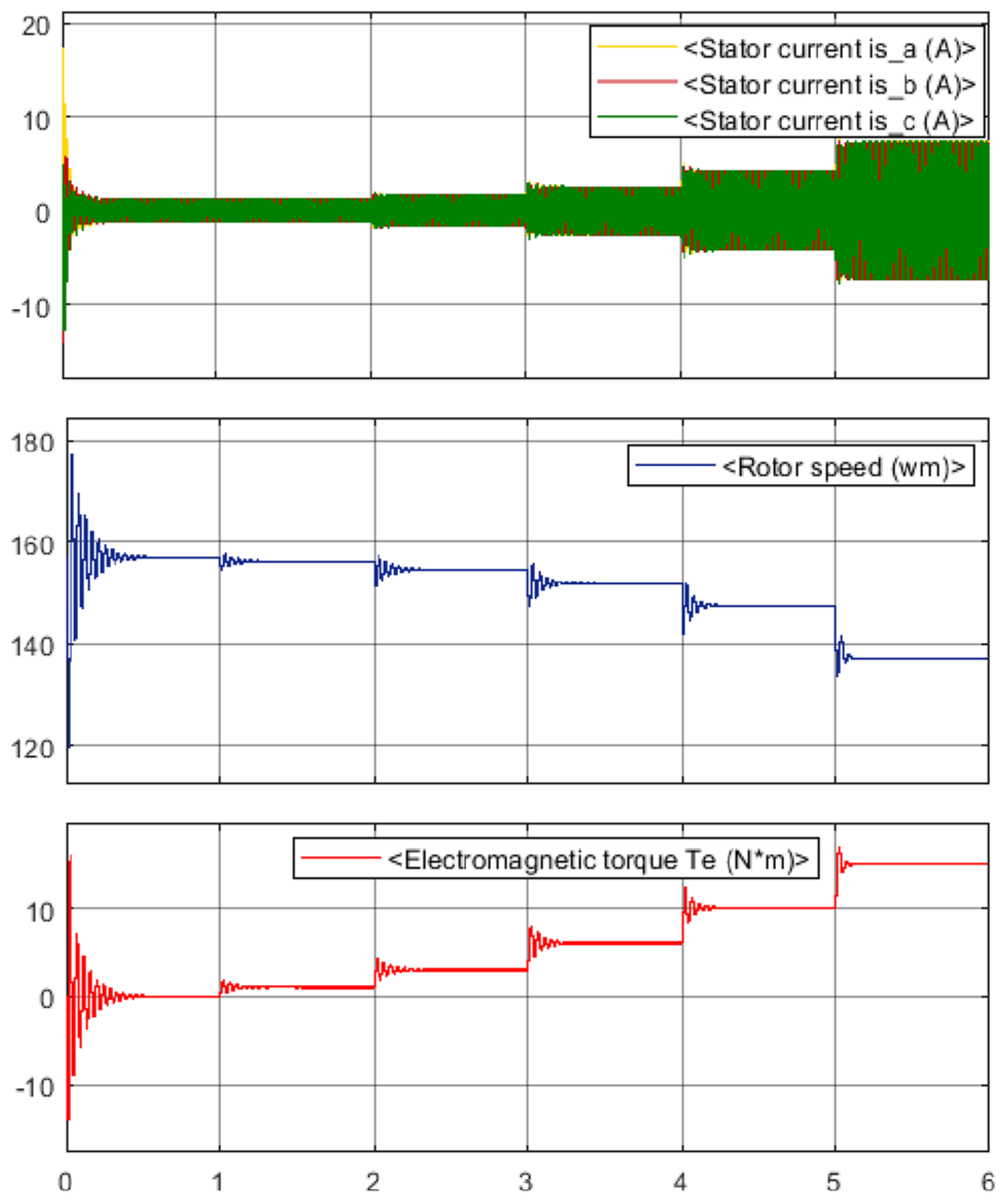
At the first stage, simulation was carried out using a step change in the nominal resistance torque. Simulation was started without load, and then the load was changed every 1 s by 10% of the nominal resistance torque (Figure 3).
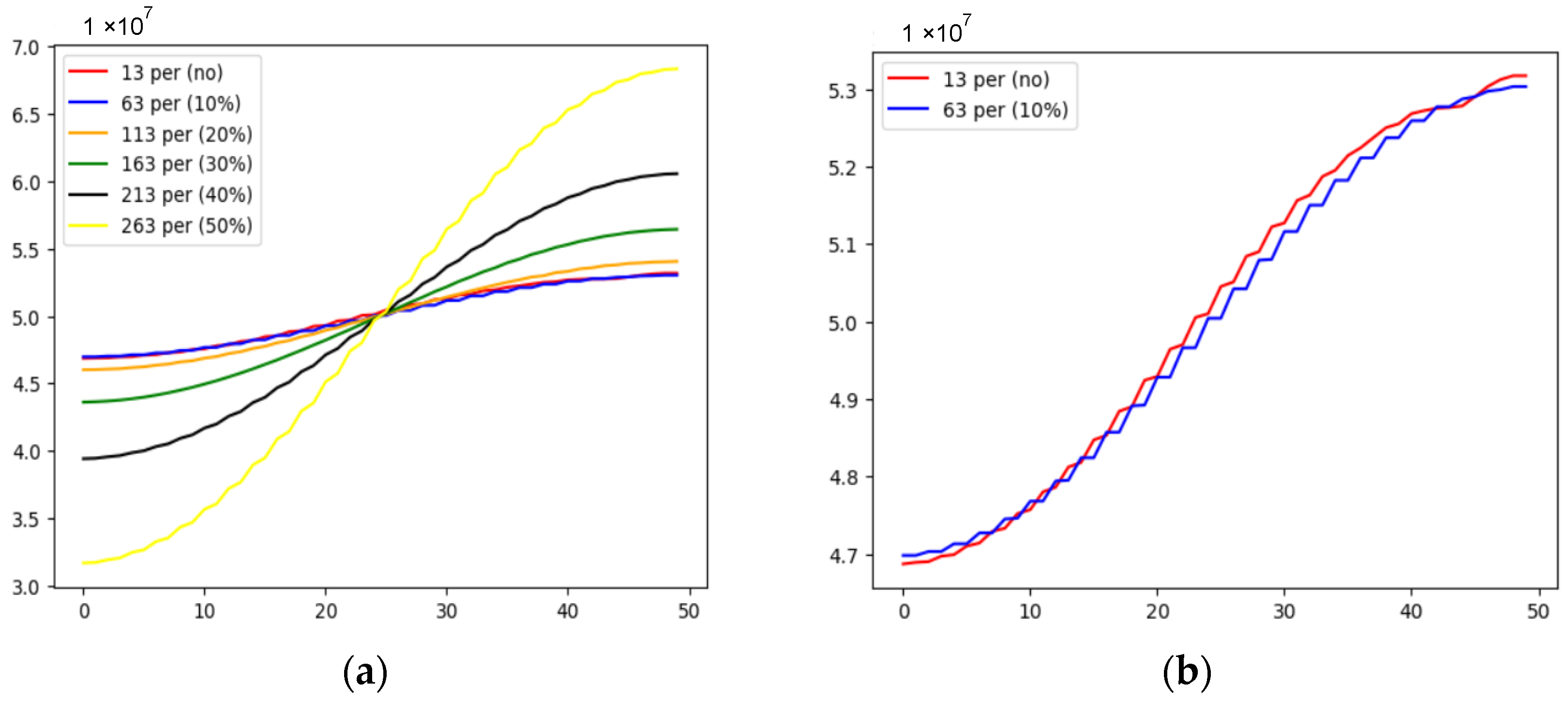
A step load change of 0–50% of the nominal resistance torque shows the character of the change in the diagnostic curve (Figure 4a). In this case, the deviation of the blue red line and the blue line is minimal, which characterizes normal operation without any deviations (Figure 4b).
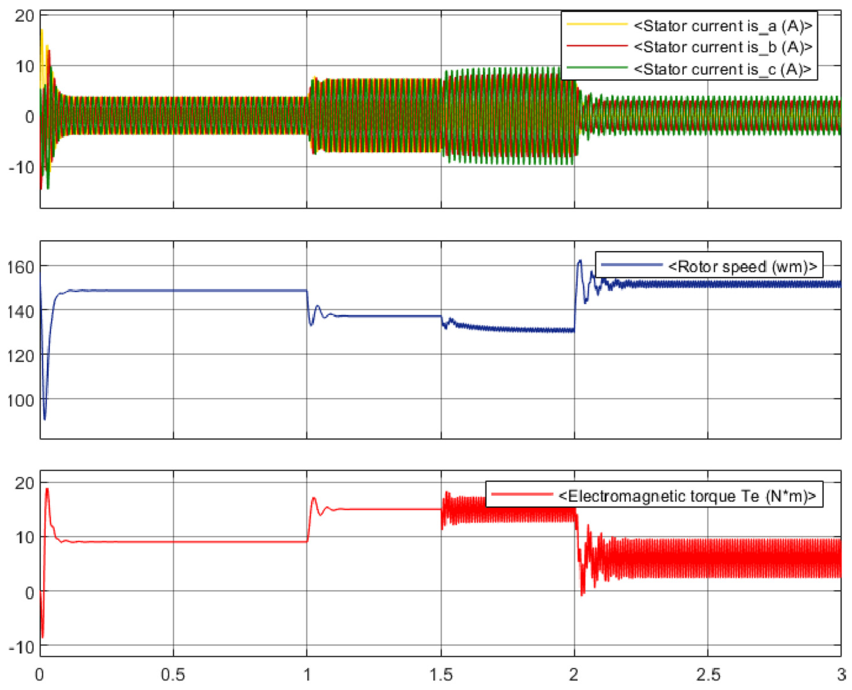
There are four drive states: starting at nominal resistance torque, running at nominal resistance torque, running at twice nominal resistance torque, and fault occurrence. Overall, three types of faults were simulated (stator short-circuit interturn phase A, stator short-circuit interphase phase AB, rotor bars’ breakage) in nine modifications (by resistance intensity: R_on = 1; R_on = 0.05; R_on = 0.01 Ohm (in the first and second cases), and Rc = 1, Rc = 3, Rc = 4 Ohm (in the third case)). Figure 3 shows the view of the simulated data for the stator short-circuit simulation case intercurrent phase A with resistance R_on = 1 Ohm, where R_on is the resistance value of the short circuit in the stator, and Rc is the equivalent resistance of the rotor when the rotor bars’ breakage.
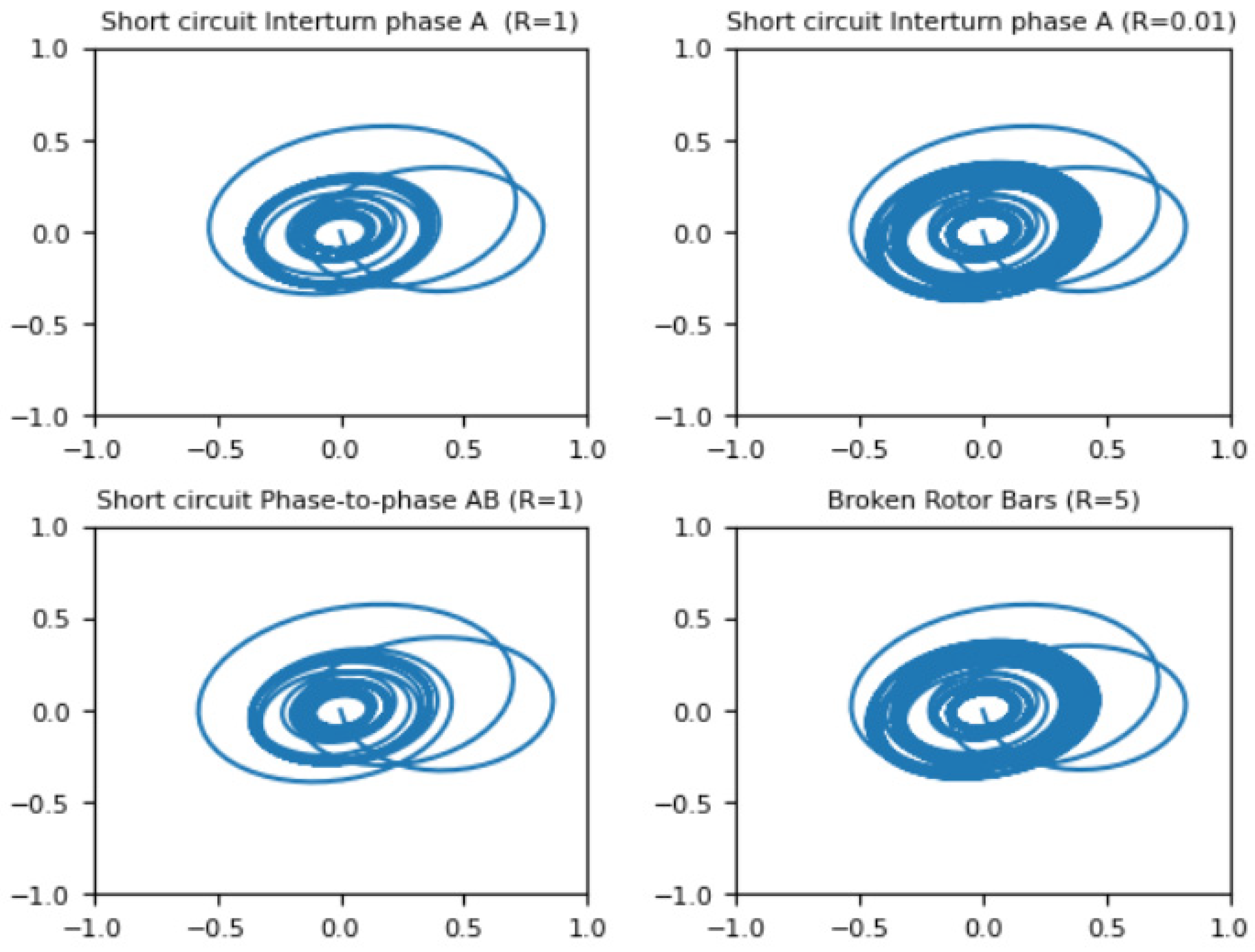
Figure 5 demonstrates the data of the next cases: motor start (T = 0–0.25 s start), motor operation at nominal resistance torque (T = 0.25–1 s, T = 2–3 s), motor operation at resistance torque increase two times nominal torque (T = 1–2 s), fault occurrence (T = 1.5 s). Figure 6 represents the Park vector hodograph for four cases described in the experiments (stator short-circuit interturn phase A with resistances R = 1 and R = 0.01 Ohm, stator short-circuit interphase AB with resistance R = 1 Ohm and rotor bars’ breakage with resistance R = 5 Ohm). The hodographs in Figure 6 reveal atypical variations (ellipse shape, thickening of the Park vector trajectory, misalignment). However, it is difficult to identify, decipher, and correlate the arising cases with the results of model experiments.
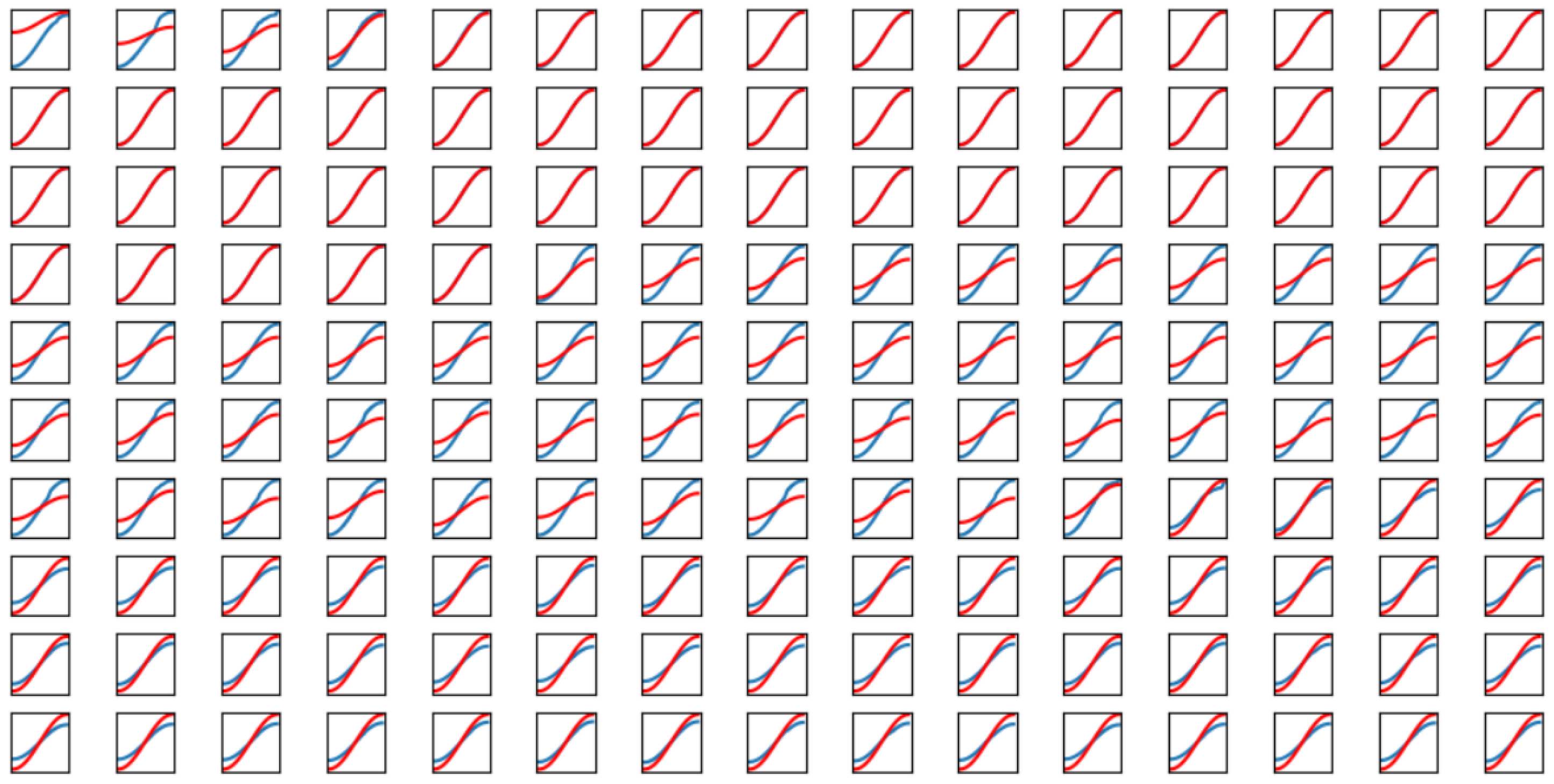
Figure 7 gives a general view of the diagnostic curves for the rotor bars’ breakage experiment with resistance R = 5 Ohm.
Figure 7 contains all 150 curves obtained during 3 s of simulation. In each case, two curves are shown, where the first is of the given period for the experiment (blue color) and the second is (red color) selected as a comparison and is the ideal. For all cases simulated, such a curve is obtained when the motor is operating at the nominal resistance torque. For this reason, we can notice only the red curve in the experiment periods from 4 to 49 (completely) and from 3.5 to 50 (partially), which corresponds to the time of 0.25–1 s. These are the times when the motor was in the operating mode at the nominal resistance torque. The curves of Figure 7 are also not very informative. Clearly, we can identify four different operating modes of the electric drive. If we look attentively, it is possible to recognize all five modes. However, this picture is informative for the whole experiment and the authors do not provide it to the user in this form for analysis. Still, the operating modes of the electric drive are more visible and, most critically, at what moments of time they were realized. This was complicated when using the hodograph.
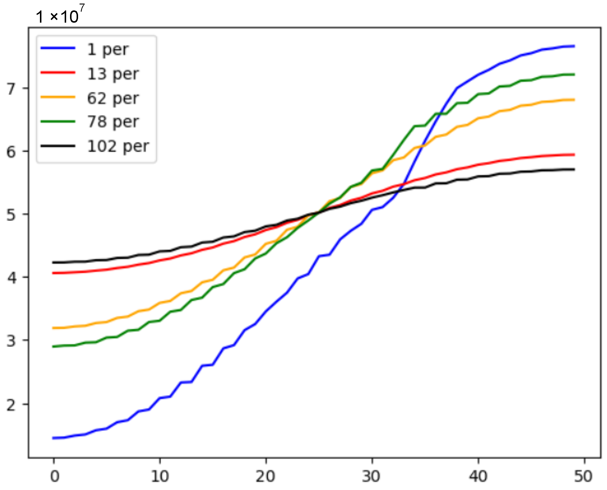
Figure 8 represents the diagnostic curves in random periods and corresponding to the five simulated cases.
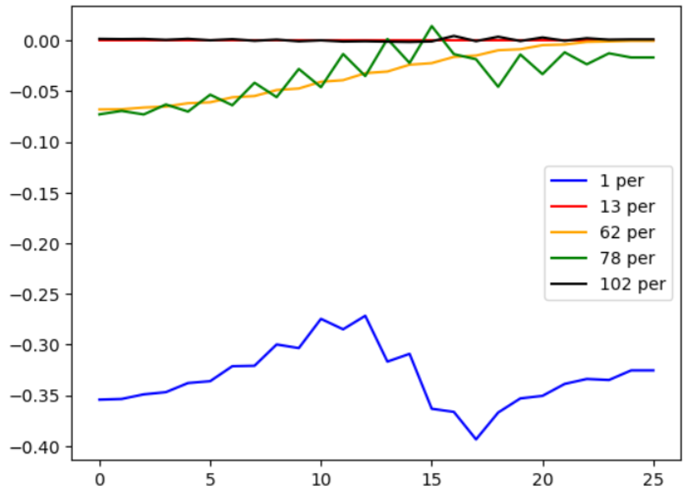
Figure 8 illustrates the differences in the diagnostic curves for the five modeled cases. The curves of the 13th, 62nd, and 102nd periods have a similar character, while the 1st and 78th periods are different. Indeed, in the first period the motor is started, and in the 78th period the fault is simulated. For better visualization, the user can also display a picture showing the symmetry of the curve relative to the center—in our case, the 25th period. Figure 9 shows the same case, but the curve has been transformed to demonstrate the symmetry.
According to Figure 9, the curves of Periods 13 and 102 are fully symmetric. After transformation, they are zero during all characteristic points. The curve of Period 62 is semi-symmetric, going to zero at the last points 24 and 25, and the curves of Periods 78 and 1 are completely asymmetric. Such characteristics were not easily observed from Figure 8.
Figure 10, Figure 11 and Figure 12 demonstrate the diagnostic curves for three experiments (stator short-circuit interturn phase A, stator short-circuit interphase AB, rotor bars’ breakage) at the moment of the faults’ occurrence (from Period 76 to 100), superimposed on each other with the resistances R = 1, R = 1, R = 1 Ohm (Figure 10), R = 0.05, R = 0.05, R = 3 Ohm (Figure 11), and R = 0.01, R = 0.01, R = 5 Ohm (Figure 12).
Figure 10, Figure 11 and Figure 12 indicate the evolution of the diagnostic curves as the influence of the defect increases. In the case of the lowest effect, there is also a difference, and thus it can be used for comparison with the defect or fault that is occurring. The curve state change successfully demonstrates both the degree of fault and the type of defect. In the model experiments, the number of segments to convert the hodograph into a diagnostic curve was chosen as 10,000. In all experiments, it is reasonable to increase the visibility by increasing the number of segments.

3.2. Full-Scale Experiments

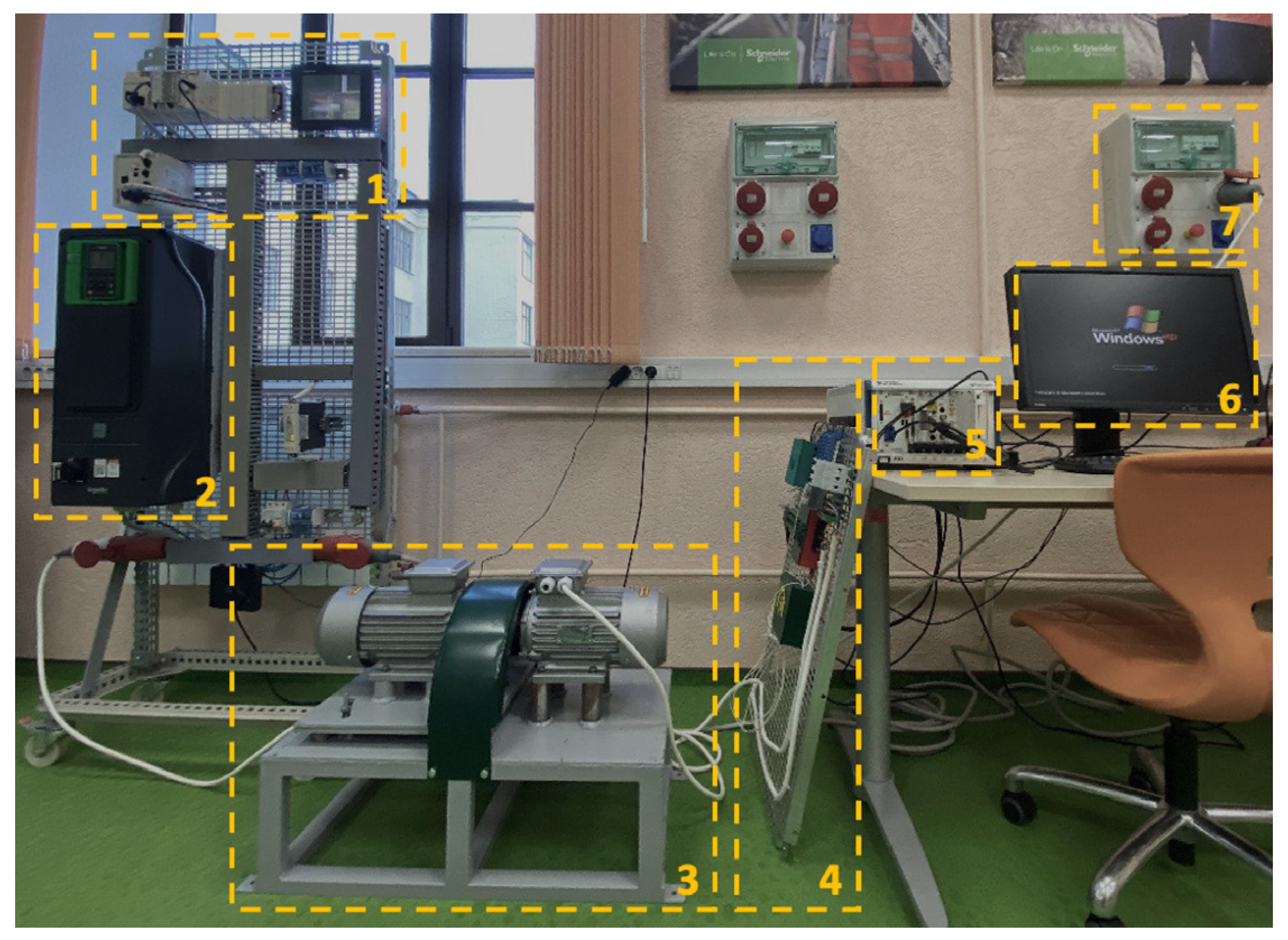
A laboratory set with an electric drive connected to the AC line was used to carry out full-scale experiments. Figure 13 shows the external view of the set.
At the laboratory unit (Figure 13), the experiment consisted of starting tested induction motors (3) from a 380 V 50 Hz network and changing the technical condition, as well as the load using load induction motors (3). The torque rotation speed of the load induction motors (3) was adjusted in steps by the frequency converter (2). The registration of currents in real time through current and voltage sensors was based on the Hall effect (4) and a high-frequency analog-to-digital converter (5).
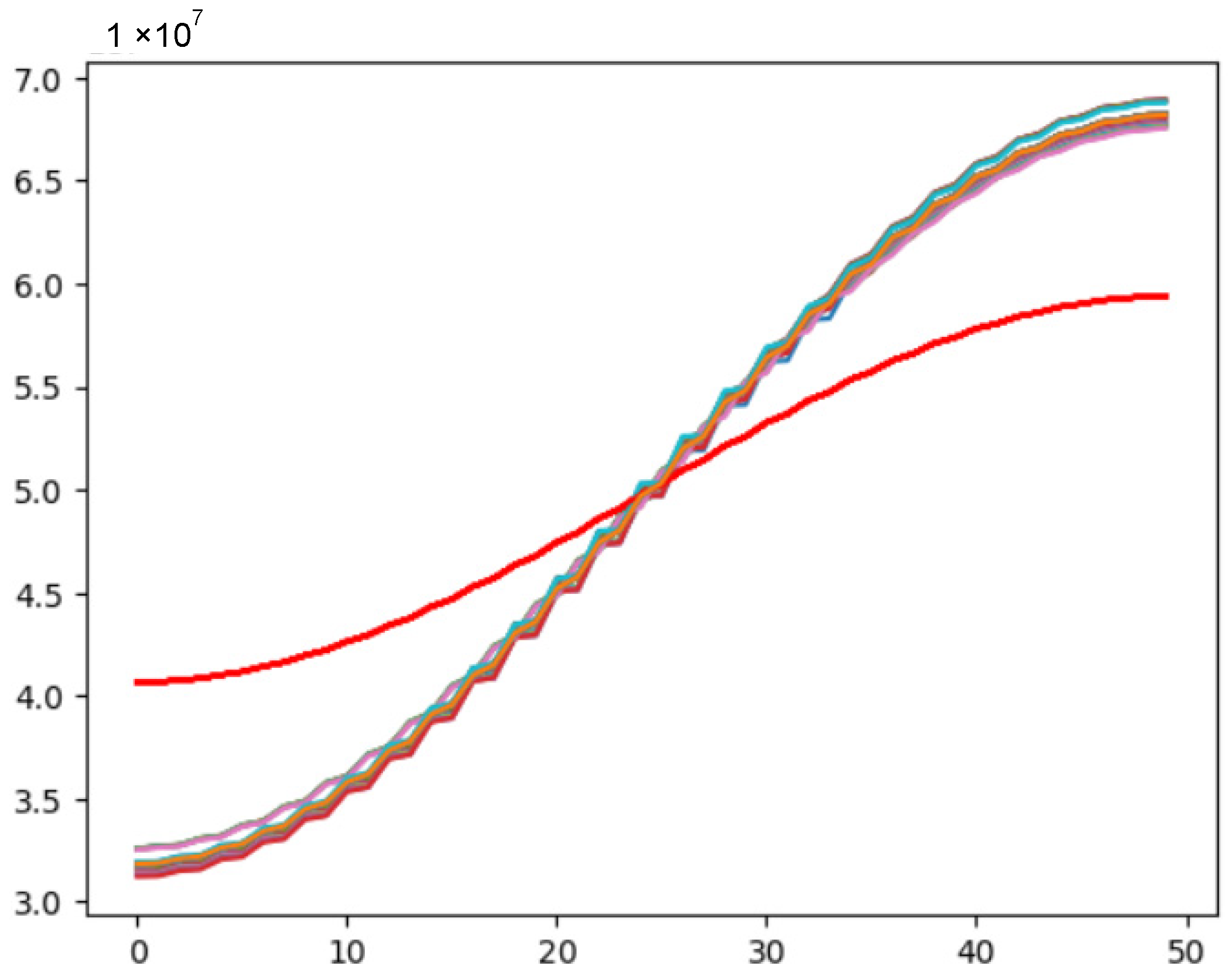
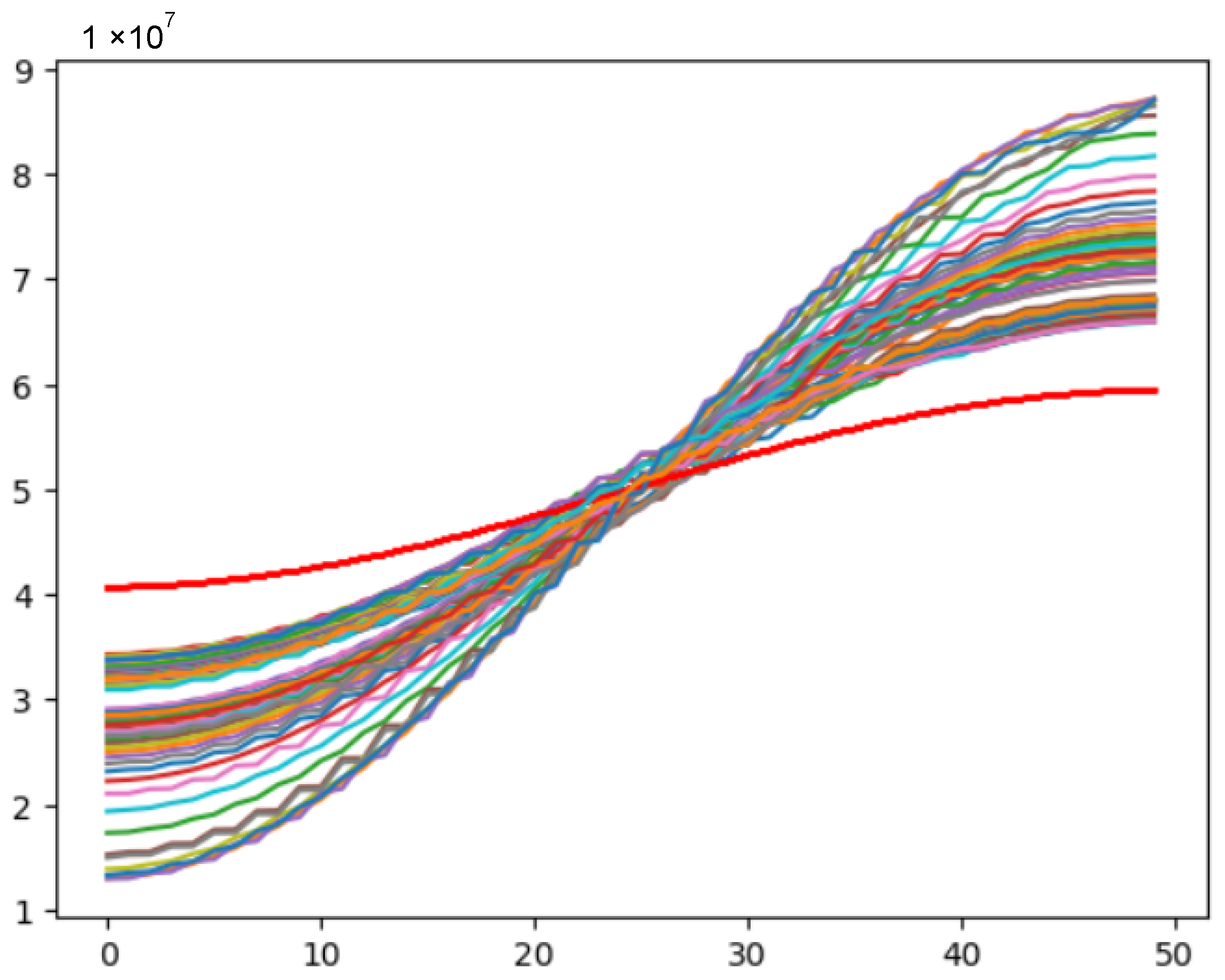
The laboratory setup presented in this work is not suitable for modeling the electric motor operation failure, so the simulation was reproduced partially. The motor loads of 20% and 40% of the nominal values were used as variables. As a reference diagnostic curve, the one obtained at the engine idle speed was chosen. The number of segments in full-scale experiments was equal to 1000. Figure 14, Figure 15 and Figure 16 show the experimental results.
Figure 14, Figure 15 and Figure 16 show the difference in the diagnostic curves modeling the three cases of load variation on the laboratory engine. An essential aspect is the fact that the diagnostic curve is obtained in real time. It means that the calculation resources do not exceed the period of polling the motor current sensors. This way, the diagnostic curve can be effectively implemented as a tool for the real-time assessment of the electric drive condition by specialists who are not highly competent and use only visual inspection methods. It is simple enough to evaluate the deviation from the curve set as a reference one for a given machine. In the present work, the idling curve of the motor without load was recorded in the software application as a reference.

4. Conclusions

The stated hypothesis has been proved in this paper. The curve, which is a mathematical transformation of the Park vector hodograph taken from the current sensor data in the real-time mode, can be used as a diagnostic tool to evaluate the electric drive condition. In this case, the diagnostic curve has a number of characteristics:
  • The diagnostic curve changes in real time and distorts the status of the drive for only the period of sensor polling;
  • The computing power is insufficient, so it can be displayed locally on a dashboard and provide a visual inspection tool for service engineers to monitor the drive condition;
  • The accuracy of the diagnostic curve is variable and depends on the number of segments dividing the Park vector space on which it is based;
  • The diagnostic curve always has an equal number of points, depending on the frequency of data collection and therefore on the current sensors used in the electric drive and its monitoring system;
  • Additionally, a graph evaluating the symmetry of the curve can be presented. In some cases, for full data symmetry it is acceptable to keep just half of the experimental data, which will significantly reduce the load on the system. However, this issue requires additional research;
  • The diagnostic curve could be useful as an independent means of diagnostics in visual inspection methods and as input data for more complex mathematical methods of diagnostics (e.g., neural networks independently or as an algorithm of feature generation), in electric motor control systems (algorithms and methods setting that allow to bring the existing diagnostic curve to the ideal one), etc.;
  • The diagnostic curve is convertible and, if needed, can be back-transformed to the Park vector hodograph and to sinus with insignificant distortions;
  • The diagnostic curve is a universal method of diagnostics and detection of the system deviations. It does not require any preliminary processing and labeling data and events, such as classification of defects, tuning to specific equipment modes, etc. The diagnostic curve can be applied to all types of AC motors under all operating conditions.

Author Contributions

Conceptualization, N.K. (Natalia Koteleva) and N.K. (Nikolai Korolev); methodology, N.K. (Natalia Koteleva); software, N.K. (Natalia Koteleva); validation, N.K. (Natalia Koteleva) and N.K. (Nikolai Korolev); formal analysis, N.K. (Natalia Koteleva) and N.K. (Nikolai Korolev); investigation, N.K. (Natalia Koteleva) and N.K. (Nikolai Korolev); resources, N.K. (Nikolai Korolev); data curation, N.K. (Nikolai Korolev); writing—original draft preparation, N.K. (Natalia Koteleva); writing—review and editing, N.K. (Nikolai Korolev); visualization, N.K. (Natalia Koteleva) and N.K. (Nikolai Korolev); supervision, N.K. (Nikolai Korolev); project administration, N.K. (Nikolai Korolev); funding acquisition, N.K. (Nikolai Korolev). All authors have read and agreed to the published version of the manuscript.

Funding

The research was performed with a grant from the Russian Science Foundation № 23-79-01292, https://rscf.ru/en/project/23-79-01292/, accessed on 29 February 2024.

Institutional Review Board Statement

Not applicable.

Informed Consent Statement

Not applicable.

Data Availability Statement

Data are contained within the article.

Conflicts of Interest

The authors declare no conflicts of interest.

References

  1. Dolzhikov, V.V.; Ryadinsky, D.E.; Yakovlev, A.A. Influence of deceleration intervals on the amplitudes of stress waves during the explosion of a system of borehole charges. MIAB Min. Inf. Anal. Bull. 2022, 6, 18–32. [Google Scholar] [CrossRef]
  2. Khokhlov, S.; Abiev, Z.; Makkoev, V. The Choice of Optical Flame Detectors for Automatic Explosion Containment Systems Based on the Results of Explosion Radiation Analysis of Methane- and Dust-Air Mixtures. Appl. Sci. 2022, 12, 1515. [Google Scholar] [CrossRef]
  3. Romashev, A.O.; Nikolaeva, N.V.; Gatiatullin, B.L. Adaptive Approach Formation Using Machine Vision Technology to Determine the Parameters of Enrichment Products Deposition. J. Min. Inst. 2022, 256, 677–685. [Google Scholar] [CrossRef]
  4. Yemelyanov, V.; Chernyi, S.; Yemelyanova, N.; Varadarajan, V. Application of neural networks to forecast changes in the technical condition of critical production facilities. Comput. Electr. Eng. 2021, 93, 107225. [Google Scholar] [CrossRef]
  5. Gizatullin, R.; Dvoynikov, M.; Romanova, N.; Nikitin, V. Drilling in Gas Hydrates: Managing Gas Appearance Risks. Energies 2023, 16, 2387. [Google Scholar] [CrossRef]
  6. Smirnov, N.I.; Drozdov, A.N.; Smirnov, N.N. Tribodynamic aspects of the resource of electric submersible vane pumps for oil production. J. Min. Inst. 2023, 264, 962–970. [Google Scholar]
  7. Litvinenko, V.S. Digital Economy as a Factor in the Technological Development of the Mineral Sector. Nat. Resour. Res. 2020, 29, 1521–15411. [Google Scholar] [CrossRef]
  8. Chen, Y.; Wang, Y.; Zhao, C. From riches to digitalization: The role of AMC in overcoming challenges of digital transformation in resource-rich regions. Technol. Forecast. Soc. Change 2024, 200, 123153. [Google Scholar] [CrossRef]
  9. Cherepovitsyn, A.E.; Tretyakov, N.A. Development of New System for Assessing the Applicability of Digital Projects in the Oil and Gas Sector. J. Min. Inst. 2023, 262, 628–642. [Google Scholar]
  10. Fomin, S.I.; Govorov, A.S. Validation of the chosen cutoff grade value in open pit mine design. MIAB Mining Inf. Anal. Bull. 2023, 12, 169–181. [Google Scholar] [CrossRef]
  11. Simakov, A.S.; Trifonova, M.E.; Gorlenkov, D.V. Virtual Analyzer of the Voltage and Current Spectrum of the Electric Arc in Electric Arc Furnaces. Russ. Metall. 2021, 2021, 713–719. [Google Scholar] [CrossRef]
  12. Khokhlov, S.; Safina, E.; Vasiliev, V. Risk-oriented approach implementation in departments ranking and teaching staff motivation. Int. J. Qual. Res. 2018, 12, 501–516. [Google Scholar] [CrossRef]
  13. Braut, S.; Sikanen, E.; Nerg, J.; Sopanen, J.; Božić, Ž. Fatigue life prediction of Electric Race About (ERA) traction motor rotor. Procedia Struct. Integr. 2021, 31, 45–50. [Google Scholar] [CrossRef]
  14. Accordini, D.; Cagno, E.; Trianni, A. Identification and characterization of decision-making factors over industrial energy efficiency measures in electric motor systems. Renew. Sustain. Energy Rev. 2021, 149, 111354. [Google Scholar] [CrossRef]
  15. Gultekin, M.A.; Bazzi, A. Review of Fault Detection and Diagnosis Techniques for AC Motor Drives. Energies 2023, 16, 5602. [Google Scholar] [CrossRef]
  16. Mian, Z.; Deng, X.; Dong, X.; Tian, Y.; Cao, T.; Chen, K.; Al Jaber, T. A literature review of fault diagnosis based on ensemble learning. Eng. Appl. Artif. Intell. 2024, 127, 107357. [Google Scholar] [CrossRef]
  17. Kohtz, S.; Zhao, J.; Renteria, A.; Lalwani, A.; Xu, Y.; Zhang, X. Kiruba Sivasubramaniam Haran, Debbie Senesky, Pingfeng Wang, Optimal sensor placement for permanent magnet synchronous motor condition monitoring using a digital twin-assisted fault diagnosis approach. Reliab. Eng. Syst. Saf. 2024, 242, 109714. [Google Scholar] [CrossRef]
  18. Yang, X.; Liu, M.; Song, H.; Zhu, S.; Wu, Y. Vibration resistance FBG temperature sensor fabrication and its application in the motor for hydraulic pump. Measurement 2022, 205, 112141. [Google Scholar] [CrossRef]
  19. D’Urso, D.; Chiacchio, F.; Borrometi, D.; Costa, A.; Compagno, L. Dynamic failure rate model of an electric motor comparing the Military Standard and Svenska Kullagerfabriken (SKF) methods. Procedia Comput. Sci. 2021, 180, 456–465. [Google Scholar] [CrossRef]
  20. He, H.; Han, M.; Liu, W.; Cao, J.; Shi, M.; Zhou, N. MPC-based longitudinal control strategy considering energy consumption for a dual-motor electric vehicle. Energy 2022, 253, 124004. [Google Scholar] [CrossRef]
  21. AlShorman, O.; Irfan, M.; Abdelrahman, R.B.; Masadeh, M.; Alshorman, A.; Sheikh, M.A.; Saad, N.; Rahman, S. Advancements in condition monitoring and fault diagnosis of rotating machinery: A comprehensive review of image-based intelligent techniques for induction motors. Eng. Appl. Artif. Intell. 2024, 130, 107724. [Google Scholar] [CrossRef]
  22. Aizpurua, J.I.; Knutsen, K.E.; Heimdal, M.; Vanem, E. Integrated machine learning and probabilistic degradation approach for vessel electric motor prognostics. Ocean Eng. 2023, 275, 114153. [Google Scholar] [CrossRef]
  23. Gao, Y.; Cheong, B.; Bozhko, S.; Wheeler, P.; Gerada, C.; Yang, T. Surrogate role of machine learning in motor-drive optimization for more-electric aircraft applications. Chin. J. Aeronaut. 2023, 36, 213–228. [Google Scholar] [CrossRef]
  24. Zhukovskiy, Y.; Buldysko, A.; Revin, I. Induction Motor Bearing Fault Diagnosis Based on Singular Value Decomposition of the Stator Current. Energies 2023, 16, 3303. [Google Scholar] [CrossRef]
  25. Gómez, J.R.; Sousa, V.; Eras, J.J.C.; Gutiérrez, A.S.; Viego, P.R.; Quispe, E.C.; de León, G. Assessment criteria of the feasibility of replacement standard efficiency electric motors with high-efficiency motors. Energy 2022, 239, 121877. [Google Scholar] [CrossRef]
  26. Errigo, A.; Choi, J.-K.; Kissock, K. Techno-economic-environmental impacts of industrial energy assessment: Sustainable industrial motor systems of small and medium-sized enterprises. Sustain. Energy Technol. Assess. 2022, 49, 101694. [Google Scholar] [CrossRef]
  27. Abramik, S.; Sleszynski, W.; Nieznanski, J.; Piquet, H. A diagnostic method for on-line fault detection and localization in VSI-fed AC drives. In Proceedings of the 10th European Conferenceon Power Electronicsand Applications, EPE’2003, Toulouse, France, 2–4 September 2003. [Google Scholar]
  28. Junior, R.F.R.; Areias, I.A.D.S.; Campos, M.M.; Teixeira, C.E.; da Silva, L.E.B.; Gomes, G.F. Fault detection and diagnosis in electric motors using 1d convolutional neural networks with multi-channel vibration signals. Measurement 2022, 190, 110759. [Google Scholar] [CrossRef]
  29. Duda, A.; Drozdowski, P. Induction Motor Fault Diagnosis Based on Zero-Sequence Current Analysis. Energies 2020, 13, 6528. [Google Scholar] [CrossRef]
  30. Wang, Z.; Shi, D.; Xu, Y.; Zhen, D.; Gu, F.; Andrew; Ball, D. Early rolling bearing fault diagnosis in induction motors based on on-rotor sensing vibrations. Measurement 2023, 222, 113614. [Google Scholar] [CrossRef]
  31. Yakhni, M.F.; Cauet, S.; Sakout, A.; Assoum, H.; Etien, E.; Rambault, L.; El-Gohary, M. Variable speed induction motors’ fault detection based on transient motor current signatures analysis: A review. Mech. Syst. Signal Process. 2023, 184, 109737. [Google Scholar] [CrossRef]
  32. Gu, F.; Shao, Y.; Hu, N.; Naid, A.; Ball, A.D. Electrical motor current signal analysis using a modified bispectrum for fault diagnosis of downstream mechanical equipment. Mech. Syst. Signal Process. 2011, 25, 360–372. [Google Scholar] [CrossRef]
  33. Suti, A.; Di Rito, G. Diagnosis of Power Switch Faults in Three-Phase Permanent Magnet Synchronous Motors via Current-Signature Technique. Actuators 2024, 13, 25. [Google Scholar] [CrossRef]
  34. Mendes, A.M.S.; Cardoso, A.J.M. Voltage source inverter fault diagnosis in variable speed AC drives, by the average current Park’s vector approach. In Proceedings of the IEEE International Electric Machines and Drives Conference, Seattle, WA, USA, 9–12 May 1999; Volume 6314016, pp. 704–706. [Google Scholar] [CrossRef]
  35. Muñoz-Aguilar, R.-S.; Rodríguez, P.; Dòria-Cerezo, A.; Candela, I.; Luna, A. A sensor-less sliding mode control scheme for a stand-alone wound rotor synchronous generator under unbalanced load conditions. Int. J. Electr. Power Energy Syst. 2014, 60, 275–282. [Google Scholar] [CrossRef]
  36. Cornell, E.P.; Lipo, T.A. Modeling and design of controlled current induction motor drive systems. IEEE Trans. Ind. Appl. 1977, 4, 321–330. [Google Scholar] [CrossRef]
  37. Thomson, W.T.; Fenger, M. Current signature analysis to detect induction motor faults. IEEE Ind. Appl. Mag. 2001, 7, 26–34. [Google Scholar] [CrossRef]
  38. Thomson, W.T.; Fenger, M.; Lloyd, B. Development of a tool to detect faults in induction motors via current signature analysis. In Proceedings of the Cement Industry Technical Conference, 2003, Conference Record, IEEE-IAS/PCA, Dallas, TX, USA, 4–9 May 2003; pp. 37–46. [Google Scholar] [CrossRef]
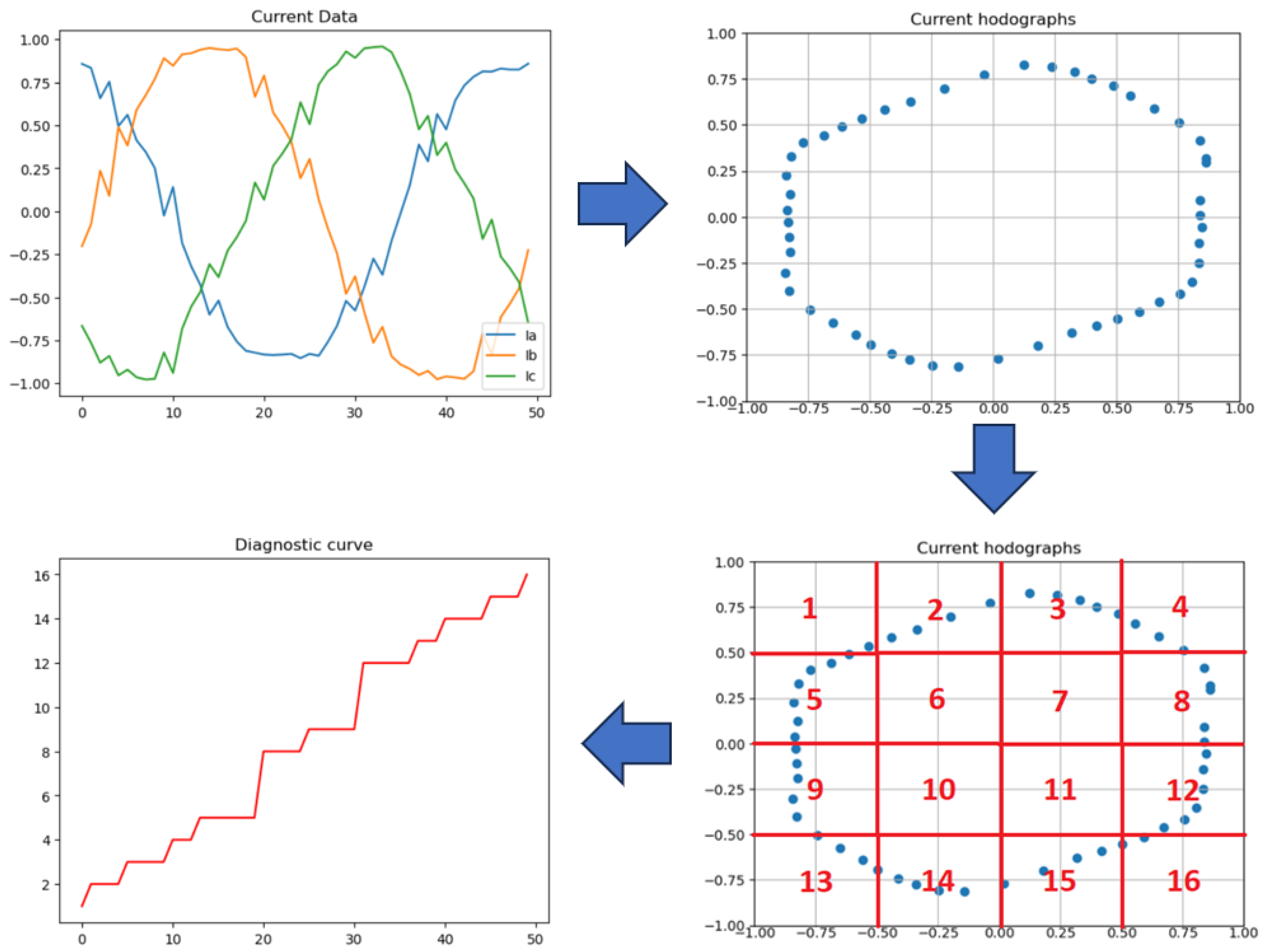
Figure 1. A visual scheme of producing a diagnostic curve.
Energies 17 01234 g001
Figure 2. Types of asynchronous motor: (a) with stator interturn short-circuit in phase A; (b) with rotor bars’ breakage.
Energies 17 01234 g002
Figure 3. Oscillogram of step load change.
Energies 17 01234 g003
Figure 4. Diagnostic curves for step load changes. (a) the diagnostic curve (13, 63, 113, 163, 213, 263 periods)…; (b) the diagnostic curve (13 and 63 periods)…
Energies 17 01234 g004
Figure 5. Oscillograms of the phase currents, rotor speed and electromagnetic moment for the stator short-circuit simulation case. Interturn phase A at equivalent short-circuit resistance R_on = 1 Ohm.
Energies 17 01234 g005
Figure 6. Hodograph of stator current Park vector for the 4 conditions of the induction motor.
Energies 17 01234 g006
Figure 7. Overall view (without scale) of diagnostic curves for the experiment of rotor bars’ breakage with resistance R = 5 Ohm (simulation time—3 s).
Energies 17 01234 g007
Figure 8. Diagnostic curves for the experiment of rotor bars’ breakage with resistance R = 5 Ohm, obtained in the 1st, 13th, 62nd, 78th, and 102nd periods of the experiment.
Energies 17 01234 g008
Figure 9. Diagnostic curves for the experiment of rotor bars’ breakage with resistance R = 5, obtained in the 1st, 13th, 62nd, 78th, and 102nd periods showing the symmetry property.
Energies 17 01234 g009
Figure 10. Diagnostic curves for these three experiments (stator interturn phase A, stator interphase AB, rotor bar breakage) at the moment of the faults’ occurrence (from Period 76 to 100), overlaid on each other with the resistances R = 1, R = 1, R = 1 Ohm.
Energies 17 01234 g010
Figure 11. Diagnostic curves for these three experiments (stator interturn phase A, stator interturn phase AB, rotor bar breakage) at the moment of the faults’ occurrence (from Period 76 to 100), overlaid on each other with the resistances R = 0.05, R = 0.05, R = 3 Ohm.
Energies 17 01234 g011
Figure 12. Diagnostic curves for these three experiments (stator interturn phase A, stator interturn phase AB, rotor bar breakage) at the moment of the faults’ occurrence (from Period 76 to 100), overlaid on each other with the resistances R = 0.01, R = 0.01, R = 5 Ohm.
Energies 17 01234 g012
Figure 13. The laboratory set-up for conducting full-scale experiments: 1—controller (Modicon M340); 2—frequency converter (Altivar Process ATV950U22N4E); 3—load and tested induction motors; 4—measurement circuit of current sensors (LA 25-NP/SP44) and voltage sensors (LV 25-P/SP5); 5—data acquisition chassis (PXI-6052); 6—personal computer; 7—power input 380 V.
Energies 17 01234 g013
Figure 14. Diagnostic curve for the off-load operation. Curve selected as the reference curve.
Energies 17 01234 g014
Figure 15. Diagnostic curve for the electric drive motor condition in operation with a 20% load.
Energies 17 01234 g015
Figure 16. Diagnostic curve for the electric drive motor condition in operation with a 40% load.
Energies 17 01234 g016
Table 1. Nominal parameters of IM.
Power
P, W
Voltage Source
Un, B
Rotor Speed
n, rpm
Number of Pole Pairs
z
Moment of Inertia
J, kg*m2
ηcosφ,KmKpKi,
1500380139020.00340.90.792.32.36.2
cosφ—power factor; η—efficiency factor; Km—torque capacity; Kp—starting torque ratio; Ki—starting current ratio.
Table 2. Parameters of IM equivalent circuit.
Ls, HLr, HLm, HRs, OhmRr, Ohm
0.85350.86360.82364.8434.168
Ls—stator magnetization inductance; Lr—rotor magnetization inductance; Lm—mutual magnetization inductance; Rs—stator active resistance; Rr—rotor active resistance.
Disclaimer/Publisher’s Note: The statements, opinions and data contained in all publications are solely those of the individual author(s) and contributor(s) and not of MDPI and/or the editor(s). MDPI and/or the editor(s) disclaim responsibility for any injury to people or property resulting from any ideas, methods, instructions or products referred to in the content.