Solution of the Simultaneous Routing and Bandwidth Allocation Problem in Energy-Aware Networks Using Augmented Lagrangian-Based Algorithms and Decomposition

Abstract

We discuss several algorithms for solving a network optimization problem of simultaneous routing and bandwidth allocation in green networks in a decomposed way, based on the augmented Lagrangian. The problem is difficult due to the nonconvexity caused by binary routing variables. The chosen algorithms, which are several versions of the Multiplier Method, including the Alternating Direction Method of Multipliers (ADMM), have been implemented in Python and tested on several networks’ data. We derive theoretical formulations for the inequality constraints of the Bertsekas, Tatjewski and SALA methods, formulated originally for problems with equality constraints. We also introduce some modifications to the Bertsekas and Tatjewski methods, without which they do not work for an MINLP problem. The final comparison of the performance of these algorithms shows a significant advantage of the augmented Lagrangian algorithms, using decomposition for big problems. In our particular case of the simultaneous routing and bandwidth allocation problem, these algorithms seem to be the best choice.

1. Introduction

In the 2022 year, data transmission networks consumed 260–360 TWh or 1–1.5% of the global electricity use [1]. A strong growth in demand for data center and network services is expected to continue at least until the end of this decade [2], especially because of video streaming and gaming. On the other hand, a global energy crisis causes increase in prices of electricity and energy commodities and the threat of their shortages. All this makes it more important than ever to use the network infrastructure efficiently to guarantee the highest possible quality of service with the lowest possible energy consumption.

In the standard approach, network congestion control along with active queue management algorithms try to minimize an aggregated cost with respect to source rates, assuming that routing is given and constant over the time scale of interest. However, it seems that it would be more effective to treat transport and network layers together and minimize cross-layer costs on the time scale of routing changes, taking into account the energy component.

In paper [3], an approach to solve such a simultaneous routing and flow rate optimization problem in energy-aware computer networks has been presented. The formulation considered two criteria. The first criterion was the cost of a bad quality of service, and the second was the energy consumption. It was earlier shown [4] that such problems, where routing variables are binary, even in the simplified version without the energy component, are NP-hard, which means that for bigger networks it is impossible to obtain the optimal solution in a reasonable time frame. The ordinary Lagrangian relaxation cannot help us to obtain a good assessment of the solution and, as it is in most of the integer linear programming (ILP) and mixed-integer nonlinear programming (MINLP) problems [5,6], a duality gap can be observed [7] (that is a nonzero difference between the minimum of the original problem and the maximum of the dual function) and the violation of many constraints.

In the case of nonconvex problems, the most popular remedy to obtain strong duality, that is the zero gap, and to ensure that the constraints are met is to use augmented Lagrangian [8,9,10,11,12,13,14] and the multiplier or, in other words, shifted penalty function method, based on it [15,16,17]. Since we solve a network MINLP problem, the only formulations interesting to us are those which involve nonconvex constraints or discrete sets. As is stated in [13], continuous optimization over concave constraints can be used to represent the integrality condition. The simplest method of conversion of a discrete set $\tilde{X}$ to an equality constraint with a continuous function for any $x\in X\subseteq {\mathbb{R}}^n$, where $\tilde{X}\subseteq X$ and X is compact, is to use a distance function $d(x,\tilde{X})={min}_{z\in \tilde{X}}∥x-z∥,\forall x\in X$ and the constraint $d(x,\tilde{X})=0$ [13]. Other methods of continuous reformulations of mixed-integer optimization problems that may be effective in some problems are presented in [18].

Unfortunately, although MILP and MINLP optimization problems have been present from the very beginning in the most important works on the augmented Lagrangian approach [15] and they are very important in practical problems [19,20,21,22], most of the works dealing with nonconvex problems consider only nonconvexity of the objective functions [23,24]. There are relatively few proposals of methods and algorithms also considering nonconvexity of constraints [21,25,26,27,28,29] and even in a recent paper the following statement can be found: “Despite the recent development of distributed algorithms for nonconvex programs, highly complicated constraints still pose a significant challenge in theory and practice” [30]. The proposed algorithms are rather complicated, involve many levels and loops, corrections, linearizations, etc. [21,30,31,32].

In our paper, we try to solve the two-layer network optimization problem using especially adapted classical methods proposed in the literature for problems with nonconvex constraints, which have also some potential for parallelization. Because of that, very intensively developed in the recent years methods from the ADMM family (Alternative Directions Method of Multipliers), which as a Gauss–Seidel type are sequential as such, are treated on an equal footing with others. If necessary, for example, when an algorithm has been formulated for a different type of constraints than those in our problem, we adapt it.

The paper is organized as follows. We first present the studied network problem in Section 2, which is one of the presented in [7]. Next, in Section 3 and Section 4, we review, respectively, the basic augmented Lagrangian algorithms proposed for problems with nonconvex constraints and the methods of their decompositions suitable for parallel computing with some modifications proposed by us. Section 5 describes the transformations of our problem to use the algorithms presented in Section 4. The results of numerical tests on network problems will be shown in Section 6, and the conclusions follow in Section 7.

2. Network Optimization Problem of Simultaneous Routing and Bandwidth Allocation in Energy-Aware Networks

We can describe the problem of optimizing routing and flow rates simultaneously as identifying scalar flow rates $x_w$ and routes (single paths) $b_w$ that satisfy network constraints for given source–destination pairs $\left(S\right(w),D(w\left)\right)$, where w is a demand (flow) from the set W, that deliver the minimal total cost. Routes $b_w$ are vectors built of binary indicator variables $b_{wl}$, whether a link l from the set L is used by the connection w.

The problem can be formulated in the following way [7]:

$$\underset{x,b,y}{min}\sum _{w\in W}\left[f_w(x_w,b_w)=\gamma {\left({\overline{x}}_w-x_w\right)}^2+\delta \sum _{l\in L}{b}_{wl}\right]$$

(1)

subject to (s.t.)

$$\sum _{\{i\in N|(i,j)\in A\}}{y}_{w,e(i,j)}-\sum _{\{k\in N|(j,k)\in A\}}{y}_{w,e(j,k)}=\left\{\begin{array}{cc}-x_w\hfill & j=S\left(w\right)\hfill \\ x_w\hfill & j=D\left(w\right)\hfill \\ 0\hfill & \mathrm{otherwise}\hfill \end{array}\right.\forall w\in W,\forall j\in N$$

(2)

$$\begin{array}{cccc}\hfill & 0<{\underline{x}}_w\le x_w\le {\overline{x}}_w,\hfill & \hfill & \forall w\in W\hfill \end{array}$$

(3)

$$\begin{array}{cccc}\hfill & \sum _{w\in W}{y}_{wl}\le c_l,\hfill & \hfill & \forall l\in L\hfill \end{array}$$

(4)

$$\begin{array}{cccc}\hfill & y_{wl}\ge 0,\hfill & \hfill & \forall w\in W,\forall l\in L\hfill \end{array}$$

(5)

$$\begin{array}{cccc}\hfill & y_{wl}\le b_{wl}{\overline{x}}_w,\hfill & \hfill & \forall w\in W,\forall l\in L\hfill \end{array}$$

(6)

$$\begin{array}{cccc}\hfill & \sum _{\{j\in N|(i,j)\in A\}}{b}_{w,e(i,j)}\le 1,\hfill & \hfill & \forall w\in W,\forall i\in N\hfill \end{array}$$

(7)

$$\begin{array}{cccc}\hfill & b_{wl}\in \{0,1\},\hfill & \hfill & \forall w\in W,\forall l\in L\hfill \end{array}$$

(8)

where N is the set of all nodes and A is the set of all arcs of the network.

This is the third formulation from the paper [7], denoted there by $P_{alt}$. The objective Function (1) is quadratic and convex. The first component of the function $f_w(x_w,b_w)$ expresses a cost for not delivering the full possible bandwidth for a connection $w\in W$. The second component expresses the total cost of energy used in the network by the connection $w\in W$. Flow conservation law equations are formulated with auxiliary real variables $y_{wl}$ (the function $e(.,.)$ numbers arcs) and binary variables $b_{wl}$, the equality (2), and three inequalities (5)–(7). Constraints (7) force single path routing and constraints (6) keep the relation between auxiliary variables and binary variables.

3. Augmented Lagrangian Algorithms

We consider the constrained optimization problem of the form

$$\underset{x\in X}{min}f\left(x\right)$$

(9)

          s.t.

$$h\left(x\right)=0$$

(10)

where the function $f:{\mathbb{R}}^n\to \mathbb{R}$ is continuous and differentiable, $h:{\mathbb{R}}^n\to {\mathbb{R}}^m$ is linear, $m<n$ and the set $X\subseteq {\mathbb{R}}^n$ is compact. For simplicity, we do not consider inequality constraints, because they can be either transformed to equality constraints (10) with the help of (additional) slack variables or be a part of the definition of the set X.

In the 1950s to solve the minimization problem (9)–(10) in the convex case, the Lagrangian relaxation method was proposed [33,34,35], using Lagrangian function $L:{\mathbb{R}}^{n+m}\to \mathbb{R}$ defined as

$$L(x,\lambda )=f\left(x\right)+{\lambda }^{T}h\left(x\right),$$

(11)

where $\lambda \in {\mathbb{R}}^m$ is the Lagrange multipliers vector. This method used the associated dual functional q for (11) given as

$$q\left(\lambda \right)=\underset{x\in X}{min}L(x,\lambda )$$

(12)

According to the duality theory, the solution maximizes the dual function with respect to the Lagrange multipliers vector, that is, we should calculate

$$\underset{\lambda \in {\mathbb{R}}^m}{max}q\left(\lambda \right)$$

(13)

Usually, we iterate alternately on x and $\lambda$ in the following way:

$$x^{k+1}=\underset{x\in X}{min}L(x,{\lambda }^k)$$

(14)

$${\lambda }^{k+1}={\lambda }^k+{\rho }_{k}h\left(x^{k+1}\right)$$

(15)

where ${\rho }_k$ is a scalar stepsize coefficient.

The major drawback of the Lagrangian relaxation method is the requirement that the problem should possess a convex structure, which reduces its applicability. Applying it to nonconvex problems, including problems with discrete variables, can result in a duality gap, whereby the maximum of the dual function does not equal the minimum of the original problem.

Powell [36] and Hestenes [37] convexified the problem (9)–(10) by adding the squared norm of the equality constraints

$$L_{\rho }(x,\lambda )=f\left(x\right)+{\lambda }^{T}h\left(x\right)+\frac{\rho }{2}\left|\right|h\left(x\right)|{|}^2$$

(16)

where $\rho >0$ is a scalar, penalty parameter. This function is convex in the neighborhood of $(x^{*},{\lambda }^{*})$ when $\rho$ is taken sufficiently large and if at $(x^{*},{\lambda }^{*})$ the second order sufficient optimality condition

$$z^T{\nabla }_{xx}^{2}L(x^{*},{\lambda }^{*})z>0,\forall z\in {\mathbb{R}}^n,z\ne 0\mathrm{s}\mathrm{u}\mathrm{c}\mathrm{h} \mathrm{t}\mathrm{h}\mathrm{a}\mathrm{t}\nabla h{\left(x^{*}\right)}^{T}z=0$$

(17)

is satisfied.

The method of multipliers algorithm for solving problem (9)–(10), based on the augmented Lagrangian, consists of the following iterations:

$$x^{k+1}=\underset{x\in X}{min}{L}_{\rho }(x,{\lambda }^k)$$

(18)

$${\lambda }^{k+1}={\lambda }^k+{\rho }_{k}h\left(x^{k+1}\right)$$

(19)

When $X={\mathbb{R}}^n$, to reduce the steps of the (18)–(19) algorithm, a multiplier estimate function derived from the first order Karush–Kuhn–Tucker optimality condition [33] can be used [38,39]:

$$\lambda \left(x\right)=arg\underset{\lambda }{min}{∥{\nabla }_{x}L(x,\lambda )∥}^2=-{\left[\nabla h{\left(x\right)}^T\nabla h\left(x\right)\right]}^{-1}\nabla h{\left(x\right)}^T\nabla f\left(x\right),$$

(20)

This formula is particularly useful when it is possible to calculate analytically $\lambda \left(x\right)$, e.g., when functions $h\left(x\right)$ are linear. Then, having $\lambda \left(x\right)$, one can replace the two-level algorithm (18)–(19) with a single-level one:

$$x^{k+1}=\underset{x}{min}{L}_{\rho }(x,\lambda \left(x\right))$$

(21)

4. Separable Problems and Their Decomposition Algorithms

4.1. Classical Separable Problem Formulation

The problem (9)–(10) is said to be separable if it can be written as

$$\underset{x\in X}{min}\left[f\left(x\right)=\sum _{i=1}^N{f}_i\left(x_i\right)\right]$$

(22)

$$s.t.h\left(x\right)=\sum _{i=1}^N{h}_i\left(x_i\right)=0,$$

(23)

$$X=X_1\times X_2\times \dots X_N,X_i\subseteq {\mathbb{R}}^{n_i},i=1,\dots ,N$$

(24)

where $x_i\in {\mathbb{R}}^{n_i}$ are subvectors of decision variables, $x=(x_1,\dots ,x_N)\in {\mathbb{R}}^n$, $n={\sum }_{i=1}^N{n}_i$, $h_i:{\mathbb{R}}^{n_i}\to {\mathbb{R}}^m$ are given vector functions that describe constraints, and $f_i:{\mathbb{R}}^{n_i}\to \mathbb{R}$, $i=1,\dots ,N$. The set X is a Cartesian product of the sets $X_i$ in the corresponding subspaces.

The augmented Lagrangian for (22)–(24) can be written as

$$L_{\rho }(x,\lambda )=\sum _{i=1}^N{f}_i\left(x_i\right)+{\lambda }^T\sum _{i=1}^N{h}_i\left(x_i\right)+\frac{\rho }{2}{∥\sum _{i=1}^N{h}_i\left(x_i\right)∥}^2$$

(25)

The separable problem (22)–(24) yields a nonseparable Lagrange function due to the last-quadratic-penalty term, hence decomposition algorithms cannot be applied directly to the dual equivalent of the problem (22)–(24). To avoid the nonseparability, some tricks are necessary, which we describe in the following subsections. The most important conditions of the convergence of the presented algorithms to the optimal point $x^{*}$ for sufficiently big $\rho$ are that all functions from the problem statement are of class $C^2$ in a neighborhood of the optimal point $x^{*}$, gradients of all active constraints are linearly independent at $x^{*}$, and that the second order sufficient optimality condition (17) is satisfied (for the ordinary Lagrangian of the problem).

4.2. Bertsekas Decomposition Method

Bertsekas [25] proposed a convexification method that preserves the separability of a modified Lagrangian. It belongs to the proximal point algorithms family and may be interpreted as a multipliers method in disguise [40]. The penalty component expresses now not the square of the constraints function norm but the square of the distance between the x vector and a parameter vector s from its vicinity. In subsequent iterations, this vector approaches x, leading to convergence, while preserving separability. The resulting Lagrangian is

$$L_{\rho }(x,\lambda ,s)=f\left(x\right)+{\lambda }^{T}h\left(x\right)+\frac{\rho }{2}{∥s-x∥}^2$$

(26)

This function is separable and locally convex for $\rho$ from some interval provided that the above mentioned conditions are satisfied at point $x^{*}$ [25]. In a decomposed form, the augmented Lagrangian (26) can be written as

$$L_{\rho }(x,\lambda ,s)=\sum _{i=1}^N\left[f_i\left(x_i\right)+{\lambda }^T{h}_i\left(x_i\right)+\frac{\rho }{2}{∥s_i-x_i∥}^2\right]\triangleq \sum _{i=1}^N{L}_{{\rho }_i}(x_i,\lambda ,s_i)$$

(27)

where

$$L_{{\rho }_i}(x_i,\lambda ,s_i)=f_i\left(x_i\right)+{\lambda }^T{h}_i\left(x_i\right)+\frac{\rho }{2}{∥s_i-x_i∥}^2$$

(28)

The Bertsekas [25] approach was adapted by us to an MINLP problem. The most efficient proved to be a two-level version with additional scaling coefficient $\beta \ll 1$ in the formula for changing Lagrange multipliers. This algorithm may be described by the following steps:

$$\begin{array}{ccc}\hfill & x_i^{k+1}& =arg\underset{x_i\in X_i}{min}{L}_{{\rho }_i}\left(x_i,{\lambda }^k,s_i^k\right),i=1,\dots ,N\hfill \end{array}$$

(29)

$$\begin{array}{ccc}& s_i^{k+1}& =\xi s_i^k+(1-\xi )x_i^{k+1},i=1,\dots ,N\hfill \end{array}$$

(30)

$$\begin{array}{ccc}& {\lambda }^{k+1}& ={\lambda }^k+\beta \rho h\left(x^{k+1}\right)\hfill \end{array}$$

(31)

where $\xi \in [0,1)$ is a relaxation parameter.

4.3. Tanikawa–Mukai Decomposition Method

In the case when in the Bertsekas algorithm $X={\mathbb{R}}^n$, we may apply the approximation of the multipliers vector $\lambda \left(x\right)$ using the direct formula (20). Unfortunately, when $\lambda \left(x\right)$ substitutes $\lambda$ in (26), the resulting Lagrangian will no longer be separable, because of the term $\lambda {\left(x\right)}^{T}h\left(x\right)$, containing products of functions of different $x_i$ components, $i=1,\dots ,N$. Hence, separability will be preserved if $\lambda$ does not depend on x. To address this issue, Tanikawa and Mukai [26] replaced $\lambda \left(x\right)$ with an approximate $\lambda \left(s\right)$ and added a penalty term $\eta h{\left(s\right)}^{T}M\left(s\right)h\left(x\right)$ so as to ensure that the minimum point $\widehat{s}$ is closer than s to $x^{*}$. These improvements resulted in the formula

$$L_{\rho \eta }(x,s)=f\left(x\right)+\frac{\rho }{2}{∥x-s∥}^2+\left[\lambda {\left(s\right)}^T+\eta h{\left(s\right)}^{T}M\left(s\right)\right]h\left(x\right)$$

(32)

where $\eta >0$ is a scalar, and $M\left(s\right)$ is a symmetric, positive-definite matrix whose elements are of $C^1$ class. The Lagrangian problem (32) is locally strictly convex in x in the neighborhood of $x^{*}$ if $\rho$ is taken large enough and it has a unique local minimum point $s^{*}$ as a function of s.

In a decomposed form, (32) can be written as

$$L_{\rho \eta }(x,s)=\sum _{i=1}^N{L}_{{\rho \eta }_i}(x_i,s)$$

(33)

where

$$L_{{\rho \eta }_i}(x_i,s)=f_i\left(x_i\right)+\frac{\rho }{2}\left|\right|x_i-s_i|{|}^2+(\lambda {\left(s\right)}^T+\eta h{\left(s\right)}^{T}M\left(s\right))h_i\left(x_i\right)$$

(34)

The problem (22)–(24) for $X={\mathbb{R}}^n$ can now be solved by a two-level algorithm,

$$\begin{array}{ccc}\hfill & x_i^{k+1}& =arg\underset{x_i}{min}{L}_{{\rho \eta }_i}(x_i,s^k),i=1,\dots ,N\hfill \end{array}$$

(35)

$$\begin{array}{ccc}\hfill & s^{k+1}& ={\xi }_k{s}^k+(1-{\xi }_k)x^{k+1},{\xi }_k\in [0,1)\hfill \end{array}$$

(36)

Tatjewski and Engelmann [28] extended this approach to a more general case of the problem (22)–(24), involving local sets $X_i$, given by inequality constraints

$$X_i=\{x_i\in {\mathbb{R}}^{n_i}|g_i\left(x_i\right)\le 0\}$$

(37)

In this case, the Lagrange multipliers vector was calculated from the following formula:

$$\lambda (x,\mu )=-{\left[\nabla h{\left(x\right)}^T\nabla h\left(x\right)\right]}^{-1}\nabla h{\left(x\right)}^T\left[\nabla f\left(x\right)+\nabla g\left(x\right)\mu \right],$$

(38)

where $\mu$ is the multipliers vector for local inequality constraints

$$g_i\left(x_i\right)\le 0,i=1,\dots ,r$$

(39)

4.4. Tatjewski Decomposition Method

A different approach to handle the nonseparable term in the Function (25) with local sets $X_i$ given by (37), proposed by Tatjewski [27], consists in replacing the Function (25) by

$$L_{\rho }(x,\lambda ,s)=\sum _{i=1}^N{f}_i\left(x_i\right)+{\lambda }^T\sum _{i=1}^N{h}_i\left(x_i\right)+\frac{\rho }{2}\sum _{i=1}^N{∥\sum _{j=1,j\ne i}^N{h}_j\left(s_j\right)+h_i\left(x_i\right)∥}^2$$

(40)

where $s=(s_1,s_2,\dots ,s_N)\in R^n$ is an approximation point. The Function (40) is separable

$$L_{\rho }(x,\lambda ,s)=\sum _{i=1}^N{L}_{{\rho }_i}(x_i,\lambda ,s),$$

(41)

where

$$L_{{\rho }_i}(x_i,\lambda ,s)=f_i\left(x_i\right)+{\lambda }^T{h}_i\left(x_i\right)+\frac{\rho }{2}{∥\sum _{j=1,j\ne i}^N{h}_j\left(s_j\right)+h_i\left(x_i\right)∥}^2$$

(42)

The algorithm, which we adapted to an MINLP problem, has, as in the Bertsekas algorithm case, two-levels and an additional scaling factor $\beta \ll 1$ in the formula for updating the Lagrange multipliers:

$$\begin{array}{ccc}\hfill & x_i^{k+1}& =arg\underset{x_i\in X_i}{min}{L}_{{\rho }_i}\left(x_i,{\lambda }^k,s^k\right),i=1,\dots ,N\hfill \end{array}$$

(43)

$$\begin{array}{ccc}& s_i^{k+1}& =\xi s_i^k+(1-\xi )x_i^{k+1},i=1,\dots ,N\hfill \end{array}$$

(44)

$$\begin{array}{ccc}& {\lambda }^{k+1}& ={\lambda }^k+\beta \rho h\left(x^{k+1}\right)\hfill \end{array}$$

(45)

where $\xi \in [0,1)$ is a relaxation parameter.

4.5. SALA Decomposition Algorithm in ADMM Version

The Alternating Direction Method of Multipliers (ADMM) was proposed by Glowinski and Marrocco [41] and Gabay and Mercier [42]. In the basic version, ADMM solves problems dependent on two subvectors of the decision variables vector—x and s— calculating the new estimates of the solutions $(x^{*},s^{*})$ in the Gauss–Seidel fashion. For our particular, nonconvex problem with local constraints, the best choice seems to be the Separated Augmented Lagrangian Algorithm (SALA) proposed by Hamdi et al. [29,43,44].

In SALA, first, the problem (22)–(24) is reformulated into

$$\underset{x\in X,s}{min}\left[f\left(x\right)=\sum _{i=1}^N{f}_i\left(x_i\right)\right]$$

(46)

$$s.t.h_i\left(x_i\right)=s_i,i=1,\dots ,N$$

(47)

$$\sum _{i=1}^N{s}_i=0,$$

(48)

$$X=X_1\times X_2\times \dots X_N,X_i\subseteq {\mathbb{R}}^{n_i},i=1,\dots ,N$$

(49)

where $s_i\in {\mathbb{R}}^m,i=1,\dots ,N$ are additional, artificial variables. To this formulation, the multiplier method with partial elimination of constraints [15] is then applied. The eliminated by means of dualization and a penalty are constraints (47); the constraints (48) are retained explicitly.

The augmented Lagrangian for problem (46)–(49) with elimination of only (47) constraints will have the form (it can be easily proved that ${\lambda }_1^{*}={\lambda }_2^{*}=\dots ={\lambda }_{\left|L\right|}^{*}\triangleq {\lambda }^{*}$):

$$L_{\rho }(x,s,\lambda )=\sum _{i=1}^N{f}_i\left(x_i\right)+\sum _{i=1}^N{\lambda }^T\left(h_i\left(x_i\right)-s_i\right)+\frac{\rho }{2}\sum _{i=1}^N{∥h_i\left(x_i\right)-s_i∥}^2\triangleq \sum _{i=1}^N{L}_{{\rho }_i}(x_i,s_i,\lambda )$$

(50)

where

$$L_{{\rho }_i}(x_i,s_i,\lambda )=f_i\left(x_i\right)+{\lambda }^T\left(h_i\left(x_i\right)-s_i\right)+\frac{\rho }{2}{∥h_i\left(x_i\right)-s_i∥}^2$$

(51)

The SALA method of multipliers can be summed up in the following stages:

$$\begin{array}{ccc}\hfill & \left(x^{k+1},s^{k+1}\right)& =arg\underset{\begin{array}{c}x\in X\\ \left\{s\right|{\sum }_{i=1}^N{s}_i=0\}\end{array}}{min}{L}_{\rho }(x,s,{\lambda }^k)\hfill \end{array}$$

(52)

$$\begin{array}{ccc}& {\lambda }^{k+1}& ={\lambda }^k+\frac{{\rho }_k}{N}\sum _{i=1}^N{h}_i\left(x_i^{k+1}\right)\hfill \end{array}$$

(53)

$$\begin{array}{ccc}& {\rho }_{k+1}& =\alpha {\rho }_k,\alpha \ge 1\hfill \end{array}$$

(54)

Using the ADMM approach for problem (52), we can separate optimizations with respect to x and s. Moreover, the optimization with respect to x can be split among N subproblems, that is, we finally obtain the ADMM algorithm with a Jacobi (i.e., parallelizable) part with respect to the x vector:

$$\begin{array}{ccc}\hfill & x_i^{k+1}& =arg\underset{x_i\in X_i}{min}{L}_{{\rho }_i}(x_i,s_i^k,{\lambda }^k),i=1,\dots ,N\hfill \end{array}$$

(55)

$$\begin{array}{ccc}& & \mathrm{C}\mathrm{a}\mathrm{l}\mathrm{c}\mathrm{u}\mathrm{l}\mathrm{a}\mathrm{t}\mathrm{e}{r}^{k+1}=\sum _{i=1}^N{h}_i\left(x_i^{k+1}\right)\hfill \end{array}$$

(56)

$$\begin{array}{ccc}& s^{k+1}& =arg\underset{\left\{s\right|{\sum }_{i=1}^N{s}_i=0\}}{min}\sum _{i=1}^N\left[{\left({\lambda }^k\right)}^T\left(h_i\left(x_i^{k+1}\right)-s_i\right)+\frac{{\rho }_k}{2}{∥h_i\left(x_i^{k+1}\right)-s_i∥}^2\right]\hfill \\ & & \equiv s_i^{k+1}=h_i\left(x_i^{k+1}\right)-\frac{1}{N}{r}^{k+1},i=1,\dots ,N\hfill \end{array}$$

(57)

$$\begin{array}{ccc}& {\lambda }^{k+1}& ={\lambda }^k+\frac{{\rho }_k}{N}{r}^{k+1}\hfill \end{array}$$

(58)

$$\begin{array}{ccc}& {\rho }_{k+1}& =\alpha {\rho }_k,\alpha \ge 1\hfill \end{array}$$

(59)

5. Decomposition of the Network Problem

Unfortunately, not all the methods presented in Section 4 can be applied to solve our network problem (1)–(8). Tanikawa–Mukai and Tatjewski–Engelmann methods from Section 4.3 are not suitable, because this is a mixed-integer problem, where Karush–Kuhn–Tucker optimality conditions, which are the basis of the explicit formulas for calculation of the Lagrange multipliers, are not well defined. Fortunately, all the remaining methods can be applied.

We will try to solve the problem (1)–(8), decomposing it with respect to flows $w\in W$. Hence, it will be convenient to introduce for every flow w the admissible set $XB{Y}_w$ resulting from the Equations (2), (3) and (5)–(8). This set for the flow w will be defined as

$$XB{Y}_w=\left\{\begin{array}{c}{x}_w,y_{wl}\in \mathbb{R},b_{wl}\in \{0,1\},l\in L:\hfill \\ \sum _{\{i\in N|(i,j)\in A\}}{y}_{w,e(i,j)}-\sum _{\{k\in N|(j,k)\in A\}}{y}_{w,e(j,k)}\hfill \\ =\left\{\begin{array}{cc}-x_w\hfill & j=S\left(w\right)\hfill \\ x_w\hfill & j=D\left(w\right)\hfill \\ 0\hfill & \mathrm{otherwise}\hfill \end{array}\right.\forall j\in N,\hfill \\ {\underline{x}}_w\le x_w\le {\overline{x}}_w,\hfill \\ y_{wl}\ge 0,\forall l\in L,\hfill \\ y_{wl}\le b_{wl}{\overline{x}}_w,\forall l\in L\hfill \\ \sum _{\{j\in N|(i,j)\in A\}}{b}_{w,e(i,j)}\le 1,\forall i\in N\hfill \end{array}\right\}$$

(60)

5.1. The Standard Multiplier Method without Decomposition

The augmented Lagrangian for (1)–(8) is

$$\begin{array}{cc}\hfill L_{\rho }(x,b,y,\lambda ,z)=& \sum _{w\in W}{f}_w(x_w,b_w)+\sum _{l\in L}{\lambda }_l\left(\sum _{w\in W}{y}_{wl}-c_l+z_l\right)\hfill \\ \hfill +& \frac{\rho }{2}\sum _{l\in L}{\left(\sum _{w\in W}{y}_{wl}-c_l+z_l\right)}^2\hfill \end{array}$$

(61)

where $z_l\ge 0,l\in L$ are slack variables. To find for every $l\in L$, the value of $z_l^{*}$ that minimizes the augmented Lagrangian (61) in current conditions (that is, for given $y_{wl},w\in W,l\in L$), we write

$$\begin{array}{c}\hfill \underset{z_l\ge 0}{min}\left[{\lambda }_l{z}_l+\frac{\rho }{2}{\left(\sum _{w\in W}{y}_{wl}-c_l+z_l\right)}^2\right]\end{array}$$

(62)

The unconstrained minimum of the expression in square brackets in (62) is the scalar ${\widehat{z}}_l$ at which the derivative is 0

$${\lambda }_l+\rho \left(\sum _{w\in W}{y}_{wl}-c_l+{\widehat{z}}_l\right)=0$$

(63)

that is

$${\widehat{z}}_l=-\frac{{\lambda }_l}{\rho }-\sum _{w\in W}{y}_{wl}+c_l$$

(64)

Hence, the solution of problem (62) is

$$\begin{array}{c}\hfill z_l^{*}=max\left(0,-\frac{{\lambda }_l}{\rho }-\sum _{w\in W}{y}_{wl}+c_l\right),\forall l\in L\end{array}$$

(65)

and

$$\begin{array}{cc}\hfill L_{\rho }(x,b,y,\lambda ,z^{*})\triangleq L_{\rho }(x,b,y,\lambda )=& \sum _{w\in W}{f}_w(x_w,b_w)+\sum _{l\in L}{\lambda }_{l}max\left(\sum _{w\in W}{y}_{wl}-c_l,-\frac{{\lambda }_l}{\rho }\right)\hfill \\ \hfill +& \frac{\rho }{2}\sum _{l\in L}{\left[max\left(\sum _{w\in W}{y}_{wl}-c_l,-\frac{{\lambda }_l}{\rho }\right)\right]}^2\hfill \end{array}$$

(66)

We know that at iteration $k+1$,

$$\begin{array}{c}\hfill {\lambda }_l^{k+1}={\lambda }_l^k+{\rho }_k\left(\sum _{w\in W}{y}_{wl}^{k+1}-c_l+z_l^k\right),\forall l\in L\end{array}$$

(67)

Substituting

$$\begin{array}{c}\hfill z_l^k=max\left(0,-\frac{{\lambda }_l}{\rho }-\sum _{w\in W}{y}_{wl}^{k+1}+c_l\right),\forall l\in L\end{array}$$

(68)

into (67), we have

$$\begin{array}{c}\hfill {\lambda }_l^{k+1}={\lambda }_l^k+{\rho }_{k}max\left(\sum _{w\in W}{y}_{wl}^{k+1}-c_l,-\frac{{\lambda }_l^k}{\rho }\right),\forall l\in L\end{array}$$

(69)

Taking into account (66), we can solve (1)–(8) using the algorithm (18)–(19), which will take the form

$$\begin{array}{cc}\hfill (x^{k+1},b^{k+1},y^{k+1})& =arg{min}_{x,b,y}{L}_{\rho }(x,b,y,{\lambda }^k)\end{array}$$

$$\begin{array}{cc}& s.t\hspace{1em}\left(2\right),\left(3\right)\mathrm{and}\left(5\right)–\left(8\right)\end{array}$$

(70)

$$\begin{array}{cc}\hfill {\lambda }_l^{k+1}& ={\lambda }_l^k+{\rho }_{k}max\left(-\frac{{\lambda }_l^k}{\rho },{\sum }_{w\in W}{y}_{wl}^{k+1}-c_l\right),\forall l\in L\end{array}$$

(71)

with $\rho >0$.

5.2. The Bertsekas Method

The augmented Lagrangian in the Bertsekas method for the problem (1)–(8) will have the form

$$\begin{array}{cc}\hfill L_{\rho }(x,b,y,z,x^s,b^s,y^s,z^s,\lambda )=\sum _{w\in W}{f}_w(x_w,b_w)+\sum _{l\in L}{\lambda }_l\left(\sum _{w\in W}{y}_{wl}-c_l+z_l\right)& \\ \hfill +\frac{\rho }{2}\left\{\sum _{w\in W}{\left(x_w-x_w^s\right)}^2+\sum _{w\in W}\sum _{l\in L}\left[{\left(b_{wl}-b_{wl}^s\right)}^2+{\left(y_{wl}-y_{wl}^s\right)}^2\right]+\sum _{l\in L}{\left(z_l-z_l^s\right)}^2\right\}\end{array}$$

(72)

where $z_l\ge 0$ are slack variables and ${\lambda }_l\in \mathbb{R}$ for $l\in L$. Formula (72) is equivalent to

$$\begin{array}{cc}\hfill L_{\rho }(x,b,y,z,x^s,b^s,y^s,z^s,\lambda )& =\sum _{w\in W}\left\{f_w(x_w,b_w)+\sum _{l\in L}{\lambda }_l{y}_{wl}\right.\hfill \\ \hfill & \left.+\frac{\rho }{2}\left[{\left(x_w-x_w^s\right)}^2+\sum _{l\in L}\left({\left(b_{wl}-b_{wl}^s\right)}^2+{\left(y_{wl}-y_{wl}^s\right)}^2\right)\right]\right\}\hfill \\ \hfill & +\sum _{l\in L}\left\{{\lambda }_l\left(z_l-c_l\right)+\frac{\rho }{2}{\left(z_l-z_l^s\right)}^2\right\}\hfill \\ \hfill & \triangleq \sum _{w\in W}{L}_{\rho 1_w}(x_w,b_w,y_w,x_w^s,b_w^s,y_w^s,\lambda )+\sum _{l\in L}{L}_{\rho 2_l}(z_l,z_l^s,{\lambda }_l)\hfill \end{array}$$

(73)

where

$$\begin{array}{cc}\hfill L_{\rho 1_w}(x_w,b_w,y_w,x_w^s,b_w^s,y_w^s,\lambda )& =f_w(x_w,b_w)+\sum _{l\in L}{\lambda }_l{y}_{wl}\hfill \\ & +\frac{\rho }{2}\left[{\left(x_w-x_w^s\right)}^2+\sum _{l\in L}\left({\left(b_{wl}-b_{wl}^s\right)}^2+{\left(y_{wl}-y_{wl}^s\right)}^2\right)\right]\hfill \end{array}$$

(74)

and

$$L_{\rho 2_l}(z_l,z_l^s,{\lambda }_l)={\lambda }_l\left(z_l-c_l\right)+\frac{\rho }{2}{\left(z_l-z_l^s\right)}^2$$

(75)

To find for every $l\in L$, the value of $z_l^{*}$ that minimizes the augmented Lagrangian (72), we will solve independently the following problems:

$$\begin{array}{c}\hfill \underset{z_l\ge 0}{min}\left[L_{\rho 2_l}(z_l,z_l^s,{\lambda }_l)={\lambda }_l\left(z_l-c_l\right)+\frac{\rho }{2}{\left(z_l-z_l^s\right)}^2\right]\end{array}$$

(76)

The unconstrained minimum of the expression in square brackets in (76) is the scalar ${\widehat{z}}_l$ at which the derivative is 0, that is

$${\lambda }_l+\rho \left({\widehat{z}}_l-z_l^s\right)=0$$

(77)

Hence,

$${\widehat{z}}_l=z_l^s-\frac{{\lambda }_l}{\rho }$$

(78)

and the solution of problem (76) is

$$\begin{array}{c}\hfill z_l^{*}=max\left(0,z_l^s-\frac{{\lambda }_l}{\rho }\right),\forall l\in L\end{array}$$

(79)

Now, we can perform the subsequent iterations of the algorithm (29)–(31).

5.3. The Tatjewski Method

The Tatjewski Lagrangian of (1)–(8) in a decomposed form can be written as

$$\begin{array}{cc}\hfill L_{\rho }(x,b,y,z,y^s,z^s,\lambda )=\sum _{w\in W}{f}_w(x_w,b_w)+\sum _{l\in L}{\lambda }_l\left(\sum _{w\in W}{y}_{wl}-c_l+z_l\right)& \\ \hfill +\frac{\rho }{2}\sum _{l\in L}\sum _{w\in W}{\left(y_{wl}+\sum _{q\in W,q\ne w}{y}_{ql}^s+z_l^s-c_l\right)}^2& \\ \hfill +\frac{\rho }{2}\sum _{l\in L}{\left(z_l-c_l+\sum _{w\in W}{y}_{wl}^s\right)}^2\end{array}$$

(80)

where $z_l\ge 0,l\in L$ are slack variables. Formula (80) may be rewritten in the following way:

$$\begin{array}{cc}\hfill L_{\rho }(x,b,y,z,y^s,z^s,\lambda )& =\sum _{w\in W}\left[f_w(x_w,b_w)+\sum _{l\in L}{\lambda }_l{y}_{wl}+\frac{\rho }{2}\sum _{l\in L}{\left(y_{wl}+\sum _{q\in W,q\ne w}{y}_{ql}^s+z_l^s-c_l\right)}^2\right]\hfill \\ \hfill & +\sum _{l\in L}\left[{\lambda }_l\left(z_l-c_l\right)+\frac{\rho }{2}{\left(z_l-c_l+\sum _{w\in W}{y}_{wl}^s\right)}^2\right]\hfill \\ \hfill & \triangleq \sum _{w\in W}{L}_{\rho 1_w}(x_w,b_w,y_w,y^s,z^s,\lambda )+\sum _{l\in L}{L}_{\rho 2_l}(z_l,y_l^s,{\lambda }_l)\hfill \end{array}$$

(81)

where

$$L_{\rho 1_w}(x_w,b_w,y_w,y^s,z^s,\lambda )=f_w(x_w,b_w)+\sum _{l\in L}{\lambda }_l{y}_{wl}+\frac{\rho }{2}\sum _{l\in L}{\left(y_{wl}+\sum _{q\in W,q\ne w}{y}_{ql}^s+z_l^s-c_l\right)}^2$$

(82)

and

$$L_{\rho 2_l}(z_l,y_l^s,{\lambda }_l)={\lambda }_l\left(z_l-c_l\right)+\frac{\rho }{2}{\left(z_l-c_l+\sum _{w\in W}{y}_{wl}^s\right)}^2$$

(83)

To find for every $l\in L$, the value of $z_l^{*}$ that minimizes the augmented Lagrangian (80), we will solve independently the problems

$$\underset{z_l\ge 0}{min}\left[L_{\rho 2_l}(z_l,y_l^s,\lambda )={\lambda }_l\left(z_l-c_l\right)+\frac{\rho }{2}{\left(z_l-c_l+\sum _{w\in W}{y}_{wl}^s\right)}^2\right]$$

(84)

The unconstrained minimum of the expression enclosed in square brackets in (84) is for the scalar ${\widehat{z}}_{wl}$ at which the derivative is 0, that is

$$\begin{array}{c}\hfill {\lambda }_l+\rho \left(z_l-c_l+\sum _{w\in W}{y}_{wl}^s\right)=0\end{array}$$

(85)

Hence,

$$\begin{array}{c}\hfill {\widehat{z}}_l=-\frac{{\lambda }_l}{\rho }+c_l-\sum _{w\in W}{y}_{wl}^s,\forall l\in L\end{array}$$

(86)

The solution of problem (84) is

$$\begin{array}{c}\hfill z_l^{*}=max\left(0,-\frac{{\lambda }_l}{\rho }+c_l-\sum _{w\in W}{y}_{wl}^s\right),\forall l\in L\end{array}$$

(87)

Now, we can execute the iterations of the Tatjewski algorithm (43)–(45).

5.4. SALA ADMM Algorithm

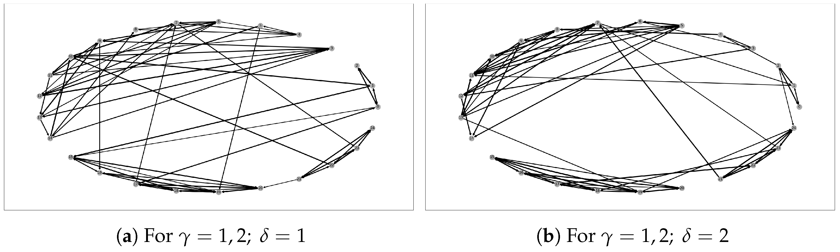
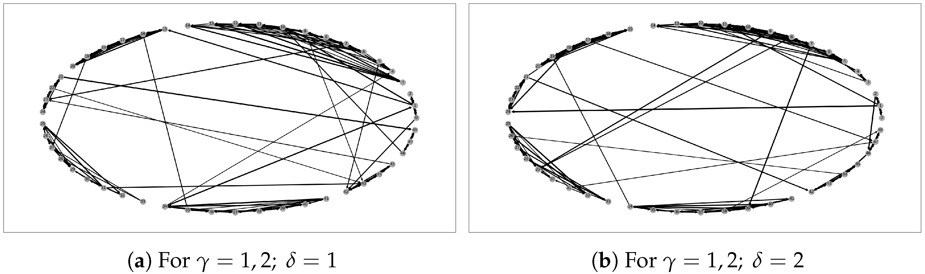
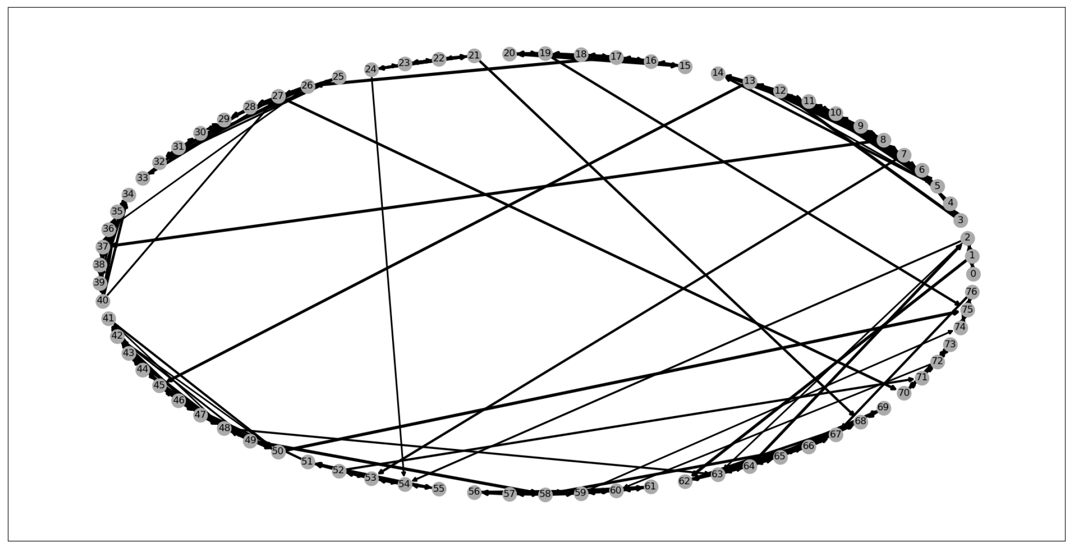
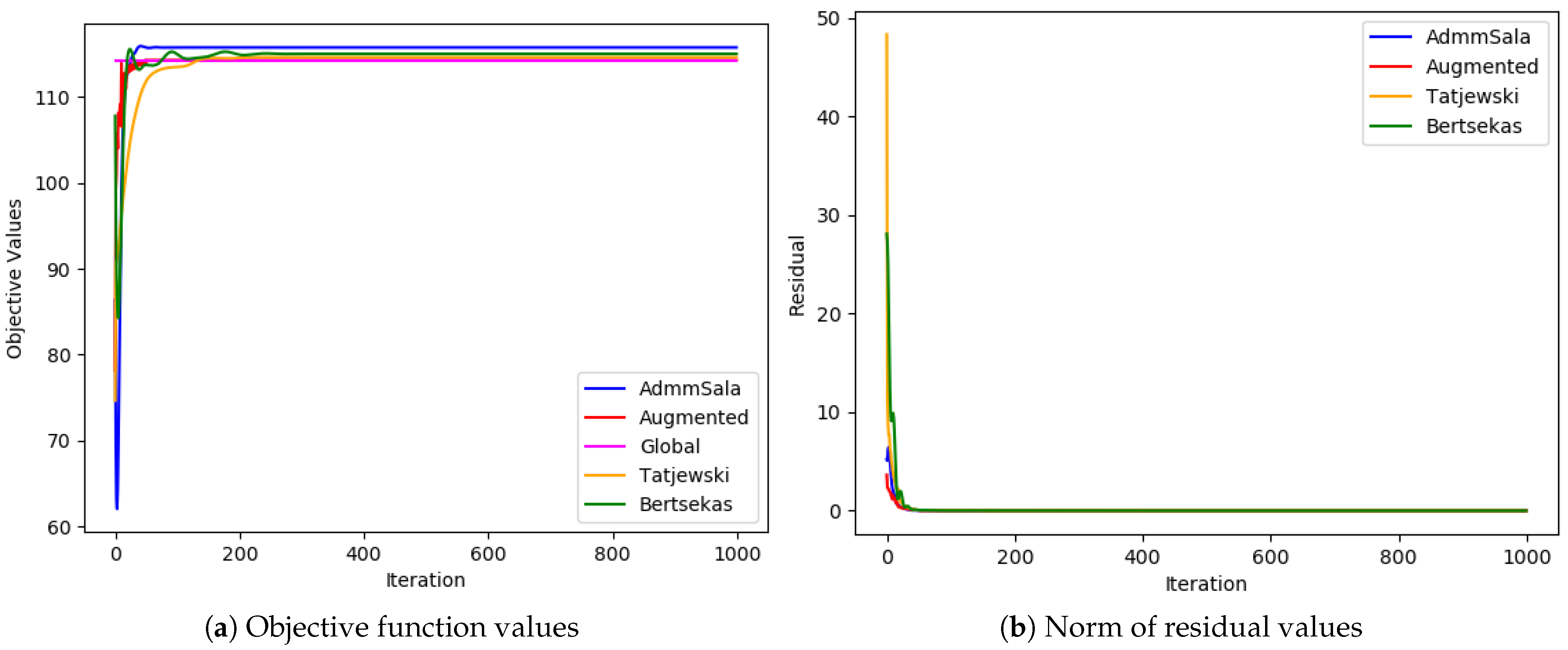
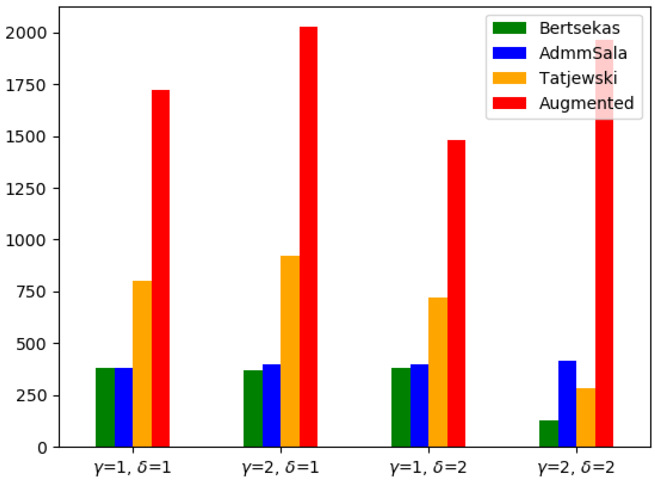
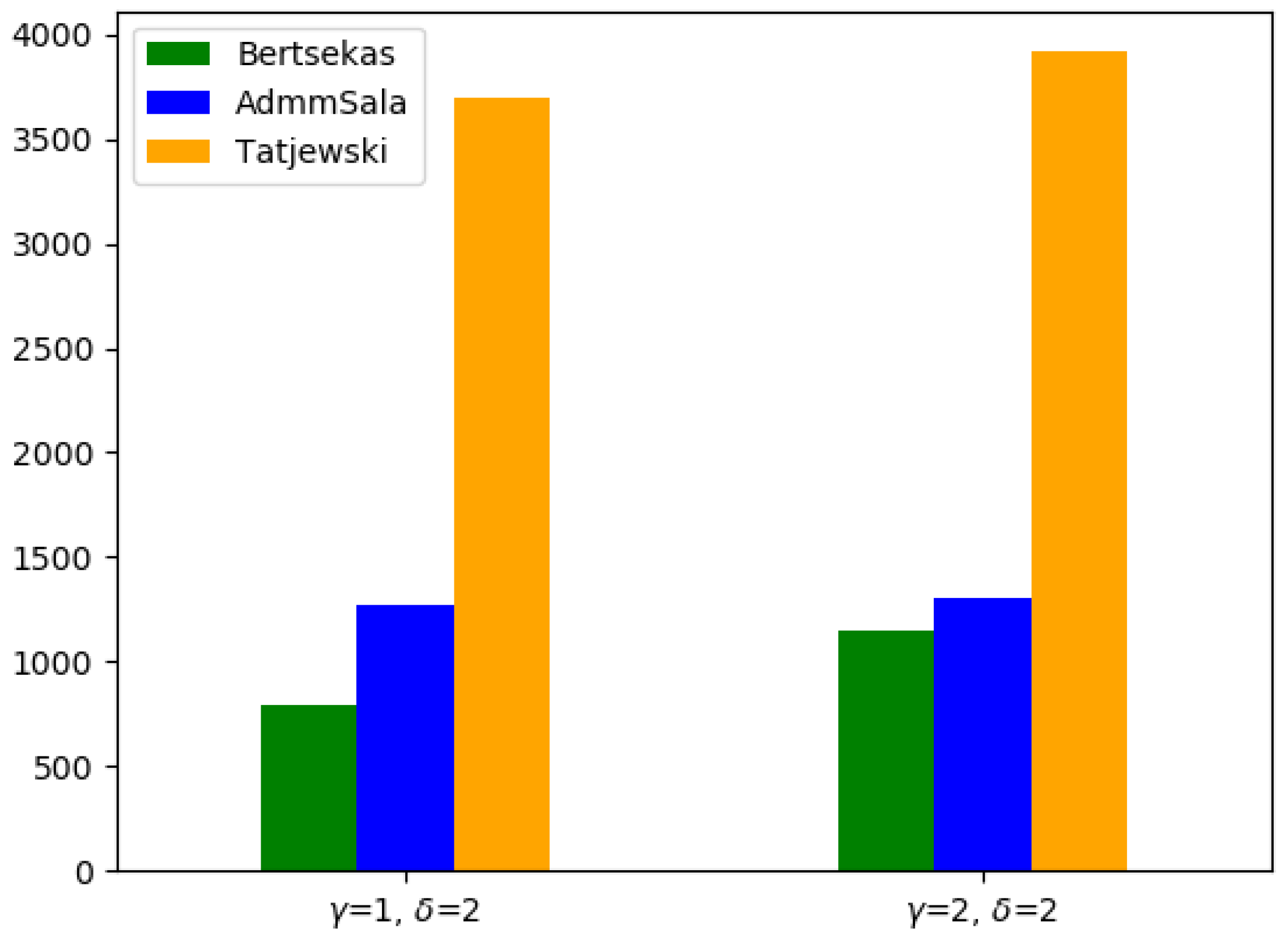
In the network problem (1)–(8), constraint binding flows (4) are of the inequality type; hence, in our version of problem formulation to be solved by the SALA algorithm (46)–(49), we introduce slack variables $z_{wl}\ge 0$, such that

$$\sum _{w\in W}{y}_{wl}-c_l+\sum _{w\in W}{z}_{wl}=\sum _{w\in W}{s}_{wl},\forall l\in L$$

(88)

where $\forall l\in L$

$$\sum _{w\in W}{s}_{wl}=0$$

(89)

Then, (88) may be written as

$$\sum _{w\in W}\left(y_{wl}-\frac{c_l}{\left|W\right|}+z_{wl}-s_{wl}\right)=0$$

(90)

The equality constraint for the flow $w\in W$ in link $l\in L$ will be as follows:

$$y_{wl}-\frac{c_l}{\left|W\right|}+z_{wl}-s_{wl}=0$$

(91)

The augmented Lagrangian is

$$\begin{array}{cc}\hfill L_{\rho }(x,b,y,z,s,\lambda )=& \sum _{w\in W}[f_w(x_w,b_w)\hfill \\ \hfill +& \sum _{l\in L}{\lambda }_l\left(y_{wl}-\frac{c_l}{\left|W\right|}+z_{wl}-s_{wl}\right)+\frac{\rho }{2}\sum _{l\in L}{\left(y_{wl}-\frac{c_l}{\left|W\right|}+z_{wl}-s_{wl}\right)}^2]\hfill \\ \hfill =& \sum _{w\in W}\left[f_w(x_w,b_w)+L_{pen,{\rho }_w}(y_w,s_w,z,\lambda )\right]\hfill \\ \hfill \triangleq & \sum _{w\in W}{L}_{{\rho }_w}(x_w,b_w,y_w,s_w,z,\lambda )\hfill \end{array}$$

(92)

where

$$L_{pen,{\rho }_w}(y_w,s_w,z,\lambda )=\sum _{l\in L}\left[{\lambda }_l\left(y_{wl}-\frac{c_l}{\left|W\right|}+z_{wl}-s_{wl}\right)+\frac{\rho }{2}{\left(y_{wl}-\frac{c_l}{\left|W\right|}+z_{wl}-s_{wl}\right)}^2\right]$$

(93)

The algorithm (55)–(59) adapted to this problem will take the form

$$\begin{array}{ccc}\hfill & (x_w^{k+1},b_w^{k+1},y_w^{k+1},z_w^{k+1})& =arg\underset{\begin{array}{c}(x_w,b_w,y_w)\in XB{Y}_w\\ z\ge 0\end{array}}{min}{L}_{{\rho }_w}(x_w,b_w,y_w,z,s_w^k,{\lambda }^k),w\in W\hfill \end{array}$$

(94)

$$\begin{array}{ccc}& \mathrm{C}\mathrm{a}\mathrm{l}\mathrm{c}\mathrm{u}\mathrm{l}\mathrm{a}\mathrm{t}\mathrm{e}{r}_l^{k+1}& =\sum _{w\in W}\left(y_{wl}^{k+1}+z_{wl}^{k+1}\right)-c_l,l\in L\hfill \end{array}$$

(95)

$$\begin{array}{ccc}& s^{k+1}& =y_{wl}-\frac{c_l}{\left|W\right|}+z_{wl}-\frac{r_l}{\left|W\right|}\hfill \end{array}$$

(96)

$$\begin{array}{ccc}& {\lambda }_l^{k+1}& ={\lambda }_l^k+\frac{{\rho }_k}{\left|W\right|}{r}_l^{k+1},w\in W,l\in L\hfill \end{array}$$

(97)

$$\begin{array}{ccc}& {\rho }_{k+1}& =\alpha {\rho }_k,\alpha \ge 1\hfill \end{array}$$

(98)

6. Numerical Tests

The algorithms described above were implemented and tested on ten network problems of different sizes. The tested networks consisted of loosely connected node clusters with strongly connected nodes. The problems were first solved without decomposition and later with decomposition, allowing for future parallelization (however, our tests were performed in a sequential way).

The Python 3.7.7 programming language was used for all implementations and numerical experiments. To construct and evaluate optimization problems, the amplpy software [45,46] package was employed, the Gurobi solver was used for the optimization, and the NetworkX software package [47] was applied to create and display networks related to optimization problems.

The tests were performed on the machine with AMD Ryzen 5 4600H with Radeon Graphics 3.00 GHz processor, 32 GB RAM, 64-bit operating system, x64-based processor, 512 GB SSD storage, under Windows 10 Pro operating system.

Five distinct network topologies were created for the study. The first two topologies, the medium networks, had fewer variables and can be observed in

Table 1. Problem instances.

	Number of Nodes	Number of Arcs	Number of Demands	Flow Rate Bounds	Capacity Bounds
Medium Problem	25	84	12	[0.001, 3]	[0.3, 1]
Large Problem	49	143	32	[0.001, 3]	[0.3, 1]
Extra-Large Problem	77	227	64	[0.001, 3]	[0.3, 1]

and Figure 1. The second two topologies, the large networks, had more variables and can be seen in Table 1 and Figure 2. The last topology, the extra-large network, had many more variables and can be seen in Table 1 and Figure 3. The source and destination nodes for each problem instance were generated randomly, along with the capacities of links. Instances of the problem were created for all network topologies.

Figure 4, Figure 5, Figure 6, Figure 7, Figure 8, Figure 9, Figure 10, Figure 11, Figure 12 and Figure 13 show plots of values of the objective Function (1) and the norm of constraint residuals in subsequent iterations of all optimization algorithms considered in Section 5.

In most cases, all algorithms based on the augmented Lagrangian method dealt very well with the duality gap (the biggest value of the gap was less than $5\%$; in most cases, it was below $0.5\%$), which is a serious issue when Lagrangian relaxation is applied to MINLP problems, such as simultaneous optimization of routing and bandwidth allocation [3,4,7]. Among the algorithms tested, the standard Augmented Lagrangian method achieved the objective value with the least relative error for medium and large-sized problems. In most tests, Tatjewski and ADMM SALA algorithms also produced competitive results, though slightly higher, and the Bertsekas algorithm was a little worse but not always. In the case of very-large problems, the Tatjewski algorithm proved to be the most precise, ADMM, SALA and Bertsekas algorithms were a little worse, but they all delivered approximation of solutions with a very small relative error less than $0.6\%$. The ordinary augmented Lagrangian algorithm did not converge within 8 h.

Regarding constraints violation, the algorithms are comparable—they all deliver (of course if they converge) an admissible solution with the assumed accuracy ${10}^{-6}$. As expected, none of the algorithms incurred any routing violations, indicating their ability to generate feasible routing solutions that satisfy network flow conservation equations.

The analysis of runtimes presented in

Table 2. Medium problems: Objective values and relative errors (in %) with respect to the centralized (“Global”) Gurobi solution (in brackets) for the tested AL algorithms with, respectively, $\gamma =1$ and $\delta =1$, $\gamma =2$ and $\delta =1$, $\gamma =1$ and $\delta =2$, $\gamma =2$ and $\delta =2$.

	Objective	Time (s)	Status
Global	114.31 (0.0)	0	Optimal
Augmented	114.31 (0.0)	504	Optimal
Bertsekas	115.03 (0.63)	149	Optimal
Tatjewski	114.64 (0.29)	171	Optimal
AdmmSala	115.78 (1.29)	87	Optimal
Global	191.61 (0.0)	1	Optimal
Augmented	191.61 (0.0)	976	Optimal
Bertsekas	195.45 (2.0)	162	Optimal
Tatjewski	191.63 (0.01)	368	Optimal
AdmmSala	196.55 (2.58)	85	Optimal
Global	163.26 (0.0)	0	Optimal
Augmented	163.26 (0.0)	93	Optimal
Bertsekas	163.42 (0.1)	44	Optimal
Tatjewski	170.75 (4.59)	216	Optimal
AdmmSala	163.26 (0.0)	84	Optimal
Global	246.52 (0.0)	2	Optimal
Augmented	246.52 (0.0)	137	Optimal
Bertsekas	247.74 (0.49)	95	Optimal
Tatjewski	246.5 (0.01)	222	Optimal
AdmmSala	246.55 (0.01)	85	Optimal

,

Table 3. Large problems: Objective values and relative errors (in %) with respect to the centralized (“Global”) Gurobi solution (in brackets) for the tested AL algorithms with, respectively, $\gamma =1$ and $\delta =1$, $\gamma =2$ and $\delta =1$, $\gamma =1$ and $\delta =2$, $\gamma =2$ and $\delta =2$.

	Objective	Time (s)	Status
Global	384.96 (0.0)	4005	Timeout
Augmented	384.96 (0.0)	1723	Optimal
Bertsekas	385.09 (0.03)	379	Optimal
Tatjewski	384.98 (0.0)	800	Optimal
AdmmSala	385.32 (0.09)	383	Optimal
Global	632.92 (0.0)	4003	Timeout
Augmented	632.92 (0.0)	2026	Optimal
Bertsekas	635.18 (0.36)	369	Optimal
Tatjewski	632.95 (0.0)	920	Optimal
AdmmSala	633.67 (0.12)	396	Optimal
Global	570.92 (0.0)	4007	Timeout
Augmented	570.92 (0.0)	1482	Optimal
Bertsekas	571.49 (0.1)	379	Optimal
Tatjewski	570.91 (0.0)	718	Optimal
AdmmSala	571.06 (0.03)	395	Optimal
Global	819.84 (0.0)	4006	Timeout
Augmented	819.84 (0.0)	1965	Optimal
Bertsekas	820.57 (0.09)	127	Optimal
Tatjewski	820.36 (0.06)	280	Optimal
AdmmSala	820.16 (0.04)	416	Optimal

and

Table 4. Extra-large problems: Objective values and relative errors (in %) with respect to the centralized (“Global”) Gurobi solution (in brackets) for the tested AL algorithms with, respectively, $\gamma =1$ and $\delta =2$, $\gamma =2$ and $\delta =2$.

	Objective	Time (s)	Status
Global	1123.49 (0.0)	6013	Timeout
Augmented	1153.63 (2.68)	30,938	MaxIter
Bertsekas	1124.75 (0.11)	796	Optimal
Tatjewski	1124.0 (0.05)	3692	Optimal
AdmmSala	1125.1 (0.14)	1268	Optimal
Global	1627.31 (0.0)	30,042	Timeout
Augmented	1682.76 (3.41)	31,040	MaxIter
Bertsekas	1635.12 (0.48)	1147	Optimal
Tatjewski	1632.81 (0.34)	3917	Optimal
AdmmSala	1636.19 (0.55)	1302	Optimal

and Figure 14, Figure 15 and Figure 16 reveals that while the medium problems are solved very fast by one of the best commercial solvers (Gurobi), in the case of large problems, AL-based decomposed algorithms are competitive. The run times of delivering of a good approximation of the optimal solution were 2–3 times shorter for the standard AL algorithm and 4–14 (for one test example even 31.5) times for the algorithms with decomposition. In the case of very large problems the decomposed algorithms were 1.6–26 times faster than Gurobi solver. The standard augmented Lagrangian method required significantly more time to solve both medium and large-sized problems and failed in the case of very-large problems.

The results highlight the trade-offs between various Lagrangian-based optimization algorithms. The standard augmented Lagrangian excels in finding optimal routing solutions in not-too-big problems but at the cost of increased computational time. The Bertsekas algorithm offers a balanced approach, achieving competitive results with shorter runtimes. Tatjewski’s algorithm maintains high accuracy of solutions for big problems, making it suitable for scenarios with stringent demands. For very big problems ADMM SALA is a little worse in terms of the objective function, but it is quite fast.

It should be mentioned that the above AL-based methods will work also for more complicated two-layer network problems, e.g., with logarithmic objective functions [3].

7. Conclusions

We have discussed several algorithms for solving separable, mixed-integer, problems in a decomposed way and implemented them using Python and amplpy. We have tested these implementations on a network optimization problem of simultaneous routing and bandwidth allocation.

Since this network optimization problem has inequality constraints that bind subproblems, while in the original presentations of these methods, the binding constraints were equalities, we reformulated them.

Based on the results of numerical experiments we can conclude that all augmented Lagrangian-based algorithms (standard, Bertsekas, Tatjewski and SALA) overcome the duality gap, which is a serious disadvantage of using the Lagrangian Relaxation method to solve the two-layer routing and bandwidth allocation problem with single paths [3,4,7]. They deliver a very good approximation of the exact optimal solution in a relatively short time, usually 4–10 times shorter than that of the exact commercial solvers.

Applying parallelization to solve independently local optimization problems for particular flows should give additional speed up of the decomposed algorithms.

The choice of a particular AL-based optimization algorithm should be tailored to the specific requirements of the network problem. Standard augmented Lagrangian stands out as the go-to choice for small problems. The Bertsekas method offers a strong compromise between solution quality and runtime efficiency, and hence, it is suitable for large-scale problems where decomposition is needed, while the Tatjewski method excels in the solution quality. Ultimately, the selection of the algorithm should align with the priorities of the network optimization problem at hand.

Our formal analysis sheds light on the mathematical difficulties of Lagrangian-based optimization algorithms in the context of two-layer network problems, providing some insights for practitioners and researchers in the field of information technology and network optimization.

Our future works on simultaneous routing and bandwidth allocation problem in energy-aware networks will concern different than quadratic QoS components of the objective function (e.g., logarithmic [3]), nonseparable problems and more complicated models of the cost of energy, including unidirectional links.

References

1. Data Centres and Data Transmission Networks. Available online: https://www.iea.org/reports/data-centres-and-data-transmission-networks (accessed on 12 February 2024).
2. Koot, M.; Wijnhoven, F. Usage impact on data center electricity needs: A system dynamic forecasting model. Appl. Energy 2021, 291, 116798. [Google Scholar] [CrossRef]
3. Jaskóła, P.; Arabas, P.; Karbowski, A. Simultaneous routing and flow rate optimization in energy-aware computer networks. Int. J. Appl. Math. Comput. Sci. 2016, 26, 231–243. [Google Scholar] [CrossRef]
4. Wang, J.; Li, L.; Low, S.H.; Doyle, J.C. Cross-layer optimization in TCP/IP networks. IEEE/ACM Trans. Netw. 2005, 13, 582–595. [Google Scholar] [CrossRef]
5. Jünger, M.; Liebling, T.; Naddef, D.; Nemhauser, G.; Pulleyblank, W.; Reinelt, G.; Rinaldi, G.; Wolsey, L.A. (Eds.) 50 Years of Integer Programming 1958–2008: From the Early Years to the State-of-the-Art; Springer: Berlin/Heidelberg, Germany, 2010. [Google Scholar]
6. Li, D.; Sun, X. Nonlinear Integer Programming; Springer: New York, NY, USA, 2006. [Google Scholar]
7. Ruksha, I.; Karbowski, A. Decomposition Methods for the Network Optimization Problem of Simultaneous Routing and Bandwidth Allocation Based on Lagrangian Relaxation. Energies 2022, 15, 7634. [Google Scholar] [CrossRef]
8. Rockafellar, R. Augmented Lagrange multiplier functions and duality in nonconvex programming. SIAM J. Control. 1974, 12, 268–285. [Google Scholar] [CrossRef]
9. Huang, X.; Yang, X. Duality and Exact Penalization via a Generalized Augmented Lagrangian Function. In Optimization and Control with Applications; Qi, L., Teo, K., Yang, X., Eds.; Springer: Boston, MA, USA, 2005; pp. 101–114. [Google Scholar]
10. Huang, X.; Yang, X. Further study on augmented Lagrangian duality theory. J. Glob. Optim. 2005, 31, 193–210. [Google Scholar] [CrossRef]
11. Burachik, R.S.; Rubinov, A. On the absence of duality gap for Lagrange-type functions. J. Ind. Manag. Optim. 2005, 1, 33–38. [Google Scholar] [CrossRef]
12. Nedich, A.; Ozdaglar, A. A geometric framework for nonconvex optimization duality using augmented lagrangian functions. J. Glob. Optim. 2008, 40, 545–573. [Google Scholar] [CrossRef]
13. Boland, N.; Eberhard, A. On the augmented Lagrangian dual for integer programming. Math. Program. 2015, 150, 491–509. [Google Scholar] [CrossRef]
14. Gu, X.; Ahmed, S.; Dey, S.S. Exact augmented lagrangian duality for mixed integer quadratic programming. SIAM J. Optim. 2020, 30, 781–797. [Google Scholar] [CrossRef]
15. Bertsekas, D.P. Constrained Optimization and Lagrange Multiplier Methods; Academic Press: New York, NY, USA, 1982. [Google Scholar]
16. Bertsekas, D.P. Multiplier methods: A survey. Automatica 1976, 12, 133–145. [Google Scholar] [CrossRef]
17. Wierzbicki, A.P. A penalty function shifting method in constrained static optimization and its convergence properties. Arch. Autom. I Telemech. 1971, 16, 395–416. [Google Scholar]
18. Stein, O.; Oldenburg, J.; Marquardt, W. Continuous reformulations of discrete-continuous optimization problems. Comput. Chem. Eng. 2004, 28, 1951–1966. [Google Scholar] [CrossRef]
19. Bragin, M.A.; Luh, P.B.; Yan, B.; Sun, X. A scalable solution methodology for mixed-integer linear programming problems arising in automation. IEEE Trans. Autom. Sci. Eng. 2019, 16, 531–541. [Google Scholar] [CrossRef]
20. Chen, Y.; Guo, Q.; Sun, H. Decentralized unit commitment in integrated heat and electricity systems using sdm-gs-alm. IEEE Trans. Power Syst. 2019, 34, 2322–2333. [Google Scholar] [CrossRef]
21. Cordova, M.; Oliveira, W.d.; Sagastizábal, C. Revisiting augmented Lagrangian duals. Math. Program. 2022, 196, 235–277. [Google Scholar] [CrossRef]
22. Liu, Z.; Stursberg, O. Distributed Solution of Mixed-Integer Programs by ADMM with Closed Duality Gap. In Proceedings of the IEEE Conference on Decision and Control, Cancun, Mexico, 6–9 December 2022; pp. 279–286. [Google Scholar] [CrossRef]
23. Hong, M. A distributed, asynchronous, and incremental algorithm for nonconvex optimization: An ADMM approach. IEEE Trans. Control Netw. Syst. 2018, 5, 935–945. [Google Scholar] [CrossRef]
24. Lin, Z.; Li, H.; Fang, C. Alternating Direction Method of Multipliers for Machine Learning; Springer: Singapore, 2022. [Google Scholar]
25. Bertsekas, D.P. Convexification procedures and decomposition methods for nonconvex optimization problems. J. Optim. Theory Appl. 1979, 29, 169–197. [Google Scholar] [CrossRef]
26. Tanikawa, A.; Mukai, H. A new technique for nonconvex primal-dual decomposition of a large-scale separable optimization problem. IEEE Trans. Autom. Control 1985, 30, 133–143. [Google Scholar] [CrossRef]
27. Tatjewski, P. New dual-type decomposition algorithm for nonconvex separable optimization problems. Automatica 1989, 25, 233–242. [Google Scholar] [CrossRef]
28. Tatjewski, P.; Engelmann, B. Two-level primal-dual decomposition technique for large-scale nonconvex optimization problems with constraints. J. Optim. Theory Appl. 1990, 64, 183–205. [Google Scholar] [CrossRef]
29. Hamdi, A.; Mahey, P.; Dussault, J.P. A New Decomposition Method in Nonconvex Programming Via a Separable Augmented Lagrangian. In Recent Advances in Optimization; Gritzmann, P., Horst, R., Sachs, E., Tichatschke, R., Eds.; Springer: Berlin/Heidelberg, Germany, 1997; pp. 90–104. [Google Scholar]
30. Sun, K.; Sun, X.A. A two-level distributed algorithm for nonconvex constrained optimization. Comput. Optim. Appl. 2023, 84, 609–649. [Google Scholar] [CrossRef]
31. Houska, B.; Frasch, J.; Diehl, M. An Augmented Lagrangian Based Algorithm for Distributed Nonconvex Optimization. SIAM J. Optim. 2016, 26, 1101–1127. [Google Scholar] [CrossRef]
32. Boland, N.; Christiansen, J.; Dandurand, B.; Eberhard, A.; Oliveira, F. A parallelizable augmented Lagrangian method applied to large-scale non-convex-constrained optimization problems. Math. Program. 2019, 175, 503–536. [Google Scholar] [CrossRef]
33. Kuhn, H.W.; Tucker, A.W. Nonlinear programming. In Proceedings of the Second Berkeley Symposium on Mathematical Statistics and Probability; Neyman, J., Ed.; University of California Press: Berkeley, CA, USA, 1951; Volume 2, pp. 481–492. [Google Scholar]
34. Arrow, K.J.; Hurwicz, L. Reduction of constrained maxima to saddlepoint problems. In Proceedings of the Third Berkeley Symposium on Mathematical Statistics and Probability; Neyman, J., Ed.; University of California Press: Berkeley, CA, USA, 1956; Volume 5, pp. 1–20. [Google Scholar]
35. Arrow, K.; Hurwicz, L.; Uzawa, H. Studies in Linear and Nonlinear Programming; Stanford Mathematical Studies in the Social Sciences; Stanford University Press: Redwood City, CA, USA, 1958. [Google Scholar]
36. Powell, M.J.D. A Method for Nonlinear Constraints in Minimization Problems; Fletcher, R., Ed.; Optimization, Academic Press: New York, NY, USA, 1969; pp. 283–298. [Google Scholar]
37. Hestenes, M.R. Multiplier and gradient methods. J. Optim. Theory Appl. 1969, 4, 303–320. [Google Scholar] [CrossRef]
38. Fletcher, R. A class of methods for nonlinear programming with termination and convergence properties. In Integer and Nonlinear Programming; Abadie, J., Ed.; North-Holland: Amsterdam, The Netherland, 1970; pp. 157–173. [Google Scholar]
39. Mukai, H.; Polak, E. A quadratically convergent primal-dual algorithm with global convergence properties for solving optimization problems with equality constraints. Math. Program. 1975, 9, 336–349. [Google Scholar] [CrossRef]
40. Bertsekas, D.P.; Tsitsiklis, J.N. Parallel and Distributed Computation: Numerical Methods; Prentice Hall Inc.: Englewood Cliffs, NJ, USA, 1989. [Google Scholar]
41. Glowinski, R.; Marroco, A. On the approximation, by finite elements of order one, and the resolution, by penalization-duality of a class of non-Dirichlet problems linéaires. Math. Model. Numer. Anal. Math. Model. Numer. Anal. 1975, 9, 41–76. [Google Scholar]
42. Gabay, D.; Mercier, B. A dual algorithm for the solution of nonlinear variational problems via finite element approximation. Comput. Math. Appl. 1976, 2, 17–40. [Google Scholar] [CrossRef]
43. Hamdi, A. Two-level primal-dual proximal decomposition technique to solve large scale optimization problems. Appl. Math. Comput. 2005, 160, 921–938. [Google Scholar] [CrossRef]
44. Hamdi, A.; Mishra, S.K. Decomposition methods based on augmented lagrangians: A survey. In Topics in Nonconvex Optimization: Theory and Applications; Springer: New York, NY, USA, 2011; Volume 50, pp. 175–203. [Google Scholar] [CrossRef]
45. AMPL Optimization Inc.—Amplpy: Python API for AMPL. Available online: https://github.com/ampl/amplpy/ (accessed on 21 February 2024).
46. Fourer, R.; Gay, D.M.; Kernighan, B.W. AMPL: A Modeling Language For Mathematical Programming, 2nd ed.; Duxbury Press: Belmont, CA, USA, 2003; Available online: https://ampl.com/resources/the-ampl-book/ (accessed on 21 February 2024).
47. NetworkX—Network Analysis in Python. Available online: https://networkx.org/ (accessed on 12 February 2024).
Figure 1. Medium network topology.
Energies 17 01233 g001
Figure 2. Large network topology.
Energies 17 01233 g002
Figure 3. Extra-large network topology for γ = 1 , 2 ; δ = 2 .
Energies 17 01233 g003
Figure 4. Medium problem ( γ = 1 and δ = 1 ).
Energies 17 01233 g004
Figure 5. Medium problem ( γ = 2 and δ = 1 ).
Energies 17 01233 g005
Figure 6. Medium problem ( γ = 1 and δ = 2 ).
Energies 17 01233 g006
Figure 7. Medium problem ( γ = 2 and δ = 2 ).
Energies 17 01233 g007
Figure 8. Large problem ( γ = 1 and δ = 1 ).
Energies 17 01233 g008
Figure 9. Large problem ( γ = 2 and δ = 1 ).
Energies 17 01233 g009
Figure 10. Large problem ( γ = 1 and δ = 2 ).
Energies 17 01233 g010
Figure 11. Large problem ( γ = 2 and δ = 2 ).
Energies 17 01233 g011
Figure 12. Extra-large problem ( γ = 1 and δ = 2 ).
Energies 17 01233 g012
Figure 13. Extra-large problem ( γ = 2 and δ = 2 ).
Energies 17 01233 g013
Figure 14. Run times for the Medium problems.
Energies 17 01233 g014
Figure 15. Run times for the Large problems.
Energies 17 01233 g015
Figure 16. Run times for the Extra-large problems.
Energies 17 01233 g016