Article

A Refined Wind Power Forecasting Method with High Temporal Resolution Based on Light Convolutional Neural Network Architecture

1
School of New Energy, North China Electric Power University, Beijing 102206, China
2
School of Information Engineering, Inner Mongolia University of Science and Technology, Baotou 014010, China
*
Author to whom correspondence should be addressed.
Energies 2024, 17(5), 1183; https://doi.org/10.3390/en17051183
Submission received: 26 January 2024 / Revised: 27 February 2024 / Accepted: 28 February 2024 / Published: 1 March 2024
(This article belongs to the Section A3: Wind, Wave and Tidal Energy)

Abstract

:
With a large proportion of wind farms connected to the power grid, it brings more pressure on the stable operation of power systems in shorter time scales. Efficient and accurate scheduling, operation control and decision making require high time resolution power forecasting algorithms with higher accuracy and real-time performance. In this paper, we innovatively propose a high temporal resolution wind power forecasting method based on a light convolutional architecture—DC_LCNN. The method starts from the source data and novelly designs the dual-channel data input mode to provide different combinations of feature data for the model, thus improving the upper limit of the learning ability of the whole model. The dual-channel convolutional neural network (CNN) structure extracts different spatial and temporal constraints of the input features. The light global maximum pooling method replaces the flat operation combined with the fully connected (FC) forecasting method in the traditional CNN, extracts the most significant features of the global method, and directly performs data downscaling at the same time, which significantly improves the forecasting accuracy and efficiency of the model. In this paper, the experiments are carried out on the 1 s resolution data of the actual wind field, and the single-step forecasting task with 1 s ahead of time and the multi-step forecasting task with 1~10 s ahead of time are executed, respectively. Comparing the experimental results with the classical deep learning models in the current field, the proposed model shows absolute accuracy advantages on both forecasting tasks. This also shows that the light architecture design based on simple deep learning models is also a good solution in performing high time resolution wind power forecasting tasks.

1. Introduction

With a large proportion of wind farms connected to the grid, wind energy has a more significant impact on the operation and decision making of a power system in multiple scenarios due to its own randomness and volatility. High-performance wind power forecasting technology is becoming more and more critical to ensure the safe and stable operation of power systems [1]. In the operation of wind farms, wind power forecasting can help wind farms optimize their power generation plans and reasonably arrange the operation and scheduling of wind turbines according to the forecast result in order to maximize power generation and revenue. Accurate wind energy forecasting can help wind farms plan scheduling, operation and maintenance programs and predict adverse weather conditions such as low or high wind speeds, so that timely measures can be taken to ensure the safe operation of wind turbines. Through accurate wind energy forecasting, wind farms can better control power generation and avoid low-load operations or overload operations, thus saving O&M (operations and maintenance) costs and expenses; in terms of power system operation, wind energy forecasting is very important for the scheduling and balancing of a power system. Forecasting wind power output can help power system operators rationally dispatch other generating units to ensure the balance of supply and demand in the power system. Accurate wind energy forecasts can improve the reliability and stability of the power system, avoiding changes in the power system frequency and voltage caused by wind power changes and thus ensuring the stable operation of the power system. Wind energy forecasting can provide important references for energy planning and market operation, help decision makers to rationally plan and arrange the access and dispatch of wind power, and improve the utilization rate and market competitiveness of renewable energy. In addition, wind power forecasts can help reduce dependence on traditional fossil energy sources, reduce greenhouse gas emissions, and promote the sustainable development of sustainable energy sources.
Power systems operate under different time scales. Application scenarios under different time scales have different requirements for the accuracy and timeliness of wind power forecasting results. Wind power forecasting techniques can be categorized by time scales: ultra-short-term forecasts (seconds to 30 min in advance), short-term forecasts (30 min to 6 h in advance), medium-term forecasts (6 h to 1 day in advance), and long-term forecasts (1 day to 1 week or longer in advance) [2,3,4]. Ultra-short-term and short-term wind power forecasts: Accurate ultra-short-term and short-term forecasting can help utilities optimize generation schedules, adjust load balancing, and reduce reliance on backup generation equipment. In addition, short-term forecasting can help power market participants make more accurate power trading decisions and improve market efficiency. Medium-term wind forecasting: this helps power companies assess the potential and feasibility of wind farms and formulate reasonable power generation plans, among other things. Long-term wind energy forecasting: this can help governments and energy companies assess the long-term trend of wind energy resources, identify suitable locations for wind farm construction, and formulate sustainable energy development strategies.
There are also specific application scenarios in the power system that require high-resolution wind power forecasting technology as a technical support. Power system frequency regulation: The power system needs to maintain a balance between supply and demand to ensure a stable power supply. Second- and minute-level wind power forecasting can be used for scheduling and controlling the output of wind farms to meet the requirements of system frequency regulation and scheduling. Wind farm model predictive control: Wind farm model predictive control is a model-based control strategy that optimizes the operation strategy of wind farms by predicting the future wind power in order to maximize the energy output or reduce the impact on the power system. The active and reactive power regulation of a wind turbine can be mechanically adjusted, on the one hand, by the blade pitch angle and yaw angle. On the other hand, the torque output and power factor angle of the converter can be adjusted. The former can be adjusted in seconds or even tens of seconds. The latter can be adjusted electromagnetically in ms. For example, the SVC/SVG reactive power regulation time is 50–200 ms for SVCs and 20–100 ms for SVGs, while the reactive power regulation time of wind turbines is between 1 and10 s. In this paper, the results of wind power prediction are presented. It is intended to be used for lower levels of the electromagnetic regulation of wind turbines. Therefore, the method of wind power prediction in seconds is used [5]. Second- and minute-level wind power forecasting can provide accurate inputs to help optimize the control strategy of a wind farm. Short-term market trading: Short-term trading in the electricity market requires accurate wind power forecasts in order to participate in the market and to develop appropriate strategies for buying and selling electricity. Second- and minute-scale forecasting can provide wind power information on finer time scales to help power system operators and participants make more timely and accurate decisions to improve system efficiency and reliability [6].
From the above application scenarios of power systems with different time scales, it can be seen that the smaller the time scale is, the higher the accuracy and timeliness of wind power prediction results required. Currently, most of the existing research focuses on ultra-short-term (minutes to hours), short-term (hours to days), and medium-to-long-term (days to months) wind power prediction techniques, while research on ultra-ultra-short-term (seconds) wind power forecasting is still rare. With a large proportion of wind energy penetrating the power grid, which puts more pressure on the stable operation of the power grid in shorter time scales, wind farms need finer real-time wind power forecasting results for efficient scheduling and operation control decisions, and therefore, we need to study high time resolution forecasting algorithms with higher accuracy and real-time performance.
Wind power forecasting methods can be categorized by model theory as physically based [7], statistically based [8], machine learning-based methods [9], and hybrid methods [10,11]. Deep learning belongs to a branch of machine learning methods. With the development of data collection equipment and communication technology, the huge amount of system data owned by wind farms provides greater possibilities for the further application of deep learning methods in the field of wind power forecasting. A large number of scholars have already achieved fruitful research results on wind power forecasting techniques based on deep learning. Currently, the more commonly used classical deep learning methods in this field are recurrent neural networks (RNNs) [12], long short-term memory networks (LSTMs) [13], and convolutional neural networks (CNNs) [14].
RNN is limited in its ability to learn long-term dependent features because of the gradient explosion or disappearance that can easily occur during the training process. LSTM, a variant structure of RNN, mitigates the degree of gradient explosion and disappearance of RNN and enhances the ability of RNN to deal with long time problems by setting up long-term memory units and gating mechanisms. So, it is increasingly used in the field of wind power forecasting. The literature [15] proposes a bi-directional LSTM based on wavelet neural networks for ultra-short-term wind voltaic power forecasting. The wavelet neural network is utilized to weigh the importance of historical information so that the LSTM hidden layer states are given different weights to improve the prediction accuracy.
The literature [16] proposed an LSTM network model with an enhanced forgetting gate, LSTM-EFG, which solves the problems of gradient vanishing and gradient explosion, to a certain extent, improves the ability of the model to extract long-term dependencies, and significantly improves its forecasting accuracy compared with standard LSTM. The literature [17] came out with an improved forecasting method based on the long short-term memory (LSTM) network, developed the multiple imputation technique (MIT) to reconstruct the data and utilized it for filling missing samples, and then applied LSTM to extract the long-term trend afterwards, which achieved better forecasting results. All of the LSTM-based methods described above have, to some extent, improved the ability of the model to extract long-term dependent feature relationships, while the ability to obtain spatial features of wind power data is still limited, and the model running time is long [18,19,20].
The CNN is one of the mainstream deep learning methods, which is inspired by the biological visual system, and it extracts features from images by simulating the way of human visual processing. The core idea of the CNN is to construct a network structure by using convolutional and pooling layers, and its advantage lies in its local perceptual and weight sharing mechanism, which makes it perform well on data with local structures, and it has high computational efficiency due to the ability of parallel computation. The CNN is widely used in computer vision, natural language processing, and time series analysis. In recent years, it has been increasingly applied to the field of wind power forecasting. The literature [21] proposes a novel ensemble wind power forecasting method based on the CNN, which is applied to the task of short-term wind power probabilistic forecasting. The raw wind power data are decomposed into feature data of different frequencies using wavelet transform, and then a convolutional neural network is used to learn the nonlinear features in each frequency feature data. Experiments demonstrate that the method can better learn the uncertainty in wind power data and achieve high forecasting accuracy. The literature [22] introduces a novel CNN-based deep neural network (WSFNet) for short-term multi-step wind speed forecasting. The model is based on a stacked convolutional neural network (CNN), which establishes feature mapping between the inputs and the convolutional blocks by means of a channel attention module and a densely connected layer. The method ultimately achieves a good forecasting performance and can be effectively used for smart grid operation. Given the respective advantages of the CNN and LSTM, scholars have applied the combination of both to wind power forecasting tasks. The literature [23] proposed a CNN_LSTM forecasting model combined with a swarm intelligence (SI) optimization algorithm to perform a short-term offshore wind power forecasting task, and the experimental results provided accurate wind power prediction data for the management of renewable energy conversion networks. The literature [24] proposed a deep learning model based on CNN-Bi-LSTM and embedded GA optimization for forecasting wind speed for the next 24 h. The internal features of the time series are directly extracted using the CNN, while the Bi-LSTM can fully utilize the upper layer information from both forward and backward directions. The proposed method shows better performance than other methods.
In addition, the specific structure and parameter settings of CNNs can be adapted and optimized for different tasks and datasets. Gradually new CNN variants have been applied to wind power forecasting recently. The literature [25] introduces an attention mechanism based on a variant of the CNN structure (causal convolutional network [26]) instead of a dot product attention mechanism, focusing on the important spatio-temporal information of the input data, and then utilizes the coding and decoding structure of the current state-of-the-art transformer model [27] to extract the long-term dependencies, which enhances the interpretability of the model while achieving a better forecasting performance than commonly used prediction methods. The literature [28] proposes a short-term wind power forecasting method based on time convolutional neural networks [29]. The wind power time series are separated by the empirical modal decomposition method and then used as the input to the residual correction model based on the temporal convolutional network to predict the wind power residuals, which achieves a better forecasting performance. In recent years, many improved CNN models, such as ResNet, Inception, and MobileNet [30], have also emerged for further improving the performance of image recognition and computer vision tasks. The literature [31] proposes a deep neural network model using ResNet architecture applied to short- and medium-term wind power forecasting, where the model utilizes ResNet modules and Inception modules to enhance the feature extraction capability. The temporal dependency between features is then further captured by a bi-directionally weighted LSTM layer and a GRU layer. The results show that the proposed model outperforms other algorithms by reducing the average absolute error by 12%.
Through the above literature research, we are inspired by the following points: most of the current research focuses on the study of wind power forecasting techniques on ultra-short and short-term time scales, and a comprehensive study of high-resolution forecasting on second-level time scales is still rare. The importance of high-resolution wind power prediction for the optimal control of active and reactive power within a wind farm site is summarized in the literature [32]. From the perspective of model input feature engineering, the input method of grouping the input data into groups by considering the in-depth fusion of the data with the model architecture and the computational mechanism is still rare. From the perspective of model architecture design, selecting applicable models for different tasks and designing model-specific architectures are also key techniques to enhance model performance. Therefore, in this study, a high-resolution refined wind power forecasting method based on a light convolutional neural network architecture, DC_LCNN, is innovatively proposed and applied to second-level high-resolution wind power forecasting. The experimental results show that the proposed method achieves a very excellent forecasting performance. The specific contributions of this study are as follows:
(1)
The input method of grouping the original input features is proposed, which provides more refined input feature information for the model through two channels with different combinations of input features.
(2)
Two parallel sets of convolutional neural networks are used to extract different kinds of feature constraint relationships: one targeted to extract local constraint relationships between wind power sequence elements, and the other considers local constraints between wind speed, wind direction, and wind power while extracting local constraint relationships between wind power sequence elements.
(3)
The light global maximum pooling approach replaces the traditional CNN’s flattening combined with the FC forecasting approach, which directly downscales the 3D feature data of the front layer, eliminating the data flattening operation and the introduction of more FC layers, which greatly improves the model’s computational efficiency.
(4)
Single-step and multi-step second-level high-resolution wind power forecasting experiments are carried out simultaneously to meet the demand for different time-scale forecasting results in high time resolution application scenarios of the power system, and the performance of the model on different average wind speed intervals is also investigated.
The remaining chapters of this paper are organized as follows: Section 2 introduces the methodology used in this study; Section 3 briefly describes the indexes used for the comprehensive performance evaluation of the forecasting results; Section 4 provides a comprehensive description of the relevant experimental details of this study and the presentation of the results; and Section 5 sums up the whole paper and gives conclusions and goals for future research.

2. Proposed Methodology

The overall research flow of the methodology proposed in this paper is shown in Figure 1. The flow is briefly described below:
1.
Data Preprocessing
Considering the deep feature learning ability of the deep learning model itself, this paper carries out basic preprocessing of the original data, including outlier removal and vacancy filling. Using min–max normalization, the data are scaled to between [0, 1] to improve the training effect and convergence speed of the model. Dimensionality changes are made to the original data to adapt to the data format requirements of the deep learning model.
2.
Input Layer
For the purpose of deeply integrating the raw data with the model structure and operation mechanism, this study innovatively designs two input data channels, which are a single wind power sequence channel and a mixed data channel of wind speed, wind power, and wind direction.
3.
Forecasting model
Considering that the task of wind power forecasting with high temporal resolution puts high demands on the timeliness and accuracy of the algorithm at the same time, this study uses a 1D CNN network as the core algorithm and innovatively designs a dual-channel light convolutional architecture.
4.
Performance evaluation and visualization
In order to objectively evaluate the prediction performance of the proposed model and increase the interpretability of the model, this paper comprehensively uses three evaluation indexes: mean absolute error (MAE), root mean square error (RMSE) coefficient of determination (R2 score), and ramp error (RE) to validate the performance of the proposed model and visualize it.

2.1. 1D Convolutional Neural Network

Moreover, 1D CNN is a variant of convolutional neural networks and is used for processing sequential data with local dependencies, such as text, audio, and time series data. Compared to traditional 2D convolutional neural networks, 1D CNN is more efficient in processing 1D data. The following is the structure and principle of 1D CNN:
Input and convolutional operations: The input to a 1D CNN is a one-dimensional sequence of data, such as a time series, a text sentence, or the waveform of an audio signal. The convolution kernel is the key component in 1D CNN, which is a sliding window with a fixed window size for extracting local features in the input sequence. Convolutional operation means sliding over the input sequence using the convolutional kernel and performing a convolution operation on the data within the window at each position. The convolution operation captures local patterns and relationships in the input sequence.
Activation function: An activation function, such as ReLU (rectified linear unit), is applied to the output of the convolution operation to introduce nonlinear transformations and enhance the expressive power of the network.
Pooling operation: Similar to 2D CNNs, 1D CNNs usually add a pooling layer after the convolutional layer. Pooling operations are used to reduce the dimensionality of the feature map and retain important feature information. Commonly used pooling operations include maximum pooling, average pooling, global average pooling, and global maximum pooling, among others.
Fully connected (FC) layers and outputs: after the convolution and pooling layers, some FC layers are usually added for mapping features to final output classes or regression values.
Furthermore, 1D CNNs need to design and adjust the structure and parameters of the model according to the specific task and data characteristics. We thus propose a light dual-channel convolutional neural network architecture (see Section 2.2) to perform the task of high time-resolved wind power forecasting.

2.2. Proposed Light Convolutional Neural Network Architecture

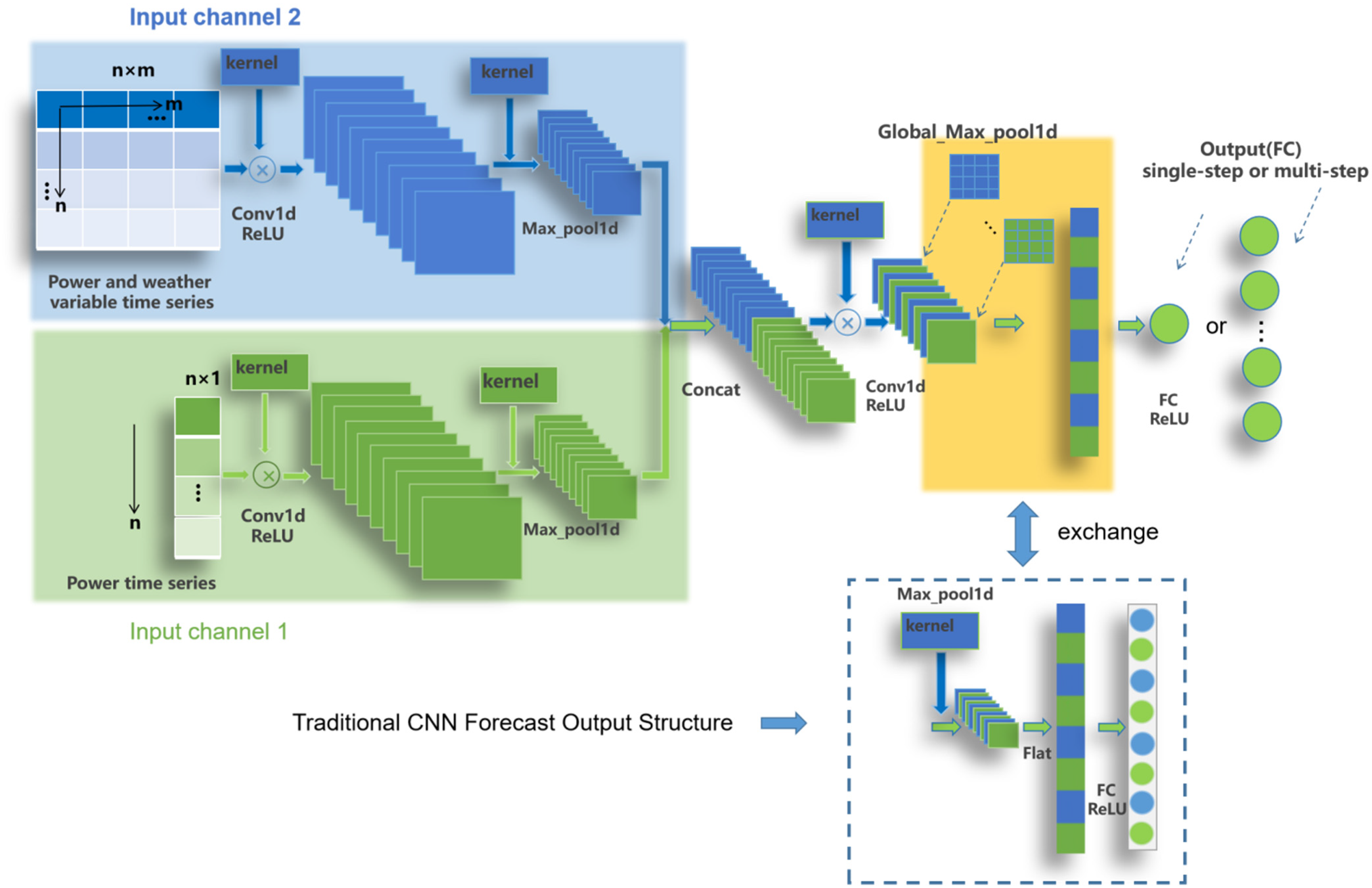
Focusing on the need for finer real-time wind power forecasting results for wind farms to make efficient scheduling and operation control decisions, this study proposes the DC_LCNN model from two aspects: the data source and the model computing mechanism and architecture. The architecture of the proposed model is shown in Figure 2.
Both a suitable model architecture and rich input feature information help to increase the upper limit of the learning ability of the deep learning model so that the model can better adapt to complex patterns and relationships. In this study, two input channels are designed to provide diverse input feature information for the model. The univariate input channel is used to provide the deep learning model with temporal feature information between elements of the wind power sequence, and the multivariate input channel is used to provide the deep learning model with spatio-temporal feature information between wind power and other meteorological variables.
Each channel uses a convolutional layer combined with a maximum pooling layer for feature extraction of the input feature information. Channel 1 first extracts the temporal dependencies between the elements of the wind power sequence through a convolutional layer and then downsizes the features and extracts the local most significant features through a maximum pooling layer while avoiding overfitting. Similarly, channel 2 also extracts the spatio-temporal constraints between the wind power sequence and other meteorological sequence elements through a convolutional layer and further extracts the local most significant spatio-temporal crossover features through a max-pooling layer; the significant feature information extracted from channels 1 and 2 is then merged as the input to the high hidden layer CNN, which is once again fused and extracted by using a convolutional layer. Subsequently, this study innovatively adopts the global maximum pooling method (yellow background region in Figure 2) instead of the traditional maximum (or average) pooling method in CNNs, and combines the flattening operation and multiple FC layers (rectangular dashed box region in Figure 2) to predict the resultant output. The global maximum pooling method is not only able to extract the most significant features globally, but also directly reduces the 3D features output from the convolutional layer to 2D feature data, avoiding overfitting while eliminating the data flattening operation. More importantly, only one FC layer with the same number of neurons as the wind power output scale is needed to directly output the forecast results, which eliminates the process of assigning weights to the upper layer features via multiple fully connected layers in the traditional CNN, simplifying the model structure and improving the computational efficiency of the model.
Finally, a light convolutional neural network architecture is built. And, a superior forecasting performance is demonstrated on single-step and multi-step high time resolution wind power forecasting tasks. The specific inputs and parameter settings of the model are described in detail in Section 4 and will not be repeated here.

3. Evaluation Indexes

In this paper, four evaluation indexes, MAE, RMSE, R2 score, and RE, are used to objectively evaluate the forecasting performance of the proposed model and to illustrate the interpretability of the model. Among them, RE is proposed to measure the consistency of the dynamic changes between the predicted sequence and the observed sequence by calculating the difference between the differential observed sequence and the differential predicted sequence. A smaller RE indicates that the predicted series can accurately model the trend of the observed series with better consistency. It is important to note that the ramp error only takes into account the trend of the series and not the overall forecast accuracy. Therefore the other three metrics above are used to fully evaluate the performance of the model. In Equation (4), Δ y i denotes the difference value of the observed series ( y i y i 1 ) and Δ y ^ i denotes the difference value of the predicted series ( y ^ i y ^ i 1 ).
M A E = 1 N t = 1 N p t p ^ t
R M S E = 1 N t = 1 N ( p t p ^ t ) 2
R 2 = 1 t ( p t p ^ t ) 2 t ( p t p ¯   p e r i o d ) 2
R E = 1 N 1 i = 2 N ( Δ y i Δ y ^ i ) 2

4. Case Study

4.1. Experimental Data

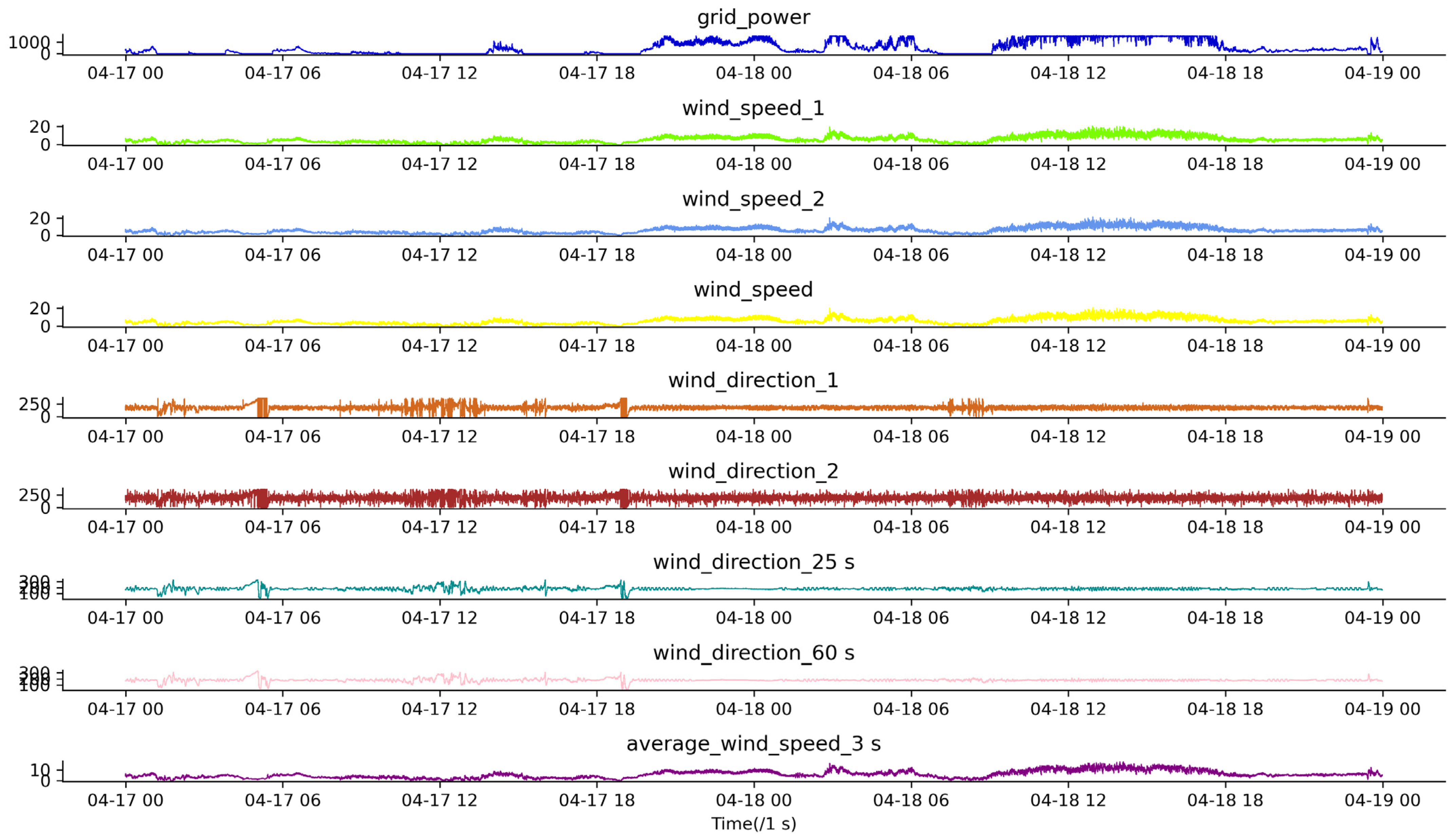
The data used in this study are two days of SCADA data from a 1.5 MW wind turbine with a time resolution of 1 s and a total of 172,800 sample points. The data contain wind power data and wind speed and direction data. Figure 3 illustrates the variation in each variable in the data over time. The ‘grid_power’ represents the current output power of the wind farm in kilowatts (kW). It is the target variables to be predicted. ‘wind_speed_1’ and ‘wind_speed_2’ represent wind speed measurements in meters per second (m/s) at two different locations in the wind farm; ‘wind_speed’ is the average of the two wind speeds; ‘wind_direction_1’ and ‘wind_direction_2’ represent wind direction measurements in degrees (°) from two different locations in the wind field; ‘wind_direction_25 s’ and ‘wind_direction_60 s’ denote the average wind direction over the past 25 s and 60 s, respectively, which can be used to capture the trend of wind direction change; and ‘average_wind_speed_3 s’ denotes the average wind speed measurement over the past 3 s and 60 s, which can be used to capture the instantaneous trend of wind speed. For the selection of feature variables used in experiments, many studies have used statistically based correlation coefficient methods (e.g., Pearson and Spearman correlation coefficient methods) to select input feature variables. Whereas some of these methods can only detect linear relationships (e.g., Pearson), some are unable to capture more complex linear relationships (e.g., Spearman), although they can detect simple nonlinear relationships (monotonic relationships). Considering the superior deep nonlinear feature extraction capability of deep learning models, this study used experimental trial and error to select the final feature combination while considering all variables. The experiment finally selected ‘grid_power’, ‘wind_speed_1’, ‘wind_speed_2’, ‘wind_speed’, ‘wind_direction_1’, ‘wind_direction_2’, ‘wind_direction_25 s’, and ‘average_wind_speed_3 s’ which are used as feature variables in the multivariate input mode for all models.

4.2. Experimental

The experiments in this study are centered around two tasks, single-step (1s ahead) and multi-step (1–10 s ahead) second-level wind power forecasting, and six experimental tasks are implemented:
In the single-step second forecasting task: (1) Channel ablation experiments of the proposed model. These are conducted to demonstrate the integrated forecasting performance of the proposed two-channel structure. (2) Experiments comparing the light convolutional structure of the proposed model with the traditional CNN structure replacement. These are conducted to demonstrate the comprehensive forecasting performance of the light convolutional structure of the proposed model. (3) Comparison experiments with classical deep learning baseline models are carried out to demonstrate the superior forecasting performance of the proposed model.
In the multi-step second forecasting task: the same three experiments as in the single-step second forecasting task experiments are performed.
The parameters of all models are obtained by trial and error. Table 1 shows the parameter settings of the proposed model for single and multi-step forecasting. “Conv1D_1(Input 1)” and “MaxPooling1D_1” represent the convolutional and maximum pooling layers in input channel 1 (green background region of Figure 2), respectively; “ Conv1D_2(Input 2)” and “MaxPooling1D_2” represent the convolutional and maximum pooling layers in input channel 2 (blue background region of Figure 2), respectively; “Conv1D_3” and “Global_MaxPooling1D_1” represent the convolutional and global maximum pooling layers in the high hidden layer (yellow background region of Figure 2), respectively. Table 2 shows the parameter settings of all baseline models for single- and multi-step forecasting. The prefix “Univar_” represents the univariate input pattern, and the prefix “Multivar_” represents the multivariate input pattern.

4.2.1. Experiments on Single-Step Second Wind Power Forecasting Task

Channel ablation experiments for the proposed model DC_LCNN were conducted. Three scenarios of using each channel independently as the only input channel to the model and both channels simultaneously as the input to the model are performed to forecast the wind power 1 s ahead, respectively. The results of the channel ablation comparison experiments are shown in Table 3, where DC1_LCNN denotes the model when channel 1 is used as the only input to the model and DC2_LCNN denotes the model when channel 2 is used as the only input to the model. It can be seen that the forecasting results of the dual-channel structure are significantly better than those when each channel acts alone. It also proves that the proposed dual-channel structure can obtain richer and more valuable feature information from the original data.
Experiments comparing the light convolutional structure of the proposed model with the traditional CNN structure replacement were conducted. The wind power forecasting is carried out using the maximum pooling method in the traditional CNN combined with the FC final forecasting structure and the global maximum pooling final forecasting structure of the proposed model, respectively, for 1 s ahead of time, and the experimental results are shown in Table 4. DC_CNN (FC) represents the two-channel model with the traditional CNN forecasting structure. It can be seen that the forecasting results of the proposed model are significantly better than those of the traditional CNN structure. The MAE was boosted by 48.37% and RMSE by 38.02%. The experiments also compare the forecasting and training time of the two structures, as shown in Table 5. The “training time” and “forecasting time” refer to the total time of all the sample points in the test set, and there are 17,280 sample points. Therefore, the average forecasting time of each step is the ratio of the forecasting time to the number of sample points in the test set. It can be seen that the proposed structure has shorter forecasting and training times. And, the forecast time of each step is by far enough to meet the time requirement of second-level application scenarios. In conclusion, the proposed light convolutional structure is significantly better than the traditional CNN structure in terms of forecasting accuracy and efficiency.
For the comparison experiments with the baseline models, we chose two sets of baseline models: the persistence model and the classical deep learning model. Table 6 gives the performance comparison results between the proposed model and the persistent model.
As can be seen from the results, on the test set chosen for this study (17,280 sample points, 4.8 h), without considering the special needs of specific application scenarios, the persistence model seems to show a better forecasting performance, with smaller MAE and RMSE, and it is worth noting that it has a large maximum absolute error. However, we still propose the DC_LCNN model for the following reasons.
First, in terms of the forecasting principle, the persistence model takes the actual value of the target variable in the previous moment as the predicted value in the next moment, which is suitable for forecasting scenarios in which short-term changes in the target variable are small and insensitive to the short-term changes in the target variable. In contrast, the second-scale wind power forecasting task carried out in this study is oriented to application scenarios with second-scale time scales such as wind farm model prediction control and frequency regulation. These scenarios are not sensitive to small variations in wind power per second intervals, and specifically in the case of small wind power changes, these real-world scenarios are not sensitive to such small errors, meaning that the prediction results of either model used do not affect the final decision, whereas these scenarios are very sensitive to large changes in wind power per second intervals. The persistence model predictions do not provide relevant changes information, which is the reason why their maximum absolute error is very large, as seen in Table 6. The proposed method in this study can more accurately forecast the change in wind power at intervals of one second.
Second, due to the limited data provided by the operator, this result is only an assessment of the wind power for 4.8 h in January, and the overall distribution of the data in this segment (roughly the segment from 18:00 April 18 to 00:00 April 19 at the end of the wind power curve in Figure 3) shows smaller changes, which is why the accuracy of the proposed model is lower than that of the persistence model.
Finally, in order to illustrate more clearly the performance of the proposed model in predicting larger wind power changes, Figure 4 gives a plot of the prediction results of the persistence model and the proposed model for larger power changes intervals against the actual measurement results. Figure 4c,d show the prediction results for the length of the 10-second intervals within the region of larger wind power changes (the part within the dashed box) in Figure 4a,b, respectively. The MAE and RMSE on the intervals corresponding to Figure 4a–d are given in Table 7, respectively. From Table 7, it can be seen that the proposed model obtains higher forecasting accuracies on both the full intervals (the intervals corresponding to Figure 4a,b and the locally zoomed intervals. The MAE and RMSE of the proposed model are improved with respect to the persistence model by 23.72% and 32.23% on the full intervals and 25.9% and 29.62% on the local zoomed-in intervals, respectively. As can be seen from Table 6, the persistence model improves the RMSE relative to the proposed model by 2.3% on the full test set. In contrast, the performance advantage of the proposed model is more obvious on the larger changes interval of wind power. It can also be visualized from Figure 4c,d that the error of the persistence model is much larger than that of the proposed model when the wind power fluctuates greatly. For example, in the power changes interval from 1 to 4 seconds, the forecast error of the persistence model is larger, and it cannot effectively forecast the large changes in wind power. The proposed model, on the other hand, can effectively forecast the changes in wind power, which is very favorable for the correct decision making in the application scenario of secondary power forecasting for wind farms.
Comparison tests with classical deep learning baseline models are carried out. In this study, several classical and commonly used deep learning models in the field, LSTM, CNN, CNN_LSTM, are used as baseline models. Each baseline model takes two input patterns, namely a univariate input pattern (only historical wind power sequence) and a multivariate input pattern (historical wind power and several other wind speed and direction sequences).
Table 8 shows the comparison results of the seven models. It can be seen that the proposed model has a clear advantage in forecasting accuracy, where the CNN with univariate input pattern has the best performance among all the baseline models. The RE of the proposed model is minimal, indicating that the proposed model is more accurate in predicting the trend of the observed series. The percentage boost in the MAE and RMSE of the proposed model with respect to each baseline model is given in Figure 5. The minimum MAE and RMSE boost percentages are 40.5% and 32.4%, respectively, which are the accuracy boosts relative to the CNN model with the univariate input pattern. It can also be seen from the experimental results that CNN obtains better forecasting performance than LSTM in the ultrashort time scale forecasting task in this study. This also indicates that CNN, due to its parallel computing mechanism, can use the convolutional kernel to extract the spatio-temporal cross-features between neighboring elements and is able to effectively identify the feature patterns in its receptive field, which is suitable for ultra-short-term (small time scale) power forecasting tasks, whereas LSTM based on the serial computing mechanism is more inclined to learn the long-term patterns of the sequences, and the learning of spatio-temporal cross-features for the shorter time scales is relatively limited for shorter time scale temporal and spatial crossover features. It is more suitable for longer time scale prediction tasks.
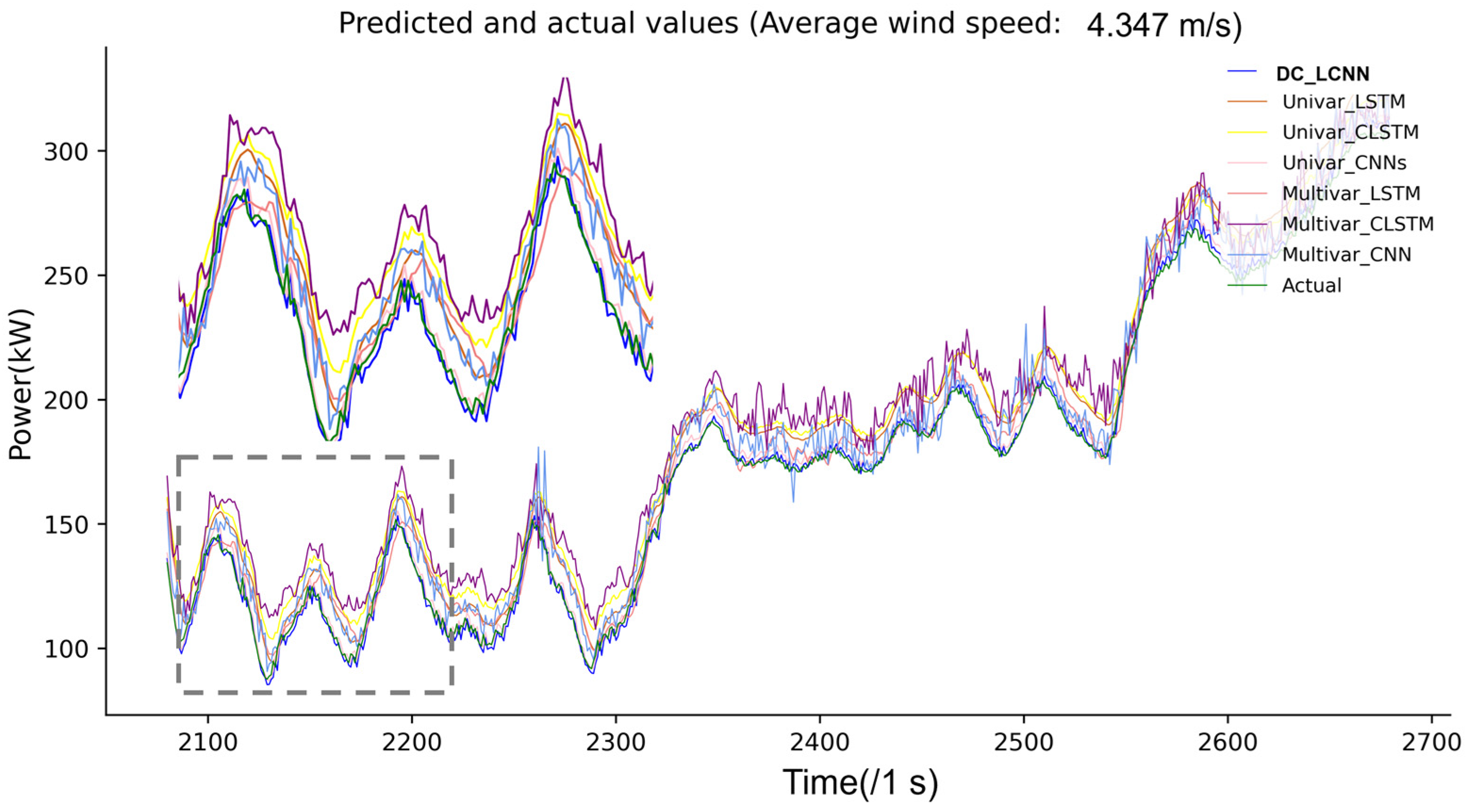
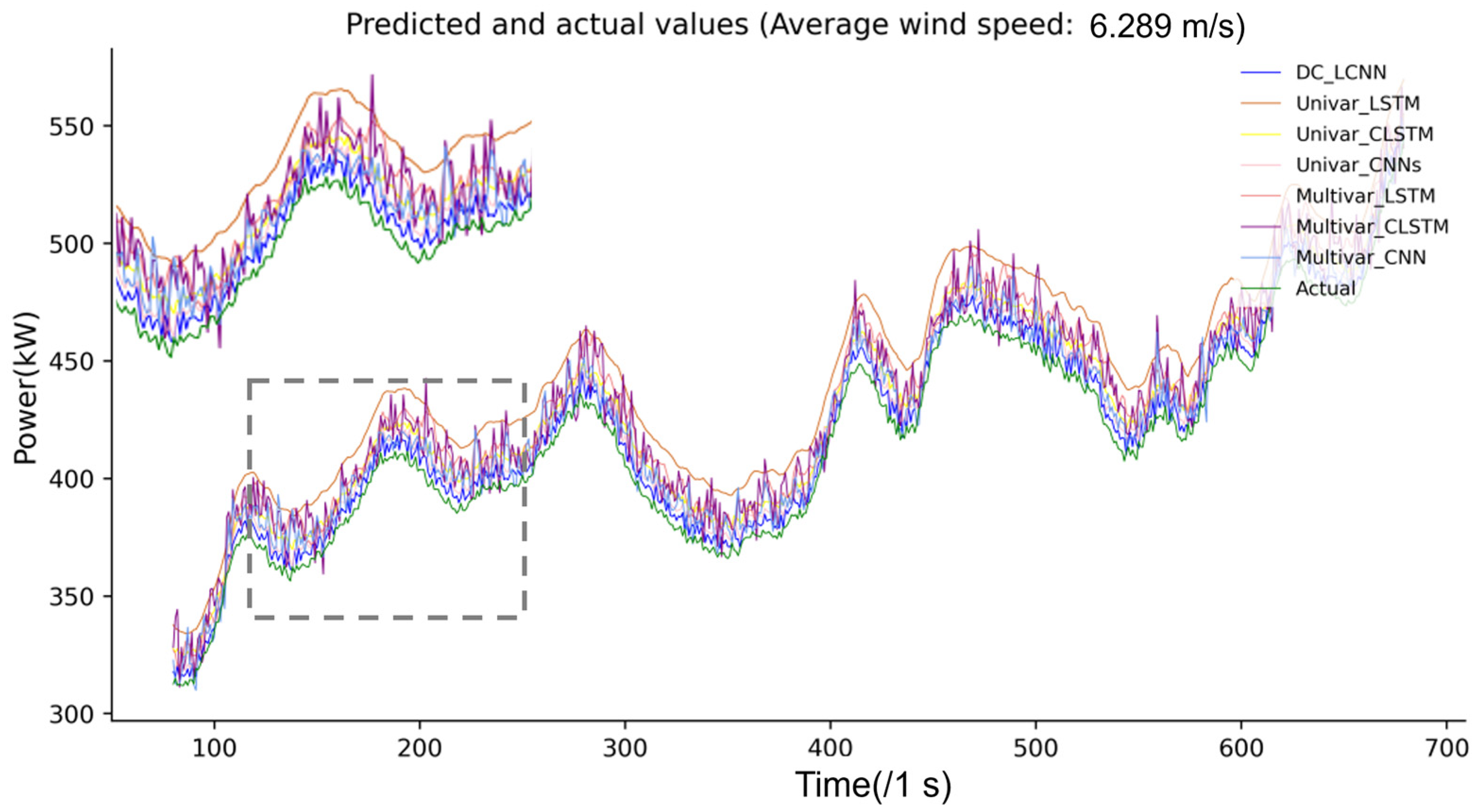
In order to demonstrate the excellent forecasting curve fitting ability of the proposed models more visually, the experiments are given as line plots of the forecasting results versus the actual values for all models for 10 consecutive minutes. In order to reflect the forecasting performance of the models at different average wind speeds, further line plots of the forecasting results at four average wind speeds are given, as shown in Figure 6, Figure 7, Figure 8 and Figure 9. For clarity of presentation, we have zoomed in locally (the dashed box part of the figure). It can be seen that the proposed model shows the best curve fitting performance on all four average wind speed intervals, where the fit is better on the lowest average wind speed (4.347 m/s) (Figure 6) and the highest average wind speed (7.347 m/s) (Figure 9) intervals. And, on the highest average wind speed interval, all models showed better fitting ability.

4.2.2. Multi-Step Second Wind Power Forecasting Task Experiments

In order to meet the application requirements of second forecasting scenarios on different time scales and to demonstrate the applicability of the proposed model architecture, multi-step wind power forecasting tasks with 1~10 s ahead of time are executed.
Channel ablation experiment for the proposed model are performed. The steps and process of this experiment are the same as the advance 1 wind power forecasting task. Multi-step forecasting of wind power from 1 to 10 s ahead is performed for each single-channel model and the proposed model, respectively, and the experimental results are shown in Table 9. Taken together, the proposed two-channel model has the optimal overall forecasting performance at ten time steps. The forecasting accuracy of all models shows an overall decreasing trend with the increase in time steps. It also proves that the proposed dual-channel structure can obtain richer and more valuable sequence feature information from the original data.
Experiments comparing the light convolutional structure of the proposed model with the traditional CNN structure replacement are conducted. The experimental procedure is the same as that of the single-step wind power prediction experiment. The two convolutional structures are used for multi-step forecasting of wind power 1~10 s ahead of time, and the experimental results are shown in Table 10. It can be seen that the forecasting results of the proposed model are still significantly better than those of the traditional CNN structure. The forecasting and training times under the two structures are shown in Table 11. It can be seen that the proposed structure has shorter forecasting and training times. In conclusion, the proposed light convolutional structure still significantly outperforms the traditional CNN structure in both forecasting accuracy and efficiency on the forecasting task of 1~10 s ahead of time.
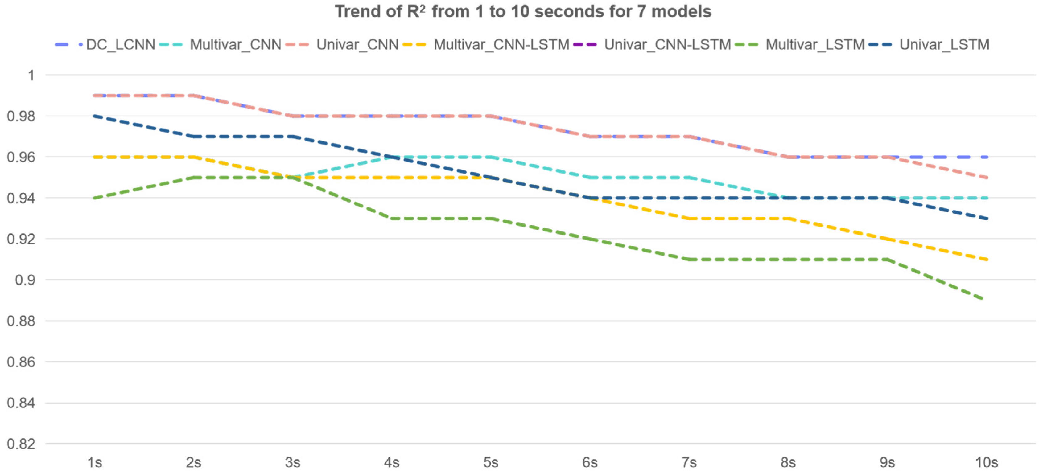
A comparison experiment with the classical deep learning baseline model is conducted. The experimental procedure is the same as the single-step wind power forecasting comparison experiment. The experimental results are shown in Table 12. Figure 10, Figure 11 and Figure 12 give the graphs of the variation in MAE, RMSE, and R2 for the seven models at time steps from 1 to 10 s, respectively. It can be seen that the forecasting accuracy and curve fitting ability of all the models show a decreasing trend with the increase in the time step. The proposed model has the highest forecasting accuracy overall, the traditional CNN with univariate input pattern achieves the second highest forecasting accuracy, and the proposed model and the traditional CNN with univariate input pattern have similar superior curve fitting abilities.
It can also be seen from Table 11 that the RE of the proposed model performs best overall. It shows that the proposed model predicts the trend of the observed series more accurately compared to the other baseline models. In the first few steps of the forecast interval, the RE of the proposed model is smaller than that of the later steps, which suggests that the model may be more advantageous for predicting the trend of sequences in shorter intervals. For the Univar_LSTM model, it has a certain advantage in forecasting the sequence trend in the later steps, which suggests that the LSTM is more advantageous for the sequence trend on the longer intervals.
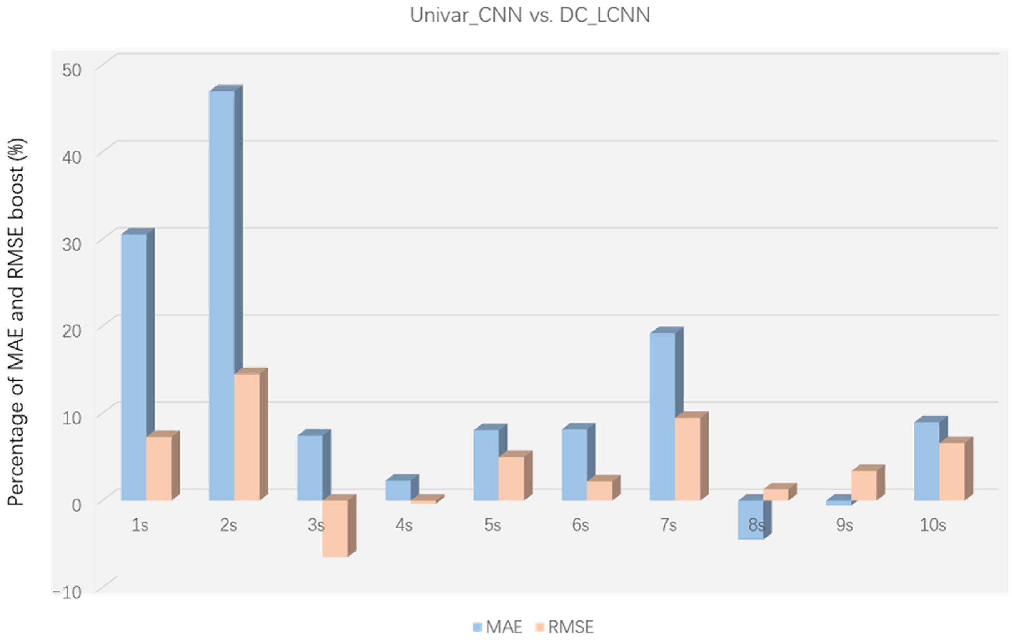
In order to further demonstrate the forecasting performance of the proposed model compared to other models, the forecasting results of the proposed model are individually compared with those of the conventional CNN model with the univariate input pattern, which has the best forecasting performance among the other models. The percentage of the boost in the MAE and RMSE of the proposed model with respect to CNN at 1 to 10 time steps is shown in Figure 13. It can be seen that the proposed model achieves better forecasting accuracy for most of the other time steps, except for the MAE of the proposed model at the eighth and ninth seconds, which is slightly inferior to the CNN, and the RMSE at the third second, which is slightly inferior to the CNN. The maximum MAE and RMSE boosts occur at time step 2, which are 46.99% and 14.53%, respectively.
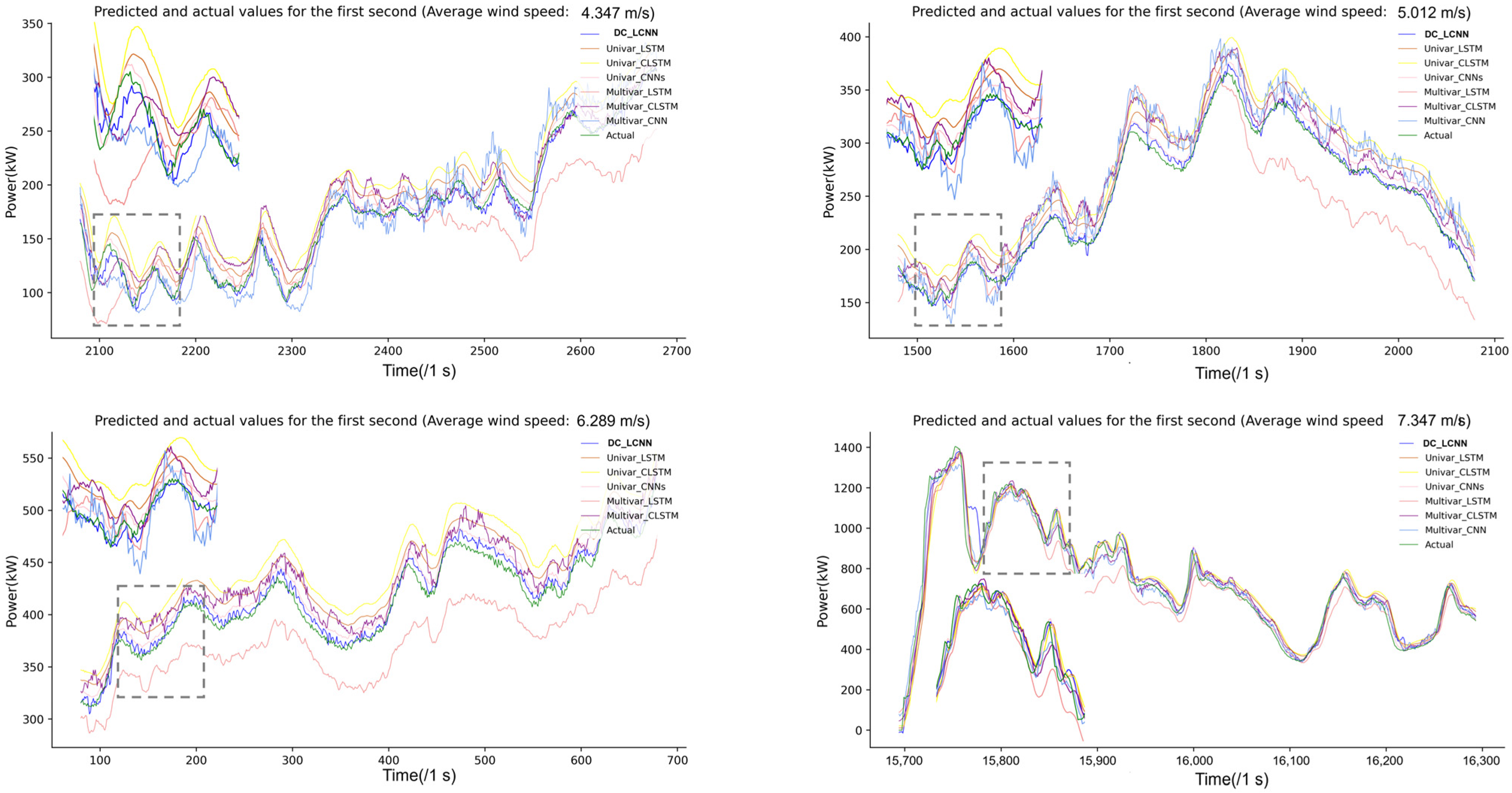
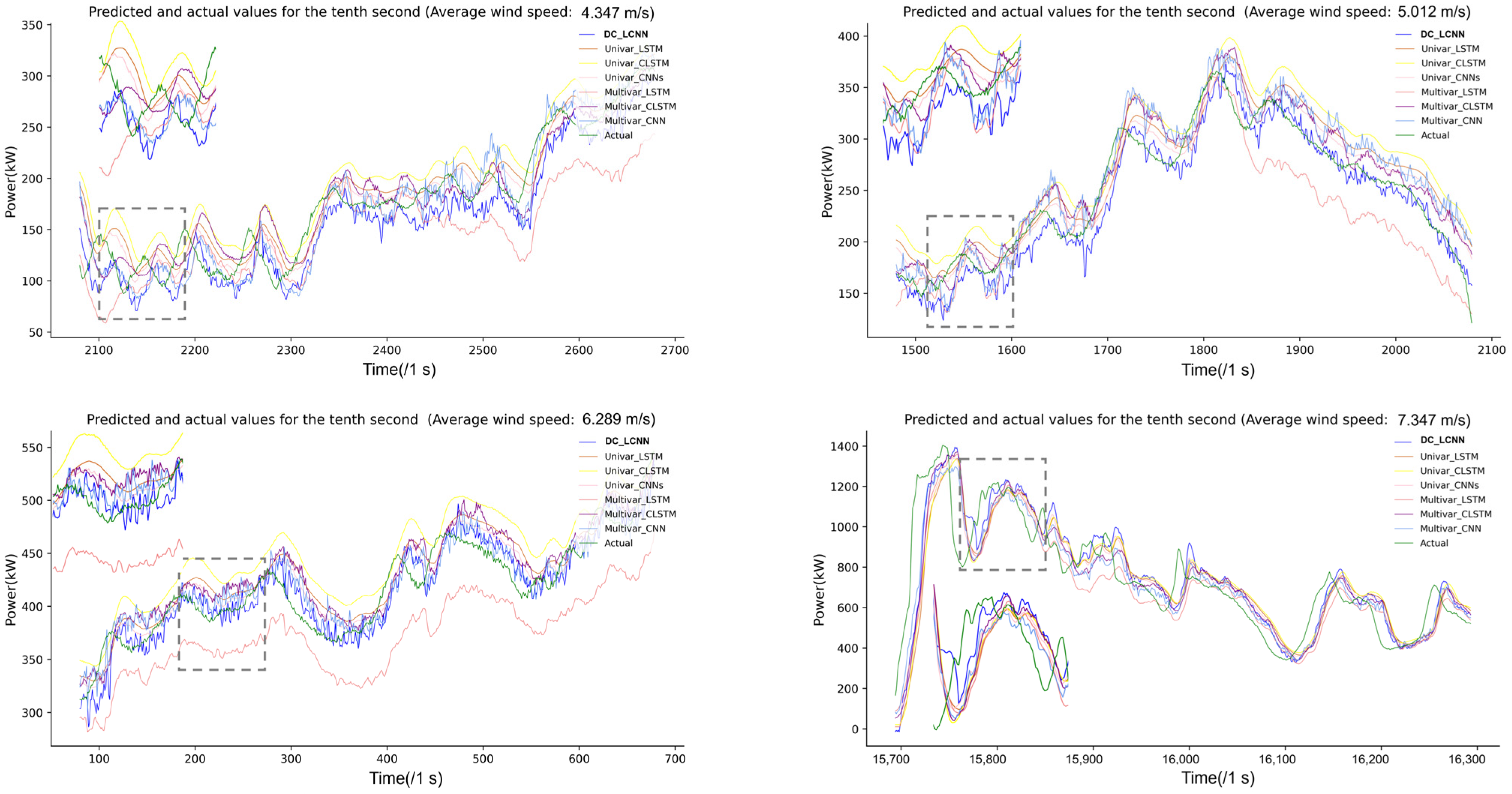
In order to demonstrate more visually and comprehensively the curve fitting ability of the proposed models at multiple forecasting time steps, the experiments are presented in the form of line plots of the predicted results versus the actual values for all the models for consecutive 10 min periods at time steps 1, 5, and 10. Similarly, to reflect the forecasting performance of the models over different average wind speed intervals, further line plots of the forecasting results at four average wind speeds are given for these three time steps, as shown in Figure 14, Figure 15 and Figure 16. For clarity of presentation, we have zoomed in locally (the dashed box part of the figure). It can be seen that on the four average wind speed intervals at time step 1, similar to the single-step forecast results, the proposed model shows the best curve fitting performance, with better fits on the lowest average wind speed (4.347 m/s) and the highest average wind speed (7.347 m/s) intervals. On the highest average wind speed interval, all models show better fitting abilities; on the four average wind speed intervals at time step 5, all models show more or less a delay in the forecast results, and the proposed model has the smallest delay and shows the best curve fitting performance, with relatively better fitting results on the lowest average wind speed (4.347 m/s) and the highest average wind speed (7.347 m/s) intervals. The fit is relatively better in the lowest average wind speed (4.347 m/s) and highest average wind speed (7.347 m/s) intervals. On the highest average wind speed interval, all models still show the best fitting ability; on the four average wind speed intervals at time step 10, the forecasts of all models show a greater degree of delay, while the proposed model has a relatively smaller degree of delay and shows the best curve fitting performance. On the highest average wind speed interval, all models still showed the best fitting ability.
In addition, from the above line graph, it can be found that as the forecasting time step increases, the delay of the forecasting results of the model with the univariate input pattern is relatively larger, in general, compared with the models with other multivariate input patterns, which indicates that the joint series of the historical power and other wind speed and direction as an input feature can provide more constraint information to the model in terms of the trend of the series changes. It also reflects the advantage of the proposed model’s two-channel input pattern.

5. Conclusions

With the large proportion of renewable energy connected to the power grid, the requirements for wind power forecasting are getting higher and higher, and the importance of high temporal resolution wind power forecasting algorithms with higher accuracy and real-time performance is also coming to the fore. In this paper, we innovatively propose a high-resolution refined wind power forecasting model based on a light convolutional neural network, DC_LCNN, which starts from the “source” data and constructs a dual-channel input model for the neural network. The model starts from the “source” data and constructs a dual-channel input mode to provide richer and more diverse feature information for the neural network; utilizes the local cross-feature extraction capability of the convolutional neural network and the computing mechanism of weight sharing and pooling to achieve an accurate and fast forecasting performance; and makes use of the global max-pooling method’s most salient feature extraction and data dimensionality reduction function to replace the FC’s weight allocation and dimension conversion function in traditional CNN to improve the model’s forecasting accuracy and efficiency.
Considering the demand of power systems for the application of high-resolution wind power prediction results on different time scales, this study performs the tasks of single-step wind power prediction with a 1 s ahead of time and multi-step wind power forecasting with a 1~10 s ahead of time. In order to demonstrate the forecasting performance of the proposed model, two groups of six experiments are carried out. The results show that the proposed method in this paper has high accuracy and real-time performance.
In conclusion, the results of this study show that the deep integration of raw data with the computing mechanism of the forecasting algorithm and the rational design of the model architecture is a proven method to improve the performance of the forecasting model. Good results are demonstrated in the task of wind power forecasting with high temporal resolution. In future work, a more in-depth and comprehensive study of deep learning-based wind power forecasting methods will be carried out on longer high-resolution datasets containing more wind conditions.

Author Contributions

Conceptualization, F.Z., Y.L. and X.R.; data curation, F.Z.; funding acquisition, F.Z. and Y.L.; methodology, Y.L., F.Z. and X.R.; software, X.R.; visualization, F.Z.; writing—original draft, F.Z. and X.R. All authors have read and agreed to the published version of the manuscript.

Funding

This research work was supported by the National Key Research and Development Program of China, No. 2019YFE0104800; Inner Mongolia Autonomous Region Key R&D and the Achievement Transformation Program Project, No. 2021GG0048.

Data Availability Statement

The data presented in this study are available on request from the corresponding author. The data are not publicly available due to be kept confidential.

Conflicts of Interest

The authors declare no conflicts of interest.

References

  1. Chandran, V.; Patil, C.K.; Manoharan, A.M.; Ghosh, A.; Sumithra, M.; Karthick, A.; Rahim, R.; Arun, K. Wind power forecasting based on time series model using deep machine learning algorithms. Mater. Today Proc. 2021, 47, 115–126. [Google Scholar] [CrossRef]
  2. Dolatabadi, A.; Jadidbonab, M.; Mohammadi-Ivatloo, B. Short-term scheduling strategy for wind-based energy hub: A hybrid stochastic/IGDT approach. IEEE Trans. Sustain. Energy 2019, 10, 438–448. [Google Scholar] [CrossRef]
  3. Hu, T.; Wu, W.; Guo, Q.; Sun, H.; Shi, L.; Shen, X. Very short-term spatial and temporal wind power forecasting: A deep learning approach. CSEE J. Power Energy Syst. 2020, 6, 434–443. [Google Scholar]
  4. Zhao, W.; Wei, Y.-M.; Su, Z. One day ahead wind speed forecasting: A resampling-based approach. Appl. Energy 2016, 178, 886–901. [Google Scholar] [CrossRef]
  5. Zhao, H.; Wu, Q.; Wang, J.; Liu, Z.; Shahidehpour, M.; Xue, Y. Combined Active and Reactive Power Control of Wind Farms based on Model Predictive Control. IEEE Trans. Energy Convers. 2017, 32, 1177–1187. [Google Scholar] [CrossRef]
  6. Gazafroudi, A.S. Assessing the impact of load and renewable energies’ uncertainty on a hybrid system. Int. J. Energy Power Eng. 2016, 5, 1–8. [Google Scholar] [CrossRef]
  7. Jung, J.; Broadwater, R.P. Current status and future advances for wind speed and power forecasting. Renew. Sustain. Energy Rev. 2014, 31, 762–777. [Google Scholar] [CrossRef]
  8. Li, Z.; Han, J.; Song, Y. On the forecasting of high-frequency financial time series based on ARIMA model improved by deep learning. J. Forecast. 2020, 39, 1081–1097. [Google Scholar] [CrossRef]
  9. Biyun, C.; Suifeng, W.; Yongjun, Z.; Ping, H. Wind power prediction model considering smoothing effects. In Proceedings of the 2013 IEEE PES Asia-Pacific Power and Energy Engineering Conference (APPEEC 2013), Kowloon, Hong Kong, 8–11 December 2013; pp. 1–4. [Google Scholar]
  10. Hu, J.; Heng, J.; Wen, J.; Zhao, W. Deterministic and probabilistic wind speed forecasting with de-noising-reconstruction strategy and quantile regression based algorithm. Renew. Energy 2020, 162, 1208–1226. [Google Scholar] [CrossRef]
  11. Ma, L.; Luan, S.; Jiang, C.; Liu, H.; Zhang, Y. A review on the forecasting of wind speed and generated power. Renew. Sustain. Energy Rev. 2009, 13, 915–920. [Google Scholar]
  12. Shi, Z.; Liang, H.; Dinavahi, V. Direct interval forecast of uncertain wind power based on recurrent neural networks. IEEE Trans. Sustain. Energy 2018, 9, 1177–1187. [Google Scholar] [CrossRef]
  13. Liu, H.; Mi, X.-W.; Li, Y.-F. Wind speed forecasting method based on deep learning strategy using empirical wavelet transform, long short term memory neural network and Elman neural network. Energy Convers. Manag. 2018, 156, 498–514. [Google Scholar] [CrossRef]
  14. Ren, X.; Zhang, F.; Zhu, H.; Liu, Y. Quad-kernel deep convolutional neural network for intra-hour photo-voltaic power forecasting. Appl. Energy 2022, 323, 119682. [Google Scholar] [CrossRef]
  15. Moharm, K.; Eltahan, M.; Elsaadany, E. Wind speed forecast using LSTM and biLSTM algorithms over gabal el-zayt wind farm. In Proceedings of the 2020 International Conference on Smart Grids and Energy Systems (SGES), Perth, Australia, 23–26 November 2020; pp. 922–927. [Google Scholar]
  16. Yu, R.; Gao, J.; Yu, M.; Lu, W.; Xu, T.; Zhao, M.; Zhang, J.; Zhang, R.; Zhang, Z. LSTM-EFG for wind power forecasting based on sequential correlation features. Future Gener. Comput. Syst. 2019, 93, 33–42. [Google Scholar] [CrossRef]
  17. Xin, Z.; Liu, X.; Zhang, H.; Wang, Q.; An, Z.; Liu, H. An enhanced feature extraction based long short-term memory neural network for wind power forecasting via considering the missing data reconstruction. Energy Rep. 2024, 11, 97–114. [Google Scholar] [CrossRef]
  18. Sun, Y.; He, J.; Ma, H.; Yang, X.; Xiong, Z.; Zhu, X.; Wang, Y. Online chatter detection considering beat effect based on Inception and LSTM neural networks. Mech. Syst. Signal Process. 2023, 184, 109723. [Google Scholar] [CrossRef]
  19. Yang, T.; Li, B.; Xun, Q. LSTM-attention-embedding model-based day-ahead prediction of photovoltaic power output using Bayesian optimization. IEEE Access 2019, 7, 171471–171484. [Google Scholar] [CrossRef]
  20. Shu, X.; Zhang, L.; Sun, Y.; Tang, J. Host–parasite: Graph LSTM-in-LSTM for group activity recognition. IEEE Trans. Neural Netw. Learn. Syst. 2021, 32, 663–674. [Google Scholar] [CrossRef]
  21. Wang, H.-Z.; Li, G.-Q.; Wang, G.-B.; Peng, J.-C.; Jiang, H.; Liu, Y.-T. Deep learning based ensemble approach for probabilistic wind power forecasting. Appl. Energy 2017, 188, 56–70. [Google Scholar] [CrossRef]
  22. Acikgoz, H.; Budak, U.; Korkmaz, D.; Yildiz, C. WSFNet: An efficient wind speed forecasting model using channel attention-based densely connected convolutional neural network. Energy 2021, 233, 121121. [Google Scholar] [CrossRef]
  23. Houran, M.A.; Bukhari, S.M.S.; Zafar, M.H.; Mansoor, M.; Chen, W. COA-CNN-LSTM: Coati optimization algorithm-based hybrid deep learning model for PV/wind power forecasting in smart grid applications. Appl. Energy 2023, 349, 121638. [Google Scholar] [CrossRef]
  24. Nguyen, T.H.T.; Phan, Q.B. Hourly day ahead wind speed forecasting based on a hybrid model of EEMD, CNN-Bi-LSTM embedded with GA optimization. Energy Rep. 2022, 8, 53–60. [Google Scholar] [CrossRef]
  25. Li, N.; Dong, J.; Liu, L.; Li, H.; Yan, J. A novel EMD and causal convolutional network integrated with Transformer for ultra short-term wind power forecasting. Int. J. Electr. Power Energy Syst. 2023, 154, 109470. [Google Scholar] [CrossRef]
  26. Yuan, P.; Jiao, Y.; Li, J.; Xia, Y. A densely connected causal convolutional network separating past and future data for filling missing PM2.5 time series data. Heliyon 2024, 10, e24738. [Google Scholar] [CrossRef] [PubMed]
  27. Sun, S.; Liu, Y.; Li, Q.; Wang, T.; Chu, F. Short-term multi-step wind power forecasting based on spatio-temporal correlations and transformer neural networks. Energy Convers. Manag. 2023, 283, 116916. [Google Scholar] [CrossRef]
  28. Zhu, J.; Su, L.; Li, Y. Wind power forecasting based on new hybrid model with TCN residual modification. Energy AI 2022, 10, 100199. [Google Scholar] [CrossRef]
  29. Gong, M.; Yan, C.; Xu, W.; Zhao, Z.; Li, W.; Liu, Y.; Li, S. Short-term wind power forecasting model based on temporal convolutional network and Informer. Energy 2023, 283, 129171. [Google Scholar] [CrossRef]
  30. Islam, M.; Barua, P.; Rahman, M.; Ahammed, T.; Akter, L.; Uddin, J. Transfer learning architectures with fine-tuning for brain tumor classification using magnetic resonance imaging. Healthc. Anal. 2023, 4, 100270. [Google Scholar] [CrossRef]
  31. Mirza, A.F.; Mansoor, M.; Usman, M.; Ling, Q. Hybrid Inception-embedded deep neural network ResNet for short and medium-term PV-Wind forecasting. Energy Convers. Manag. 2023, 294, 117574. [Google Scholar] [CrossRef]
  32. Zhang, F.; Li, P.C.; Gao, L.; Liu, Y.Q.; Ren, X.Y. Application of autoregressive dynamic adaptive (ARDA) model in real-time wind power forecasting. Renew. Energy 2021, 169, 129–143. [Google Scholar] [CrossRef]
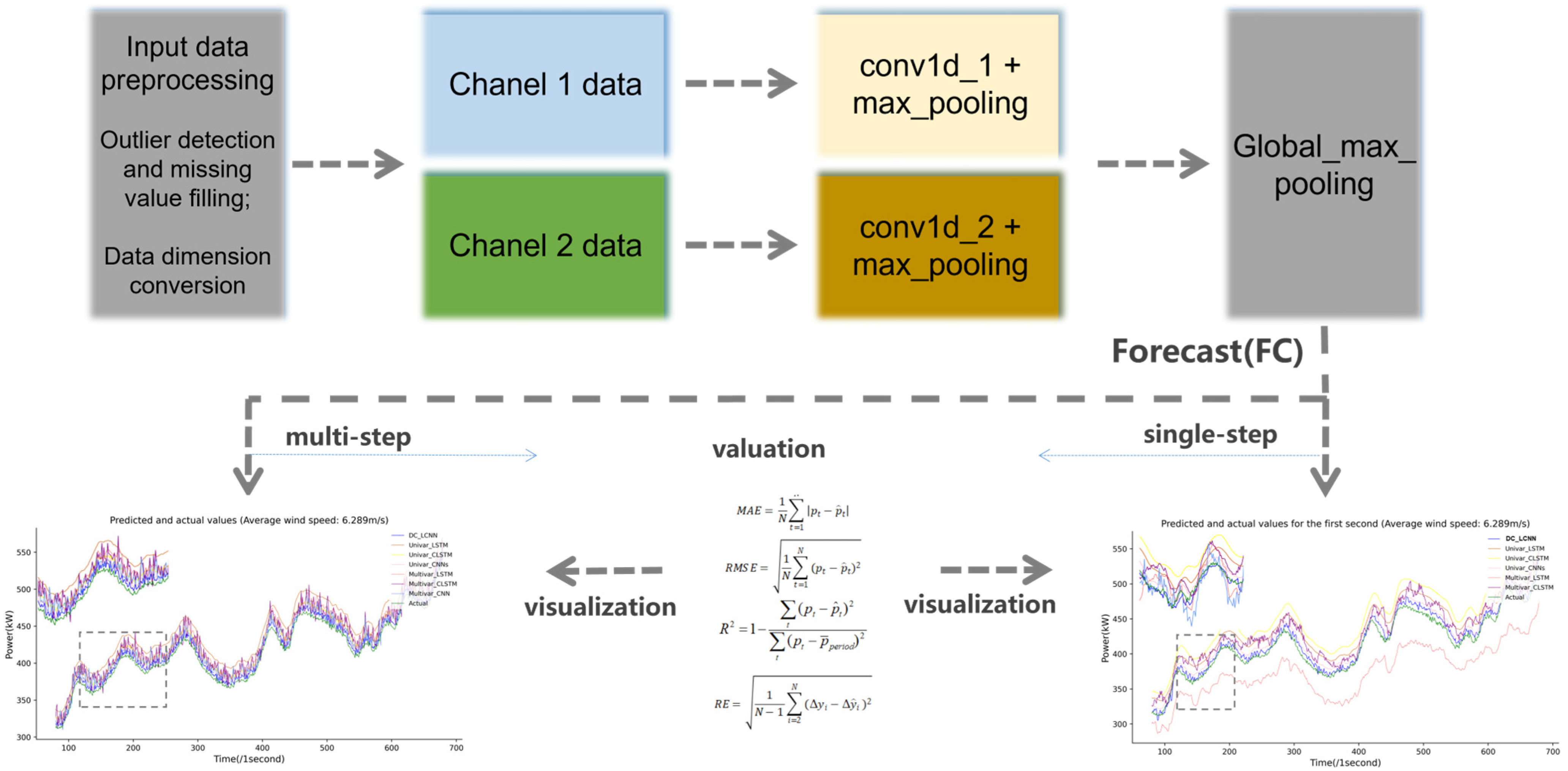
Figure 1. The overall research flow of the methodology proposed.
Energies 17 01183 g001
Figure 2. The architecture of the proposed model.
Energies 17 01183 g002
Figure 3. Changes in each variable over time.
Energies 17 01183 g003
Figure 4. Comparison of persistence model and proposed model forecasting results on larger wind power fluctuation intervals. (a,b) show line plots of the proposed model and the persistence model against the measured values, respectively; (c,d) show enlargements of the rectangular dashed box areas in (a,b), respectively.
Energies 17 01183 g004
Figure 5. Percentage boost in MAE and RMSE of the proposed model compared to the baseline models.
Energies 17 01183 g005
Figure 6. Predicted and actual values of seven models with 1 s ahead of time on the 4.347 m/s average wind speed interval.
Energies 17 01183 g006
Figure 7. Predicted and actual values of seven models with 1 s ahead of time on the 5.012 m/s average wind speed interval.
Energies 17 01183 g007
Figure 8. Predicted and actual values of seven models with 1 s ahead of time on the 6.289 m/s average wind speed interval.
Energies 17 01183 g008
Figure 9. Predicted and actual values of seven models with 1 s ahead of time on the 7.347 m/s average wind speed interval.
Energies 17 01183 g009
Figure 10. Trend of MAE from 1 to 10 s for seven models.
Energies 17 01183 g010
Figure 11. Trend of RMSE from 1 to 10 s for seven models.
Energies 17 01183 g011
Figure 12. Trend of R2 from 1 to 10 s for seven models.
Energies 17 01183 g012
Figure 13. Percentage boost in MAE and RMSE of the proposed model compared to the univariate input pattern CNN model.
Energies 17 01183 g013
Figure 14. Predicted and actual values of wind power at the first second for seven models on four average wind speed intervals.
Energies 17 01183 g014
Figure 15. Predicted and actual values of wind power at the fifth second for seven models on four average wind speed intervals.
Energies 17 01183 g015
Figure 16. Predicted and actual values of wind power at the tenth second for seven models on four average wind speed intervals.
Energies 17 01183 g016
Table 1. The parameters of the proposed model.
The Layers for DC_LCNNParameters of Each Layer
Conv1D_1(Input 1)Filters = 32, kernel size = 2, stride = 1, activation = ‘relu’, padding = ‘same’
MaxPooling1D_1Kernel size = 2, stride = 1
Conv1D_2(Input 2)Filters = 32, kernel size = 2, stride = 1, activation = ‘relu’, padding = ‘same’
MaxPooling1D_2Kernel size = 2, stride = 1
Dropout_2Rate = 0.1
Conv1D_3Filters = 32 (single-step forecasting), filters = 10 (multi-step forecasting), kernel size = 2, stride = 1, activation = ‘relu’, padding = ‘same’
Global_MaxPooling1D_1-
DenseNeurons = 1 (single-step forecasting); neurons = 10 (multi-step forecasting)
Others Epoches = 150; EarlyStopping:monitor = ‘mse’; batch size = 24, patience = 5; min_delta = 0.0001
Table 2. The parameters of the baseline models.
ModelsThe Layers Parameters of Each Layer
Univar_LSTM
and
Multivar_LSTM
LSTMNeurons = 32 (single-step forecasting); neurons = 20 (multi-step forecasting); activation = ‘relu’; return_sequences = True
Flatten-
DenseNeurons = 128 (single-step forecasting); neurons = 400 (multi-step forecasting); activation = ‘relu’; kernel_regularizer = l2 (0.0001)
DenseNeurons = 1 (single-step forecasting); neurons = 10 (multi-step forecasting)
Univar_CNN-LSTM
and
Multivar_CNN-LSTM
Conv1DFilters = 32; kernel size = 2; stride = 1; activation = ‘relu; padding = ‘same’
MaxPooling1DKernel size = 2; stride = 1
LSTMNeurons = 128 (single-step forecasting); neurons = 320 (multi-step forecasting); activation = ‘relu’; return_sequences = True
Flatten-
DenseNeurons = 128 (single-step forecasting); neurons = 320 (multi-step forecasting); activation = ‘relu’; kernel_regularizer = l2 (0.0001)
DenseNeurons = 1 (single-step forecasting); neurons = 10 (multi-step forecasting)
Univar_CNNConv1D_1Filters = 32; kernel size = 2; stride = 1; activation = ‘relu’; padding = ‘same’
MaxPooling1D_1Kernel size = 2; stride = 1
Conv1D_2Filters = 32; kernel size = 2; stride = 1; activation = ‘relu’; padding = ‘same’
MaxPooling1D_2kernel size = 2; stride = 1
Flatten-
DenseNeurons = 64 (single-step forecasting); neurons = 160 (multi-step forecasting); activation = ‘relu’; kernel_regularizer = l2 (0.0001)
DenseNeurons = 1 (single-step forecasting); neurons = 10 (multi-step forecasting)
Multivar_CNNConv1D_1Filters = 32; kernel size = 2; stride = 1; activation = ‘relu’; padding = ‘same’
MaxPooling1D_1Kernel size = 2; stride = 1
Conv1D_2Filters = 32; kernel size = 2; stride = 1; activation = ‘relu’; padding = ‘same’
MaxPooling1D_2Kernel size = 2; stride = 1
Flatten-
DropoutRate = 0.1
DenseNeurons = 64 (single-step forecasting); neurons = 160 (multi-step forecasting); activation = ‘relu’; kernel_regularizer = l2 (0.0001)
DenseNeurons = 1 (single-step forecasting); neurons = 10 (multi-step forecasting)
Other public parametersEpoches = 150; EarlyStopping:monitor = ‘mse’; batch size = 120 (single-stepforecasting); batch size = 120 (multi-stepforecasting); patience = 5; min_delta = 0.0001
Table 3. The forecasting results comparison of the ablation experiments of single-step forecasting.
ModelMAE (kW)RMSE (kW)R2
DC1_LCNN 8.9599.7791
DC2_LCNN13.86219.2330.98
DC_LCNN4.6256.0611
The bold in the first column of the table represents the model proposed in this paper. The bold numbers in the table represent the best forecasts at the corresponding index. Bolded text in subsequent tables conveys the same meaning as in this table.
Table 4. Comparison of the forecast results of the light convolutional structure of the proposed model with the traditional CNN structure in single-step forecasting.
ModelMAE (kW)RMSE (kW)R2
DC_CNN (FC) 8.9599.7791
DC_LCNN4.6256.0611
The bold in the first column of the table represents the model proposed in this paper. The bold numbers in the table represent the best forecasts at the corresponding index. Bolded text in subsequent tables conveys the same meaning as in this table.
Table 5. Running time comparison of the proposed model’s light convolutional structure with the conventional CNN structure experiment in single-step forecasting.
ModelTraining Time (s)Forecast Time (s)Forecast Time for Each Step (s)
DC_CNN (FC) 161.7681.2351.235/17,280
DC_LCNN80.6960.9160.916/17,280
The bold in the first column of the table represents the model proposed in this paper. The bold numbers in the table represent the best forecasts at the corresponding index. Bolded text in subsequent tables conveys the same meaning as in this table.
Table 6. Comparison of the performance of the persistence model and the proposed model.
ModelMAE (kW)RMSE (kW)Maximum Absolute Error (kW)
Persistence 3.2585.920153.60
DC_LCNN4.6256.06186.32
The bold in the first column of the table represents the model proposed in this paper. The bold numbers in the table represent the best forecasts at the corresponding index. Bolded text in subsequent tables conveys the same meaning as in this table.
Table 7. Comparison of the performance of the persistence model and the proposed model with large changes in wind power.
ModelMAE (kW)
(Figure 4a,b)
RMSE (kW)
(Figure 4a,b)
MAE (kW)
(Figure 4c,d)
RMSE (kW)
(Figure 4c,d)
Persistence 13.3220.9166.3688.48
DC_LCNN10.1614.1749.1762.27
The bold in the first column of the table represents the model proposed in this paper. The bold numbers in the table represent the best forecasts at the corresponding index.
Table 8. Comparison of seven model forecast results for sigle-step forecasting in single-step forecasting.
IndexesUnivar_LSTMMultivar_LSTMUnivar_CNN-LSTMMultivar_CNN-LSTMUnivar_CNNMultivar_CNNDC_LCNN
MAE22.9915.4014.2317.117.77611.574.625
RMSE24.8117.8614.8919.278.9717.496.06
R20.980.990.990.991.00.991.0
RE4.524.894.6210.244.917.844.47
The bold numbers in the table represent the best forecasts at the corresponding index.
Table 9. The forecasting results comparison of the ablation experiments of multi-step forecasting.
ModelsIndexesTime Steps (s)
12345678910
DC1_LCNNMAE9.02310.6612.1213.8219.4413.7715.9118.8620.8420.52
RMSE14.2718.4021.3021.8630.8228.3429.9134.9538.5038.90
R20.990.990.980.980.970.970.970.950.950.93
DC2_LCNNMAE21.9226.3827.7121.8435.6539.3640.7735.4334.9235.68
RMSE31.1539.1839.6237.2449.5648.9349.8249.9449.1250.73
R20.960.950.950.950.920.920.910.920.920.91
DC_LCNNMAE7.3117.61713.6513.6912.2916.2914.3018.9419.3419.62
RMSE11.6814.8821.2121.5722.4327.5927.4532.6833.5935.83
R20.990.990.980.980.980.970.970.960.960.96
The bold in the first column of the table represents the model proposed in this paper. The bold numbers in the table represent the best forecasts at the corresponding time step.
Table 10. Comparison of the forecast results of the light convolutional structure of the proposed model with the traditional CNN structure in multi-step forecasting.
ModelsIndexesTime Steps (s)
12345678910
DC_LCNN (FC)MAE30.2015.5424.5023.4629.0922.3832.7726.1035.4431.88
RMSE31.9521.7728.7829.5735.2231.8840.9738.0445.8445.09
R20.970.980.970.970.960.970.940.950.930.93
DC_LCNNMAE7.3117.61713.6513.6912.2916.2914.3018.9419.3419.62
RMSE11.6814.8821.2121.5722.4327.5927.4532.6833.5935.83
R20.990.990.980.980.980.970.970.960.960.96
The bold in the first column of the table represents the model proposed in this paper. The bold numbers in the table represent the best forecasts at the corresponding time step.
Table 11. Running time comparison of the proposed model’s light convolutional structure with the conventional CNN structure experiment in multi-step forecasting.
ModelTraining Time (s)Forecast Time (s)Forecast Time for Each Step (s)
DC_CNN (FC) 246.4781.4201.420/17,280
DC_LCNN158.9230.9810.981/17,280
The bold in the first column of the table represents the model proposed in this paper. The bold numbers in the table represent the best forecasts for the corresponding term.
Table 12. Comparison of seven model forecast results in multi-step forecasting.
ModelsIndexesTime Steps (s)
12345678910
Univar_LSTMMAE22.0422.7623.6623.8423.4525.5625.3125.9026.9926.99
RMSE25.6828.1630.5532.4934.0737.3538.8541.1243.5444.89
R20.980.970.970.960.950.940.940.940.940.93
RE4.414.734.965.115.205.285.365.405.435.47
Multivar_LSTMMAE33.8730.1330.3535.0432.4634.7136.0236.5234.6539.35
RMSE43.3538.6139.7046.7343.9947.9850.4352.0150.2356.54
R20.940.950.950.930.930.920.910.910.910.89
RE4.945.295.485.555.625.695.745.85.85.87
Univar_CNN-
LSTM
MAE32.2531.1333.0232.5332.6532.8735.3234.8734.0337.87
RMSE34.9735.1637.9339.0440.0742.3545.3846.7447.7951.67
R20.960.960.950.950.940.940.930.930.920.91
RE4.494.744.945.135.195.375.385.405.465.52
Multivar_CNN-LSTMMAE18.9419.0317.7120.7621.0121.1122.9922.9323.5526.19
RMSE24.7726.2126.6730.0631.8433.6636.6537.8540.4043.30
R20.980.980.980.970.970.960.950.950.940.94
RE6.176.376.546.626.586.586.476.576.456.49
Univar_CNNMAE10.5314.3714.7513.9713.3717.7417.7018.0819.2321.56
RMSE12.6017.4119.8321.6523.6228.2030.3333.1134.7838.36
R20.990.990.980.980.980.970.970.960.960.95
RE4.224.645.105.275.305.405.495.495.645.68
Multivar_CNNMAE22.4622.2425.0021.9222.7423.8424.8428.5127.7026.88
RMSE33.1432.7836.5734.3634.5737.2639.0642.2442.8043.51
R20.960.960.950.960.960.950.950.940.940.94
RE9.8710.0910.2910.1910.1210.4010.339.899.909.80
DC_LCNNMAE7.3117.61713.6513.6912.2916.2914.3018.9419.3419.62
RMSE11.6814.8821.2121.5722.4327.5927.4532.6833.5935.83
R20.990.990.980.980.980.970.970.960.960.96
RE4.134.594.965.055.206.255.215.395.755.74
The bold in the first column of the table represents the model proposed in this paper. The bold numbers in the table represent the best forecasts at the corresponding time step.
Disclaimer/Publisher’s Note: The statements, opinions and data contained in all publications are solely those of the individual author(s) and contributor(s) and not of MDPI and/or the editor(s). MDPI and/or the editor(s) disclaim responsibility for any injury to people or property resulting from any ideas, methods, instructions or products referred to in the content.