Electromechanical Energy-Based 3D-Controllable Motion of Small Matter toward Tiny Machines

Abstract

Is it possible to remotely operate a tiny piece of matter or a less-than-one-centimeter machine to perform a medical task in life? Especially given that in the present technology, neither the mechanism nor battery is small enough to be set up inside the structure of such a tiny machine. Yet, if the powered matter is magnetically responsive, then a magnetic field, as one of the potential power sources, can be applied to power it promisingly. Herein, the concept of electromechanical energy conversion is utilized through a specific configuration consisting of eight solenoids arranged together as a nest. The device converts electrical energy into an electromagnetic field, and finally, into mechanical energy, respectively, resulting in magnetic manipulation. Since electric energy is supplied to the configuration, eight solenoids generate the controllable magnetic field in both direction and magnitude by means of the superposition technique. The device can magnetically navigate tiny motorless matter to release mechanical energy through the 3D-controllable motion to arbitrary positions effectively and physical interactions with the surrounding environment as if operating a tiny machine. The experimental results report the feasibility of the device to control the 6-DOF locomotion of small matter precisely. The contribution of the concept based on this work leads to a promising protocol to remotely power small machines, micro-engines, micro-propellers, micro-turbines, etc.

1. Introduction

Electromechanical energy conversion is the conversion of mechanical energy into electrical energy or vice versa. A device that converts electrical energy into mechanical energy or mechanical energy into electrical energy is known as an electromechanical energy conversion device. Its energy conversion takes place through the medium of a magnetic field. The magnetic field is used as a coupling medium between electrical and mechanical systems, as depicted in Figure 1. When the electromechanical energy conversion takes place from electrical energy to mechanical energy, the device is known as a motor. Whereas, when the conversion takes place from mechanical energy to electrical energy, the device is known as a generator.

In electrical machines, the conversion of energy from electrical to mechanical or from mechanical to electrical results in two electromagnetic phenomena. Firstly, when a conductor moves in a magnetic field, an electromotive force or EMF is induced in the conductor. Secondly, when a current-carrying conductor is placed in a magnetic field, a mechanical force acts on the conductor. These two effects occur simultaneously whenever energy conversion takes place from electrical to mechanical, or vice versa [1].

In addition, a multi-turn wire-carrying electric current is called an electromagnetic coil, solenoid, etc., and can produce an electromagnetic field perpendicular to the flow direction of the current [2]. Its magnetic fields are current-dependent. This concept is applied as an actuator to convert electrical energy into mechanical energy. An example is a magnetic door lock, where a solenoid exerts a magnetic force along its axial axis to a moving rod for locking.

Basically, magnetic force, wrench force, or heading force is a product of a gradient magnetic field. The Maxwell circular coil is a popular electromagnet presented in the form of a coil pair. It generates a magnetic field gradient that is almost uniform, with the direction parallel to the coaxial axis of the coil pair at the center. Two coils are coaxially arranged to have a space between them that is about the square root of three times the coil radius ($\sqrt{3r}$).

Another popular and commonly used type of electromagnet is the Helmholtz coil. It consists of two circular coils that are coaxially arranged. It provides a space between the pair equal to the radius of the coil. It is capable of generating a nearly uniform magnetic field, which produces magnetic torque. The homogeneity in the magnetic field varies depending on the demands of the application. However, further advances have been made by orthogonally arranging three pairs of Helmholtz coils, known as a triaxial Helmholtz coil, in order to generate a uniform magnetic field in an arbitrary orientation [3,4,5,6]. The outcome would be a variety of magnetic fields that exert continuous torque, such as rotating, oscillating, alternating, and conical magnetic fields.

As mentioned, the Helmholtz coil is adept in torque generation, and the Maxwell coil can exert magnetic force. Several works have combined both coil types together in order to generate plenty of force and torque in various directions, but it comes with complex arrangements. Some studies had to install a motoring unit to rotate or move coils in order to produce the desired magnetic field. For example, a triaxial Helmholtz coil was mounted outside with two Maxwell coils. This configuration relied on the change in the direction of the two Maxwell coils to exert force in a different direction [7].

There are several applications that modified both Helmholtz coils and Maxwell coils into a square shape [8], called a saddle coil. The name saddle refers to the fact that a square coil is bent into a shape similar to a saddle. It consisted of two symmetric saddle-shaped coils coaxially arranged at a specific distance. It could produce both a nearly uniform magnetic field to exert torque and a nearly gradient magnetic field to exert force, depending on the coil configuration [9]. The idea to mix both types of saddle coil was proposed in order to fulfill both torque and force generation within only one configuration [10].

Moreover, electromagnetic configurations were also proposed in the form of core-inserted electromagnetic coils with the purpose of force generation, which further added to the complexity of magnetic field distribution. Researchers then adopted direct dipole approximation to map the current field to address the difficulty of magnetic field generation. This type of electromagnet was mostly regulated to have a sufficient force in three-dimensional space and maximized force for specific medical applications (e.g., navigation of medical catheters, and ophthalmic intervention robots) [11]. Another study designed the formation of nine electromagnets that were optimized to strengthen the magnetic field gradient toward the planar direction, but they lacked a stable magnetic levitation [12]. Some works arranged electromagnets at each vertex of a cube in order to have independent control of magnetic force in all major directions [13]. Obviously, many works were constructed to meet their own demands, which could not guarantee the best configuration because a trade-off exists among force generation, torque generation, workspace, etc. However, there was rigorous quantification of the required number of electromagnets to eliminate singularity issues under different circumstances [14].

Electromechanical devices are also available as a system for commercials with costs. The active Locomotive Intestinal Capsule Endoscope (ALICE) system comprises five coil pairs: one uniform saddle coil and four coil pairs [15]. The magnetically guided capsule endoscopy (MGCE) system consists of twelve coils that are paired [16]. Some coil pairs generate both magnetic field and field gradient components, whereas others create either a magnetic field or field gradient component. The magnetic resonance imaging (MRI) scanner is a medical imaging device that uses a magnetic field. It was promisingly applied for dynamic magnetic force and one static direction of a uniform magnetic field [17,18].

Many studies in the literature configured and presented electromechanical devices to generate remote magnetic fields and further use for control objects. Presently, one of the major obstacles to building a tiny machine is that there is no current technology to fabricate a small battery and mechanism to set up inside the structure of the machine. The contribution of such a machine would be useful, especially in the field of biomedicines, biosensors, bioactuators, etc., which are operated to perform tasks inside life. Here, in this work, an electromechanical energy conversion configuration consisting of eight permalloy core-inserted solenoids is invented to serve as a solution to this problem. This is the first time that this design is considered to eliminate losses according to the theory of electromechanical energy conversion in order to improve performance and obtain rule-obeyed hardware. The configuration is also integrated with a non-complex control algorithm to generate the controllable magnetic field to remotely and wirelessly power a tiny piece of matter precisely for effective 3D locomotion. The benefit provided by this work is that the results lead to a powerful method that can remotely and wirelessly supply energy to tiny pieces of matter to fulfill applications in life promisingly [19,20].

The conceptual design and numerical simulation model are detailed in the next section. Then, the system implementation and a demonstration using the 3D-controllable motion of two types of small matter are presented to show the feasibility and performance of the proposed system. Finally, the conclusion is presented.

2. Materials and Methods

2.1. Conceptual Design

Basically, a magnetic field is a field of magnetic vectors consisting of both magnitude and direction components. The major direction of magnetic devices (e.g., permanent magnet, coil, etc.) is defined by the direction in which most magnetic vectors point toward. For example, a bar magnet has N and S poles because most magnetic vectors point to the N pole. As mentioned, the magnetic field behaves as a vector field, so two or more magnetic fields can couple, decouple, or superpose to finalize a resultant magnetic field. In order to achieve the overall direction of the magnetic field within three-dimensional space, a number of magnetic sources are arranged together as a nest, called the configuration of electromagnetic coils. The configuration as an electromechanical energy conversion device is designed to have eight solenoids, which are grouped into two sets: the upper and lower set, as depicted in Figure 2. The number of solenoids is chosen as “eight” in order to support the three-dimensional magnetic field and for coupling to avoid the singularity of the magnetic field while generating pure torque without the interference of wrench force via the dynamic magnetic field. The proposed configuration consists of two sets. The upper set consists of four solenoids arranged at the corner of a square, which are declined at 45 degrees. The lower set also consists of four solenoids arranged at the different corners of another square, which are declined at 60 degrees, as shown in Figure 2 on the left. Basically, one single solenoid generates a magnetic field along its axial axis, but because the eight solenoids are pointed to a common center, by means of the superposition technique, the setup can generate a controllable and adjustable magnetic field in both direction and magnitude upon demand perfectly. That magnetic field can manipulate a piece of matter to move to all positions across the three-dimensional space, called a region of interest (ROI) provided by the arrangement of those solenoids. Additionally, the magnetic field can still control or trigger alternative functions and physical actions of the matter (e.g., fold and unfold a component of a small mechanic body). However, the precision of the matter’s motion might not be easily achieved if losses from the conversion are not compromised. Methods to cope with this issue will be described in the next section on system implementation.

2.2. Theoretical Concept of Electromechanical Energy Conversion into Mechanical Force and Torque

According to the first law of thermodynamics, which is equivalent to the law of energy conservation: “energy cannot be created or destroyed, so the total amount of energy in the Universe is fixed.” That is, energy can be transformed from one form to another or transferred from one place to another, but the total energy must remain unchanged. Thus, electromagnetic energy conversion can be expressed by

Total electrical input = Total mechanical output + Total energy stored + Total energy dissipated

where total energy stored consists of energy stored in the coupling field and energy stored in mechanical system. Total energy dissipated consists of ohmic losses (I²R), losses in the magnetic core (e.g., hysteresis loss, eddy current loss), and losses in the mechanical system due to movement (e.g., friction, windage, fluidic loss).

Because electromechanical energy conversion uses a magnetic field as a medium to transfer mechanical energy, mathematical models of magnetic field generation adopt the Biot–Savart law [6]. Since electric current passes through a solenoid, the magnetic flux, ${\overrightarrow{\mathit{B}}}_{\mathit{p}}$, (unit: T) at a point p located away from the solenoid is expressed by

$${\overrightarrow{\mathit{B}}}_{\mathit{p}}=\frac{\mathit{I}{\mu }_0}{4\pi }{\int }_{wire}\frac{d\mathit{l}\times \overrightarrow{\mathit{r}}}{{\mathit{r}}^2}$$

(1)

where $\mathit{I}, d\mathit{l}, \overrightarrow{\mathit{r}}, r, { \mathrm{a}\mathrm{n}\mathrm{d} \mu }_0$ are the electric current flowing in a wire, the segment of the current loop, the unit vector distance, the distance from a solenoid to point p, and the permeability, $4\pi \times {10}^{-7}$ T·m/A, respectively. The magnetic field generated by the system can be expressed as a function of passing current and the field in each component x, y, and z, which is

$${\overrightarrow{\mathit{B}}}_{\mathit{p}}={\left[\begin{array}{ccc}{B}_x& B_y& B_z\end{array}\right]}^T\mathit{I}$$

(2)

A small piece of matter will receive electromechanical energy if it is magnetic-responsive. Thus, under a magnetic field, ${\overrightarrow{\mathit{B}}}_{\mathit{p}}$, matter with the magnetic moment $\stackrel{⃑}{\mathit{m}}=\left[\begin{array}{ccc}{m}_x& m_y& m_z\end{array}\right]$, (unit: A·m²), which locates at point p experiences magnetic torque, ${\overrightarrow{\mathit{T}}}_{\mathit{p}}=\left[\begin{array}{ccc}{T}_x& T_y& T_z\end{array}\right]$, (unit: N·m), and force, ${\overrightarrow{\mathit{F}}}_{\mathit{p}}=\left[\begin{array}{ccc}{F}_x& F_y& F_z\end{array}\right]$, (unit: N), which are expressed by

$${\overrightarrow{\mathit{T}}}_{\mathit{p}}=\stackrel{⃑}{\mathit{m}}\times {\overrightarrow{\mathit{B}}}_{\mathit{p}}$$

(3)

$${\overrightarrow{\mathit{F}}}_{\mathit{p}}=(\stackrel{⃑}{\mathit{m}}.\nabla ){\overrightarrow{\mathit{B}}}_{\mathit{p}}$$

(4)

Equations (3) and (4) are rewritten as

$$\left[\begin{array}{c}{\overrightarrow{\mathit{F}}}_{\mathit{p}}\\ {\overrightarrow{\mathit{T}}}_{\mathit{p}}\end{array}\right]=\mathit{A}·\mathit{I}$$

(5)

where A, called the magnetic actuation matrix with dimensions of 6 × 8, is theoretically the multiple product of the magnetic moment of the matter, magnetic field, and magnetic field gradient [14], as expressed by

$$\mathit{A}=\left[\begin{array}{cccccccc}0& {-m}_z& m_y& 0& 0& 0& 0& 0\\ m_z& 0& {-m}_x& 0& 0& 0& 0& 0\\ -m_y& m_x& 0& 0& 0& 0& 0& 0\\ 0& 0& 0& m_x& m_y& m_z& 0& 0\\ 0& 0& 0& 0& m_x& 0& m_y& m_z\\ 0& 0& 0& -m_z& 0& m_x& -m_z& m_y\end{array}\right]\left[\begin{array}{c}\frac{\partial B_x}{\partial x}\\ \frac{\partial B_x}{\partial y}\\ \frac{\partial B_x}{\partial z}\\ \frac{\partial B_y}{\partial y}\\ \frac{\partial B_y}{\partial z}\\ B_x\\ B_y\\ B_z\end{array}\right]$$

(6)

However, in fact, in order to control force correctly, other constraints, such as gravitational force (${\overrightarrow{\mathit{F}}}_{\mathit{G}}$), due to the mass of the matter, and drag force (${\overrightarrow{\mathit{F}}}_{\mathit{D}}$), due to the fluidic environment, should be considered because they affect the magnetic field and manipulate the matter. For example, if magnetic force does not properly compensate for gravity, this leads to an unwanted downward or upward drift in the moving matter, depending on the density difference. As well, drag force, which directly relates to the fluidic environment, influences magnetic force corresponding to the motion of the matter. Thus, the balance of forces acting on the matter is ${\overrightarrow{\mathit{F}}}_{\mathit{p}}+{\overrightarrow{\mathit{F}}}_{\mathit{G}}+{\overrightarrow{\mathit{F}}}_{\mathit{D}}=\mathbf{0}$. For this reason, to simplify control under the facility of the visual servoing algorithm, the matrix G and K is introduced instead as a multiplier, which is

$$\mathit{A}~\mathcal{A}=\left[\begin{array}{cc}\mathbf{G}& 0\\ 0& \mathbf{K}\end{array}\right]$$

(7)

where $\mathit{A}$ transforms into $\mathcal{A},$ in which G and K are the interactive matrix that sums up that magnetic moment, magnetic field, magnetic field gradient, gravitational constraints, and fluidic constraints, which have dimensions of 3 × 3 and 3 × 5, respectively. Thus, I, which is the input electric current matrix flowing into eight solenoids, is modeled by

$$\mathit{I}={\left[\begin{array}{cc}\begin{array}{ccc}\begin{array}{ccc}\begin{array}{ccc}{I}_1& I_2& I_3\end{array}& I_4& I_5\end{array}& I_6& I_7\end{array}& I_8\end{array}\right]}^T$$

(8)

Equation (8) expresses that the input electric current matrix governs the magnetic field generation of the whole setup and is proportional to magnetic force and torque. It is treated as a vector due to the flowing direction within the wire, which causes the direction and magnitude of the magnetic field. In short, electrical energy can exert force and torque on small matter, and the matter creates mechanical energy through locomotion and physical action, according to the concept of electromagnetic energy conversion.

2.3. Numerical Simulation

In order to clarify how to obtain an on-demand direction and magnitude of the magnetic field generated by a group of core-inserted solenoids by means of the superposition technique, COMSOL Multiphysics software (version 5.3a) is applied. The configuration specification of the conceptual design is modeled including the core material (permalloy with high permeability), wire gauge (1 mm diameter), winding turn (320 turns), coil position, separation distance, etc., including input parameters such as input electric current, etc. As depicted in Figure 3, a lower set of four solenoids is modeled to investigate the magnetic field generation of each solenoid. Based on the right-hand rule of electric current flowing in a wire, the direction of the magnetic field of a solenoid is changeable depending on the direction of the input electric current. The magnitude of the magnetic field of a solenoid can increase when the input electrical current is higher. The higher the electric current, the stronger the magnetic field. Thus, the 1 A electric current as an input parameter supplied to a solenoid can generate a maximum magnetic field at the ROI of about 3.3 mT. Otherwise, when supplying electric current to other solenoids, the desired direction and magnitude of the magnetic field can be achieved. For example, by means of the superposition technique, only the coupling of two opposite solenoids is needed to generate the resultant magnetic field along 45, 135, 225, and 315 degrees, but the resultant magnetic field along 0, 90, 180, and 360 degrees needs four solenoids. Other degrees of the magnetic field can be reached by using the value of input electric current supplied into each solenoid in a couple. Moreover, the dynamic magnetic field, such as a rotating magnetic field, oscillating magnetic field, etc., can be generated orderly over time under a function of sine and cosine.

3. System Implementation

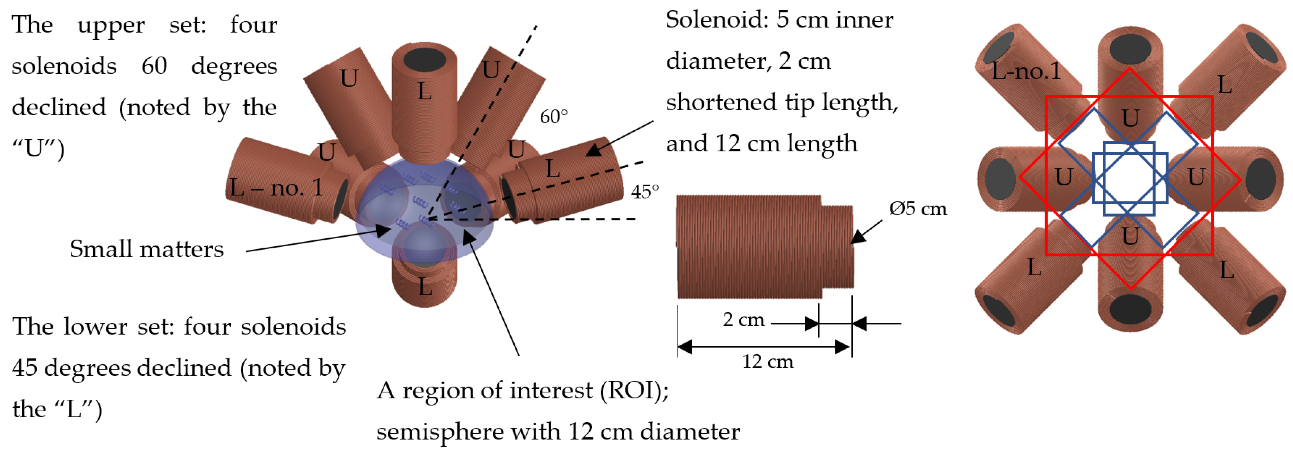
According to the conceptual design, the setup consists of eight solenoids arranged as a nest, and it provides a region of interest or a semispherical space with a dimension of about 12 cm in diameter at the center. Each solenoid has a 5 cm inner diameter and 12 cm length, 320 winding turns of the 1 mm diameter enamel-insulated copper wire, inserted with a permalloy core (1J85 grade: annealed, high saturation (1.5 T), high permeability (1600 H/m), low coercive (1.6 A/m)), as depicted in Figure 4. A core with high permeability can concentrate and empower the magnetic field generated by solenoids. This advantage can reduce the input electrical current supplied to solenoids, leading to a reduction in heat losses (I2R). However, when a highly permeable core-inserted solenoid generates a magnetic field, another nearby solenoid will be affected by mutual inductance, resulting in magnetic noise that can disturb the desired magnetic field. The structure of solenoids is consequently shortened at one end tip in order to eliminate noise.

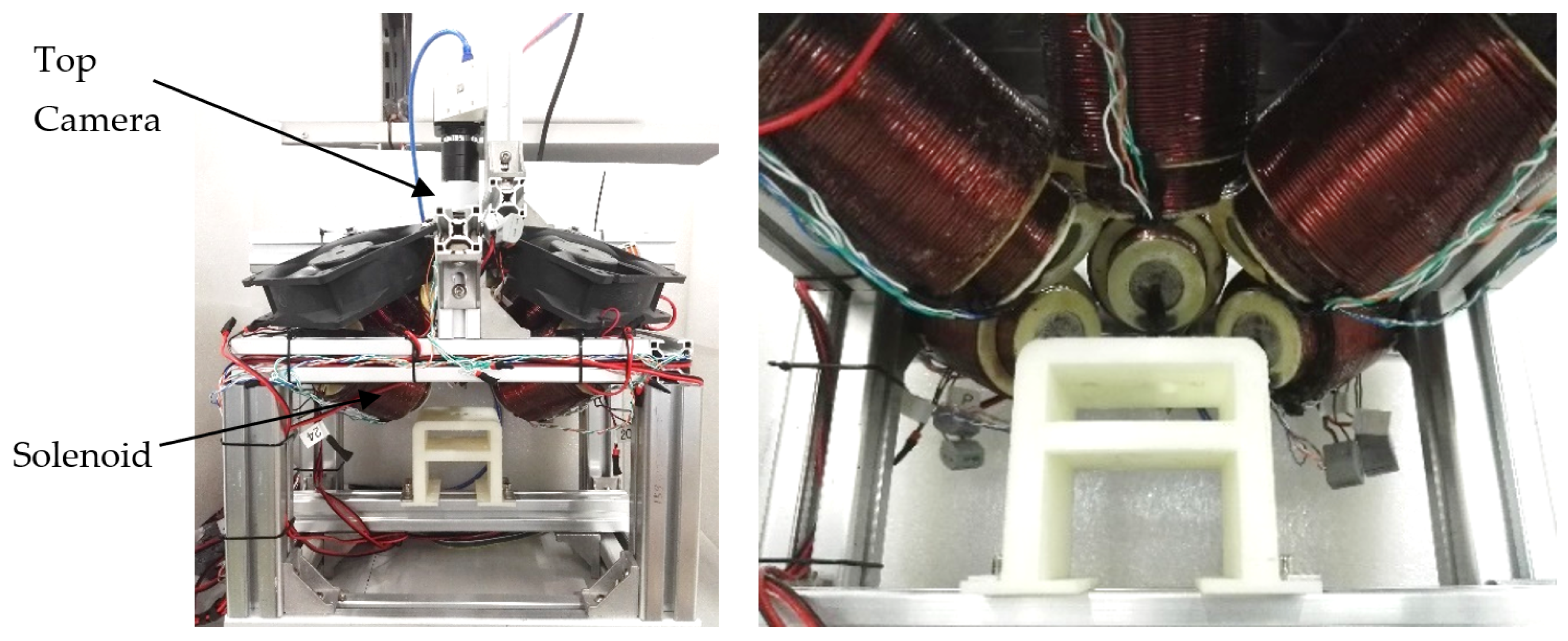
The input electric current supplied into each solenoid is individually operated by four current drivers (Syren 10 by Dimension Engineering, Hudson, OH, USA; 2 channels per each, 25 kHz, 30 V/10 A), and the drivers are all connected with a power supply (SIEMENS GR60 with 40 A/48 V, Siemens, Leipzig, Germany). An amount of input electrical current, including the flowing direction, is commanded via a custom microcontroller with 8-bit-packeted-serial communication controlled by a GUI running on a computer. A Hall effect sensor (Honeywell SS495, range: −67 mT–+67 mT) is attached at each tip of the core to measure the magnetic field during operation. One of the CMOS cameras with a zoom lens (working distance of 6–120 mm and 1.6 mm depth-of-field) is mounted at the top of the setup in order to observe the position and action of a small piece of matter within the region of interest. Another camera is set up at the back of the setup for a back view, perpendicular to the top camera.

The use of eight permalloy core-inserted solenoids results in a linear behavior of the magnetic field generated by the system with respect to the input currents as long as the cores are operated within its linear saturation region. An empirical study is used to verify the linearity of the magnetic field along the x-, y-, and z-directions: $B_x$, $B_y$, and $B_z$, at the center of the ROI as a function of the input electric current supplied into one single solenoid. Since the configuration has geometrical symmetry, it is possible to calculate a map of the magnetic field precisely for all solenoids. Consequently, the magnetic field of all solenoids is measured at other positions of the ROI for mapping the change in magnitude in order to facilitate real-time generated multiplier during control, which is described next. In Figure 5, the hysteresis curve of one single solenoid (no. 1 in Figure 2) in the configuration is plotted as the magnetic field against the input electric current from −10 to 10 A. The magnetic field is measured by using a gaussmeter GM-08 Hirst for three axes. The plot clearly shows no perceivable hysteresis below 8 A and behaves in quasi-linearity. Above 8 A, the magnetic field slightly changes in magnitude. For values above 10 A, the magnetic field is not reported here due to non-linear behavior and high heat loss generation. The result confirms the validity of the linear behavior of the setup, and it facilitates the use of the multiplier for input electric current to generate a constant magnetic field at arbitrary positions over the entire ROI. Especially for 3D-motion control, the constant magnitude of the magnetic field can stabilize the locomotion of the powered matter and lower error in slip, including drift.

According to Figure 5, the magnetic field that exerts a magnetic force on a cylindrical piece of matter (300 µm diameter, 1 mm length) can be simply calculated by following Equations (4) and (6). The magnetic moment of the cylindrical matter is about 4200 ± 500 A·m², as measured by VSM (Vibrating Sample Magnetometer). The magnetic field gradient is estimated by means of the magnetic field at two different points over the distance. Thus, for cases where the cylindrical matter is at the common center point of the ROI, the magnetic force is reported in

Table 1. The magnetic force exerted by the magnetic field of one single solenoid on a cylindrical piece of matter * at the common center point of the ROI under 1 A input electric current.

Force (×10 µN)	Coil 01	Coil 02	Coil 03	Coil 04	Coil 05	Coil 06	Coil 07	Coil 08	Maximum Force of 15 mT (×10 µN)
Fx	−1.385	+1.385	+1.385	−1.385	~0	+1.299	~0	−1.299	7.202
Fy	+1.385	+1.385	−1.385	−1.385	+1.299	~0	−1.299	~0	7.202
Fz	+1.959	+1.959	+1.959	+1.959	+2.401	+2.401	+2.401	+2.401	12.485

* A cylindrical matter is fabricated with NdFeB microparticles (average size: 50 μm) and 40 A shore hardness rubber under the ratio 1:1, and the mixture is processed to have a dimension of about 300 µm diameter and 1 mm length. The magnetic moment is about 4200 ± 500 A·m², and a 15 mT magnetic field is generated by a 5 A input electric current.

. The maximum (15 mT at 5 A input electrical current) is about 72.02 µN for the x-direction, 72.02 µN for the y-direction, and 124.85 µN for the z-direction.

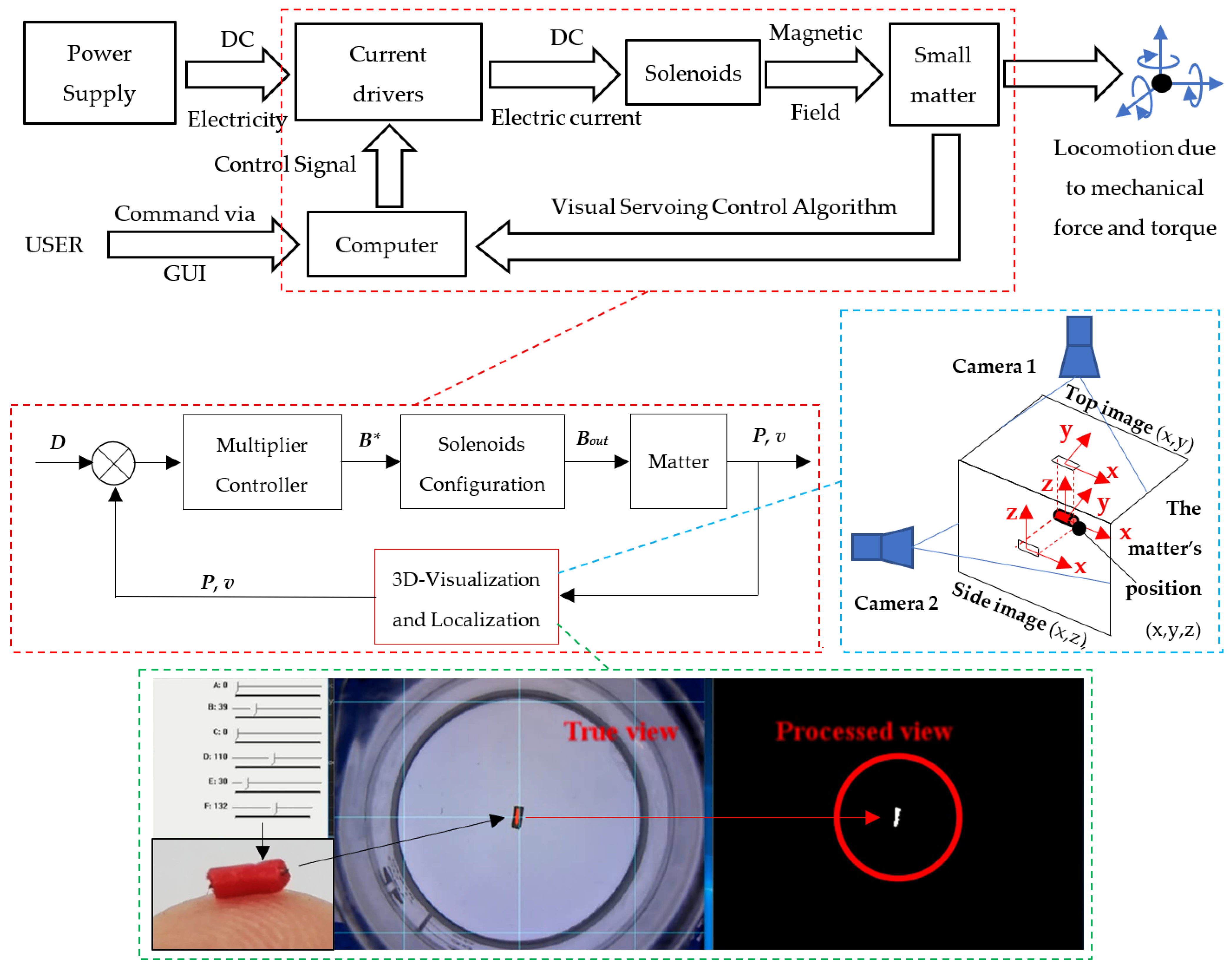
To control magnetic field generation, trilinear interpolation was applied to calculate the magnetic field over the entire ROI in order to define a multiplier of the input electric current matrix supplied into eight solenoids, according to Equation (7). It is straightforward to use the interpolation approach during real-time control. It works because the pose of the piece of matter in the boundary is known. The control algorithm based on visual servoing is applied to track the matter, localize a present coordinate of the matter, and then compute a proper magnetic field to power the matter for precision and to stabilize the motion of the matter. Under the facilitation of quasi-linearity, the precision of motion can be achieved significantly. The working process of the system is presented in the chart in Figure 6. For the 3D-motion control of the matter to arbitrary positions within the workspace, direction, frequency, and speed are commanded via the GUI developed using Python Version 3.9. Firstly, the control GUI allows users to adjust RGB (red, green, blue) or HSB (hue, saturation, brightness) values to match the true color of the matter for accurate detection. Since the matter moves, two cameras capture an image of the matter on different planes: a 2D position (x, z) for the top camera and a 2D position (x, y) for the side camera, and merge them into a 3D position (x, y, z). Finally, when realizing the position of the matter in the x-, y-, and z-coordinates, a multiplier according to that position is activated to gain up or down input electric current for a proper magnetic field to maintain the constant direction and velocity of the matter. Straightforwardly, in the actual control, the bridge that correlates the theoretical concept to the real world is the use of Equations (7) and (8). The matrix 𝒜, which contains the matrix G and K, functions as a real-time generated multiplier for the matrix I to generate force and torque. The matrix I acts as a valve that increases or decreases the magnetic field of each solenoid, resulting in a controllable magnetic field by means of the superposition technique. This concept is very useful in stabilizing the matter’s motion. For example, a piece of matter will move faster when it is close to a magnetic source. The control algorithm can reduce the supplied input electric current to prevent such an issue. For general use, the magnetic field defaults to 15 mT under 5 A input electric current, but it is adjustable when there are gains up or down in the input electrical current. Additionally, one might ask how much force and torque is required to control the matter at that moment. It is possible that not every single piece of matter has the same property. In cases where there is no knowledge of the matter’s magnetic moment, it is recommended to apply a force magnitude strong enough to levitate the matter and adjust the input electric current until the matter is stably located at the center of the ROI. Such a magnitude of force is appropriate for motion control because it can overcome all unwanted factors (e.g., gravity, viscous drag).

Finally, in short, from the design step to implementation, all the above specifications are deliberated based on energy losses as a critical problem in decreasing the performance of electromechanical devices. Those losses are then fixed, which are ohmic losses (I²R), losses in the magnetic core (e.g., hysteresis loss, eddy current loss), and losses in the mechanical system due to movement (e.g., friction, windage, fluidic loss). For ohmic losses, the solenoid is carefully designed to handle both I (input electric current) and R (resistance) components, which majorly lead to heat generation. The I component can generate heat with power two, so the permalloy core with high permeability is used to empower the magnetic field with the lower input electric current if compared with the solenoid with no core. The R component directly relates to the diameter of the copper wire used to wind a solenoid. A smaller diameter will result in a higher resistance. Another concern is about the operating temperature of solenoids. Since the temperature is high, above 90 degrees Celsius, the magnetic field decreases and fluctuates. The fan cooling system is set up to relieve heat. Consequently, the 10 A input electric current generates 90 degrees Celsius within 20 min, but the input electric current at 5 A generates 90 degrees Celsius within one hour. Thus, 5 A is set as the default value of the input electric current. A single solenoid with 5 A input electric current generates a magnetic field of about 15 mT, which is enough to power the piece of matter. The next is the losses in the magnetic core during it is magnetized. The core material is permalloy with high permeability, high saturation, and low coercive, so this type of loss is the least effective. The last are losses due to the movement of the matter. This type of loss mostly appears in terms of friction on the surface and medium where the matter interacts. It can be handled with the control algorithm. For example, visual servoing can track or indicate the present coordinate of the matter in the ROI in order to calculate a proper magnetic field. In the case of friction in a medium, the viscosity will affect how difficult it is for the matter to move. However, strengthening the magnetic field can overcome this problem significantly.

4. System Demonstration Using 3D-Controllable Motion

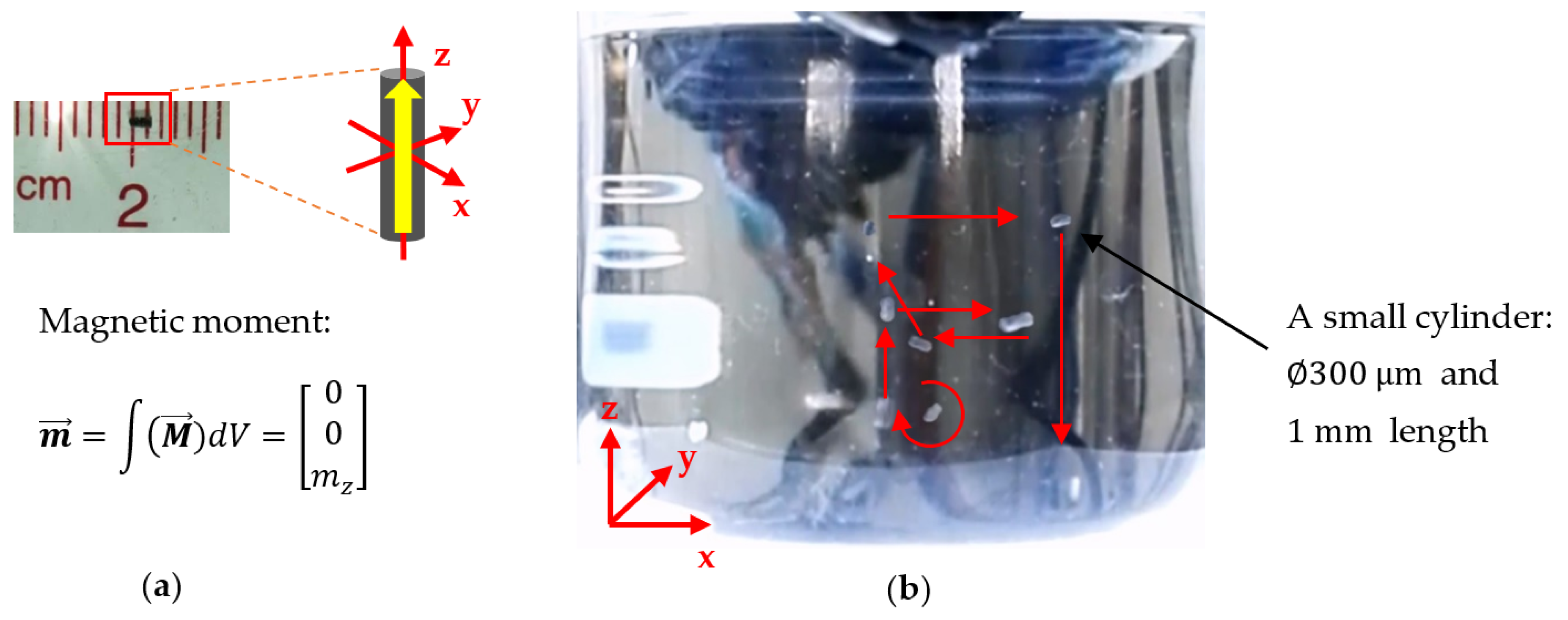
Based on the theoretical concept of electromechanical energy conversion, there are two mechanical variable outputs, which are force and torque, through the medium of the electromagnetic field. Two types of matter that need different control aspects are chosen to validate the feasibility of the system. As depicted in Figure 7, a small piece of matter, made of NdFeb-elastomer with a cylindrical shape and a 300 µm diameter and 1 mm length, magnetized along the axial axis, is subjected to test the conversion of electric energy into mechanical energy through its 3D motion. The cylindrical matter is placed in a 10 cst. silicone oil bath set up in the ROI among the solenoids. Since the input electric current is supplied to each solenoid, the configuration is able to generate the resultant magnetic field, which is controllable in both direction and magnitude by means of the superposition technique. With this aspect, the matter is magnetically navigated to perform 6-DOF motion (translation by force, rotation by torque) within the ROI effectively. When the matter experiences the upward magnetic field, it immediately moves upward. Under the leftward magnetic field, it moves leftward. That is, as long as the generated magnetic field converted from electrical energy is strong enough, we can manipulate and direct the matter to arbitrary positions within the 3D space upon demand. Faster and slower movement is adjustable with an increase or decrease in input electric current, including the flowing direction. In addition, for torque control, when the resultant magnetic field dynamically rotates clockwise or counter-clockwise, the matter responds to the actuation with self-rotation (Supplementary Video S1).

The configuration shown in Figure 8 demonstrates the generation of the continuously dynamic magnetic field to manipulate another small piece of matter to perform a different movement. Since input electric current is supplied to each solenoid under the function of sine and cosine over time, the direction of the resultant magnetic field starts rotating, resulting in a rotating magnetic field or continuous torque. With this aspect, a small piece of matter can rotate according to the rotational direction of the resultant magnetic field. As shown in Figure 8b, a helical-shaped body with a 1 mm diameter and 6 mm length, made of Fe-Ni material, can spin about its axial axis under the rotating magnetic field that exerts a continuous magnetic torque to drive the helix. When the rotational frequency of the resultant magnetic field is faster, it accelerates the spin and simultaneously propels upward along the vertical axis. In addition, when the resultant magnetic field rotates about another axis, the helix is synchronized to rotate and propel about the horizontal axis, as depicted in Figure 8c. Its motion behaves as the rotation for forward propulsion (Supplementary Video S2).

5. Discussion

The result of applying electromagnetic energy to power a small piece of matter is feasible and effective for further applications. The configuration of solenoids is able to generate the magnetic field upon demand in all directions and magnitudes. Several findings of this study can improve the performance of the configuration. First, because the magnetic field is a product of running electric current in copper wire, heat due to electric resistance in the wire is proportional to the magnitude of the input current and the amount of time operating the setup. The higher the input electric current, the hotter the solenoid. Since the solenoid is hotter, the magnitude of the magnetic field is inconstant dramatically. In the experiment, without a cooling unit, the working temperature is measured at a maximum of 92 °C after 15 min of operating time and a 5 A input current supplied to a solenoid. In addition, increasing the copper wire diameter is another solution to decrease electric resistance, but it comes with a much larger gap between winding wires. Second, an iron core or soft magnetic core is another solution to treat heat loss as well as empower the magnetic field. A solenoid with a soft iron core can generate a magnetic field stronger than a solenoid with an air core by about 1.5–3 times depending on the core material. All the above issues are already fixed, and the performance is much better. For example, after setting up a fan-cooling unit to the configuration, the operating temperature and heat loss in the solenoids are much reduced. As observed, the input electric current of about 10 A generates 90 degrees Celsius within 20 min, and the input electric current of 5 A generates 90 degrees Celsius within 1 h. Third, in fact, there are several options to control an accurate magnetic field and its distribution by strategies such as a fitted dipole model of the ROI [21], Finite Element Analysis (FEA) [22], and a real-time computational model based on the Biot–Savart law [23]. These protocols can be applied for the precise motion of the matter. Because the control algorithm is used to generate a proper magnetic field, path following, path planning, and machine learning can be used to enhance the precise motion of the powered small matter. These additional functions have promise for use in the case of medical applications, especially in cases where the clinician accurately navigates the matter as a small machine for therapy at a target. For example, in an endoscopy system, the controllable capsule can vibrationally move along a desired path to a targeted position under the response of an internal magnetic mechanism embedded inside the body to the external magnetic field. This is a potential method for biomedical intervention [24,25,26].

This work was conceptualized with the idea that it would be better to start working from the basic concept in order to cover all the demands of magnetic power. It was then deliberately designed corresponding to the concept of electromechanical energy conversion. Losses were considered, eliminated, and compromised step-by-step with the purpose of obtaining rule-obeyed hardware, and even the simple control technique can deliver a great outcome. For example, under the same input electric current, this work can generate a higher magnitude of the magnetic field, whereas the size is much smaller, including fewer specifications. The solenoid used in this work is just 12 cm long, but the solenoid used in another other work [27] was 21 cm long. This would indicate that energy loss management can improve performance significantly. Moreover, in the motion of a helical piece of matter, due to a quasi-linear magnetic field, magnetic torque is nearly pure to stably drive the helix in all possible directions without nutation and precession due to no interfering force. In addition, an open-loop controller can be applied to control the matter’s motion, but errors will be noticed from motion close to the wall and magnetic sources, lacking uncontrollable velocity, and drifting.

The evaluation of system performance in terms of precision control is not straightforwardly presented in a quantitative context with practical results, but instead, the 3D motion of the matter reported in Section 4 (system demonstration) can be considered to assess the performance. Typically, a magnetic source such as a bar magnet, a solenoid, etc., generates a magnetic field in all directions, which pulls a magnetic-responsive object toward the self-dipole axis. Since the proposed system consists of eight solenoids arranged as a nest, the difficulty in control is related to commanding each solenoid to generate an unequal magnetic field in order to eliminate errors in the movement of the controlled matter. For example, to magnetically levitate a piece of matter, four solenoids of the upper set are operated. That is, four magnetic sources are operated that behave as four vector fields of magnetic dipoles. We can consider that if the controlled matter is not located at the center point of the ROI, it will move upward because the resultant magnetic field of four sources pulls it upward, but slowly, and it acceleratedly bends toward the nearest solenoid because the stronger gradient of the nearest solenoid forces the matter. On the other hand, the control algorithm facilitated by the visual servoing technique will slowly decrease the magnetic field of the nearest solenoid to a value lower than others in order to prevent that effect according to the matter’s position. As shown in Supplementary Video S1, in all directions, the cylindrical piece of matter straightly and constantly moves without drifting, and no swaying is noticed during the rapid change in movement. Also, in Supplementary Video S2, neither precession nor nutation exists during the change in the rotation axis of the helix from the vertical axis to the horizontal axis due to changes in torque. These results can represent and clarify the control performance for precision of motion significantly.

6. Conclusions

The energy conversion principle is widely used in different applications such as generators, wind turbines, motors, etc. Apart from the common use, this work proposes an advanced application based on the conversion from electrical energy to mechanical energy through the controllable magnetic field to remotely and wirelessly manipulate the locomotion of a small piece of matter in three-dimensional space. The configuration of eight solenoids as an electromechanical energy conversion device is invented to prove the feasibility of such an aspect for remote wireless powering. It is capable of generating a magnetic field in all directions and magnitudes by means of the superposition technique. The visual servoing-based control algorithm is integrated to localize a coordinate of the powered matter in order to produce the magnetic field upon demand properly. The results show that small matter can move across three-dimensional space effectively under magnetic manipulation, which adopts the concept of electromechanical energy conversion. This contribution is widely applicable in medical applications operated by a controllable tiny machine. The concept still allows for the implementation of small actuators and mechanisms set up inside a small engine for further applications such as a micro-propeller in a tiny pump, a micro-turbine in a small submarine, etc.

References

1. Gieras, J.F. Introduction to Electromechanical Energy Conversion, 1st ed.; CRC Press: London, UK, 2016. [Google Scholar]
2. Kumar, P.; Huang, Y.; Toyserkani, E.; Khamesee, M.B. Development of a Magnetic Levitation System for Additive Manufacturing: Simulation Analyses. IEEE Trans. Magn. 2020, 56, 8000407. [Google Scholar] [CrossRef]
3. Batista, D.S.; Granziera, F.; Tosin, M.C.; de Melo, L.F. Three-Axial Helmholtz Coil Design and Validation for Aerospace Applications. IEEE Trans. Aerosp. Electron. Syst. 2018, 54, 392–403. [Google Scholar] [CrossRef]
4. Yang, L.; Wang, Q.; Zhang, L. Model-free trajectory tracking control of two-particle magnetic microrobot. IEEE Trans. Nanotechnol. 2018, 17, 697–700. [Google Scholar] [CrossRef]
5. Denasi, A.; Khan, F.; Boskma, K.J.; Kaya, M.; Hennersperger, C.; Gobl, R.; Tirindelli, M.; Navab, N.; Misra, S. An Observer-Based Fusion Method using Multicore Optical Shape Sensors and Ultrasound Images for Magnetically-Actuated Catheters. In Proceedings of the 2018 IEEE International Conference on Robotics and Automation (ICRA), Brisbane, Australia, 21–25 May 2018; pp. 50–57. [Google Scholar]
6. Yu, J.; Zhang, L. Reversible Pattern Transformation of Paramagnetic Nanoparticle Swarms in Bio-fluids with High Ionic Strength. IEEE/ASME Trans. Mechatron. 2019, 24, 154. [Google Scholar] [CrossRef]
7. Yu, C.; Kim, J.; Choi, H.; Choi, J.; Jeong, S.; Cha, K.; Park, J.-O.; Park, S. Novel electromagnetic actuation system for three-dimensional locomotion and drilling of intravascular microrobot. Sens. Actuators A Phys. 2010, 161, 297–304. [Google Scholar] [CrossRef]
8. Ha, Y.H.; Han, B.H.; Lee, S.Y. Magnetic nanoparticle density mapping from the magnetically induced displacement data: A simulation study. Med. Biol. Eng. Comput. 2010, 48, 139. [Google Scholar]
9. Jeon, S.; Jang, G.; Choi, H.; Park, S. Magnetic navigation system with gradient and uniform saddle coils for the wireless manipulation of micro-robots in human blood vessels. IEEE Trans. Magn. 2010, 46, 1943–1946. [Google Scholar] [CrossRef]
10. Hidalgo-Tobon, S. Theory of gradient coil design methods for magnetic resonance imaging. Concepts Magn. Reson. Part A 2010, 36A, 223–242. [Google Scholar] [CrossRef]
11. Kratochvil, B.E.; Kummer, M.P.; Erni, S.; Borer, R.; Frutiger, D.R.; Schürle, S.; Nelson, B.J. MiniMag: A Hemispherical Electromagnetic System for 5-DOF Wireless Micromanipulation. Exp. Robot. 2014, 79, 317–329. [Google Scholar]
12. Son, D.; Dong, X.; Sitti, M. A Simultaneous Calibration Method for Magnetic Robot Localization and Actuation Systems. IEEE Trans. Robot. 2019, 35, 343–352. [Google Scholar] [CrossRef]
13. Li, J.; Wang, H.; Cui, J.; Shi, Q.; Zheng, Z.; Sun, T.; Huang, Q.; Fukuda, T. Magnetic Micromachine Using Nickel Nanoparticles for Propelling and Releasing in Indirect Assembly of Cell-Laden Micromodules. Micromachines 2019, 10, 370. [Google Scholar] [CrossRef]
14. Petruska, A.J.; Nelson, B.J. Minimum bounds on the number of electromagnets required for remote magnetic manipulation. IEEE Trans. Robot. 2015, 31, 714–722. [Google Scholar] [CrossRef]
15. Go, G.; Choi, H.; Jeong, S.; Lee, C.; Ko, S.Y.; Park, J.-O.; Park, S. Electromagnetic Navigation System using Simple Coil Structure (4 Coils) for 3-D Locomotive Microrobot. IEEE Trans. Magn. 2015, 51, 2067. [Google Scholar] [CrossRef]
16. Carpi, F.; Pappone, C. Stereotaxis Niobe®Magnetic Navigation System For Endocardial Catheter Ablation And Gastrointestinal Capsule Endoscopy. Expert Rev. Med. Devices 2009, 6, 487–498. [Google Scholar] [CrossRef]
17. Bigot, A.; Tremblay, C.; Soulez, G.; Martel, S. Impairment-Based 3-D Robotic Intervention Improves Upper Extremity Work Area in Chronic Stroke: Targeting Abnormal Joint Torque Coupling With Progressive Shoulder Abduction Loading. IEEE Trans. Robot. 2014, 30, 719. [Google Scholar] [CrossRef]
18. Erin, O.; Boyvat, M.; Tiryaki, M.E.; Phelan, M.; Sitti, M. Magnetic Resonance Imaging System–Driven MedicalRobotics. Adv. Intell. Syst. 2020, 2, 1900110. [Google Scholar] [CrossRef]
19. Manamanchaiyaporn, L.; Xu, T.; Wu, X. An Optimal Design of an Electromagnetic Actuation System towards a Large Homogeneous Magnetic Field and Accessible Workspace for Magnetic Manipulation. Energies 2020, 13, 911. [Google Scholar] [CrossRef]
20. Manamanchaiyaporn, L.; Xu, T.; Wu, X. The HyBrid System with a Large Workspace towards Magnetic Micromanipulation within the Human Head. In Proceedings of the 2017 IEEE/RSJ International Conference on Intelligent Robots and Systems (IROS), Vancouver, BC, Canada, 24–28 September 2017; pp. 401–407. [Google Scholar]
21. Spaldin, N.A. Magnetic Materials Fundamentals and Applications, 2nd ed.; Cambridge University Press: New York, NY, USA, 2010. [Google Scholar]
22. Sikorski, J.; Dawson, I.; Denasi, A.; Hekman, E.E.; Misra, S. Introducing Bigmag—A Novel System for 3d Magnetic Actuation of Flexible Surgical Manipulators. In Proceedings of the 2017 IEEE International Conference on Robotics and Automation (ICRA), Singapore, 29 May–3 June 2017; pp. 3594–3599. [Google Scholar]
23. Le, V.N.T.; Nguyen, N.H.; Alameh, K.; Weerasooriya, R.; Pratten, P. Accurate Modeling and Positioning of a Magnetically Controlled Catheter Tip. Med. Phys. 2016, 43, 650–663. [Google Scholar] [CrossRef] [PubMed]
24. Liu, Y.; Islam, S.; Pavlovskaia, E.; Wiercigroch, M. Optimization of the Vibro-Impact Capsule System. J. Mech. Eng. 2016, 62, 430–439. [Google Scholar] [CrossRef]
25. Zhang, J.; Liu, Y.; Zhu, D.; Prasad, S.; Liu, C. Simulation and Experimental Studies of a Vibro-Impact Capsule System Driven by an External Magnetic Field. Nonlinear Dyn. 2022, 109, 1501–1516. [Google Scholar] [CrossRef]
26. Keller, H.; Juloski, A.; Kawano, H.; Bechtold, M.; Kimura, A.; Takizawa, H.; Kuth, R. Method for Navigation and Control of a Magnetically Guided Capsule Endoscope in the Human Stomach. In Proceedings of the 2012 4th IEEE RAS & EMBS International Conference on Biomedical Robotics and Biomechatronics (BioRob 2012), Rome, Italy, 24–27 June 2012; pp. 859–865. [Google Scholar]
27. Kummer, M.P.; Abbott, J.J.; Kratochvil, B.E.; Borer, R.; Sengul, A.; Nelson, B.J. OctoMag: An electromagnetic system for 5-DOF wireless micromanipulation. IEEE Trans. Robot. 2010, 26, 1006–1017. [Google Scholar] [CrossRef]
Figure 1. Scheme of electromechanical energy conversion.
Energies 17 01155 g001
Figure 2. The setup of eight solenoids as an electromechanical energy conversion device. (Left) The 3D view of the setup. (Middle) Coil structure with a 5 cm inner diameter, 2 cm shortened tip length, and 12 cm length. (Right) The top view of the setup. The working distance from the tip of each solenoid to the center of the ROI is equal.
Energies 17 01155 g002
Figure 3. Simulation of magnetic field generation by four solenoids. Green arrows represent the resultant magnetic field due to the superposition technique. (ah) to show the on-demand direction and magnitude of the magnetic field generated by solenoids under the 1 A input electric current. E.g., (b) The 90-degree magnetic field is the product of the magnetic field generated by four solenoids with the direction according to the white arrow. The magnetic field at the center of the ROI (red circle: 12 cm diameter) is reported to be maximum at 3.31 mT.
Energies 17 01155 g003
Figure 4. The setup of eight solenoids arranged as a nest. At the top, a camera is mounted to capture a small piece of matter as well as obtain the location used to feedback to the control algorithm based on the visual servoing technique.
Energies 17 01155 g004
Figure 5. Hysteresis curve of the magnetic field at the center of the workspace plotted against the input electric current supplied to a single solenoid. Note that the net magnetic field at the center along the axial axis of the solenoid is about 15 mT at 5 A.
Energies 17 01155 g005
Figure 6. (Upper) A process to convert electromechanical energy (from electrical energy to mechanical energy) through the 3D-controllable motion of a small piece of matter. (Middle-left) Close loop control using the visual servoing algorithm to generate a magnetic field for 3D locomotion of the matter. Notations: D is the desired direction vector of the controlled matter for the next position. B* and Bout are the desired driving and the generated magnetic field, respectively. P is the position of the matter, which is obtained by the projection of the geometric center. v is the advance velocity vector of the matter, which is adjustable by gaining strength magnetic field. (Middle-right) How two cameras localize the x-, y-, and z-coordinates fed back to the control algorithm. (Lower) The GUI allows a user to adjust the RGB and HSB of the camera visualization to match the true color of the matter in order to avoid out-of-focus errors during control.
Energies 17 01155 g006
Figure 7. The 3D-controllable motion of a cylindrical piece of matter in 10 cst. oil. (a) A small cylinder with a 300 µm diameter and 1 mm length, where the net magnetic moment points along the axial direction are represented by the yellow arrow. (b) The resultant magnetic field manipulates the cylinder to travel in three-dimensional space under the concept of electromagnetic energy conversion. Red arrows define the motion direction of the cylinder.
Energies 17 01155 g007
Figure 8. Controllable rotational motion of a small helix. (a) A small helix with a 1 mm diameter and 6 mm length, where the net magnetic moment points along the radial direction are represented by the yellow arrow. (b) The rotating magnetic field is generated about the vertical axis to drive the helix to propel upward. (c) The rotating magnetic field is generated about the horizontal axis to drive the helix to roll on the horizontal plane. Red arrows define the motion direction of the helix, which rotates by propelling.
Energies 17 01155 g008