Thermal Testing and System Reliability: Transferring Thermal Interactions by Heat Conduction through a Peltier-Based Thermal Coupling System

Abstract

Testing and reliability assessment are crucial aspects when considering the thermal domain’s influence on the overall system. Thermal interactions occur between all subsystems, and their separation can disrupt internal thermal interactions, altering temperature profiles. Evaluating functional system reliability requires accounting for the thermal domain’s impact on temperature-dependent performance and thermal damage limits. However, testing faces challenges due to the lack of a suitable thermal coupling system capable of transferring thermal interactions by heat conduction between spatially separated subsystems. To address this issue, this paper introduces a thermal coupling system that focuses on the control system and its validation through experimental studies. Two scenarios were investigated: (I) the original assembly situation with direct heat transfer between two subsystems, and (II) a spatially separated scenario utilizing the thermal coupling system to establish heat transfer between the subsystems. The evaluation variables are the temperature curves and the deviations between the two scenarios. Two different tests with a different amount of heat flows are carried out. The thermal coupling system utilizes thermal actuators, specifically Peltier devices, to ensure a zero temperature difference between the original contact points. The control system employs both closed-loop and open-loop control to regulate the heat flow and achieve energy conservation between the spatially separated subsystems. The results demonstrate that the described thermal coupling system yields only slight deviations in temperature curves, indicating its applicability for early evaluation of functional system reliability. This research contributes to a better understanding of thermal interactions in complex systems and provides a valuable tool for enhancing overall system reliability through thermal testing and validation.

1. Introduction

One of the most important key challenges in product engineering is the design of reliable systems [1]. Functional reliability denotes a system’s capacity to meet its intended functionality within specified conditions for a specified period of time [2].

In the context of complex systems, achieving system reliability presents significant challenges owing to the profound interactions between the subsystems comprising a single technical system and its surrounding environment or other systems. Consequently, it is imperative to proactively consider those interactions in future applications during the product development phase to account for their potential impact on its reliability. This can be achieved with validation, verification, and testing (VVT) strategies [3].

The thermal domain is important in this context because the temperature-dependent performance of systems and the thermal damage limit can be considered. For instance, temperature-dependent influences in the electrical domain are well known (electric motor, etc.) [4,5,6,7]. Additionally, the temperature dependence in the hydraulic domain can be shown with many examples. The physical properties of hydraulic oil, such as density, viscosity, and dynamic viscosity, are temperature-dependent [8].

There are a lot of environmental testing standards, which focus on the thermal domain [9,10,11]. The thermal domain must be considered in the overall system because thermal interactions occur between all subsystems. Separating the subsystems interrupts the internal thermal interactions and thus the heat flows between the subsystems. A separation of subsystems occurs when physical subsystems, which are firmly connected to each other in their original installation situation, are spatially separated. Another possibility is when one subsystem is present physically while the other system is simulated in the virtual domain, and thus no direct heat exchange is possible. This can happen in the context of X-in-the-Loop (XiL) test benches.

The overall sum of the heat flows in the individual subsystems is altered compared to the original assembly situation when it comes to a separation of the subsystems. This leads to a change in the temperatures. Figure 1 shows the situation with the simplification of the two subsystems A and B. The heat flows ${\dot{Q}}_1$ and ${\dot{Q}}_3$ are representative of heat flows to the environment by convection and heat radiation. The heat flow ${\dot{Q}}_2$ is representative of a heat flow by conduction between the two subsystems.

Figure 1. (a) Scenario (I): Heat flows in the connected subsystems (original assembly situation), and (b) Scenario (II): Heat flows in the spatially separated subsystems, based on [12].

The idea of a thermal coupling system (TCS) is to transfer the unknown heat flow ${\dot{Q}}_2$ between separated subsystems so that a temperature profile as in the original assembly situation is obtained. The thermal coupling system consists of sensors, actuators, and control systems to transfer the unknown heat flow ${\dot{Q}}_2$.

2. Related Work

The following related work from literature is structured using different categories: type of thermal interactions, testing objective, type of heat transfer, and the integration level.

The first category is the thermal interactions that can be transferred via physical separated subsystems, meaning physical–physical interactions. In the context of XiL test benches, physical and virtual subsystems must be connected as well. Therefore, it should not only transfer physical–physical thermal interactions, but also physical–virtual ones. Physical–virtual interactions require the integration of a validated simulation model representing the virtual subsystem. To reduce this complexity and influence, physical–physical interactions are focused as a foundational step to validate the principles and efficacy of a TCS.

The second category is the testing objective. The testing objectives of these investigations can be properties or functions in the context of reliability testing. The tests, which are carried out with a thermal coupling system, are aimed at checking that the function is fulfilled. The determination of thermal properties does not have any role to play here.

The third category is the type of heat transfer. The heat transfer forms that can be considered are thermal conduction, forced convection, natural convection, and thermal radiation. Since a separation of subsystems interrupts the internal interactions, heat conduction must be considered.

The fourth category is the integration level. When the test object is integrated in the overall system, the interactions between all the subsystems must be transferred. This is common in the context of XiL test benches. The coupling system should therefore influence both subsystems which are connected by it. Component tests focus solely on the effects on the individual component, but not on the interactions due to the integration into the overall system.

Gross-Weege et al. [13] describe a control design for a thermal hardware-in-the-loop test bench. It is possible to transfer thermal interactions between physical and virtual subsystems, although the virtual system is restricted here as an environmental boundary condition. The testing objective is to evaluate the functional fulfillment in the overall system. The transferred heat transfer form is forced convection. This is suitable for thermal managements systems in automotive.

Eisele [14] describes a slightly different approach. The focus is on the validation environment for the design of cooling concepts in battery module development. The heat transfer form is forced convection as well. Single physical battery cells can be thermally and electrically coupled to a real-time simulation of the battery module with the described coupling system. The XiL approach is used to test the functional performance of individual subsystems such as the battery cells that are integrated into the overall system.

Christen et al. [15] describe a test method for the thermal characterization of Li-ion cells and the verification of cooling concepts. The system is investigated in the overall system. The heat transfer form is conduction. They describe a method to determine the entropic heat coefficient of battery cells through heat flow measurements. Their testing objective is therefore to determine thermal properties. Their test bench consists of temperature and heat flow sensor. However, the physical–virtual interactions are not transferred.

Bui et al. [16] describe an advanced Hardware-in-the-Loop battery simulation platform for the experimental testing of battery management system. A physical battery cell is electrically connected to virtual battery cells. Thermal interactions between the physical and virtual battery cells cannot be transferred. However, a controllable climate chamber simulates the environmental temperature and is kept constant for the described study.

There are several descriptions of standardized tests that analyze the thermal properties of single components: DIN EN 12667 [17], DIN EN 821 [18], and ASTM C518 [19]. All of them focus on the properties in the context of heat conduction. All of them describe methods to keep the test environment at a specific temperature or temperature gradient.

Lucas et al. have contributed to the field of thermal management systems through their work detailed in three separate papers [20,21,22], focusing on the use of Peltier devices. While these studies offer valuable insights, it is noted that the thermal interactions facilitated by these systems are not entirely transferred. The primary objective outlined by Stephen et al. is the development of a thermal management system designed to prevent failure in electrical insulation. They identify that high temperatures can lead to condensation, which pose a significant risk of failure. The example given is an electric engine. The implemented thermal management system should avoid such failure by cooling down the electric engine. There is no equipment to transfer thermal interactions in the context of spatially separated subsystems.

Sun et al. [23] describe a testing framework for virtual battery pack-based battery management systems. It is based on a hardware-in-the-loop testing concept. The integration level is therefore the overall system. The testing objective is to investigate the battery management system function. It includes a thermal model. However, this lacks integration into the overall system. Thermal interactions are not transferred between the virtual battery and the surrounding subsystems.

Troxler et al. [24] describe a test bench that can control the thermal boundary conditions of Li-ion cells using Peltier devices during electrical testing. It is possible to induce thermal gradients from outside to the Li-ion cells. It is therefore integrated into the overall system. Nevertheless, only the effect on the Li-ion cell can be achieved. There is no action back to the surrounding system; therefore, it only partially transfers the thermal interactions.

Kulikov et al. [25] describe an X-in-the-Loop test bench to test a thermal management system for electric cars. A physical thermal management system is connected to a virtual model of the electric drive components. Therefore, interactions between physical and virtual subsystems are transferred. The thermal and hydraulic behavior is tested in the overall system. The heat transfer form is forced and natural convection.

Leitenberger et al. [8] describe a concept of a TCS to consider thermal interactions between spatially separated subsystems. The testing objective is to evaluate the functional fulfillment in the overall system. The concept is shown with a simulation. They showed the feasibility of the concept but were not able to validate it yet.

In Table 1, it can be seen that none of the related work meets all the required categories, but only part of them. While the state of research shows a variety of approaches which come with their individual strengths, none of the previously described works are fulfilling all the categories that are needed for the TCS, nor are they physically validated.

Table 1. Related work which implements the key categories for a thermal coupling system for the transfer of thermal interactions by heat conduction between physical subsystems (empty circle = not applicable; half-filled circle = partially applicable; fully filled circle = completely applicable).

Publications	Thermal Interactions		Research Objective		Heat Transfer Forms				Integration Level
	Physical–Physical	Physical–Virtual	Properties	Functions	Thermal Conduction	Forced Convection	Natural Convection	Thermal Radiation	Component	Overall System
Gross-Weege et al. [13]
Eisele [14]
Christen et al. [15]
Bui et al. [16]
DIN EN 12667 [17], DIN EN 821 [18], ASTM C518 [19]
Lucas et al. [20,21,22]
Sun et al. [23]
Troxler et al. [24]
Kulikov et al. [25]
Leitenberger et al. [12]

The research problem is that there is no validated TCS to transfer thermal interactions by heat conduction for thermal testing to investigate system reliability. Regarding physical–virtual interactions, these require the integration of a validated simulation model representing the virtual subsystem. However, we have not included physical–virtual interactions in this manuscript in order to avoid complexity and to ensure clarity. Our aim was to first validate the principles and efficacy of the TCS in a physical–physical context.

This leads to the following research question: How can thermal interactions by heat conduction be transferred between spatially separated physical subsystems in order to perform an early assessment of functional system reliability?

Building upon the previous works, this paper describes a thermal coupling system (TCS) for the transfer of thermal interactions by heat conduction between physical subsystems.

3. Materials and Methods

This chapter explains the details of the experimental setup. It includes a description of the experimental design, which covers the scenarios and test cases used. TCS is explained, which transfers thermal interactions through heat conduction. The materials and components used in the tests are also described.

3.1. Experimental Design

Two different scenarios are compared to each other. Scenario (I) represents the original assembly situation and therefore serves as a reference to validate the thermal coupling system. Scenario (II) is the use-case when two subsystems are spatially separated and connected via a TCS. Figure 2 represents the two scenarios.

Figure 2. (a) Test setup of scenario (I) as reference, and (b) test setup of scenario (II) as thermally coupled subsystems.

For simplification, the subsystems will be considered only in the thermal domain. Power losses in the individual subsystems are described as heat sources in the modelling context. Those are described as ${\dot{Q}}_A$ for subsystem A with the power losses occurred through the resistance R. Thermal radiation and free convection are considered. These are represented as an external resulting heat flow ${\dot{Q}}_{amb,A}$ and ${\dot{Q}}_{amb,B}$. The heat flow ${\dot{Q}}_{cond}$ through conduction between the subsystems A and B is considered separately to be investigated in the thermal coupling systems. The contact resistance between subsystems A and B is to be neglected. The numbers in the black boxes are temperature sensors.

The equations describing the energy balance for subsystems A and B are represented by (1) and (2). The thermal energy U that is stored within the subsystem leads to the temperature increase.

$$\frac{d{U}_A}{dt}={\dot{Q}}_A-{\dot{Q}}_{amb,A}-{\dot{Q}}_{cond}$$

(1)

$$\frac{d{U}_B}{dt}={\dot{Q}}_{cond}-{\dot{Q}}_{amb,B}$$

(2)

Two test cases were carried out, which differ in the applied heat transfer ${\dot{Q}}_A$. The first test case transfers 100 W to investigate the behavior for high heat transfers and therefore for high temperature changes. The second test case transfers 50 W to investigate if there is any influence on the amount of heat is transferred.

3.2. Thermal Coupling System (TCS) for Heat Conduction

The description of the thermal coupling system in this chapter is based on the publication of Leitenberger et al. [12].

Due to boundary conditions, original contact points 2 and 3 (see Figure 2) must have identical temperatures. To ensure the thermal coupling condition, it is imperative that the temperature difference between the two initial contact points is zero.

$$\Delta T_{2,3}=0,$$

(3)

To couple temperature sensors 2 and 3 thermally, two thermal actuators need to be placed on either side of the original contact surface to transfer the heat flow ${\dot{Q}}_{cond}$. Peltier devices can be used as thermal actuators due to their ability to rapidly heat or cool a surface by simply reversing the direction of the electric current. They are also known as Peltier coolers or thermoelectric coolers (TECs) and utilize the Peltier effect to transfer heat between two different surfaces.

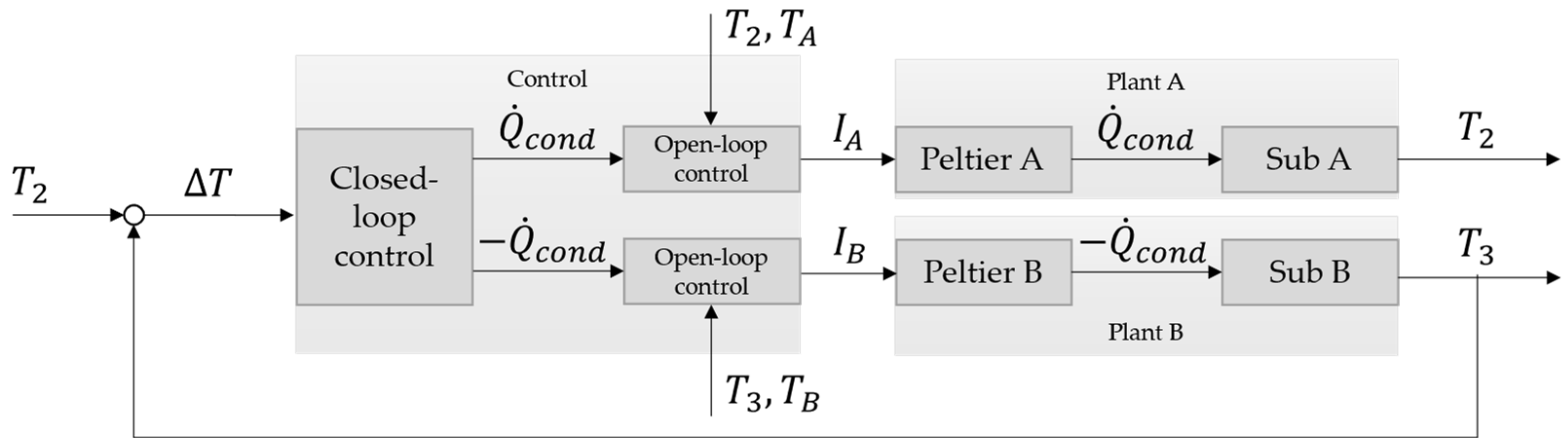
The control system is based on two parts. One closed-loop control controls the two parts of the thermal coupling systems. Due to the physical effects of the Peltier devices, there is an open-loop control for each single Peltier device.

The closed-loop control is implemented as a PI control. The control difference corresponds to the thermal coupling condition. The heat flow ${\dot{Q}}_A$ serves as the independent variable. In accordance with energy conservation, the heat flow that is removed from one subsystem must be supplied to the other subsystem in the same amount. The Peltier devices are capable of supplying and removing heat flows. The control variable for this control system is the electric current I of the Peltier devices. However, the behavior is dependent on the direction of the heat flow. This is the reason for the open-loop control to fulfill the energy conservation.

The open-loop control follows a model-based approach and can be seen as feedforward control. For this purpose, the Peltier devices are modelled. Depending on the amount of heat flow ${\dot{Q}}_x$ is extracted from the applied subsystem and which heat flow ${\dot{Q}}_Y$ is dissipated, different temperatures, $T_X$ and $T_Y,$ occur on the two sides of the Peltier device. To carry this out, an electrical power P must be supplied to the Peltier device. Figure 3 shows the schematic structure of the Peltier device.

Figure 3. Schematic structure of a Peltier device based on [12].

Neglecting the thermal mass of the Peltier device results in an energy balance according to Equation (4):

$${\dot{Q}}_Y={\dot{Q}}_X+P,$$

(4)

The heat flow $\dot{Q}$ generated by the thermoelectric effect can be described by the following:

$$\dot{Q}=S\ast T\ast I,$$

(5)

The Seebeck coefficient S is mainly determined by the choice of semiconductor pairs used. The Peltier device’s mass is negligible, but heat conduction is crucial. When a Peltier device experiences a temperature difference between its two sides, heat conduction generates an opposing heat flow. This opposing flow can become significant, to the point where the net heat flow can become zero or even reverse, despite a higher current I. Equations (6) and (7) describe the net heat flow of sides $X$ and $Y$ in the Peltier device [26]:

$${\dot{Q}}_X=S{T}_{X}I-\frac{1}{2}{I}^{2}R+\frac{\left(T_X-T_Y\right)}{R_{\theta }},$$

(6)

$${\dot{Q}}_Y=S{T}_{Y}I+\frac{1}{2}{I}^{2}R+\frac{\left(T_X-T_Y\right)}{R_{\theta }}$$

(7)

The parameter R represents the electrical resistance and $R_{\theta }$ the absolute thermal resistance due to conductivity. Based on these equations, the open-loop control determines the current I that has to be applied to set the heat flow ${\dot{Q}}_{cond}$. Depending on the application, the heat flow ${\dot{Q}}_{cond}$ can be ${\dot{Q}}_X$ or ${\dot{Q}}_Y$.

In order to achieve the required performance of the Peltier device, a cooler or heater can be added to reduce the temperature difference between the two sides, X and Y. These devices have a two-point control and become active when the temperature difference is bigger than 0.5 K. Due to this experimental design, a cooler is attached on the Peltier device of side A and a heater on the Peltier device of side B.

The control system of the thermal coupling system is shown in Figure 4. For the sake of clarity, the two-point control to acclimatize the Peltier devices have been left out. The subsystem and the Peltier device form the plant of this system.

Figure 4. Control system of the thermal coupling system to consider thermal interactions between physical subsystems.

The P and I values of the closed-loop control were determined with the help of the simulation of Leitenberger et al. [12]. Through simulative testing, the parameters were manually optimized according to the criteria of stability and speed. This resulted in a value of P = 5 and I = 10 for this system.

3.3. Material

Peltier devices QuickCool QC-161-1.6-15.0M (Quick-Ohm Küpper und Co. GmbH, Wuppertal, Germany, [27]) are used as thermal actuators. The Seebeck coefficient S has a value of $0.05 \mathrm{V}/\mathrm{K}$, the electrical resistance R of 1.14 Ω, and the absolute thermal resistance $R_{\theta }$ of $0.625 \mathrm{K}/\mathrm{W}$. Depending on how they are connected, heat flows can be removed or added. The programmable DC power supplies (EA-PS 9040-20T, EA Elektro-Automatik GmbH & Co. KG, Viersen, Germany, [28]) are used to control the electrical currents $I_A$ and $I_B$ for the Peltier devices.

The heater consists of eight TO126 high power resistors (TCP10S-C10R0FTB, TRU COMPONENTS, Hirschau, Germany, [29]) with an electrical resistance R of 10 Ω. The rating power is 20 W for a single resistor. The resistors are connected so that a thermal power of more than 100 W can be achieved.

Six temperature sensors (Thermocouple type J, class 1, IEC 60584-1, [30]) are used to acquire the temperature profile across the subsystems. The tolerance in the used temperature range is ±1.5 °C. One sensor is attached to each end face. The temperature sensors are sunk about 10 mm deep into the material through small holes. In addition, a temperature sensor is attached to the Peltier device on the side facing away from the subsystem in order to detect the temperature difference between the two sides of the Peltier device. This refers to sides X and Y in Figure 3.

Heat transfer compound (KP 96 Keratherm, KERAFOL Keramische Folien GmbH, Eschenbach, Germany, [31]) is used between the different parts to reduce the contact resistance.

Subsystem A and B have the geometric dimensions of 150 mm × 70 mm × 50 mm. The subsystems A and B are each made of aluminium alloy EN AW-6061. This aluminium alloy has a density ρ of $2.7 \mathrm{g}/\mathrm{cm}3$, a specific heat capacity $c_p$ of $1106 \mathrm{J}/\left(\mathrm{kg}\ast \mathrm{K}\right)$, and a thermal conductivity λ of $172 \mathrm{W}/\left(\mathrm{m}\ast \mathrm{K}\right)$ [32].

The test bench is controlled by the measurement and control system ADwin-Pro2 (Jäger Computergesteuerte Meßtechnik GmbH, Lorsch, Germany, [33]). The sample and record frequency of the system is 1 kHz. The temperature sensors are connected via the measuring amplifier Pro II-TC-8-ISO [34]. This has a measuring resolution of 0.1 °C. Each temperature sensor is individually calibrated. Compensation cables have not been used. The temperature values are used with a 4th order zero-phase Butterworth filter with a cut-off frequency of 5 Hz.

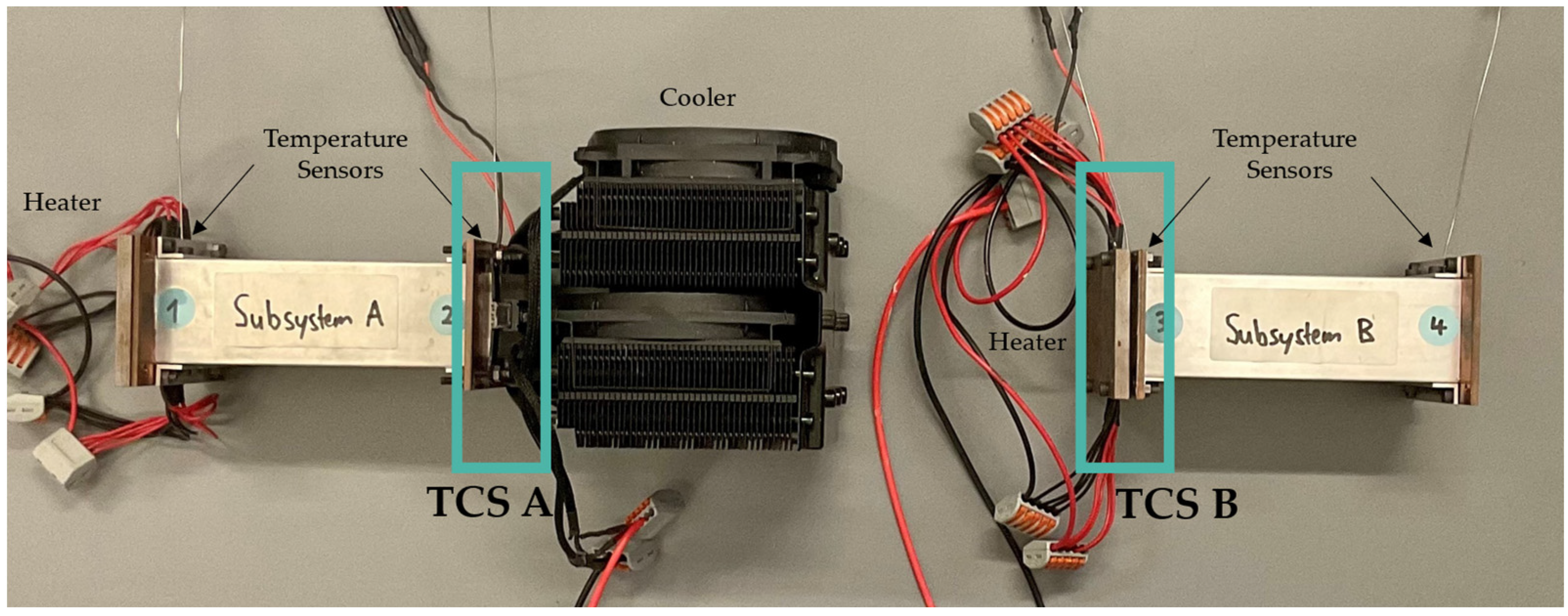
The ambient environment is kept constant by a climate chamber (Unistat 425, Peter Huber Kältemaschinenbau SE, Offenburg, Germany, [35]). Figure 5 shows the setup of scenario II.

Figure 5. Test bench setup of scenario II inside the climate chamber.

4. Results of the Experimental Study

In this chapter, the results of the validation of the thermal coupling system are presented. The thermal coupling system is validated by comparing the deviations between the temperatures.

4.1. Test Case 1: 100 W

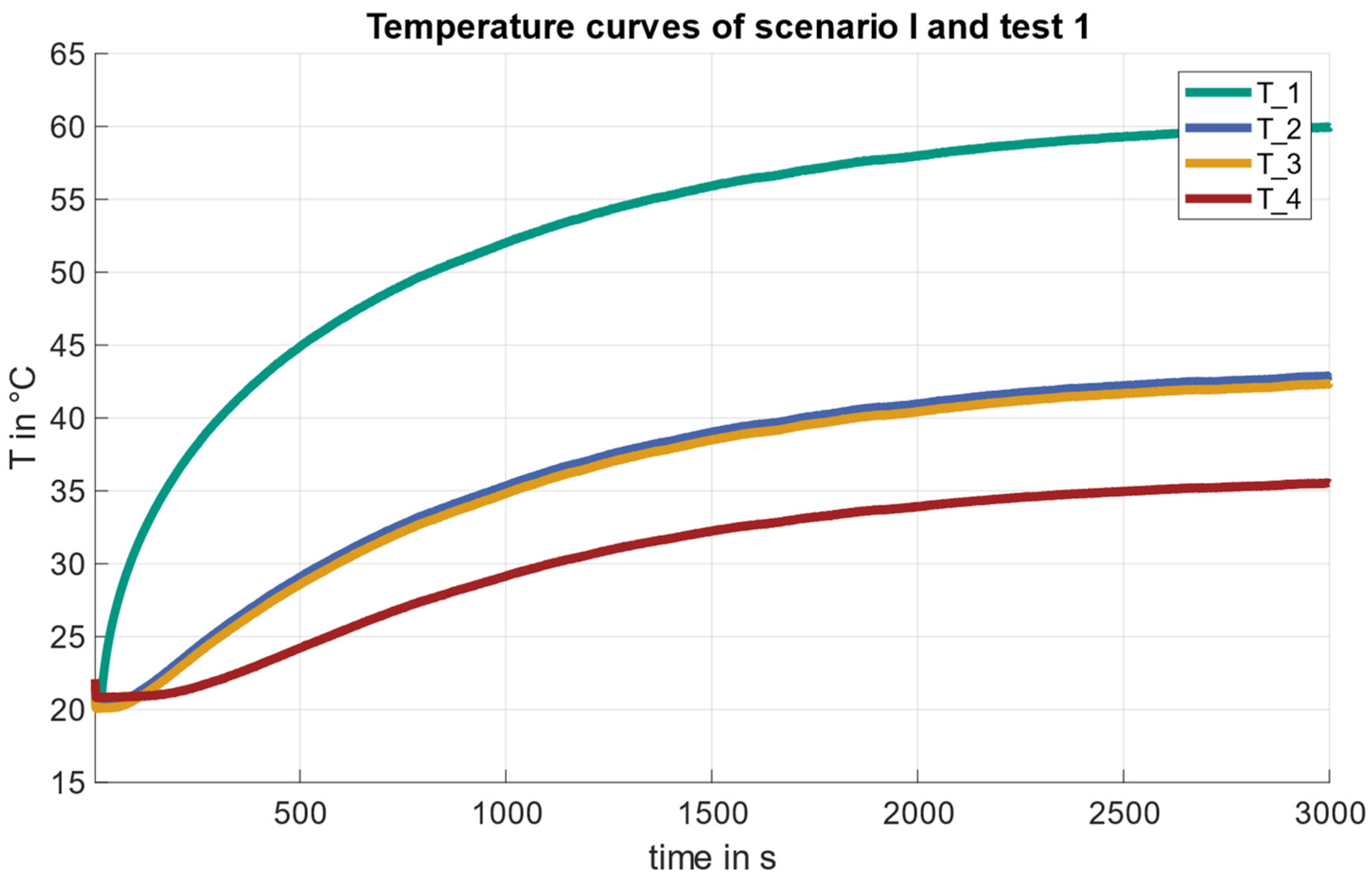
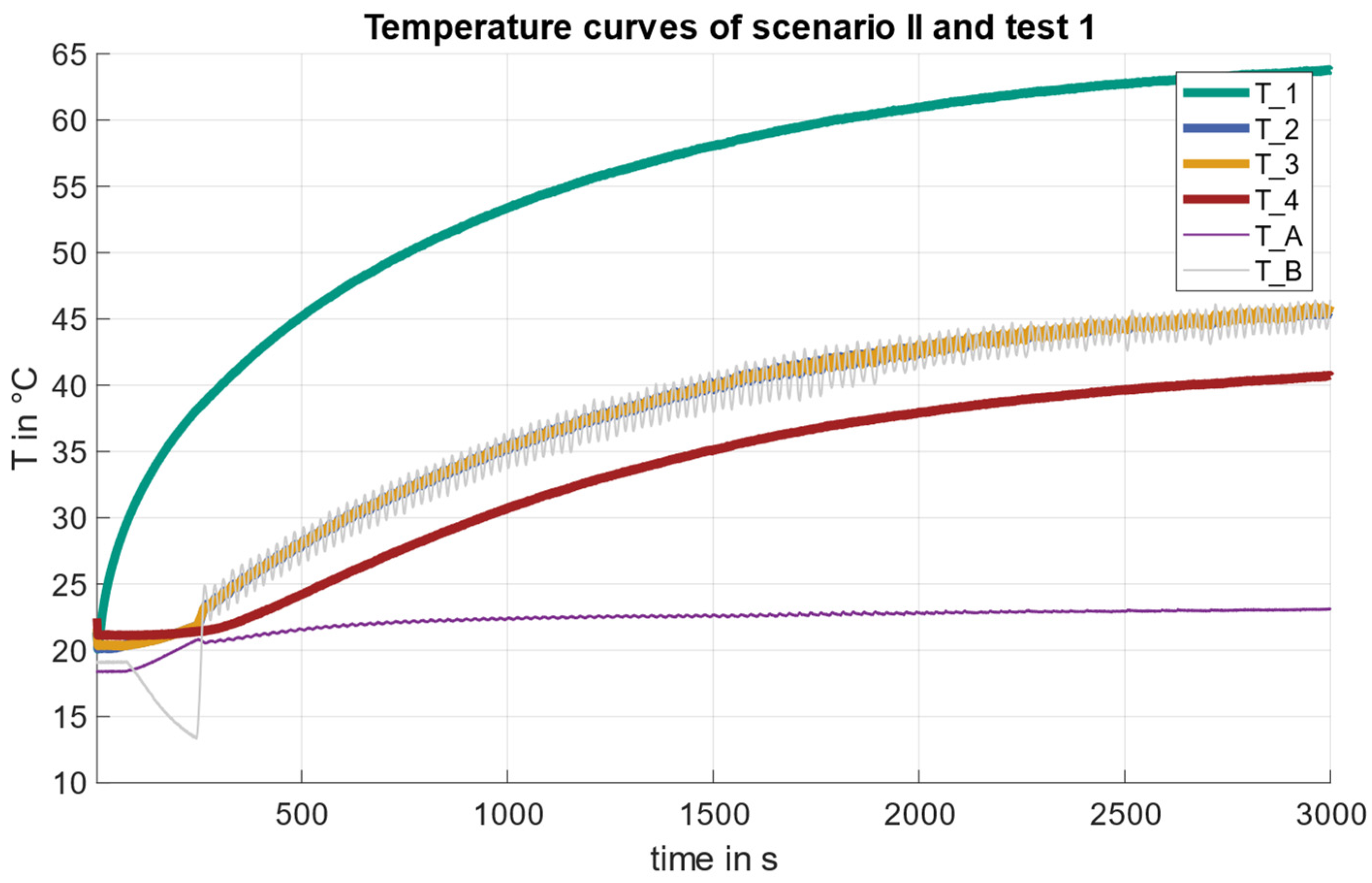
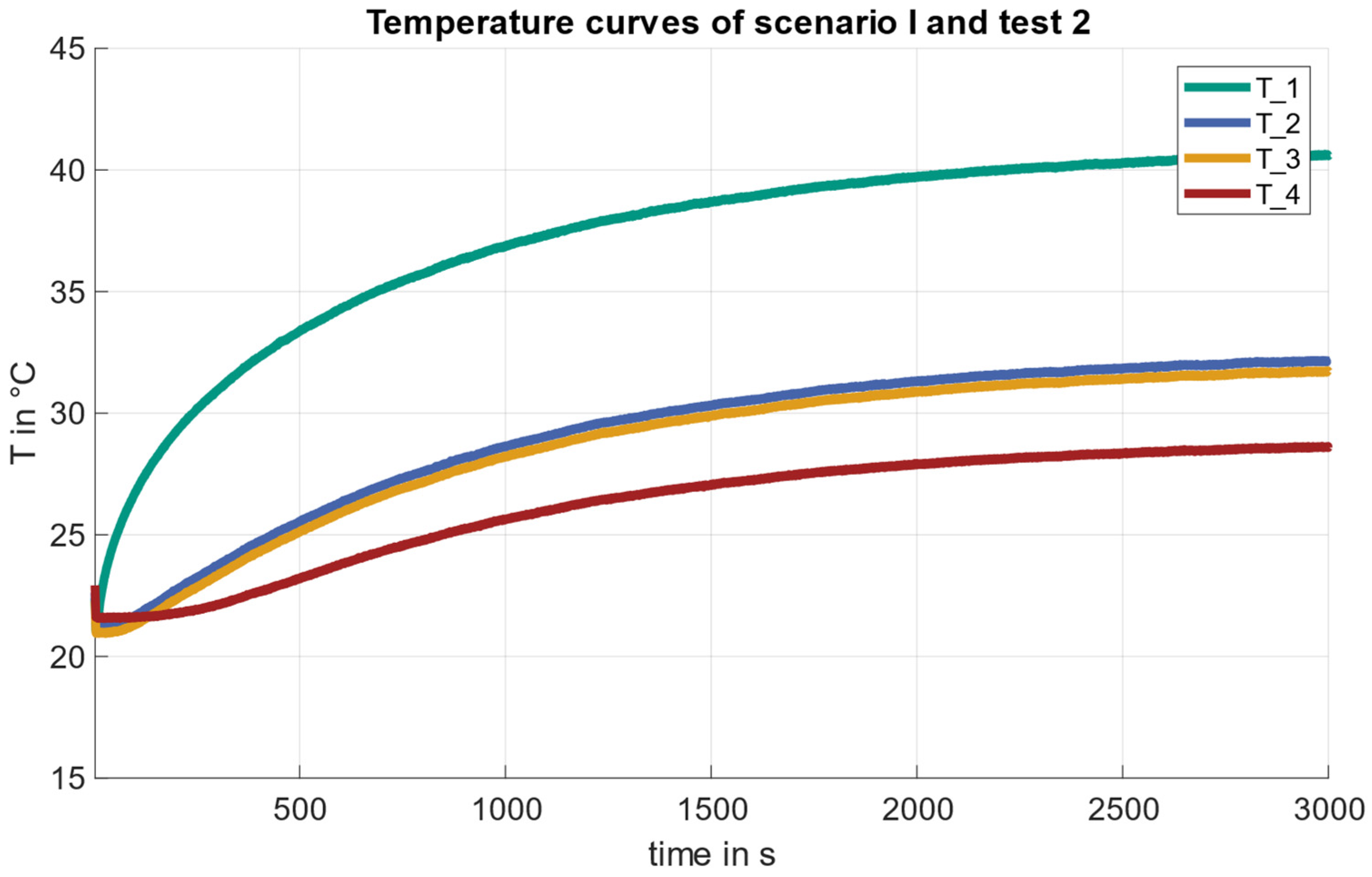
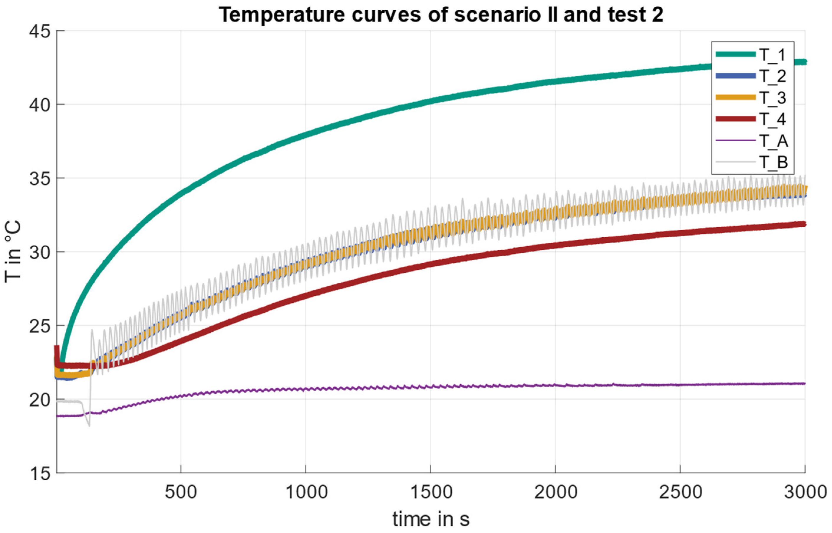
The temperature curves of sensor 1, 2, 3, and 4 of the first test case with a heat flux of 100 W for both scenarios are shown in Figure 6 and Figure 7.

Figure 6. Temperature profiles of the test case 1 (${\dot{Q}}_A=100 \mathrm{W})$ compared for scenarios (I).

Figure 7. Temperature profiles of the test case 1 (${\dot{Q}}_A=100 \mathrm{W})$ compared for scenarios (II).

In scenario I (assembled subsystems), the observed temperature profiles exhibit a predictable pattern. The temperatures reach nearly steady state. Sensors 2 and 3 consistently maintain a maximum temperature difference of 1 °C. This phenomenon can be attributed to the influence of contact resistance, which arises from the thermal impedance at the interface between the two subsystems. As thermal energy is conducted from sensor 1 to sensor 4, the convective and radiative heat transfer mechanisms diminish the overall heat flow along the thermal conduction path. When heat is applied at sensor 1, it takes some time for the thermal energy to propagate through the medium and reach the neighboring positions. This delay is caused by the relatively slow process of thermal conduction. As a result, sensors 2, 3, and 4 experience a gradual increase in temperature.

In scenario II (spatially separated subsystems with TCS), the observed temperature profiles follow the same characteristics. After approximately 300 s, a deviation can be observed in the temperature curves. This behavior is attributed to the system’s control, where it actively intervenes in the system. The temperature curves of measurement points 2 and 3 overlap closely. In addition, both start to oscillate slightly by around 0.5 °C. It is noticeable that the temperature continues to rise rather than reaching a steady-state final temperature compared to scenario I. T_A and T_B are the temperature sensors on the respective Peltier devices on the opposite side of the subsystems. Side A of the TCS is cooled by the fan and remains at a constant temperature after a slight increase of $1 °\mathrm{C}$. Side B of the TCS is heated by a two-point control. T_B thus follows the temperature curve of measuring point 3 and also oscillates with the same frequency, but with an amplitude of approx. 1.5 °C.

The temperatures after 3000 s can be used as an evaluation variable. Table 2 shows these with the associated deviations between the two scenarios. The use of the TCS shows a higher temperature at all temperature measuring points. This is between 2.9 and 5.2 °C depending on the temperature measuring point.

Table 2. Temperatures of test case 1 $\left({\dot{Q}}_A=100 \mathrm{W}\right)$ after 3000 s.

Temperature Sensor	Scenario (I)	Scenario (II)	Deviations
1	60.0 °C	64.0 °C	+4.0 °C
2	43.0 °C	45.9 °C	+2.9 °C
3	42.3 °C	45.8 °C	+3.5 °C
4	35.7 °C	40.9 °C	+5.2 °C

4.2. Test Case 2: 50 W

The temperature curves of sensor 1, 2, 3, and 4 of the first test case with a heat flux of 50 W for both scenarios are shown in Figure 8 and Figure 9.

Figure 8. Temperature profiles of test case 2 (${\dot{Q}}_A=50 \mathrm{W})$ compared for scenarios (I).

Figure 9. Temperature profiles of test case 2 (${\dot{Q}}_A=50 \mathrm{W})$ compared for scenarios (II).

In scenario I (assembled subsystems), the observed temperature still exhibits a predictable pattern, but with lower temperature values compared to test case 1 due to the lower heat flux.

In scenario II (spatially separated subsystems with TCS), there is the same behavior as in test case 1. After 200 s, there is a deviation caused by the control. After that, the temperatures of sensors 2 and 3 overlap closely. The effect of oscillating temperatures T_2, T_3, and T_B also occurs.

Table 3 shows the temperatures with the associated deviations between the two scenarios after 3000 s. The use of the TCS shows a higher temperature at all temperature measuring points. This is between 1.8 and 3.4 °C depending on the temperature measuring point. It shows that subsystem B is, in general, hotter in scenario (II) compared to scenario (I).

Table 3. Temperatures of test case 2 $\left({\dot{Q}}_A=50 \mathrm{W}\right)$ after 3000 s.

Temperature Sensor	Scenario (I)	Scenario (II)	Deviations
1	40.6 °C	43.0 °C	+2.4 °C
2	32.2 °C	34.0 °C	+1.8 °C
3	31.8 °C	34.3 °C	+2.5 °C
4	28.6 °C	32.0 °C	+3.4 °C

5. Discussion

This chapter will discuss the results of an experimental study. The aim is to validate whether the TCS described in Section 3.2 can be utilized to answer the research question, which is, “How can thermal interactions by heat conduction be transferred between spatially separated physical subsystems in order to perform an early assessment of functional system reliability?”. Additionally, the chapter will elaborate on the limitations and suggest further research directions.

5.1. Discussion of the Experimental Study

One significant finding of the study is that the variations in temperatures can be deemed acceptable. Consequently, absolute values of temperature deviations may vary significantly across different test cases. Notably, test case 1 exhibits larger deviations compared to test case 2, indicating that the heat flow magnitude plays a crucial role in influencing these variations. The observed trend of larger deviations in test case 1, associated with higher heat flows, suggests a direct correlation between heat flow magnitude and temperature deviations. As heat flows increase, so do the variations in stationary end temperatures. This trend highlights the importance of understanding and accounting for heat flow effects during thermal analysis and system design. Despite the presence of more considerable absolute deviations in higher heat flow scenarios, the relative deviations remain relatively stable.

All deviations are positive; therefore, it can be stated that using the TCS leads to higher temperatures. When a Peltier device experiences a temperature difference between its two sides, heat conduction generates an opposing heat flow (see Equations (6) and (7)). It is possible that the backward heat flow within the TCS is greater than expected based on the model of the open-loop control. Because the thermal coupling condition keeps the temperature difference between temperature sensors 2 and 3 at zero (see Equation (3)), subsystem B is also heated more, which results in a temperature increase. In addition, on side B of the TCS, the cooling side of the Peltier device is heated. This is to prevent the temperature differences between the two sides of the Peltier device from becoming too great. Only a two-point control is implemented at this point. The control deviation can result in a slightly increased heat input. This explains why all four temperature sensors on the subsystems are higher. We do not have a hypothesis as to why the deviations are not the same for all four temperature sensors. However, the differences between the individual sensors are below the tolerance of ±1.5 °C (thermocouple, type J, class 1).

The observed deviations in temperatures have practical implications for assessing the thermal damage limit of the system. Understanding the range of temperature variations under different heat flow conditions helps establish safe operational limits and ensures the system’s longevity and reliability. In this context, it is crucial to consider the effects of the TCS, which may introduce additional deviations but serves as a conservative approach in testing.

Another important aspect is to discuss is the TCS in testing to assess of temperature-dependent performance. The small magnitude of the observed deviations, typically remaining within a low single-digit percentage range, indicates that the temperature effects on system performance are minimal under the test conditions. Significant impacts on temperature-sensitive parameters of components like hydraulic oil or electric motors only become evident when exposed to substantial temperature differences.

Despite the absolute deviations introduced by the TCS, it offers a valuable advantage in the investigation of system reliability. By enabling the creation of qualitative temperature trends, the TCS allows for a holistic assessment of the system’s thermal behavior. Spatially separated subsystems without the TCS would generate entirely different temperature profiles, limiting the ability to identify potential weaknesses in the system’s thermal management. Hence, the thermal coupling system proves to be instrumental in understanding and improving the overall thermal performance and reliability of the system.

5.2. Limitations

An essential aspect highlighted by the study is to improve the control system to avoid the deviations that occurred. A well-designed control system can help maintain temperatures within tighter tolerances and reducing absolute deviations. The TCS applied in this test case has a deviation of maximum 5.2 °C. For some applications this is required to be lower. Efforts should be made to optimize the control using appropriate data-driven methods.

The contact resistance between the spatially separated subsystems in a thermal coupling system must be thoroughly examined. To improve the accuracy of the thermal coupling system, further investigation is required to understand the impact of contact resistance in the deviations from the experiments shown. By incorporating the contact-resistance calculations and compensation techniques into the control system, it is possible to account for deviations caused by changes in the interface properties and maintain the thermal coupling condition.

An additional limitation is the accuracy of the used temperature sensors. It is ±1.5 °C for the temperature range used. The temperature deviations caused by this can be seen at beginning of the tests. All temperature sensors should have the same value. However, the deviations are up to 3 °C and are, therefore, just within the accuracy. As the sensors were kept the same between scenarios (I) and (II), this has no effect on the study results themselves. However, it should be taken into account if such a coupling system is used and a statement is to be made about the thermal damage limit.

5.3. Further Research Directions

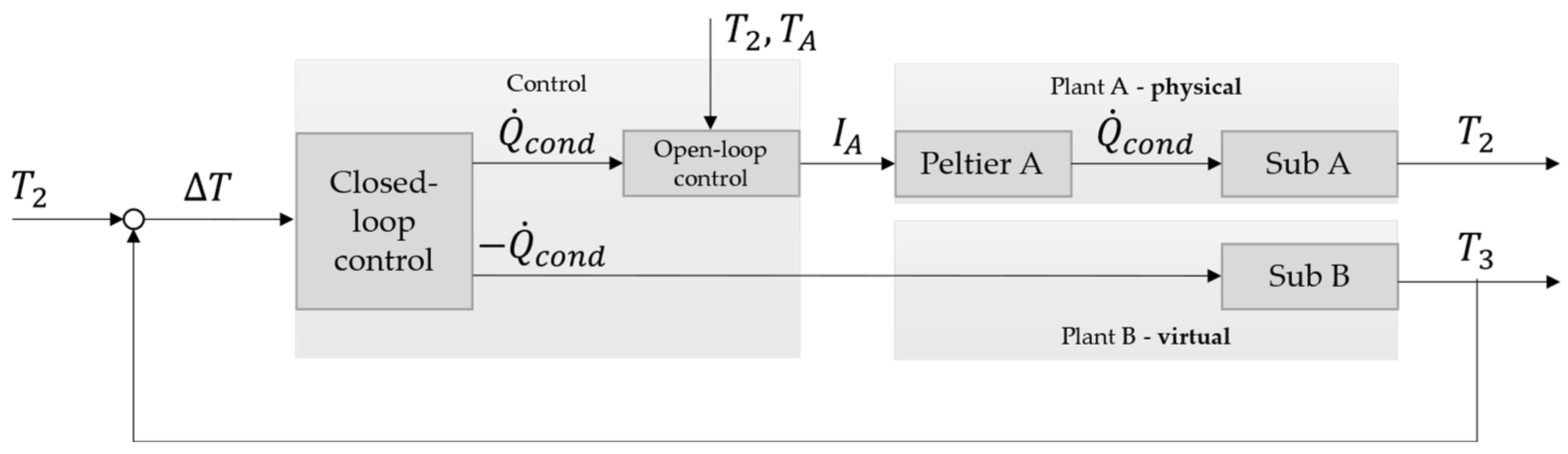
The potential of the described thermal coupling system goes beyond merely connecting two spatially separated physical subsystems. It can be expanded to transfer thermal interactions between physical components and virtual simulations, opening up new possibilities for testing and analysis, especially in the context of XiL test benches. One of the main advantages of coupling physical and virtual components is the ability to conduct experiments that might otherwise be impractical, expensive, or even dangerous in a purely physical setup. By simulating certain subsystems, engineers can save time and resources while still obtaining meaningful results. By considering the thermal interactions, a prediction can be made about the thermal damage limit and the temperature-dependent performance.

Figure 10 shows the changed concept for physical–virtual coupling. The open-loop control can be omitted, because, in the simulation, the heat flow can be used directly. A compensation through the influence of the Peltier devices is not needed. However, this adjusted control system still needs to be implemented and validated.

Figure 10. Control system of the thermal coupling system to consider thermal interactions between physical and virtual subsystems.

Since the thermal coupling system can be validated in that way, it must now be applied to a system. It is planned to use it on an aerospace actuator, more precisely on an electrohydrostatic actuator (EHA). An EHA is a type of actuator commonly used in aircraft control systems, such as flaps and slats, and it combines the advantages of both hydraulic and electric actuation systems. Currently, these systems demonstrate limited reliability for long-term operations due to thermal damage, and are thus primarily utilized for short-term, secondary flight-control system applications. However, for efficiency and sustainability, it is crucial to employ them as primary control systems. To facilitate reliable testing, it is essential to simulate realistic conditions on the ground. This involves considering interactions with surrounding systems such as power units, wings, etc. While mechanical interactions can be effectively replicated using state-of-the-art test benches (e.g., [36]), the replication of thermal interactions remains a challenge. The TCS is designed to bridge this gap, enabling the transfer of thermal interactions between the power unit and the EHA. The objective extends beyond merely assessing the thermal damage limit; it encompasses evaluating the impact of temperature-dependent parameters on the EHA’s accuracy and efficiency, particularly emphasizing the latter. This comprehensive approach aims to enhance the overall reliability and performance of the system in long-term operational scenarios. The environmental tests of the DO-160 are to be used for this [11].

6. Conclusions

The study confirmed that the thermal coupling system (TCS) consisting of Peltier devices and a control system based on a combination of closed-loop and open-loop control can be used to transfer thermal interactions between spatially separated physical subsystems. The experimental study demonstrated that the TCS produced deviations within a range of max. 5.2 °C in the tests carried out. The measuring accuracy of the temperature sensors themselves is ±1.5 °C. Higher heat flows lead to larger deviations, suggesting a correlation between heat flow magnitude and temperature deviations. All observed deviations are positive, indicating that using the TCS leads to higher temperatures. This could be due to the opposing heat flow generated by heat conduction in the Peltier device. The temperature deviations of the TCS are within a range where it can be used in testing to assess the temperature-dependent performance of systems and the thermal damage limit.

However, it is important to acknowledge the limitations of our study, including temperature deviations. To enhance the TCS’s precision, additional research should be devoted to understanding contact resistance and implementing compensation techniques in the control system. In-depth exploration of these factors could lead to significant improvements in the system’s accuracy and efficiency. Further test cases should be used for this purpose. Additionally, the TCS should be expanded to transfer thermal interactions between physical components and virtual simulations. This needs to be tested in a concrete application scenario. Our plan is to transfer the thermal interactions between a virtual power unit and a physical electrohydrostatic actuator used in the aerospace industry. The influence of temperature on system performance is to be investigated.

The TCS contributes to a better understanding of thermal interactions in complex systems and provides a valuable tool for enhancing overall system reliability through thermal testing and validation.