Impact of the Regulation Strategy on the Transient Behavior of a Brayton Heat Pump

Abstract

High-temperature heat pumps are a key technology for enabling the complete integration of renewables into the power grid. Although these systems may come with several variants, Brayton heat pumps are gaining more and more interest because of the higher heat sink temperatures and the potential to leverage already existing components in the industry. Because these systems utilize renewable electricity to supply high-temperature heat, they are particularly suited for industry or energy storage applications, thus prompting the development of various demonstration plants to evaluate their performance and flexibility. Adapting to varying load conditions and swiftly responding to load adjustments represent crucial aspects for advancing such systems. In this context, this study delves into assessing the transient capabilities of Brayton heat pumps during thermal load management. A transient model of an emerging prototype is presented, comprising thermal and volume dynamics of the components. Furthermore, two reference scenarios are examined to assess the transient performance of the system, namely a thermal load alteration due to an abrupt change in the desired heat sink temperature and, secondly, to a sudden variation in the sink mass flow rate. Finally, two control methodologies—motor/compressor speed variation and fluid inventory control—are analyzed in the latter scenario, and a comparative analysis of their effectiveness is discussed. Results indicate that varying the compressor speed allows for a response time in the 8–20 min range for heat sink temperature regulation (first scenario). However, the regulation time is conditioned by the maximum thermal stress sustained by the heat exchangers. In the latter scenario, regulating the compressor speed shows a faster response time than the inventory control (2–5 min vs. 15 min). However, the inventory approach provides higher COPs in part-load conditions and better stability during the transient phase.

1. Introduction

1.1. Background

The latest report from the International Energy Agency [1] underscores heat production as the most significant contributor to global energy usage, constituting nearly half of the world’s final energy consumption. In 2021, the industrial sector accounted for approximately 51% of energy consumption for heat production, with domestic use, including heating buildings and water, representing 46%, and agricultural activities utilizing 3%. As non-renewable energy sources still satisfy more than 60% of heating energy demand [1], decarbonizing heat production is crucial to achieving carbon neutrality.

Over the past years, high-temperature heat pumps have emerged as a pivotal technology while addressing the need to reduce carbon emissions associated with heating [2]. Notably, these systems can harness surplus renewable energy to transfer heat from low-temperature sources to high-temperature heat utilizers. To date, a variety of heat pump models are commercially available, from absorption and vapor compression to rotational, hybrid, and transcritical heat pumps [3,4]. In their review study, Arpagaus et al. [5] highlighted that the majority of industrial heat pumps on the market can supply heat to 90 °C, with only a minority capable of reaching temperatures in the range of 140–160 °C. Beyond domestic applications, these systems primarily find use in industries requiring low-temperature heat. Nonetheless, several works have demonstrated that different European industries require high-temperature heat [6,7], and heat pumps could partly cover such demand if sink temperatures above 100 °C could be reached. For instance, process heat could be used for steam generation, and heat pumps could be effectively employed in case of heat sink temperatures above 130 °C [8].

The advancement of heat pump technology faces challenges such as low efficiency, high equipment costs, extended payback periods, limitations of components, and a need for environmentally friendly operating fluids suitable for high temperatures [9]. While the Rankine thermodynamic cycle underpins most common models, alternatives based on the Brayton cycle may offer higher performance depending on the temperature glides of the heat sources and sinks [4]. Zühlsdorf et al. [10] suggested that technically and economically feasible heat pumps capable of supplying heat up to 280 °C could be developed by leveraging equipment already available in the oil and gas industry. Under this approach, various concepts aiming to supply heat at temperatures higher than 150 °C have been put forward in the literature for industrial and energy storage applications [5,11]. However, these systems need to be developed, realized, and integrated into relevant industries. Moreover, these systems should offer grid flexibility by enabling rapid start-ups or accommodating quick load variations while maintaining high efficiencies for optimal performance.

Despite flexibility being a crucial aspect for demonstrating such technology, only a limited number of studies have delved into the transient performance of industrial Brayton heat pumps, primarily focusing on the cold start-up of the system [12,13]. In particular, Ferrari et al. [13] reported a start-up time of approximately two hours and found the maximum thermal stresses sustained by the heat exchangers to be the primary limitation for a fast maneuver. However, the work did not analyze the system behavior during thermal load regulation.

1.2. Objectives and Elements of Novelty

This paper aims to assess the transient capabilities of a novel Brayton heat pump during thermal load regulation. Preliminary results on this topic have been reported in Ref. [14]. In this study, a more extended analysis is proposed, with particular reference to the following scenarios:

• A thermal load alteration caused by an abrupt change in the desired heat sink temperature;
• A thermal load alteration due to a sudden variation in the sink mass flow rate. In the former scenario, the motor/compressor speed adapts to the heat sink temperature at the desired setpoint.

In the latter, two distinct control methodologies—motor/compressor speed variation and fluid inventory control—are employed to maintain the heat sink temperature, allowing for a comparative analysis of their effectiveness.

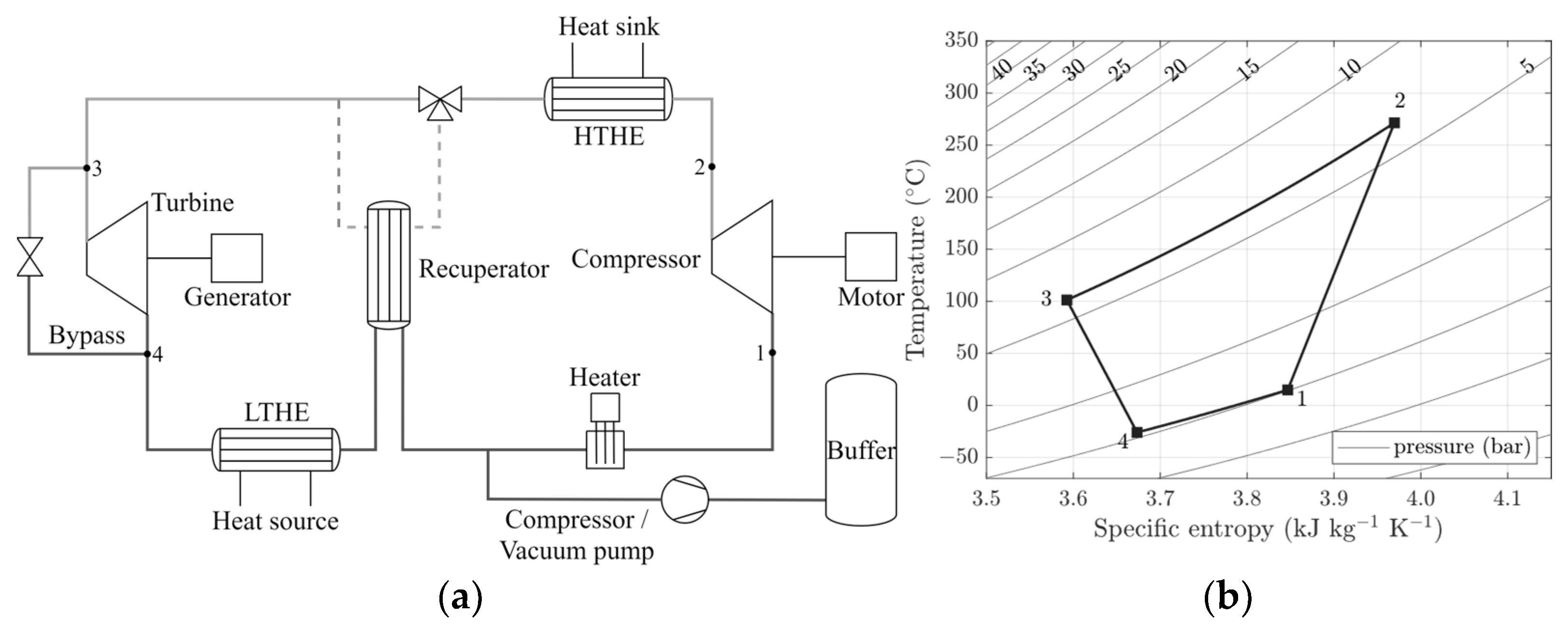
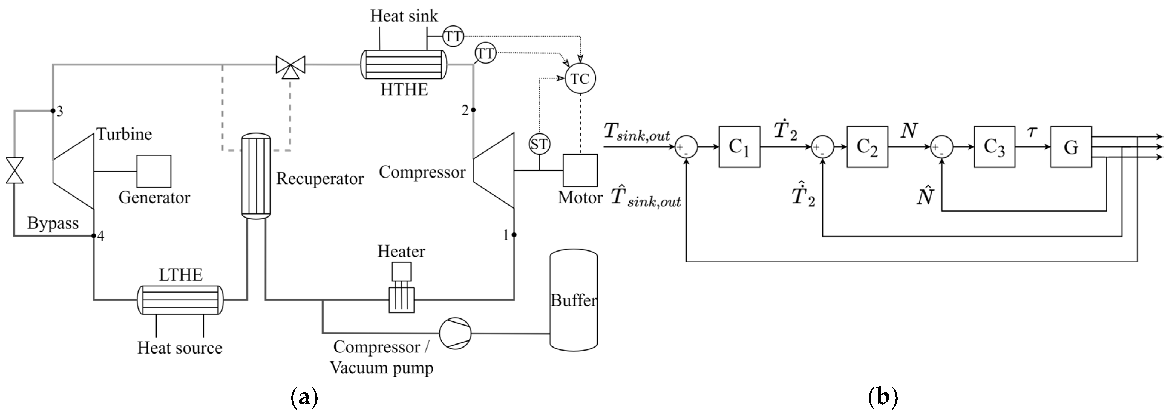
2. Case Study

The present study examines the Brayton heat pump recently developed by the German Aerospace Center (DLR) in Cottbus, Germany [12].

As depicted in Figure 1a, the prototype features a two-stage axial turbine, a three-stage turbocompressor, and three shell-and-tube heat exchangers. The system operates according to the reversed-Brayton cycle, which is reported in Figure 1b. Therefore, the compressor initially elevates the temperature and pressure of a designated operating fluid (e.g., dry air, Argon, or CO₂) using electrical power (line 1–2). Subsequently, the high-temperature heat exchanger (HTHE) transfers heat to the thermal user (line 2–3), after which the gas expands through the turbine, recovering power and lowering its temperature below 0 °C (line 3–4). A low-temperature heat exchanger (LTHE) enables heat transfer between a source at a low temperature and the gas contained in the closed cycle, which then returns to the compressor (line 4–1). Additionally, the system comprises a recuperator designed for internal heat recovery, as well as a heater capable of raising the fluid’s temperature at the compressor inlet when needed.

For the purposes of this study, the recuperator is assumed inactive despite being part of the actual plant layout. In this configuration, the system supplies 115 kW of sensible heat in the range of 272−100 °C with a coefficient of performance (COP) of approximately 1.3. The system operating conditions are reported in

Table 1. System operating conditions (non-recuperated layout).

Description	Point	T (°C)	p (bar)	$\dot{\mathit{m}}$ (kg s−1)
Cycle	1	15.00	1.013	0.658
	2	271.40	6.282	0.658
	3	101.30	6.128	0.658
	4	−25.85	1.085	0.658
Sink	inlet	15.00	1.08	0.458
	outlet	261.40	1.017	0.458
Source	inlet	17.20	1.239	1.011
	outlet	−9.46	1.067	1.011

. On the other hand, it is worth noting that the system operates as a closed cycle, enabling fluid inventory control to adjust the sink thermal load by adding or extracting mass into/from the system from a secondary circuit. In this work, the inventory circuit is simplified by considering an ideal apparatus capable of moving mass from the heat pump to the buffer (or environment) and vice versa.

3. Methods

A physical model of the plant comprehensive of control systems was developed using Simulink^® and Simscape^™ libraries in Matlab^® R2022b (9.13.0.2049777) [15]. Moreover, dry air was assumed in both sink, source, and closed circuit. RefProp [16] was employed to compute its thermophysical properties.

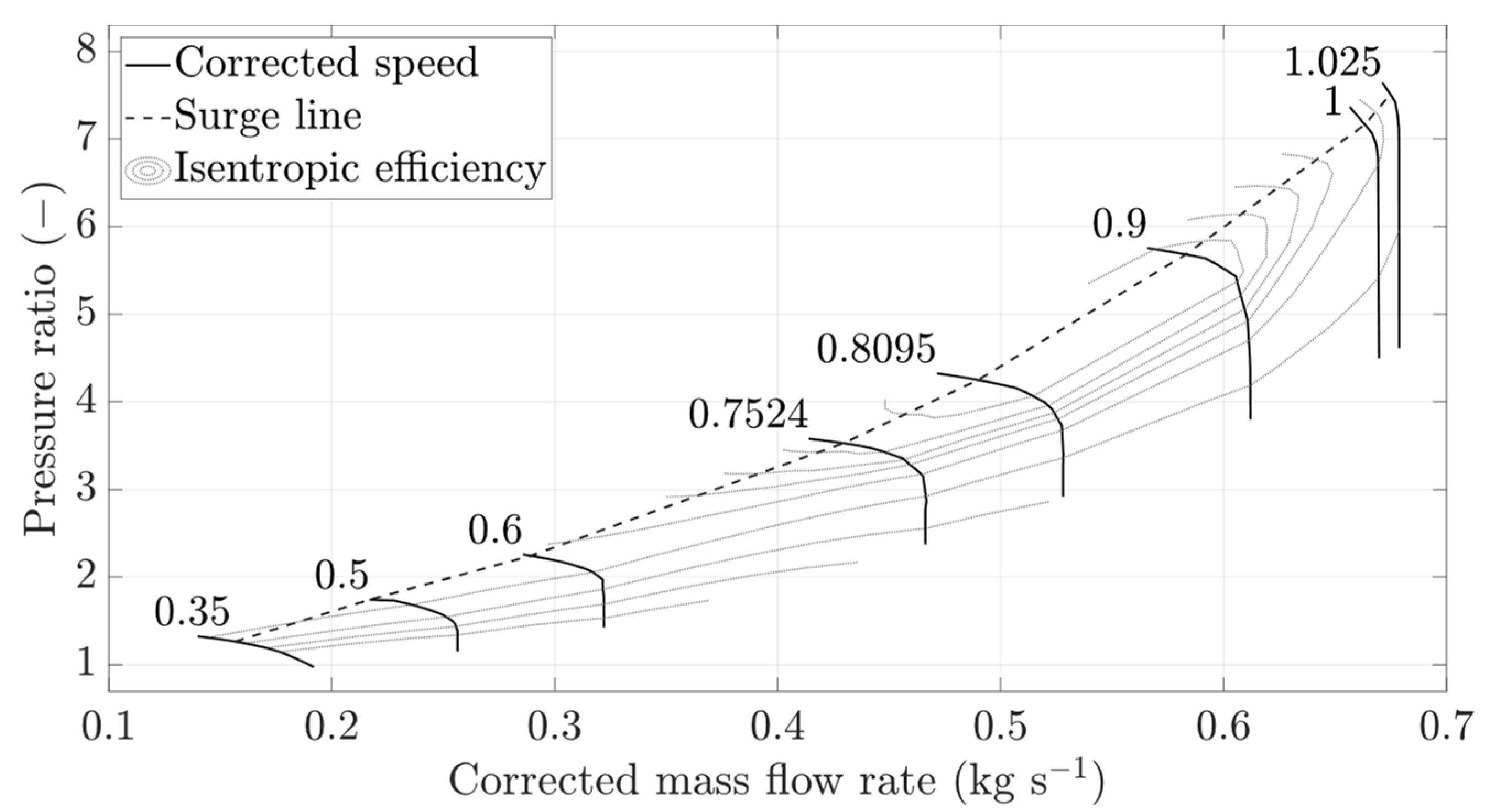
3.1. Turbomachinery

Turbomachines were considered adiabatic and did not contribute to the total gas volume of the system. Therefore, mass and energy were conserved, as in Equations (1) and (2):

$${\dot{m}}_{in}+ {\dot{m}}_{out}= 0,$$

(1)

$${\dot{\Phi }}_{in}+{\dot{\Phi }}_{out}+{\dot{W}}_{fluid}=0,$$

(2)

where ${\dot{m}}_i$ and ${\dot{\Phi }}_{in}$ are the mass and energy flow rates at the machine inlet/outlet and ${\dot{W}}_{fluid}$ is the fluid thermodynamic power computed as:

$${\dot{W}}_{fluid}=\left\{\begin{array}{c}{-\dot{m}}_{in}{\eta }_{is}{\Delta h}_{is}, if turbine\hfill \\ {\dot{m}}_{in}\frac{{\Delta h}_{is}}{{\eta }_{is}},\hspace{0.33em}\hspace{0.33em}\hspace{0.33em}\hspace{0.33em}\hspace{0.33em}if compressor\end{array}\right.$$

(3)

where ${\Delta h}_{is}$ and ${\eta }_{is}$ are the isentropic enthalpy drop and efficiency, respectively. Finally, the power recovered through the turbine or adsorbed by the compressor was determined using Equations (4) and (5):

$${\dot{W}}_{turb}={{\eta }_m\dot{W}}_{fluid},$$

(4)

$${\dot{W}}_{comp}={\dot{W}}_{fluid}/{\eta }_m,$$

(5)

where ${\eta }_m$ is the mechanical efficiency of the turbomachine. Thermal dynamics related to turbomachinery were disregarded. On the other hand, the model accounted for the moment of inertia of the turbomachines, transmission, motor, and generator. Hence, inertial torques were determined as in Equation (6):

$$\tau =J\frac{dN}{dt},$$

(6)

where $J$ is the moment of inertia of the specific component and $N$ is its rotational speed. Performance maps from DLR were utilized to define the off-design characteristics of the turbomachines. Figure 2 reports the compressor map used in the present work, expressed as a function of corrected parameters defined according to Equation (7):

$$\left\{\begin{array}{c}{\dot{m}}_{corr}= {\dot{m}}_{in}\frac{\sqrt{T_{in}/T_{ref}}}{p_{in}/p_{ref}}\\ N_{corr}=\frac{N}{\sqrt{T_{in}/T_{ref}}}\end{array}\right.,$$

(7)

where $p_{ref}= 101,325$ Pa, $T_{ref}=$288.15 K, $N$ is the rotational speed, and ${\dot{m}}_{in}$, $T_{in}$, $p_{in}$ are the mass flow, temperature, and pressure at the machine inlet.

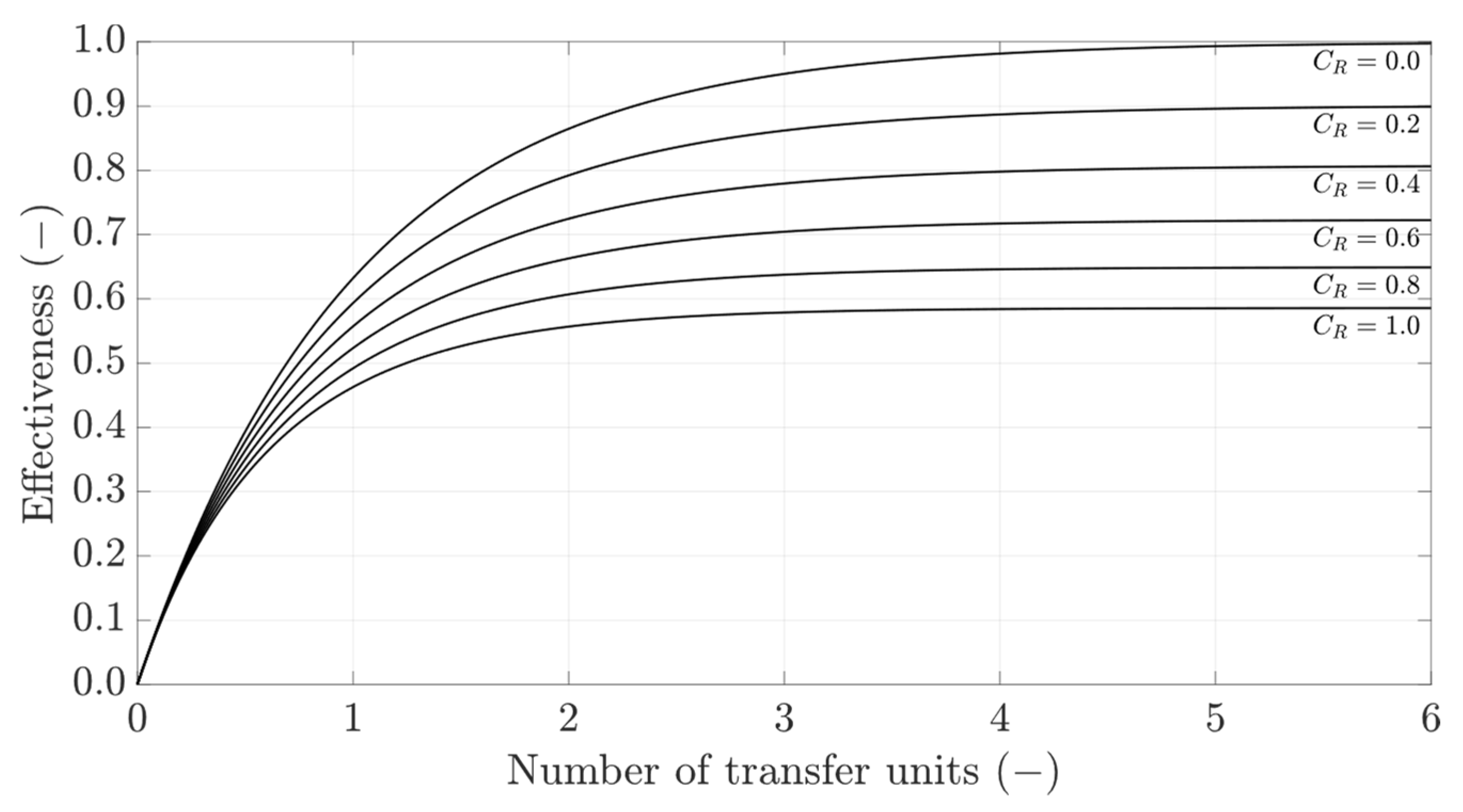
3.2. Heat Exchangers

Three countercurrent shell-and-tube heat exchangers were considered in the model. Technical data provided by the producer were employed to set up the designated components within the Simscape™ Fluids library [17]. The flows on either side of the heat exchanger were established using the mass and energy balances detailed in Equations (8) and (9):

$$\left[\left({\left(\frac{\partial \rho }{\partial p}\right)}_u\frac{d{p}_I}{dt}+\right.{\left(\frac{\partial \rho }{\partial u}\right)}_p\frac{du}{dt}\right]V={\dot{m}}_{in}+{\dot{m}}_{out},$$

(8)

$$\left[\left({\left(\frac{\partial U}{\partial p}\right)}_{T,V}\frac{d{p}_I}{dt}+\right.{\left(\frac{\partial U}{\partial T}\right)}_{p,V}\frac{d{T}_I}{dt}\right]={\dot{\Phi }}_{in}+{\dot{\Phi }}_{out}+\dot{Q},$$

(9)

where $\dot{Q}$ is the exchanged heat flow rate, ${\dot{m}}_i$ and ${\dot{\Phi }}_i$ are the mass and energy flow rates at the tube or shell inlet/outlet, and $p_I$, $T_I$, $\rho$, $V$, $U$ are the gas pressure, temperature, density, volume, and internal energy. As for the pressure drop, they were modeled according to Equation (10):

$$\frac{∆p }{\mathsf{\Delta }{p}_{nom}}= \left(\frac{{\rho }_{nom}}{\rho }\right){\left(\frac{\dot{m}}{{\dot{m}}_{nom}}\right)}^2.$$

(10)

Furthermore, the heat flow rate transferred through the heat exchanger was determined based on the ε-NTU method [18], summarized in Equation (11):

$$\left\{\begin{array}{c}\dot{Q}=\epsilon \cdot C_{min}\cdot \left(T_{hot,in}-T_{cold,in}\right)\\ NTU=\frac{1}{C_{min}{R}_{overall}} \\ \epsilon = f\left(NTU,C_r\right) \end{array}\right.,$$

(11)

where $\dot{Q}$ denotes the heat flow rate, ε is the effectiveness, $C_{min}$ is the minimum thermal capacity rate, $C_r=C_{min}/C_{max}$ is the thermal capacity ratio, and $R_{overall}$ represents the overall thermal resistance of the heat exchanger. Figure 3 reports the ε-NTU correlation used in the present study.

The metal mass of the heat exchangers was included in the model, thus accounting for their thermal inertia. In particular, the heat exchange between the tube and shell was determined according to:

$${\dot{Q}}_{tube}=\dot{Q}+C_{wall,tube}{\dot{T}}_{wall,tube},$$

(12)

$${\dot{Q}}_{shell}=\dot{Q}-C_{wall,shell}{\dot{T}}_{wall,shell},$$

(13)

where $C_{wall,i}$ and ${\dot{T}}_{wall,i}$ are the thermal capacity and temperature rate of the tube/shell side and $\dot{Q}$ is the heat transfer rate computed according to Equation (11).

3.3. Piping and Valves

The model accounted for the gas volume and thermal inertia due to the piping. To this end, the gas volume and metal mass of each pipe were determined based on the pipe’s actual geometry. As for the mathematical model of the pipes, mass and energy were conserved analogously to the heat exchangers through Equations (8) and (9). Conversely, pressure drops were computed as:

$$p_i-p_I={\left(\frac{{\dot{m}}_i}{S}\right)}^2\left(\frac{1}{{\rho }_i}-\frac{1}{{\rho }_I}\right)+{∆p}_{iI},$$

(14)

where ${∆p}_{iI}$ are the pressure losses due to viscous friction, $S$ is the pipe’s cross-sectional area, and the subscripts $I$ and $i$ denote the physical quantities of the gas volume at the pipe’s inlet/outlet, respectively. Finally, the heat transferred through the pipe was determined according to Equations (15)–(17):

$$\dot{Q}={\dot{Q}}_{conv}+{\dot{Q}}_{cond},$$

(15)

$${\dot{Q}}_{conv}=\left|{\dot{m}}_{avg}\right|c_{p,avg}\left(1-exp(-\frac{{\alpha }_{avg}A}{\left|{\dot{m}}_{avg}\right|c_{p,avg}})\right)\left(T_{wall}-T_{in}\right)+\frac{k_{I}A}{d_h}\left(T_{wall}-T_i\right),$$

(16)

$${\dot{Q}}_{cond}=2\pi k_{mat}L\left[\frac{\left(T_{mat}-T_{in}\right)}{\mathit{ln}\left(\frac{d_{avg}}{d_{in}}\right)}+\frac{\left(T_{out}-T_{mat}\right)}{\mathit{ln}\left(\frac{d_{out}}{d_{avg}}\right)}\right]+c_{mat}{M}_{mat}{\dot{T}}_{mat}.$$

(17)

In more detail, Equation (16) models the heat exchanged between the fluid and the pipe wall, while Equation (17) describes the pipe’s thermal mass effects as well as the heat transfer due to conduction through the pipe material. Further details concerning the mathematical model of the pipe are provided in [17,19].

For what concerns the turbine bypass, it was modeled as an adiabatic variable size orifice with negligible gas volume. The mass flow through the valve was determined based on the flow conditions according to Equation (18):

$$\dot{m}=\left\{\begin{array}{c}{C}_v{\xi }_6\left(1-\frac{1-{PR}_{lam}}{3F_{\gamma }{x}_T}\right)\sqrt{\frac{{\rho }_{avg}}{p_{avg}\left(1-{PR}_{lam}\right)}}\left(p_{in}-p_{out}\right) if PR>{PR}_{lam} \\ C_v{\xi }_6\left(1-\frac{p_{in}-p_{out}}{3p_{in}{F}_{\gamma }{x}_T}\right)\sqrt{\left(p_{in}-p_{out}\right){\rho }_{in}} if PR\le {PR}_{lam}\\ \frac{2}{3}{C}_v{\xi }_6\sqrt{F_{\gamma }{x}_T{p}_{in}{\rho }_{in}} if PR<1-F_{\gamma }{x}_T\end{array}\right.,$$

(18)

where $C_v$ is the valve flow coefficient, $p_i$ is the upstream/downstream pressure, ${\rho }_{in}$ is the upstream fluid density, $PR$ is the pressure ratio, $x_T$ is the pressure differential ratio at chocked flow, $F_{\gamma }$ is the ratio of the isentropic exponent, and ${\xi }_6$ is a constant equal to 27.3 for mass flow rate in kg/h, pressure in bar, and density in kg/m³. The valve geometry and its flow characteristic (e.g., the relationship between opening and flow coefficient) were specified based on the manufacturer’s data. Ultimately, the gas volume of the heater was neglected, while its pressure losses were taken into account.

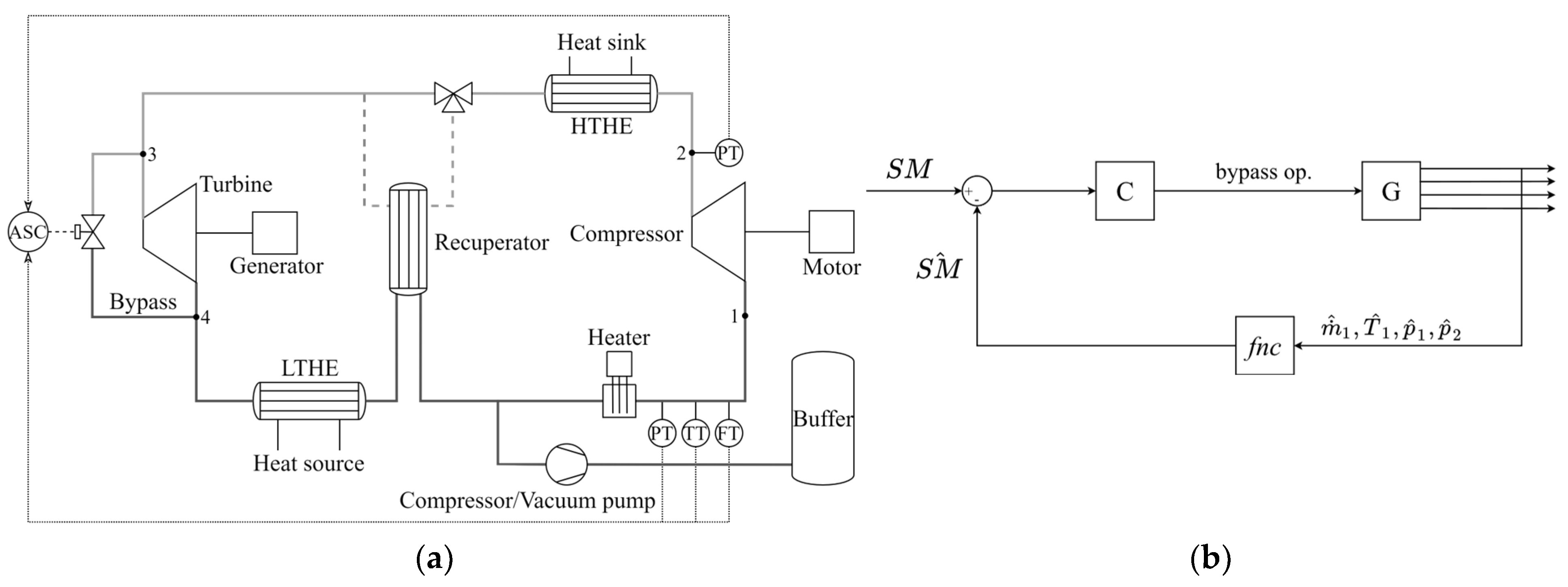
3.4. Control Systems

Several controls were implemented to operate the heat pump, specifically:

• Anti-surge control;
• Temperature/speed control;
• Fluid inventory control.

In this work, a surge margin of at least 10% was ensured via the anti-surge control (ASC), which regulated the turbine bypass to avoid the compressor operating in regions close to the surge line, as shown in Figure 4a.

The bypass opening was determined by means of the control loop outlined in Figure 4b. Therefore, plant measurements were utilized to compute the actual surge margin, defined as:

$$SM ={\left(\frac{P{R}_{surge}}{P{R}_{op}}-1\right)}_{{\dot{m}}_{corr}},$$

(19)

where $P{R}_{op}$ entails the measured pressure ratio and $P{R}_{surge}$ denotes the one on the surge line for an equal corrected mass flow rate. A proportional–integral (PI) controller then computed the bypass opening according to the surge margin residual. Like the other regulators used in the present study, the controller gains were initially derived using the Ziegler–Nichols method and fine-tuned through trial and error. Additionally, due to the saturation of the control actions (e.g., min/max bypass opening), anti-windup techniques were also enabled to help prevent integration wind-up of the regulator.

Conversely, as shown in Figure 5a, the temperature/speed control (TC) allowed the sink temperature to be regulated to a given value by adjusting the motor rotational speed. Only the following control specifications were taken into account, since this study mainly focused on assessing the system response rather than optimizing it:

• Zero residual upon reaching the new steady-state condition;
• Temperature rates below 2 K/min at the compressor outlet [12].

Figure 5. Temperature/speed control: (a) plant schematic; (b) control loop. Points 1 and 2 refer to the compressor inlet and outlet, while points 3 and 4 refer to the turbine inlet and outlet, respectively. The grey and bold lines show the high and low-pressure sides of the plant. The grey dotted line indicates that the recuperator is disabled in the considered plant configuration. Arrows highlight that transducers’ temperature (TT) and rotational speed (ST) measurements are inputs to the TC.

Figure 5. Temperature/speed control: (a) plant schematic; (b) control loop. Points 1 and 2 refer to the compressor inlet and outlet, while points 3 and 4 refer to the turbine inlet and outlet, respectively. The grey and bold lines show the high and low-pressure sides of the plant. The grey dotted line indicates that the recuperator is disabled in the considered plant configuration. Arrows highlight that transducers’ temperature (TT) and rotational speed (ST) measurements are inputs to the TC.

The cascade control structure depicted in Figure 5b was considered to fulfill the requirements. Three control loops were established, each employing a continuous-time PI controller. In particular, the outer loop aimed to determine a setpoint for the rate of variation of the compressor outlet temperature based on the sink temperature residual. Here, the rate reference was constrained below 2 K/min to prevent undue stresses on the HTHE.

The intermediate control loop then determined a speed reference based on the temperature rate residual. Analogous to the outer loop, limitations were imposed on the speed setpoint to ensure the compressor operated within acceptable shaft speed ranges. Ultimately, the inner control loop determined the torque to apply to the motor according to speed residual. For simplicity, speed ramp limits of the motor were not included in the control scheme. Nevertheless, the obtained ramps were analyzed a posteriori to verify they remained below 300 rpm/s.

Finally, the fluid inventory control (FIC) was implemented as an alternative to maintain the sink outlet temperature at the desired value. As shown in Figure 6a, an ideal device was assumed to transfer mass between the primary closed cycle and a secondary circuit (e.g., buffer), contingent on the sink outlet temperature residual. Within the present work, the buffer was modeled as a reservoir at ambient conditions, whilst the ideal machine eventually simplified an injection/extraction system comprising valves and a vacuum pump. Here, the device was constrained to add or remove a maximum mass flow rate of approximately 10% relative to the primary mass flow rate. Finally, Figure 6b reports the control structure used to drive the ideal apparatus. A time-continuous PD controller was employed and synthesized according to the methodology previously described.

4. Results and Discussion

4.1. Performed Analyses

The transient model was employed to test the Brayton heat pump under different operating conditions, namely:

• Step change of the desired sink temperature while the TC is used to adapt the thermal load supplied by the heat pump;
• Step change of the sink mass flow rate while the sink outlet temperature is maintained through the TC;
• Step change of the sink mass flow rate while the sink outlet temperature is upheld at the design value by the FIC.

In the first simulation, the desired sink outlet temperature was suddenly lowered by 10 °C, and the main control strategy involved adjusting the speed of the motor/compressor to regulate the sink’s thermal load and ensure that the desired temperature was reached. Here, the simulation aimed to evaluate the system’s response time characteristics and potential criticalities that might arise if the process at the sink demands a particular mass flow at a temperature lower than the design value. A sensitivity analysis was then conducted to explore the system’s operational range under this regulation approach by considering desired temperature reductions in the −20–0 °C range.

In the second scenario, the high-temperature secondary process was assumed to require a lower mass flow while maintaining the same design temperature. Consequently, the heat pump was simulated while the temperature/speed control was used to sustain a constant sink outlet temperature in response to a 10% reduction in the secondary mass flow rate compared with the nominal value. As to the first scenario, sensitivity analysis to the secondary mass flow rate was conducted to examine the system’s behavior under partial loads.

In the last scenario, the simulation aimed to compare the transient responses of the system regulated through the inventory control against the temperature/speed control. Hence, the heat pump was subjected to a 10% reduction of the sink mass flow rate while employing the fluid inventory control to maintain the sink outlet temperature at the design value. Here, a control similar to the inner loop of the speed regulator was used to maintain the motor speed at the design value. Also, in this case, a sensitivity to the sink mass flow rate was carried. The scenarios investigated in the present work are also summarized in

Table 2. Test cases investigated in the present work.

Scenario	Description	Control Enabled	Target
1	10 °C step reduction of the desired sink temperature	ASC, TC	sink temperature adjustment
2	10% step reduction of the sink mass flow rate	ASC, TC	constant sink temperature
3	10% step reduction of the sink mass flow rate	ASC, FIC	constant sink temperature

for clarity.

The test cases were initialized in the same manner, considering the heat pump operating under the steady-state conditions reported in Table 1. The system components were assumed to be already in temperature, and the turbomachines were assumed to rotate at their nominal speeds. Finally, the heater was not used in these analyses despite accounting for it in the model.

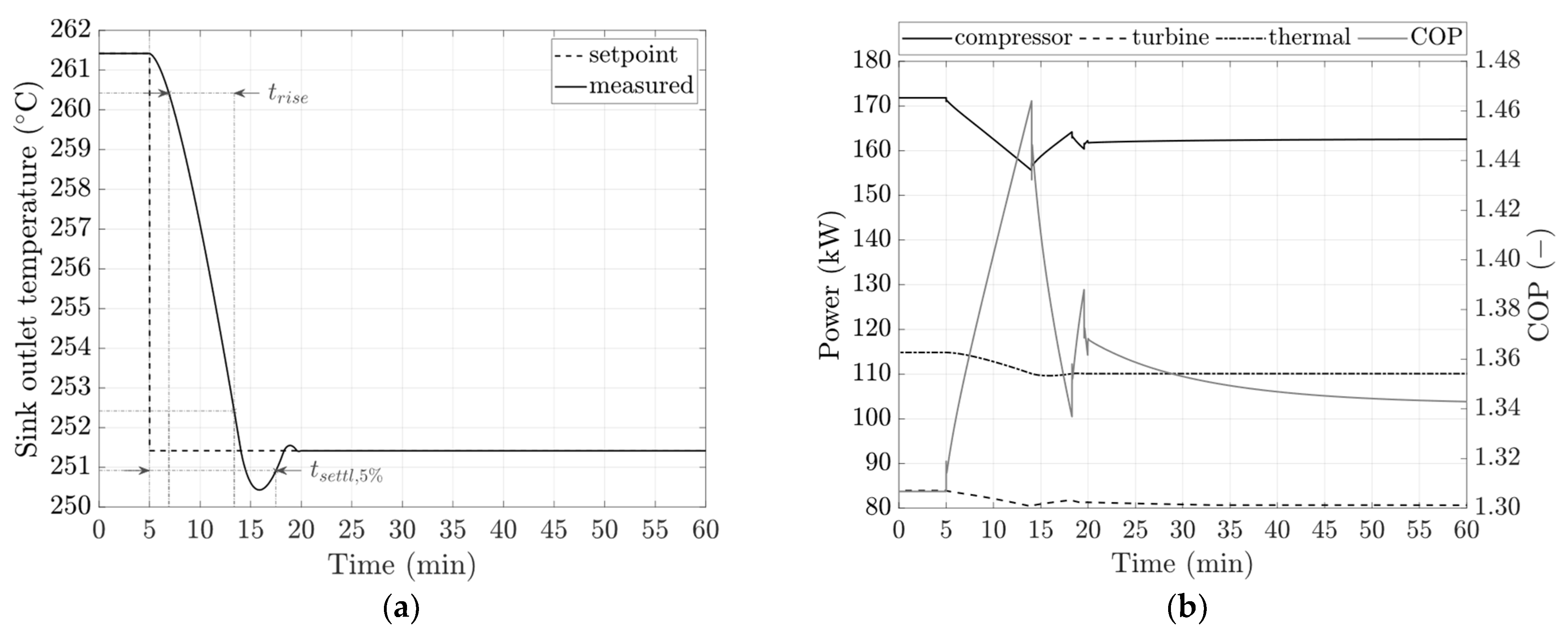
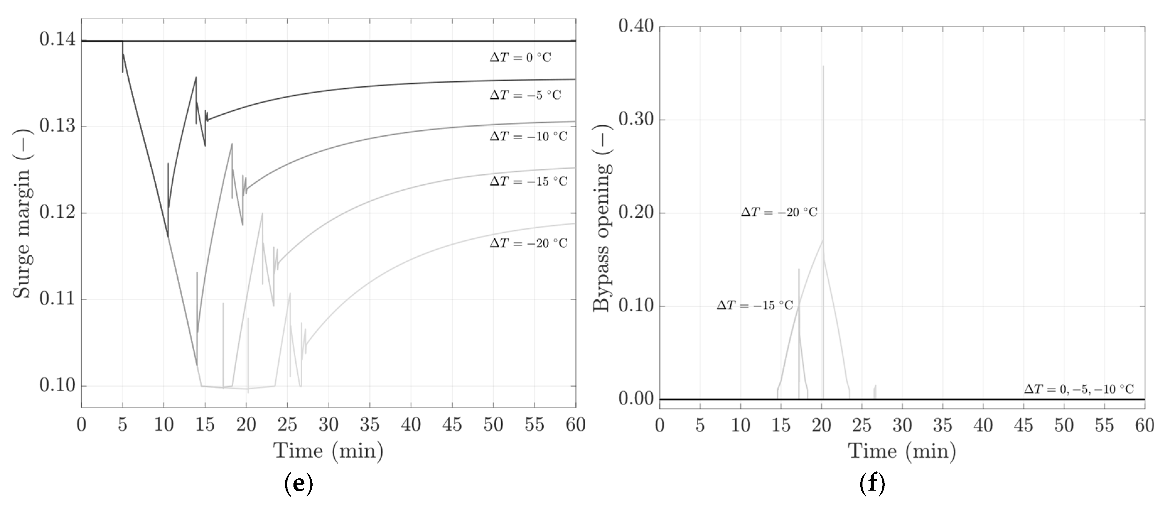
4.2. Sink Outlet Temperature Variation and Temperature/Speed Control

Figure 7 shows the heat pump response to a sudden variation of the desired temperature at the sink. At $t$ = 0 min, the system heats the sink mass flow rate from 15 °C to approximately 261.4 °C (Figure 7a). At $t$= 5 min, the temperature setpoint is reduced by −10 °C. According to Figure 7c, the temperature control reduces the compressor speed to deliver a lower and colder mass flow rate to the HTHE to accommodate setpoint variation. Since both the mass flow rate circulating in the closed loop and the compressor discharge temperature reduces, less heat transfers through the HTHE. Consequently, the temperature of the sink mass flow exiting the HTHE decreases until it reaches the new demanded value (Figure 7a).

During the transient phase, it can be observed that the sink temperature reduces according to a second-order response, with a settling time $(t_{settl}$) of 12.52 min and an undershoot of 7.82%. Furthermore, in the rise time ($t_{rise}$ = 6.47 min), the sink outlet temperature decreases linearly because of the temperature control. In particular, the regulator drives the compressor to ensure its outer temperature (${\mathrm{T}}_2$) does not vary at rates exceeding ± 2 K/min to prevent thermal stresses at the HTHE. As such rate values are reached during the regulation (Figure 7c), the relative speed and the sink temperature decrease constantly. Given that such a constraint limits the motor/compressor speed increment, it suggests that using heat exchangers capable of sustaining higher thermal stresses could reduce the rise time. In this phase, the surge margin reduces from 14% to about 10.4% due to compressor deceleration. As the surge margin never decreases below 10%, the ASC keeps the bypass closed (Figure 7d).

It can also be noted that, at $t$ = 15 min, the sink temperature oscillates around the desired value for approximately 3–4 min (Figure 7a) before stabilizing. Since this behavior primarily stems from the thermal inertia of the HTHE and pipes, it suggests that more advanced control schemes could be employed to manage the oscillations during the transient phase, thereby reducing the system’s response time. Finally, from $t$ = 20 min onwards, the motor speed is adapted because of the gradual stabilization of the temperatures in the system (Figure 7c).

On the other hand, it is worth analyzing how the performance of the heat pump evolves throughout the simulation. As detailed in Figure 7b, the COP increases from around 1.30 to 1.46 during the transient phase, eventually settling at 1.34 upon reaching the new operating conditions. This directly relates to the analyzed control strategy, which varies the compressor’s operating point (Figure 7e). In particular, because of the lower speed, the compressor operates at a higher efficiency and lower pressure ratio, thus absorbing less power. Although the power recovered by the turbine and supplied to the sink also reduces, they vary less significantly than the power demanded by the compressor. Hence, the plant operates at a higher COP.

It is also interesting to note in Figure 7 that both the supplied heat flow rate and the power recovered by the turbine evolve more regularly compared with the one absorbed by the compressor, primarily due to the thermal inertia of the piping and HTHE. Finally, Figure 7f reports the thermodynamic cycle at the beginning and at the end of the simulation. It can be observed that the temperature control leads to a reduction in the compressor outlet temperature and pressure, which also causes the turbine inlet and outlet temperature to reduce.

A sensitivity analysis was carried out to further assess the influence of requiring lower sink temperatures on the system’s performance. Results are shown in Figure 8, whilst

Table 3. System response properties for different reductions of the desired heat sink temperature.

∆T (°C)	trise (min)	tsettl,5% (min)	OV (%)
−5	3.93	8.5	14
−10	6.47	12.52	9.88
−15	8.75	15.82	7.82
−20	10.95	18.73	6.47

details the main characteristics of the sink outlet temperature responses instead.

In each simulation, the TC causes the motor speed and the sink temperature to decrease once the setpoint is varied (Figure 8a,d). Moreover, the rise and settling time increase almost linearly depends on the magnitude of setpoint variation.

On the other hand, Figure 8b reports the system’s coefficient of performance, which reaches higher values the lower the compressor rotates. As previously noted, higher values are reached during the transient phase, since the compressor rotates at speeds lower than the new steady conditions (hence higher efficiency). Moreover, Figure 8e,f report the compressor surge margin and bypass opening, respectively. Here, it can be observed that the temperature step magnitude of ∆T = {−15 °C, −20 °C} prompts the anti-surge regulator to open the turbine bypass in order to avoid compressor surge.

The outcomes of the analysis can be summarized as follows:

• Varying the compressor speed to change the sink temperature ensures a regulation time of about 8–20 min, depending on the required heat sink temperature variation;
• The system response time is limited by the maximum thermal stress that the heat exchangers can endure. The higher the allowed stress, the shorter the regulation time;
• Such a control approach causes the heat pumps to operate at higher COPs, as the net power absorbed by the system reduces more than the heat flow rate provided at the sink;
• Such a control approach can lead to compressor surge for large sink temperature variations.

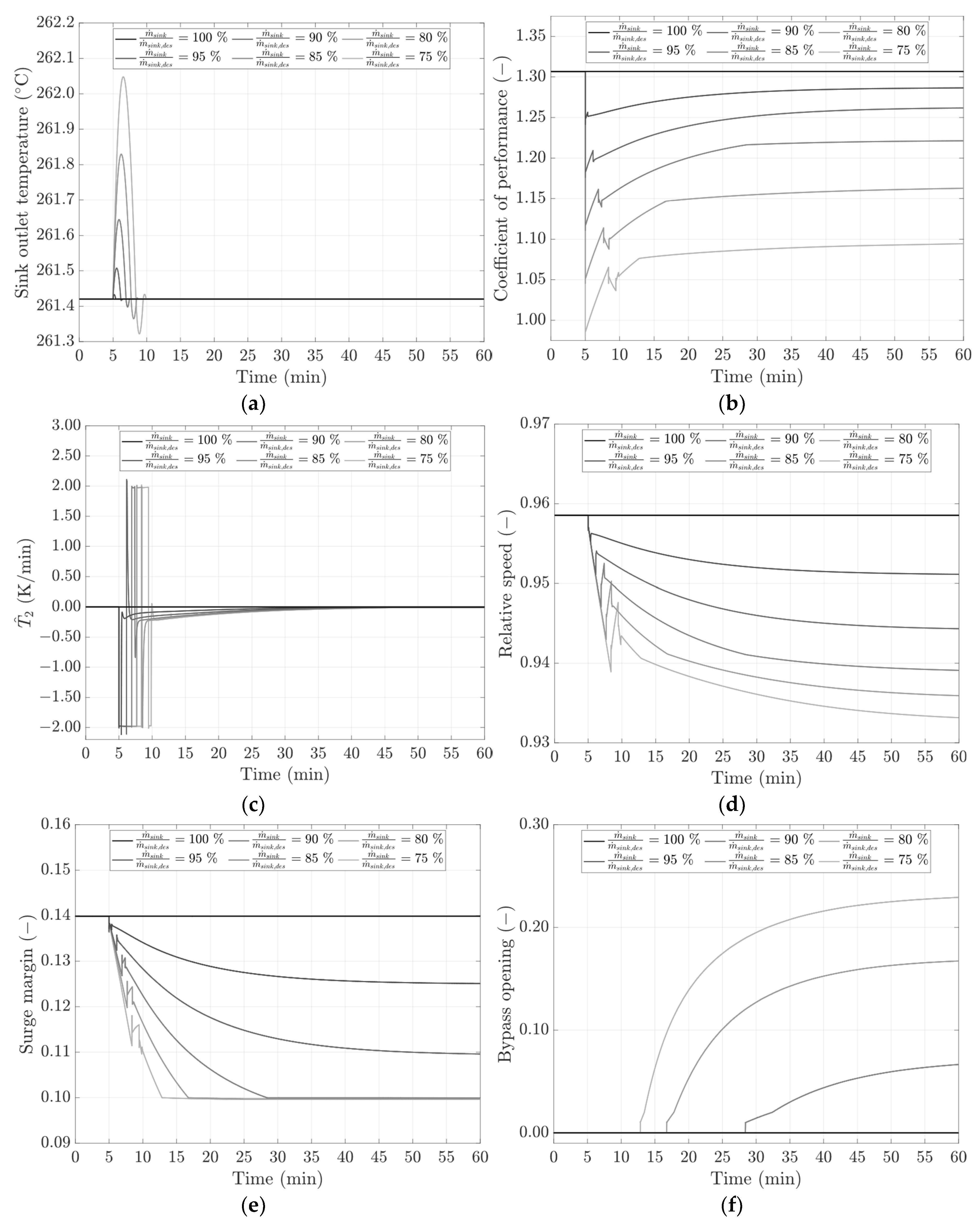
4.3. Sink Mass Flow Rate Variation and Temperature/Speed Control

Figure 9 shows the system evolution due to an abrupt variation of the sink mass flow rate while the temperature/speed control is used to maintain the sink outlet temperature constant. The goal of the simulation is to investigate how the system, regulated by varying the compressor speed, behaves in part-load conditions.

As depicted in Figure 9a, the system initially operates at nominal conditions (Table 1), and the sink mass flow rate suddenly decreases by 10% of the design value at $t$ = 5 min. As the variation occurs, the sink outlet temperature remains almost constant, mostly due to the thermal capacity of the HTHE, which absorbs the exceeding thermal power from the closed cycle, preventing significant fluctuations. In particular, the sink outlet temperature experiences only a minor increase of approximately 0.1 °C, which decays after nearly 2 min.

Since the secondary process demands reduced thermal power, the system reacts by adjusting the compressor speed to provide a lower and colder mass flow at the sink. Therefore, the compressor operating point moves towards the left part of the map at almost constant pressure ratio (Figure 9e), and the surge margin reduces from 14% to 11%, although never crossing the critical limit of 10% assumed in this work (Figure 9d).

As depicted in Figure 9c, the temperature control action is more intense as the perturbation occurs, whilst the deceleration is more gradual once the heat exchangers and piping stabilize in temperature. It can be noted in Figure 9c that the temperature rate measured at the compressor outlet saturates during the transient phase. Therefore, analogously to the previously considered scenario, higher allowable rates can improve the system response as long as the motor speed ramp limit is not exceeded.

Conversely, Figure 9b reports the system performance during the simulation. As the sink mass flow variation reduces at $t$ = 5 min, the COP suddenly decreases from 1.30 to around 1.18 due to the secondary process absorbing less thermal power. Subsequently, the heat pump COP gradually increases to approximately 1.26 because of the compressor speed regulation. It can be noted in Figure 9f that the thermodynamic cycle shrinks as the new operating conditions are met, resulting in a lower net power absorbed by the heat pump.

Also in this case, a sensitivity analysis is performed by reducing the sink mass flow rate up to 25% of the design value. Results are reported in Figure 10. As shown in Figure 10a, the higher the sink mass flow decrement, the higher the perturbation experienced by the sink outlet temperature and the longer it takes to repristinate the desired operating sink temperature.

Despite the abrupt variations, the temperature controller, combined with the thermal inertia of the system, contains the sink outlet temperature residual below ± 1 °C. In particular, for a variation of 25% of the nominal sink mass flow rate, the sink outlet temperature reaches a peak of 262.05 °C and stabilizes after $t$= 10 min.

Furthermore, larger sink mass flow variations cause the compressor to operate at lower speeds (Figure 10d), eventually leading to the operating point close to the surge line. For instance, it can be observed in Figure 10e that variations of −15%, −20%, and −25% in the sink mass flow rate cause the surge margin to approach its safety threshold, hence causing the anti-surge controller to open the turbine bypass to prevent compressor surge (Figure 10f). Concerning the system performance, the COP progressively decreases the higher the sink mass variation is (Figure 10b). In summary, the following observations can be made:

• Adjusting the compressor speed enables the heat pump to keep the heat sink temperature deviation below 1 °C in response to step changes in the sink mass flow rate. The oscillations in the sink outlet temperature are dampened within 2 to 5 min, depending on the reduction in the sink mass flow rate;
• Allowing higher thermal stress at the heat exchangers may reduce the time required to stabilize the heat sink temperature;
• Employing such a control strategy approach results in the system operating at lower COPs. Notably, higher reductions in the sink mass flow lead to decreased COPs;
• Such a control approach can lead to compressor surge in case of a significant reduction in the sink mass flow rate.

4.4. Sink Mass Flow Rate Variation through Inventory Control

Figure 11 reports the system response to a step variation of the sink mass flow rate while the inventory control regulates the sink outlet temperature at the design value. A further control loop, similar to the temperature control inner loop, is used to maintain the compressor operating speed.

As in the previously considered scenarios, the system initially operates at nominal conditions (Table 1), and the sink mass flow rate suddenly reduces by 10% of the design value at $t$ = 5 min. As shown in Figure 11a, the sink outlet temperature increases by nearly 0.6 °C to settle at the design value after around 15 min. As the secondary process demands less thermal power, the inventory control system extracts mass from the close cycle, reducing the primary mass flow (hence the thermal load supplied to the HTHE) to stabilize the sink outlet temperature (Figure 11c). Here, it can be observed that the primary mass flow experiences some fluctuations during the transient phase before stabilizing to the new operating condition.

Reducing the closed loop mass flow by means of inventory control causes the cycle pressure to decrease, as shown in Figure 11f. As the compressor speed operates at a constant speed and its inlet temperature does not vary consistently due to the LTHE, its operating point experiences only a minor perturbation, moving towards a lower pressure ratio at almost the same efficiency (Figure 11e). It can also be noted in Figure 11d that the surge margin drops as the sink mass flow rate reduction occurs and then gradually increases as air is removed from the closed cycle. Since the surge margin is always above 10%, the turbine bypass remains closed (Figure 11d).

Concerning the system performance, the COP increases from 1.30 to 1.35 after manifesting some oscillation during the transient phase. Notably, the COP increment is related to the rise in the sink and source heat exchangers’ effectiveness caused by the variation in the sink and closed cycle mass flow rates (the source mass flow rate is maintained constant). Hence, when comparing the fluid inventory control against the temperature/speed regulation, it can be observed that, for a given sink mass flow decrement, the former is more advantageous in terms of overall system performance, although characterized by a longer response time and higher peaks of the sink outlet temperature residual.

Similar to the previous scenarios, a sensitivity analysis is carried out to investigate the behavior of the system when controlled with the inventory control. Results are shown in Figure 12. It can be observed that the higher the sink mass flow reduction, the higher the sink outlet temperature residual is, which exceeds 1 °C in case of variations of −20% and −25%. Conversely, the time required from the inventory control to stabilize the sink outlet temperature remains almost the same, approximately 15 min.

The amount of fluid mass extracted from the closed cycle increases based on the sink mass flow reduction (Figure 12f), causing the primary mass flow to decrease accordingly (Figure 12e). Since mass flow circulating in the closed cycle reduces as an effect of the inventory control, the surge margin tends to reach higher values once the new operating conditions are met (Figure 12c). Moreover, as it remains above the safety threshold, the anti-surge control maintains the turbine bypass closed in each considered simulation (Figure 12d).

For what concerns the system performance, Figure 7b shows the higher sink mass flow reduction results in higher steady-state COP values. Nevertheless, fluctuations are still present during the transient phase as the results of the control action. In summary:

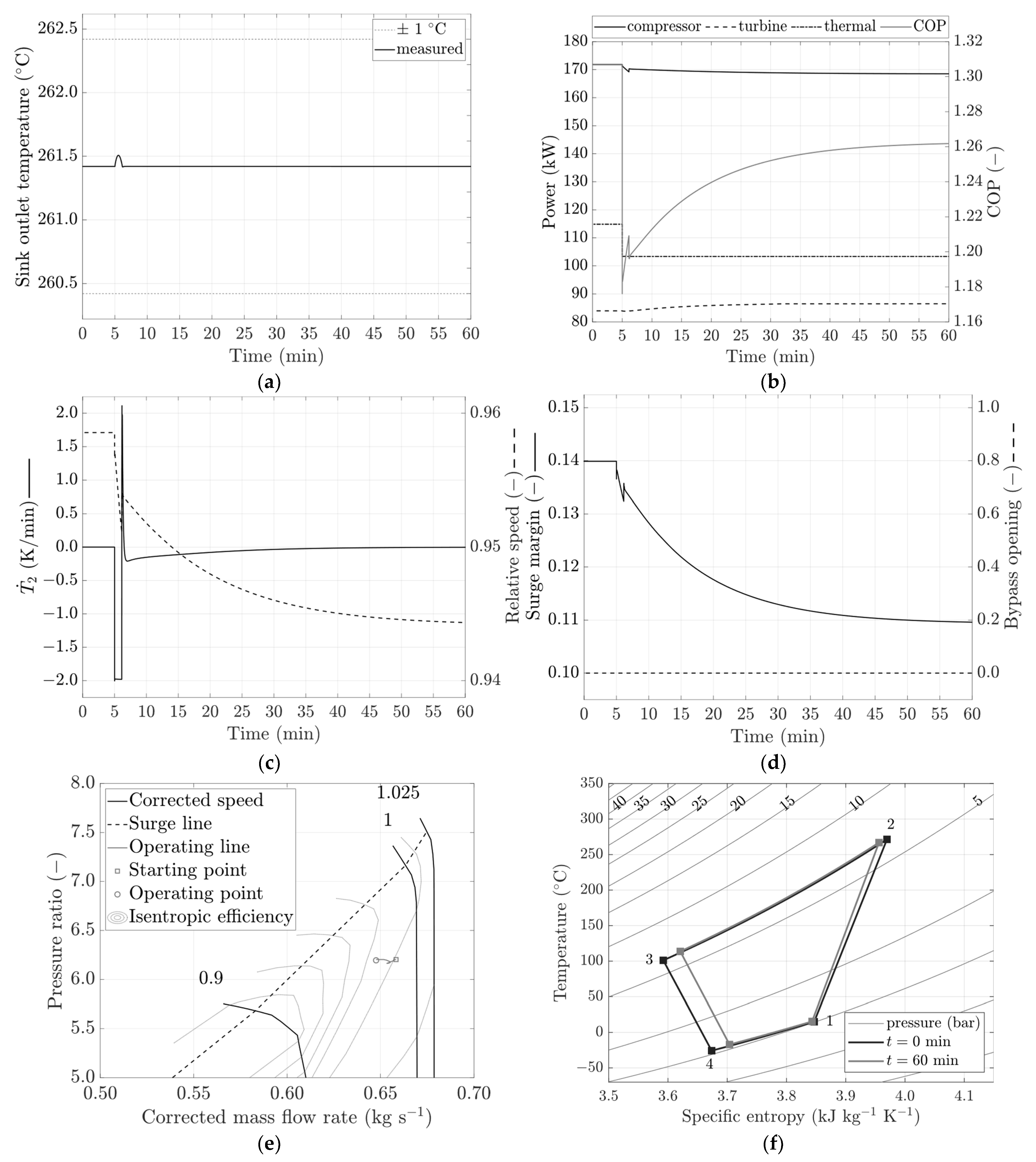
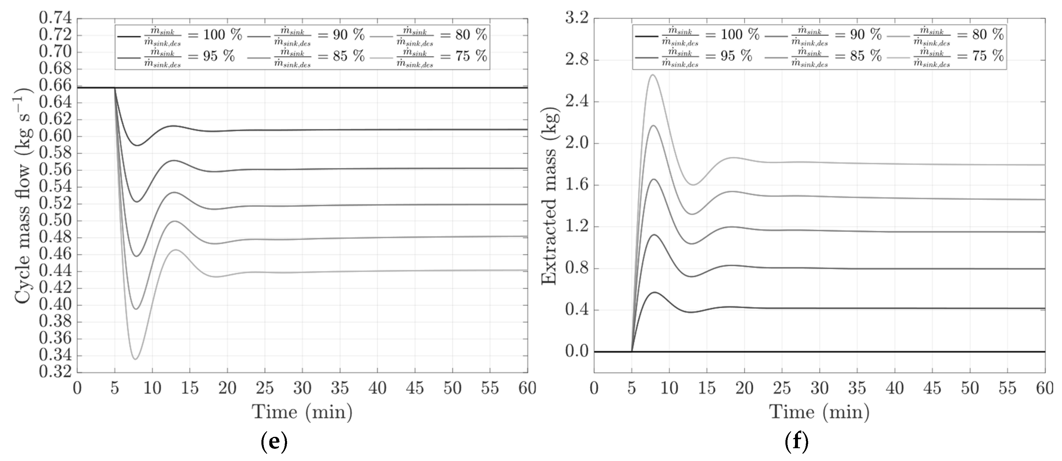
• The inventory control allows the heat pump to maintain the heat sink temperature deviation below 1.5 °C in response to step variation in the sink mass flow rate. Transient oscillations subside within 15 min, and larger variations cause higher temperature residuals during the transient phase;
• This control approach can lead to sub-ambient pressure at the compressor inlet;
• The inventory control enables the system to operate at higher COPs in new steady conditions. In particular, as the sink mass flow reduction increases, so does the COP;
• The inventory control approach does not cause compressor surge, even in scenarios involving large reductions in the sink mass flow rate.

5. Conclusions

This study investigated the transient behavior of a Brayton heat pump in the following two reference test cases: an abrupt decrease in the desired temperature at the sink and a reduction in the mass flow rate at the sink. A dynamic model of the system was built in Matlab^® R2022b, and different control strategies, namely compressor speed and fluid inventory control, were examined to adjust the system thermal load to either vary or maintain the sink outlet temperature at the desired value. Findings are summarized below.

• When varying the compressor speed to regulate the heat sink temperature, the system reduces the sink temperature to new desired values according to a second-order system response, and the larger the desired sink outlet temperature reduction, the longer the response time. Additionally, the rate at which the sink outlet temperature increases is bounded by the maximum allowed temperature rate at the compressor outlet;
• When varying the compressor speed to maintain the heat sink temperature in response to a 10% reduction in the sink mass flow, the sink outlet temperature experiences only a minor oscillation, which dampens after about 5 min. The system COP reduces once the new steady-state conditions are met. Larger sink mass flow reductions cause higher heat sink temperature residuals during the transient phase (although always below ± 1 °C) and progressively lower COPs;
• When using the inventory control to maintain the sink outlet in response to a 10% reduction in the sink mass flow, the sink outlet temperature deviates by about 0.6 °C from the nominal value during the transient phase and stabilizes after nearly 15 min. The system COP increases by about 0.05 compared with nominal operating conditions. Larger sink mass flow rate reductions lead to higher heat sink temperature residuals during the transient phase (always below 1.5 °C) and progressively higher COPs;
• When comparing the considered control strategies to maintain the desired heat sink temperature in response to a sudden reduction in the sink mass flow, varying the compressor speed allows for lower sink outlet temperature perturbations (e.g., 0.1 °C vs. 0.6 °C) and faster response times (e.g., 5 min vs. 15 min). On the other hand, the fluid inventory control enables the system to operate at higher COPs (e.g., 1.35 vs. 1.26) when new operating conditions are met. Moreover, unlike the speed regulation approach, the inventory control approach ensures large surge margins, reducing the risk of compressor surge.

As a final remark, this study suggests that a hybrid approach combining speed and inventory control would be advantageous as it could lead to both lower temperature variation and high COP during transient phases. This control approach will be the subject of future research.

References

- IEA. Heating; IEA: Paris, France, 2022; Available online: https://www.iea.org/reports/heating (accessed on 10 January 2024).
- IEA. The Future of Heat Pumps; IEA: Paris, France, 2022; Available online: https://www.iea.org/reports/the-future-of-heat-pumps (accessed on 10 January 2024).
- Wolf, S.; Blesl, M. Model-Based Quantification of the Contribution of Industrial Heat Pumps to the European Climate Change Mitigation Strategy. In ECEEE Industrial Summer Study Proceedings; ECEEE: Berlin, Germany, 2016; pp. 477–487. [Google Scholar]
- Gai, L.; Varbanov, P.S.; Walmsley, T.G.; Klemeš, J.J. Critical Analysis of Process Integration Options for Joule-Cycle and Conventional Heat Pumps. Energies 2020, 13, 635. [Google Scholar] [CrossRef]
- Arpagaus, C.; Bless, F.; Uhlmann, M.; Schiffmann, J.; Bertsch, S.S. High Temperature Heat Pumps: Market Overview, State of the Art, Research Status, Refrigerants, and Application Potentials. Energy 2018, 152, 985–1010. [Google Scholar] [CrossRef]
- Naegler, T.; Simon, S.; Klein, M.; Gils, H.C. Quantification of the European Industrial Heat Demand by Branch and Temperature Level: Quantification of European Industrial Heat Demand. Int. J. Energy Res. 2015, 39, 2019–2030. [Google Scholar] [CrossRef]
- Rehfeldt, M.; Fleiter, T.; Toro, F. A Bottom-up Estimation of the Heating and Cooling Demand in European Industry. Energy Effic. 2018, 11, 1057–1082. [Google Scholar] [CrossRef]
- Bless, F.; Arpagaus, C.; Bertsch, S.S.; Schiffmann, J. Theoretical Analysis of Steam Generation Methods—Energy, CO2 Emission, and Cost Analysis. Energy 2017, 129, 114–121. [Google Scholar] [CrossRef]
- Jesper, M.; Schlosser, F.; Pag, F.; Walmsley, T.G.; Schmitt, B.; Vajen, K. Large-Scale Heat Pumps: Uptake and Performance Modelling of Market-Available Devices. Renew. Sustain. Energy Rev. 2021, 137, 110646. [Google Scholar] [CrossRef]
- Zühlsdorf, B.; Bühler, F.; Bantle, M.; Elmegaard, B. Analysis of Technologies and Potentials for Heat Pump-Based Process Heat Supply above 150 °C. Energy Convers. Manag. X 2019, 2, 100011. [Google Scholar] [CrossRef]
- Smith, N.R.; Tom, B.; Rimpel, A.; Just, J.; Marshall, M.; Khawly, G.; Revak, T.; Hoopes, K. The Design of a Small-Scale Pumped Heat Energy Storage System for the Demonstration of Controls and Operability. In Volume 4: Cycle Innovations: Energy Storage; Proceedings of the ASME Turbo Expo 2022: Turbomachinery Technical Conference and Exposition, Rotterdam, The Netherlands, 13–17 June 2022; American Society of Mechanical Engineers: New York, NY, USA, 2022; Volume 4. [Google Scholar] [CrossRef]
- Oehler, J.; Tran, A.P.; Stathopoulos, P. Simulation of a Safe Start-Up Maneuver for a Brayton Heat Pump. In Volume 4: Cycle Innovations: Energy Storage; Proceedings of the ASME Turbo Expo 2022: Turbomachinery Technical Conference and Exposition, Rotterdam, The Netherlands, 13–17 June 2022; American Society of Mechanical Engineers: New York, NY, USA, 2022; Volume 4, p. V004T06A003. [Google Scholar] [CrossRef]
- Ferrari, L.; Pettinari, M.; Frate, G.F.; Tran, A.P.; Oehler, J.; Stathopoulos, P. Transient Analysis and Control of a Brayton Heat Pump During Start-Up. In Proceedings of the 36th International Conference on Efficiency, Cost, Optimization, Simulation and Environmental Impact of Energy Systems (ECOS 2023), Las Palmas De Gran Canaria, Spain, 25–30 June 2023; pp. 839–850. [Google Scholar] [CrossRef]
- Pettinari, M.; Frate, G.F.; Kyprianidis, K.; Ferrari, L. Dynamic Modelling and Part-Load Behavior of a Brayton Heat Pump. In Proceedings of the 64th International Conference of Scandinavian Simulation Society, SIMS 2023, Västerås, Sweden, 25–28 September 2023; pp. 254–261. [Google Scholar] [CrossRef]
- The MathWorks Inc. MATLAB Version: 9.13.0 (R2022b). 2022. Available online: https://www.mathworks.com (accessed on 10 January 2024).
- Lemmon, E.W.; Bell, I.H.; Huber, M.L.; McLinden, M.O. NIST Standard Reference Database 23: Reference Fluid Thermodynamic and Transport Properties-REFPROP, Version 10.0; National Institute of Standards and Technology: Gaithersburg, MD, USA, 2018.
- The MathWorks Inc. Simscape Fluids Reference. Available online: https://it.mathworks.com/help/pdf_doc/hydro/hydro_ref.pdf (accessed on 10 January 2024).
- Holman, J.P. Heat Transfer, 9th ed.; McGraw-Hill: New York, NY, USA, 2002; ISBN 978-0-07-352936-3. [Google Scholar]
- White, F.M. Fluid Mechanics, 7th ed.; McGraw-Hill Series in Mechanical Engineering; McGraw-Hill: New York, NY, USA, 2011; ISBN 978-0-07-352934-9. [Google Scholar]